The effects of juniper treatments on grazing productivity

An Integrated Landscape Assessment Project(ILAP) Case Study of Economic Costs and Benefits

Treg Christopher & Megan Creutzburg

NatureServe BWB Conference April 24, 2012

Photo: Treg Christopher

Juniper Encroachment

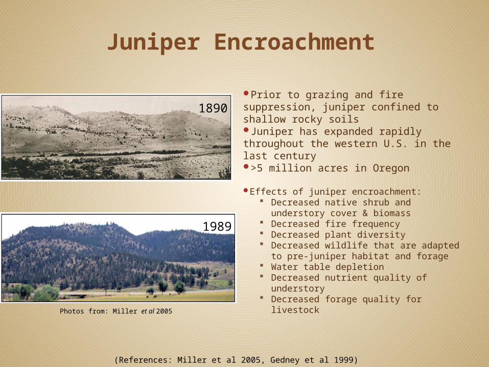
1890

1989

Photos from: Miller et al 2005

Prior to grazing and fire suppression, juniper confined to shallow rocky soilsJuniper has expanded rapidly throughout the western U.S. in the last century>5 million acres in Oregon

Effects of juniper encroachment: Decreased native shrub and

understory cover & biomass Decreased fire frequency Decreased plant diversity Decreased wildlife that are adapted to

pre-juniper habitat and forage Water table depletion Decreased nutrient quality of

understory Decreased forage quality for livestock

(References: Miller et al 2005, Gedney et al 1999)

Grazing on the Landscape

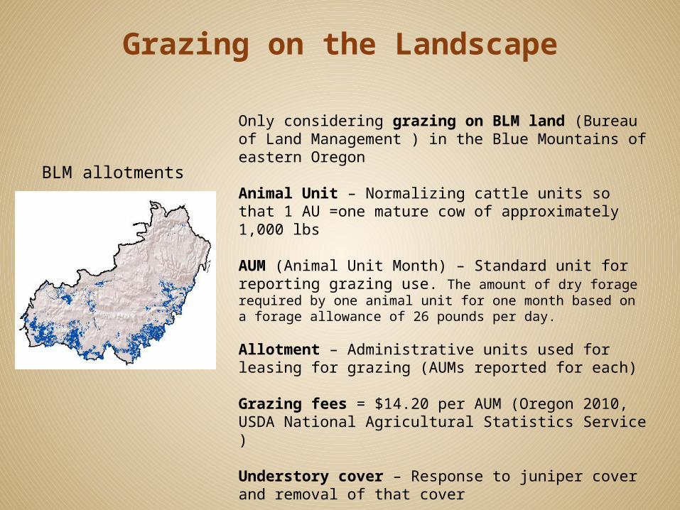
Only considering grazing on BLM land (Bureau of Land Management ) in the Blue Mountains of eastern Oregon

Animal Unit – Normalizing cattle units so that 1 AU =one mature cow of approximately 1,000 lbs

AUM (Animal Unit Month) – Standard unit for reporting grazing use. The amount of dry forage required by one animal unit for one month based on a forage allowance of 26 pounds per day. Allotment – Administrative units used for leasing for grazing (AUMs reported for each)

Grazing fees = $14.20 per AUM (Oregon 2010, USDA National Agricultural Statistics Service )

Understory cover – Response to juniper cover and removal of that cover

Normalized Biomass – understory cover so that max grazing capacity (in AUMs) =1 and biomass in heavy juniper < 1

BLM allotments

Ecosystem Services & Valuation

Damages caused by juniper encroachment: Direct use/ provisioning services (loss of grazing capacity) Indirect use / supporting or regulating services (soil stabilization

and soil water storage) Non-use / cultural services (loss of rare and endangered species,

or aesthetics of an open landscape)

This study only considers one type of direct use values, loss of grazing capacity and associated economic value, loss of grazing fees

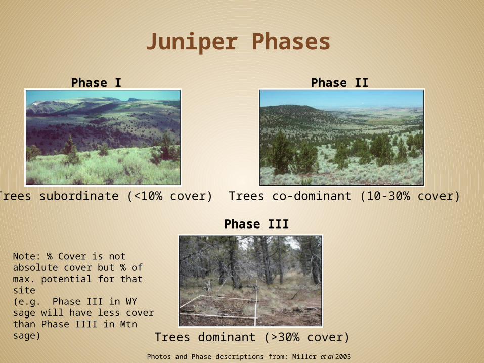
Juniper Phases

Phase I Phase II

Phase III

Photos and Phase descriptions from: Miller et al 2005

Trees co-dominant (10-30% cover)

Trees dominant (>30% cover)

Trees subordinate (<10% cover)

Note: % Cover is not absolute cover but % of max. potential for that site(e.g. Phase III in WY sage will have less cover than Phase IIII in Mtn sage)

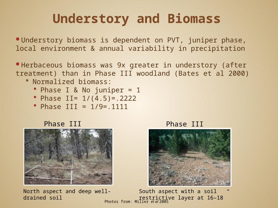
Understory and Biomass

Phase IIIPhase III

Photos from: Miller et al 2005

Understory biomass is dependent on PVT, juniper phase, local environment & annual variability in precipitation

Herbaceous biomass was 9x greater in understory (after treatment) than in Phase III woodland (Bates et al 2000)

Normalized biomass: Phase I & No juniper = 1 Phase II= 1/(4.5)=.2222 Phase III = 1/9=.1111

South aspect with a soil restrictive layer at 16–18”

North aspect and deep well-drained soil

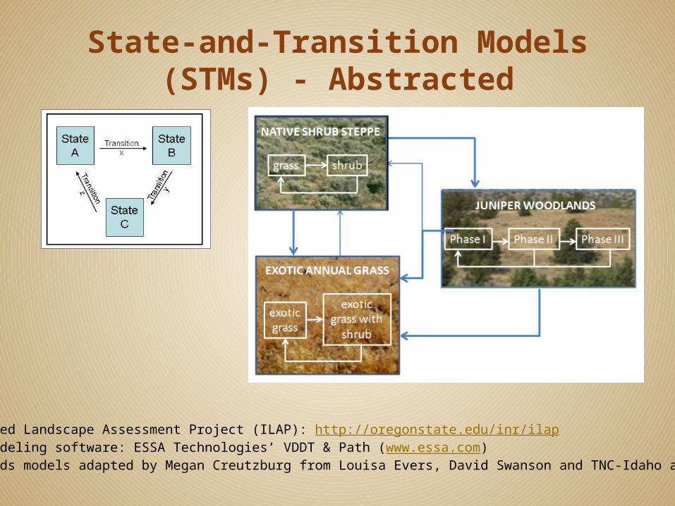
State-and-Transition Models (STMs) - Abstracted

Integrated Landscape Assessment Project (ILAP): http://oregonstate.edu/inr/ilap ILAP modeling software: ESSA Technologies’ VDDT & Path (www.essa.com)Arid lands models adapted by Megan Creutzburg from Louisa Evers, David Swanson and TNC-Idaho and Nevada

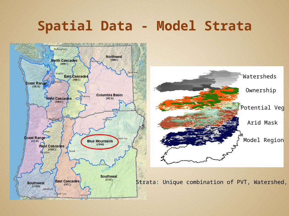
Spatial Data - Model Strata

Strata: Unique combination of PVT, Watershed, Owner

Watersheds

Ownership

Potential Veg

Arid Mask

Model Region

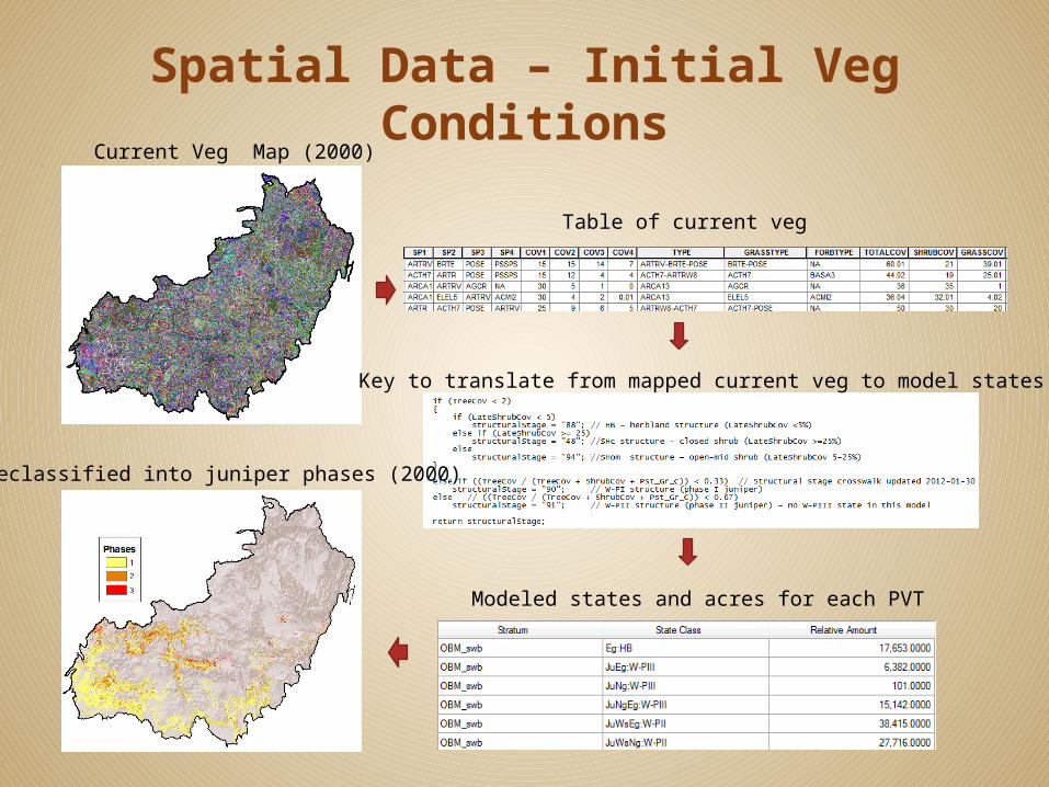
Spatial Data – Initial Veg Conditions

Current Veg Map (2000)

Reclassified into juniper phases (2000)

Table of current veg

Key to translate from mapped current veg to model states

Modeled states and acres for each PVT

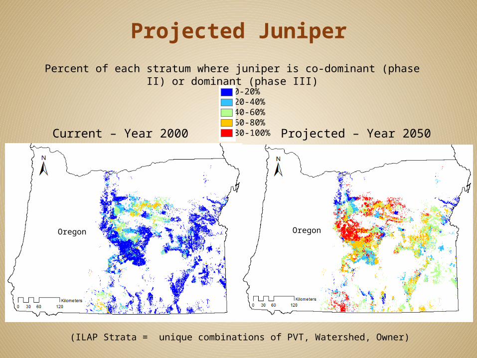
Projected Juniper

Oregon Oregon

Projected – Year 2050Current – Year 2000

Percent of each stratum where juniper is co-dominant (phase II) or dominant (phase III)

0-20%20-40%40-60%60-80%80-100%

(ILAP Strata = unique combinations of PVT, Watershed, Owner)

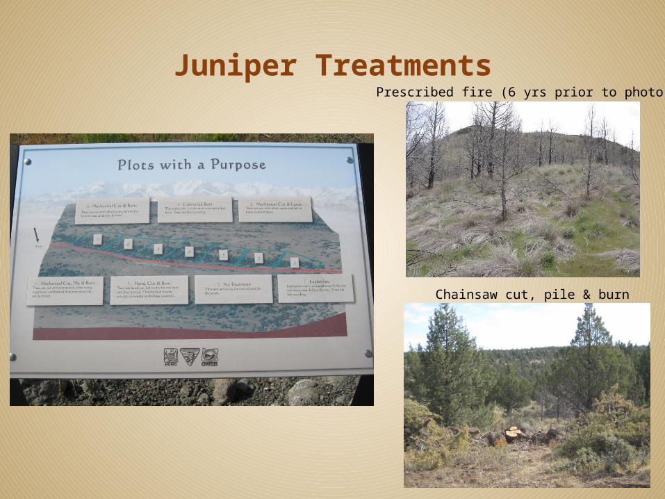
Juniper TreatmentsPrescribed fire (6 yrs prior to photo)

Chainsaw cut, pile & burn

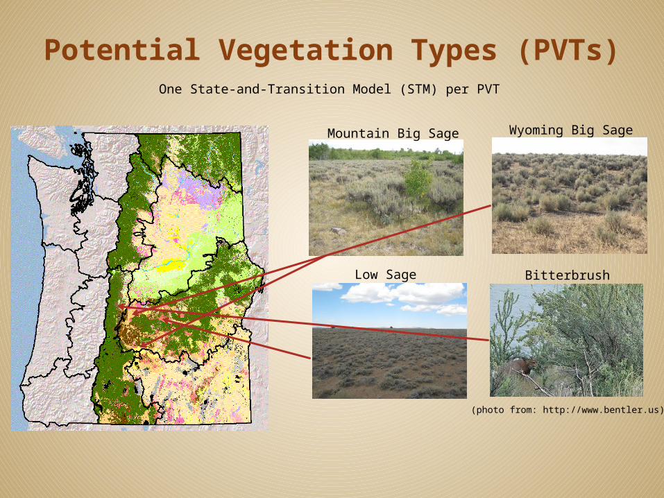
Potential Vegetation Types (PVTs)

Low Sage

Mountain Big Sage Wyoming Big Sage

Bitterbrush

(photo from: http://www.bentler.us)

One State-and-Transition Model (STM) per PVT

AUM by PVT by Phases

Total AUMs in study region = 227,838

Total AUMs in 4 PVTs= 155,342

PVT Low sageMountain big sageBitterbrushWyoming big sage

Proportion of 4 PVTs in allotment area = 68%

PVT Code PVT Name Pct AUMOBM_slw Low sage 0.17 26,698

OBM_smbMountain big sage 0.35 54,101

OBM_spt Bitterbrush 0.08 11,756

OBM_swbWyoming big sage 0.40 62,786

Proportion of PVT in each phase

Normalized biomass in each phase

PVT Code Phase AUMperAcre

OBM_swb JunPhase1 0.17

OBM_swb JunPhase2 0.03

OBM_swb JunPhase3 0.02

OBM_swb NoJun 0.17

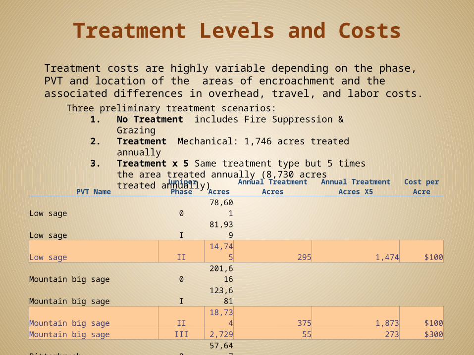
Treatment Levels and Costs

PVT Name Juniper Phase Acres Annual Treatment Acres Annual Treatment Acres X5 Cost per AcreLow sage 0 78,601Low sage I 81,939Low sage II 14,745 295 1,474 $100Mountain big sage 0 201,616Mountain big sage I 123,681Mountain big sage II 18,734 375 1,873 $100Mountain big sage III 2,729 55 273 $300Bitterbrush 0 57,647Bitterbrush I 12,704Bitterbrush II 4,877 98 488 $100Bitterbrush III 612Wyoming big sage 0 213,131Wyoming big sage I 151,442Wyoming big sage II 41,417 828 4,142 $100Wyoming big sage III 4,809 96 481 $300

Three preliminary treatment scenarios:1. No Treatment includes Fire Suppression & Grazing2. Treatment Mechanical: 1,746 acres treated annually3. Treatment x 5 Same treatment type but 5 times the

area treated annually (8,730 acres treated annually)

Treatment costs are highly variable depending on the phase, PVT and location of the areas of encroachment and the associated differences in overhead, travel, and labor costs.

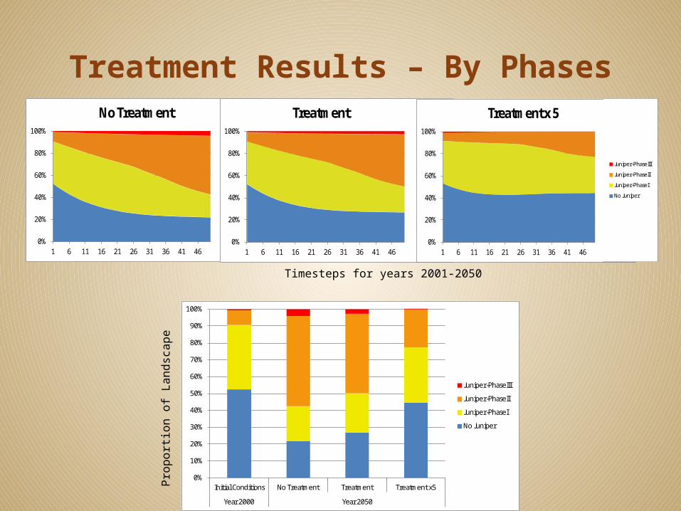
Treatment Results – By Phases

0%

10%

20%

30%

40%

50%

60%

70%

80%

90%

100%

Initial Conditions No Treatment Treatment Treatment x5

Year 2000 Year 2050

Juniper-PhaseIII

Juniper-PhaseII

Juniper-PhaseI

No Juniper

Pro

port

ion o

f La

ndsc

ape

0%

20%

40%

60%

80%

100%

1 6 11 16 21 26 31 36 41 46

No Treatment

Phase3

Phase2

Phase1

NoJun

0%

20%

40%

60%

80%

100%

1 6 11 16 21 26 31 36 41 46

Treatment

Phase3

Phase2

Phase1

NoJun

0%

20%

40%

60%

80%

100%

1 6 11 16 21 26 31 36 41 46

Treatment x 5

Phase3

Phase2

Phase1

NoJun

Timesteps for years 2001-2050

0%

10%

20%

30%

40%

50%

60%

70%

80%

90%

100%

Initial Conditions No Treatment Treatment Treatment x5

Year 2000 Year 2050

Juniper-PhaseIII

Juniper-PhaseII

Juniper-PhaseI

No Juniper

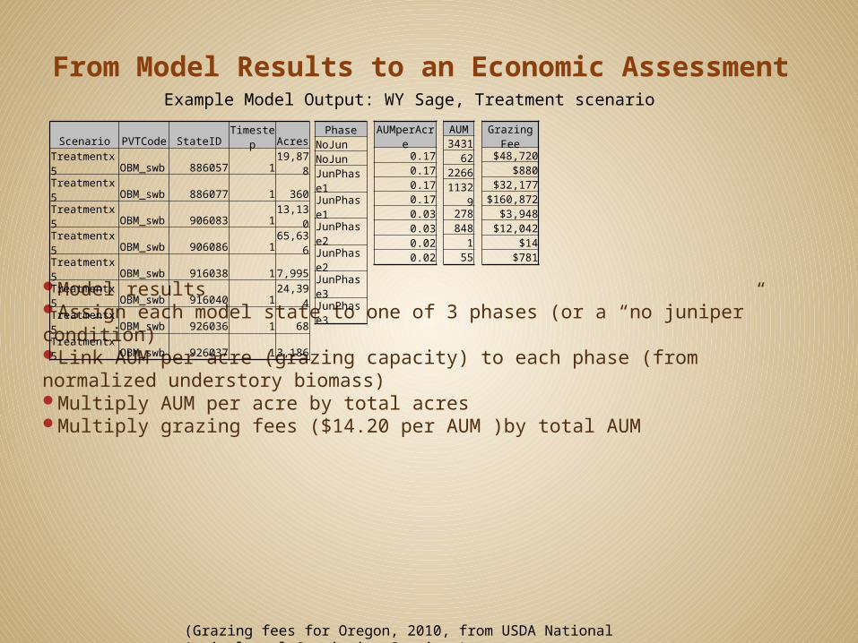
From Model Results to an Economic Assessment

Model results Assign each model state to one of 3 phases (or a “no juniper” condition)Link AUM per acre (grazing capacity) to each phase (from normalized understory biomass)Multiply AUM per acre by total acres Multiply grazing fees ($14.20 per AUM )by total AUM

Example Model Output: WY Sage, Treatment scenario

Grazing Fee$48,720

$880$32,177

$160,872$3,948

$12,042$14

$781

(Grazing fees for Oregon, 2010, from USDA National Agricultural Statistics Service )

Scenario PVTCode StateID Timestep AcresTreatmentx5 OBM_swb 886057 1 19,878Treatmentx5 OBM_swb 886077 1 360Treatmentx5 OBM_swb 906083 1 13,130Treatmentx5 OBM_swb 906086 1 65,636Treatmentx5 OBM_swb 916038 1 7,995Treatmentx5 OBM_swb 916040 1 24,394Treatmentx5 OBM_swb 926036 1 68Treatmentx5 OBM_swb 926037 1 3,186

AUMperAcre0.170.170.170.170.030.030.020.02

PhaseNoJunNoJunJunPhase1JunPhase1JunPhase2JunPhase2JunPhase3JunPhase3

AUM3431

622266

11329278848

155

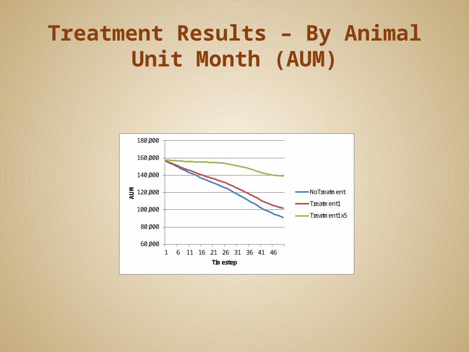
Treatment Results – By Animal Unit Month (AUM)

60,000

80,000

100,000

120,000

140,000

160,000

180,000

1 6 11 16 21 26 31 36 41 46

AU

M

Timestep

NoTreatment

Treatment1

Treatment1x5

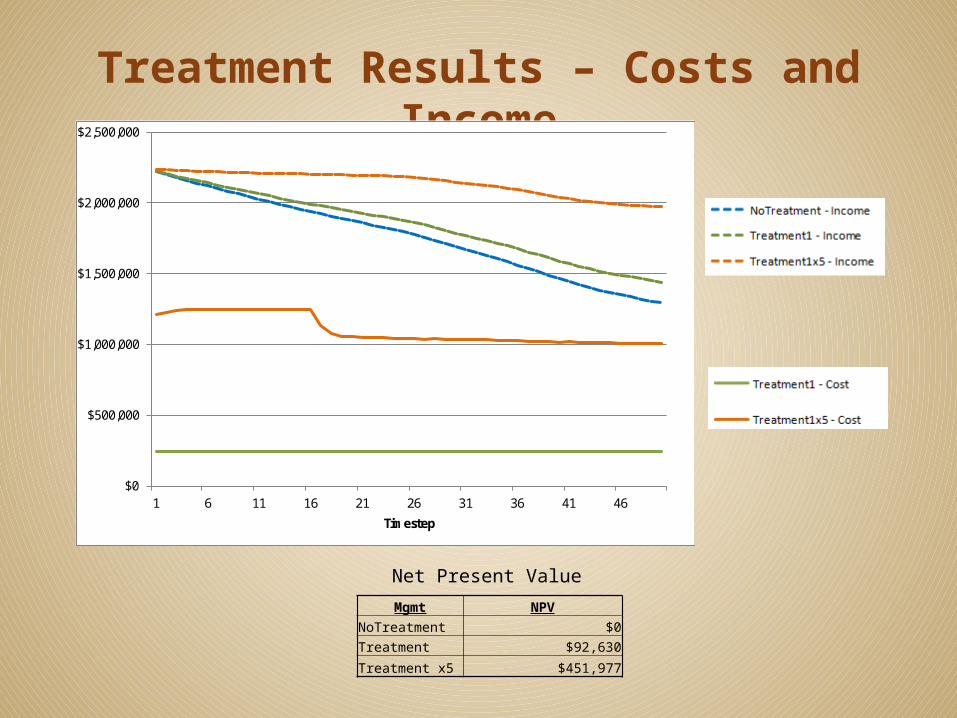
Treatment Results – Costs and Income

$0

$500,000

$1,000,000

$1,500,000

$2,000,000

$2,500,000

1 6 11 16 21 26 31 36 41 46

Timestep

NoTreatment - Cost

NoTreatment - Income

Treatment1 - Cost

Treatment1 - Income

Treatment1x5 - Cost

Treatment1x5 - Income

Mgmt NPV

NoTreatment $0

Treatment $92,630

Treatment x5 $451,977

Net Present Value

Conclusions

2 treatment levels are not sufficient to return to pre-1900 conditions

Treatment x5 has removed phase III from the landscape and reduced phase II by @ 50%

Grazing capacity (as AUMs) is reduced in all scenarios Treatment x 5 (8,730 acres treated annually) is gets much closer to maintaining

capacity

Cost : benefit results (discounted to 2010) show that treatment x 5 provides the best economic return on investment

Only one type of direct use/ provisioning service and value considered: grazing capacity & grazing fees.

Limitations - Improvements

Relationship between juniper removal and understory response by PVT and by Phases

Modeling lag in response between treatments and recovery (2-7 yrs). No lag = overestimate of benefits.

Differences in grazing capacity between PVTs (AUM is only reported by allotments)

States in Phase I and No Juniper are assumed to providing maximum capacity (ignoring degraded conditions and exotic grass invasion). This overestimates the benefits of treatments.

Better treatment cost estimates and for different treatment types Treatment costs are the same across PVTs and regardless of location (e.g.

travel cost ignored) USGS Land Treatment Digital Library (http://greatbasin.wr.usgs.gov/ltdl/) Alternative treatments (and associated costs) and annual amount of area to be

treated can be run and compared through the Path software’s Treatment Analyzer

ILAP InformationILAP website: http://oregonstate.edu/inr/ilap

FTP site for data download and documentation: ftp://131.252.97.79/ILAP/Index.html

Institute for Natural Resources’ Western Landscapes Explorer (Web-based mapping of change in states and indicators....coming soon)

ILAP modelers:Treg Christopher (treg.christopher@oregonstate.edu)Megan Creutzberg (megan.creutzberg@oregonstate.edu)Emilie Henderson (emilie.henderson@oregonstate.edu)Therese Burcsu (theresa.burcsu@oregonstate.edu )

Gedney, D.R., Azuma, D.L., Bolsinger, C.L., McKay, N., 1999. Western juniper in eastern Oregon. U.S. Forest Service General Technical Report. NW-GTR-464.Hanna, D., Korb, N., Bauer, B., Martin, B., Frid, L., Bryan, K., Holzer, B., 2011. Evaluating the Costs and Benefits of Alternative Weed Management Strategies for Three Montana Landscapes. The Nature Conservancy of Montana, Helena, MT, p. 138.Miller, R.F., Bates, J., Svejcar, A., Pierson, F., Eddleman, L., 2005. Biology, ecology, and management of western juniper (Juniperus occidentalis). Oregon State University, Agricultural Experiment Station, Corvallis, OR, p. 77.Miller, R.F., Svejcar, T.J., Rose, J.A., 2000. Impacts of Western Juniper on Plant Community Composition and Structure. Journal of Range Management 53, 574-585.Provencher, L., Forbis, T.A., Frid, L., Medlynd, G., 2007. Comparing alternative management strategies of fire, grazing, and weed control using spatial modeling. Ecological Modeling 209, 249-263.

References

End of Presentation Materials

In the second year post-cutting total understory biomass and N uptake were nearly 9 times greater in cut versus woodland treat-ments. Perennial plant basal cover was 3 times greater and plant diversity was 1.6 times greater in the cut versus woodland treat-ments. (Bates 2000)

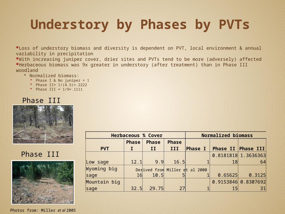
Understory by Phases by PVTs

Phase III

Phase III

Photos from: Miller et al 2005

Loss of understory biomass and diversity is dependent on PVT, local environment & annual variability in precipitationWith increasing juniper cover, drier sites and PVTs tend to be more (adversely) affectedHerbaceous biomass was 9x greater in understory (after treatment) than in Phase III woodland

Normalized biomass: Phase I & No juniper = 1 Phase II= 1/(4.5)=.2222 Phase III = 1/9=.1111

Herbaceous % Cover Normalized biomassPVT Phase I Phase II Phase III Phase I Phase II Phase III

Low sage 12.1 9.9 16.5 1 0.818181818 1.363636364Wyoming big sage 16 10.5 5 1 0.65625 0.3125Mountain big sage 32.5 29.75 27 1 0.915384615 0.830769231

Derived from Miller et al 2000

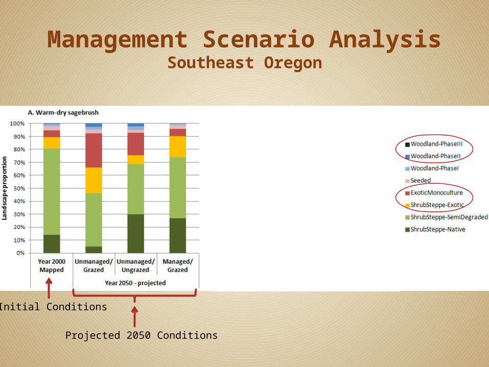
Management Scenario AnalysisSoutheast Oregon

Initial Conditions

Projected 2050 Conditions

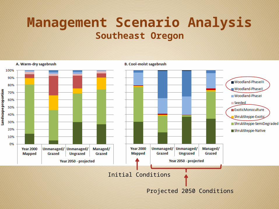
Management Scenario AnalysisSoutheast Oregon

Initial Conditions

Projected 2050 Conditions

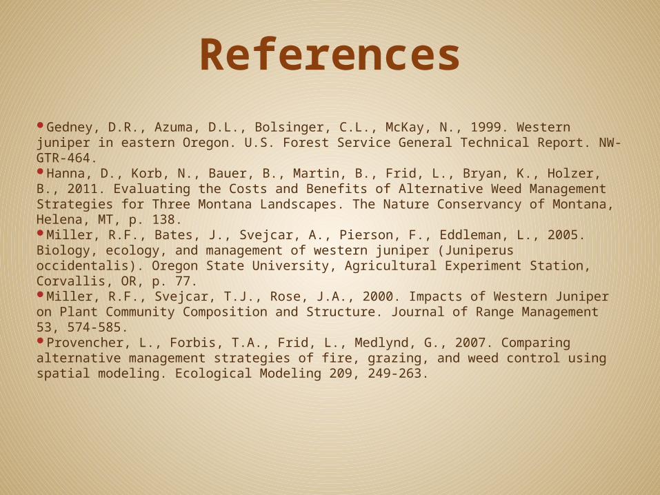
ReferencesGedney, D.R., Azuma, D.L., Bolsinger, C.L., McKay, N., 1999. Western juniper in eastern Oregon. U.S. Forest Service General Technical Report. NW-GTR-464.Hanna, D., Korb, N., Bauer, B., Martin, B., Frid, L., Bryan, K., Holzer, B., 2011. Evaluating the Costs and Benefits of Alternative Weed Management Strategies for Three Montana Landscapes. The Nature Conservancy of Montana, Helena, MT, p. 138.Miller, R.F., Bates, J., Svejcar, A., Pierson, F., Eddleman, L., 2005. Biology, ecology, and management of western juniper (Juniperus occidentalis). Oregon State University, Agricultural Experiment Station, Corvallis, OR, p. 77.Miller, R.F., Svejcar, T.J., Rose, J.A., 2000. Impacts of Western Juniper on Plant Community Composition and Structure. Journal of Range Management 53, 574-585.Provencher, L., Forbis, T.A., Frid, L., Medlynd, G., 2007. Comparing alternative management strategies of fire, grazing, and weed control using spatial modeling. Ecological Modeling 209, 249-263.

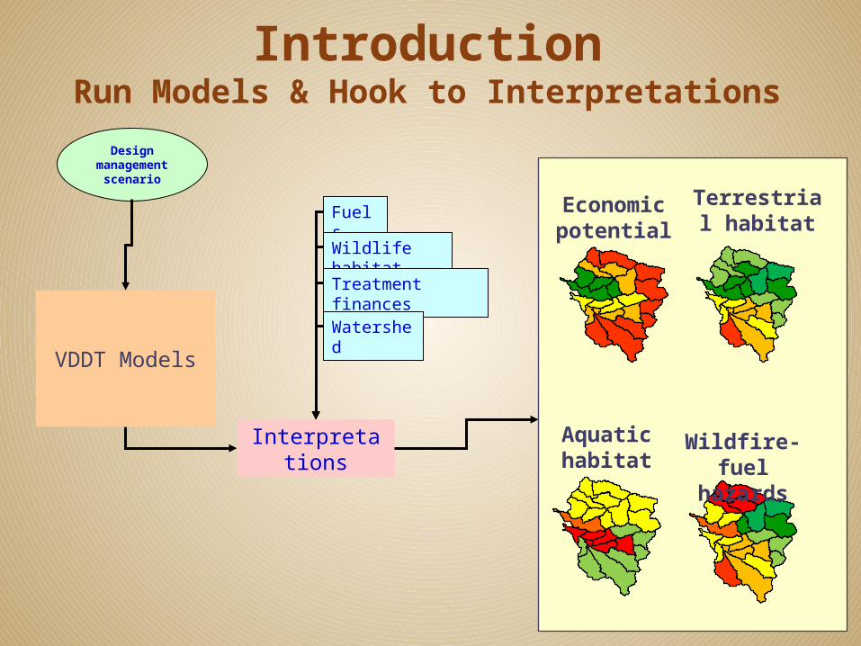
IntroductionRun Models & Hook to Interpretations

Fuels

Wildlife habitatTreatment finances

Interpretations

Watershed

Design management

scenario

VDDT Models

Wildfire-fuel

hazards

Terrestrial habitat

Aquatic habitat

Economic potential

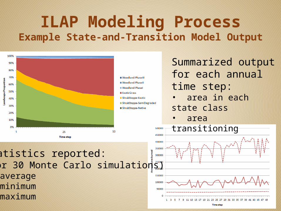
ILAP Modeling ProcessExample State-and-Transition Model Output

Summarized output for each annual time step:• area in each state class• area transitioning

Statistics reported:(for 30 Monte Carlo simulations)• average• minimum• maximum

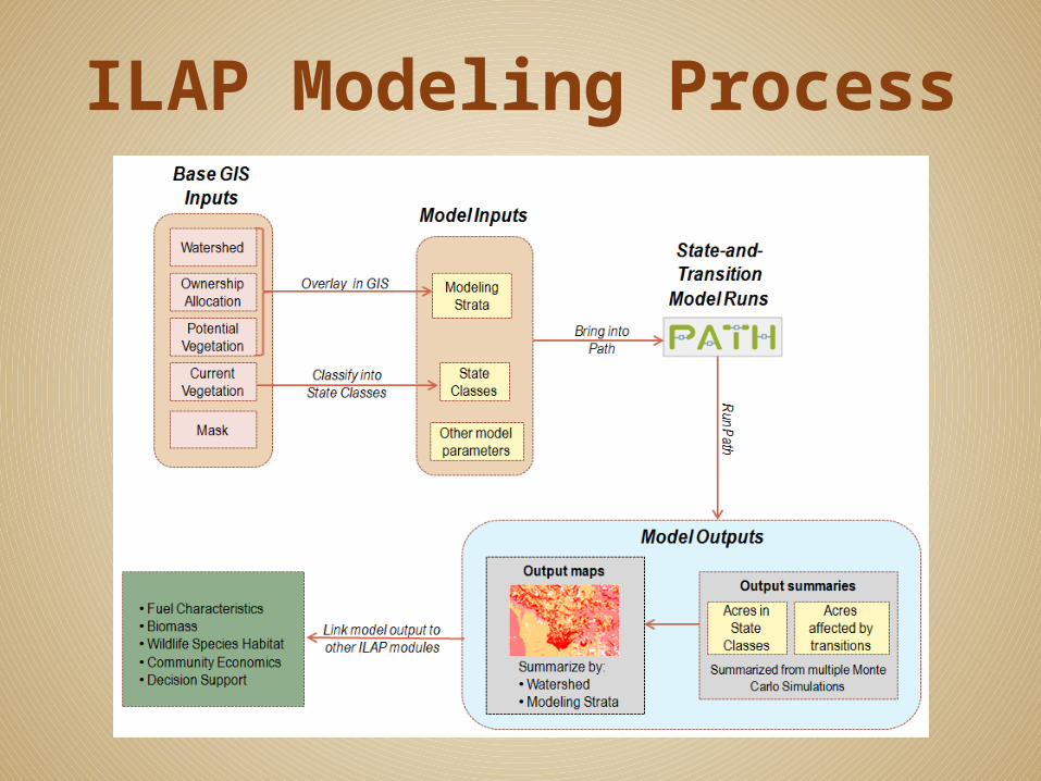
ILAP Modeling Process