Embed Size (px)
Citation preview
NatureServe HCCVI and Adaptation Strategies 2012
1
Appendix 2
Methods Detail for Contributing Analyses used in the Climate Change Vulnerability Index for Ecosystems and Habitats
This appendix provides additional explanation and results summarized in the main report. Contributing analyses include the treatment of climate information to document climate-change exposure. Related analyses addressed climate-change sensitivity, related to climate envelope shifts for upland vegetation, as well as for potential fire and hydrologic regime effects. Indirect effects detailed here include spatial models for landscape condition and invasive plant species distributions and effects. Fire regime departure models were used to develop percent similarity to NRV scores for both indirect effects (current departure) and for direct effects (forecasted departure). Much of the methodology discussed here was developed and further documented in Comer et al. (2012); the BLM Rapid Ecoregional Assessment of the Mojave Basin and Range Ecoregion.
Flow Chart for Habitat Climate Change Vulnerability Index (HCCVI) .......................................... 2
DIRECT EFFECTS ......................................................................................................................... 2
Climate Stress Index .................................................................................................................... 2
Sonoran Desert Climate Forecast ............................................................................................. 9
Potential Climate Change Effects on Upland Community Types ...................................... 10
Potential Climate Change Effects on Aquatic & Riparian Community Types .................. 11
Forecasted Climate Envelope Shift ............................................................................................ 12
Model Post Processing: Change Summary Layer .............................................................. 13
Dynamic Process Effects ........................................................................................................... 16
Fire Regime Departure Index Methods .................................................................................. 16
Fire Regime Departure Models .............................................................................................. 17
Sonora-Mojave Creosotebush-White Bursage Desert Scrub ............................................. 18
Mojave Mid-Elevation Mixed Desert Scrub ...................................................................... 24
Great Basin Pinyon-Juniper Woodland .............................................................................. 31
Sonora-Mojave Mixed Salt Desert Scrub .......................................................................... 36
Sonoran Paloverde-Mixed Cacti Desert Scrub .................................................................. 42
Apacherian-Chihuahuan Semi-Desert Grassland and Steppe ............................................ 46
INDIRECT EFFECTS ................................................................................................................... 49
Relative Landscape Condition ............................................................................................... 49
Invasive Plant Models ............................................................................................................ 52
LITERATURE CITED .................................................................................................................. 58
NatureServe HCCVI and Adaptation Strategies 2012
2
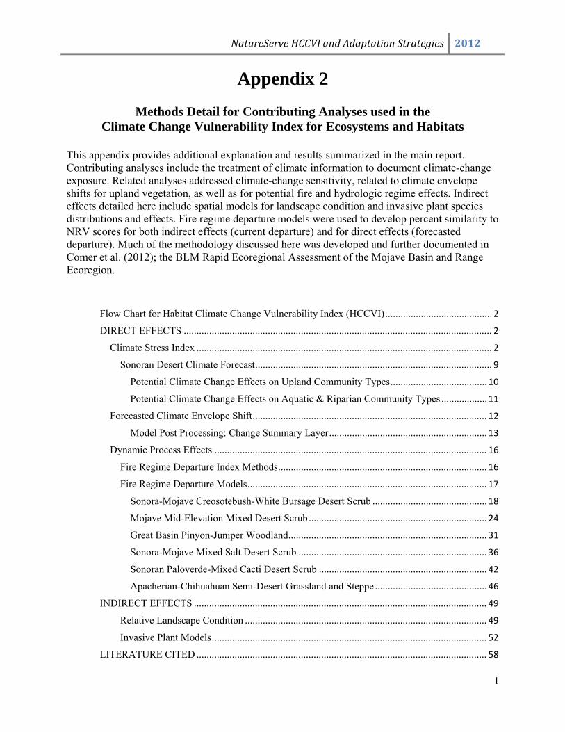
Flow Chart for Habitat Climate Change Vulnerability Index (HCCVI)
Climate Exposure
Climate Stress Index
Envelope Shift Index
Dynamic Process Forecast
Score 0‐1
Score 0‐1
Score 0‐1
Vulnerability
Sensitivity
DIRECT EFFECTS Direct effects were addressed through several indices, depending on the natural characteristics of the community type. Analysis of climate forecasts can provide an indication of the relative intensity of climate-induced stress for temperature and precipitation variables (e.g., increasing temperature relative to precipitation in certain key months). For upland vegetation, climate envelope modeling, correlates current plant community distributions with a suite of key climate variables from a 20th century baseline. The location of this climate envelope in the future in (2050-2059) is then predicted, providing an indication of the directionality, magnitude, and overlap of geographic shift in that envelope. This can also provide insight about successional dynamics and transitions across major vegetation types on the regional landscape. Analysis of fire regime or hydrologic regime may be used to indicate trends in the degree of alteration or ‘departure’ from expected conditions for upland or riparian/aquatic communities. Much of this section is excerpted or adapted from Comer et al. 2012 – BLM Rapid Ecoregional Assessment of the Mojave Basin and Range Ecoregion.
Climate Stress Index Climate forecasts from an ensemble of downscaled global climate models were summarized for the period around 2050-2060. These forecasts indicate the relative degree of forecasted climate stress, using either a comparison of forecasts to 1900-1980 baseline conditions, or more simply, as forecasted change in temperature and precipitation between current and future time periods, gauging the degree of anticipated change on a per-pixel basis.
Very High, High,Moderate, Low
Score 0‐1
Score 0‐1
Indirect EffectsLandscape Condition 1960
Landscape Condition 2010
Direct EffectsClimate Trends
Average
Keystone Species Vuln.
Score 0‐1
Score 0‐1
Score 0‐1
Score 0‐1
Diversity within Plant/Animal Functional Groups
Elevation Range
Adaptive Capacity
Bioclimatic Variability
Invasive Species Effects 1960
Invasive Species Effects 2010 Score 0‐1
Score 0‐1 Sensitivity ScoreLow 0.7-1 Medium 0.5-0.69
High 0.0-0.49
Aver
age
Aver
age
Resilience ScoreHigh 0.7-1
Medium 0.5-0.69Low 0.0-0.49
Score 0‐1Dynamic Process Alteration
HH HM HL
MH MM ML
LH LM LL
Sensitivity
Resi
lienc
e
NatureServe HCCVI and Adaptation Strategies 2012
3
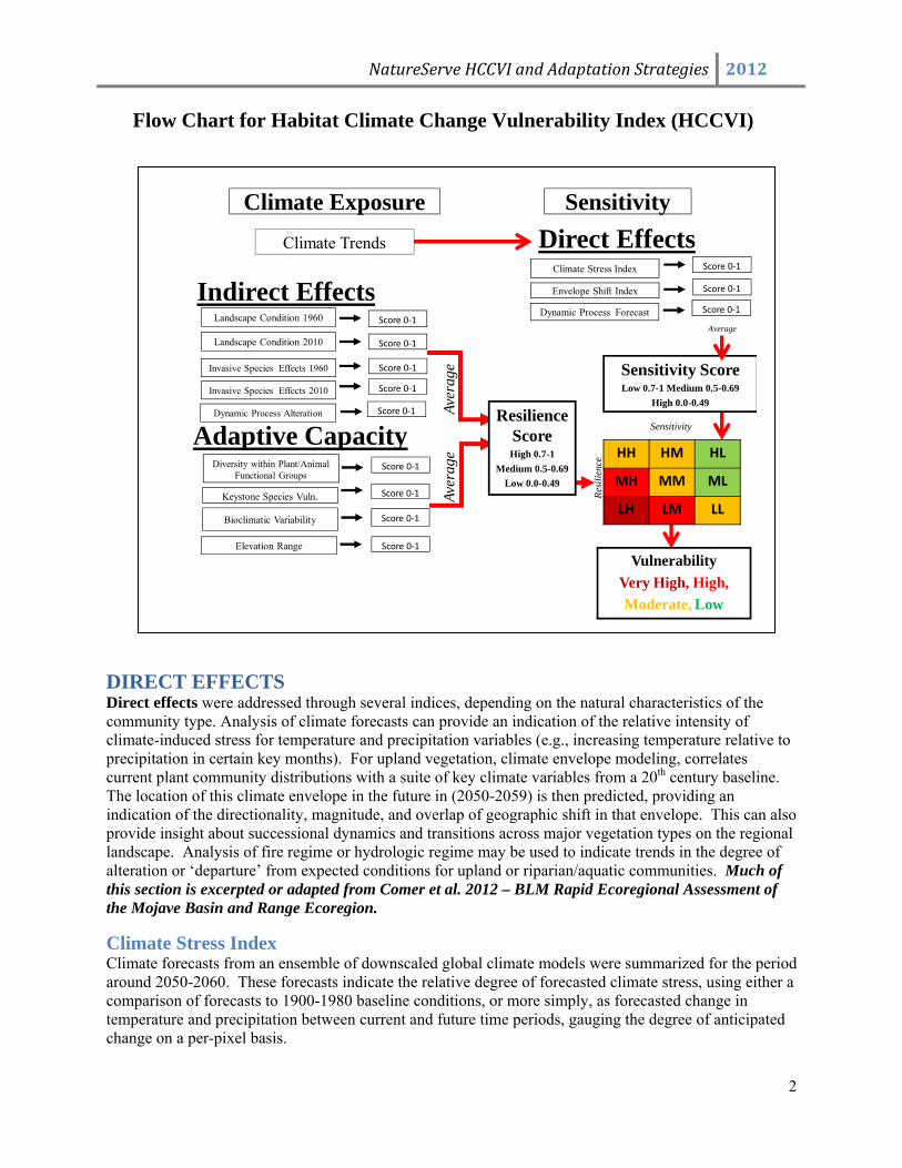
Historical US nationwide climate data were used to characterize a given ecosystem type’s ‘climate envelope’ over the 20th century. For example, PRISM data (http://www.prism.oregonstate.edu/ ) include monthly mean maximum and minimum temperature and mean monthly total precipitation, and are available at 4km2 spatial resolution from 1900 to the present, and 800m resolution since 1950. An analysis of temperature and precipitation variables for the 1900-1980 intervals can characterize “expected” variability and identify historically-stressed conditions (e.g., 1930s drought extremes) that may have occurred prior to the onset of human-induced climate change (1980s). While the relative density of climate stations can affect the quality of PRISM estimates, and these desert landscapes include some of the lowest densities of climate stations in the United States, the interpolation methods deployed for PRISM should be adequate for the our proposed use of the data. An index of climate stress uses statistical analysis to highlight the key climate variables (e.g., monthly maximum and minimum temperatures, and total precipitation. In the Mojave Desert, his index of climate stress was calculated using the weighted average score of the number of climate variables forecasted for 2060 (in a 4km2 grid) when overlain on the current distribution of each community type. The resulting score is calculated as 1 minus % (in decimal) of annual climate variables forecasted to depart >2 stdv from 20th century baseline. For example, up to 12 of 36 monthly variables for maximum temperature, minimum temperature, and total precipitation were forecasted in the Mojave Desert to depart by >2 stdv from the 20th century baseline (Figure A2-1). The number of these significantly departed monthly variables per grid cell formed the basis for weighted averaging. Major communities had weighted averages around 7. In those examples, the resulting index score is therefore 1 – 7/36 = 0.8.
Figure A2-1. The total number of monthly climate variables with significant (2+ stdv change) on a per
pixel basis in Mojave Desert.
NatureServe HCCVI and Adaptation Strategies 2012
4
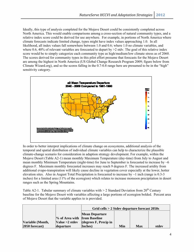
Ideally, this type of analysis completed for the Mojave Desert could be consistently completed across North America. This would enable comparisons among a cross-section of natural community types, and a relative index score could be derived for use anywhere. For example, in portions of North America where climate forecasts indicate limited change, types might have index values approaching 1.0. In all likelihood, all index values fall somewhere between 1.0 and 0.6; where 1.0 no climate variables, and where 0.6, 40% of relevant variables are forecasted to depart by >2 stdv. The goal of this relative index score would be to simply categorize each community type as high/medium/low climate stress as of 2060. The scores derived for community types in this pilot effort presume that forecasts for the Mojave Desert are among the highest in North America (US Global Change Research Program 2009; figure below from Climate Wizard.org), and so the scores falling in the 0.7-0.8 range here are presumed to be in the “high” sensitivity category. In order to better interpret implications of climate change on ecosystems, additional analysis of the temporal and spatial distribution of individual climate variables can help to characterize the plausible climate-change scenario for consideration in adaption strategy development. For example, within the Mojave Desert (Table A2-1) mean monthly Maximum Temperature (day-time) from July to August and mean monthly Minimum Temperature (night-time) for June to September is forecasted to increase by ~6 degrees F. Maximum monthly forecasted increases may reach 9 degrees F. The increased aridity from additional evapo-transpiration will likely cause decline in vegetation cover especially at the lower, hotter elevation sites. Also in August Total Precipitation is forecasted to increase by ~1 inch (range is 0.3-3 inches) for a limited area (11% of the ecoregion) which relates to increase monsoon precipitation in desert ranges such as the Spring Mountains. Table A2-1. Tabular summary of climate variables with > 2 Standard Deviation from 20th Century baseline for the Mojave Desert with variables affecting a large portions of ecoregion bolded. Percent area of Mojave Desert that the variable applies to is provided.
Variable (Month, 2050 forecast)
% of Area with Value >2 stdev departure
Grid cells > 2 Stdev departure forecast 2050s Mean Departure from Baseline (degrees F, Precip in Inches) Min Max stdev
NatureServe HCCVI and Adaptation Strategies 2012
5
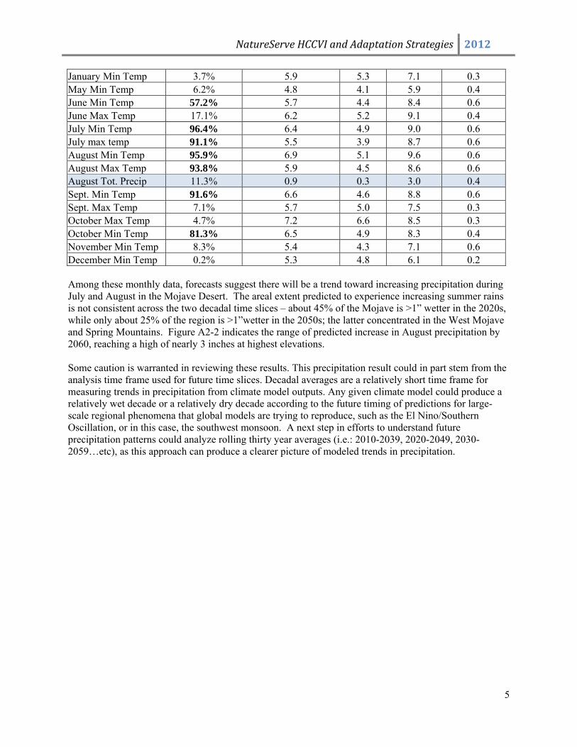
January Min Temp 3.7% 5.9 5.3 7.1 0.3 May Min Temp 6.2% 4.8 4.1 5.9 0.4 June Min Temp 57.2% 5.7 4.4 8.4 0.6 June Max Temp 17.1% 6.2 5.2 9.1 0.4 July Min Temp 96.4% 6.4 4.9 9.0 0.6 July max temp 91.1% 5.5 3.9 8.7 0.6 August Min Temp 95.9% 6.9 5.1 9.6 0.6 August Max Temp 93.8% 5.9 4.5 8.6 0.6 August Tot. Precip 11.3% 0.9 0.3 3.0 0.4 Sept. Min Temp 91.6% 6.6 4.6 8.8 0.6 Sept. Max Temp 7.1% 5.7 5.0 7.5 0.3 October Max Temp 4.7% 7.2 6.6 8.5 0.3 October Min Temp 81.3% 6.5 4.9 8.3 0.4 November Min Temp 8.3% 5.4 4.3 7.1 0.6 December Min Temp 0.2% 5.3 4.8 6.1 0.2 Among these monthly data, forecasts suggest there will be a trend toward increasing precipitation during July and August in the Mojave Desert. The areal extent predicted to experience increasing summer rains is not consistent across the two decadal time slices – about 45% of the Mojave is >1” wetter in the 2020s, while only about 25% of the region is >1”wetter in the 2050s; the latter concentrated in the West Mojave and Spring Mountains. Figure A2-2 indicates the range of predicted increase in August precipitation by 2060, reaching a high of nearly 3 inches at highest elevations. Some caution is warranted in reviewing these results. This precipitation result could in part stem from the analysis time frame used for future time slices. Decadal averages are a relatively short time frame for measuring trends in precipitation from climate model outputs. Any given climate model could produce a relatively wet decade or a relatively dry decade according to the future timing of predictions for large-scale regional phenomena that global models are trying to reproduce, such as the El Nino/Southern Oscillation, or in this case, the southwest monsoon. A next step in efforts to understand future precipitation patterns could analyze rolling thirty year averages (i.e.: 2010-2039, 2020-2049, 2030-2059…etc), as this approach can produce a clearer picture of modeled trends in precipitation.
NatureServe HCCVI and Adaptation Strategies 2012
6
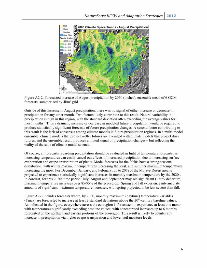
Figure A2-2. Forecasted increase of August precipitation by 2060 (inches); ensemble mean of 6 GCM forecasts, summarized by 4km2 grid Outside of this increase in August precipitation, there was no signal of either increase or decrease in precipitation for any other month. Two factors likely contribute to this result. Natural variability in precipitation is high in this region, with the standard deviation often exceeding the average values for most months. Thus a dramatic increase or decrease in modeled future precipitation would be required to produce statistically significant forecasts of future precipitation changes. A second factor contributing to this result is the lack of consensus among climate models in future precipitation regimes. In a multi-model ensemble, climate models that project wetter futures are averaged with climate models that project drier futures, and the ensemble result produces a muted signal of precipitation changes – but reflecting the reality of the state of climate model science. Of course, all forecasts regarding precipitation should be evaluated in light of temperature forecasts, as increasing temperatures can easily cancel out effects of increased precipitation due to increasing surface evaporation and evapo-transpiration of plants. Model forecasts for the 2050s have a strong seasonal distribution, with winter maximum temperatures increasing the least, and summer maximum temperatures increasing the most. For December, January, and February, up to 20% of the Mojave Desert area is projected to experience statistically significant increases in monthly maximum temperature by the 2020s. In contrast, for this 2020s time period, July, August and September may see significant (1 stdv departure) maximum temperature increases over 85-95% of the ecoregion. Spring and fall experience intermediate amounts of significant maximum temperature increases, with spring projected to be less severe than fall. Figure A2-3 includes forecasts where, by 2060, monthly maximum (daytime) temperature variables (Tmax) are forecasted to increase at least 2 standard deviations above the 20th-century baseline values. As indicated in the figure, everywhere across the ecoregion is forecasted to experience at least one month with temperatures significantly exceeding baseline values; with concentrated increases up to 6 months forecasted on the northern and eastern portions of the ecoregion. This result is likely to counter any increase in precipitation via higher evapo-transpiration and lower soil moisture levels.
NatureServe HCCVI and Adaptation Strategies 2012
7
Figure A2-3. 2060 Climate space trends for monthly Tmax, indicating numbers of months with forecasted Tmax exceeding 20th century baseline mean by > 2 standard deviations; ensemble mean of 6 GCM forecasts, summarized by 4km2 grid By midcentury models predict future summer maximum temperatures will exceed 95% (two standard deviations) of the values that occurred during the 1900-1979 baseline period. March and April are the only two months where less than 90% of the Mojave Desert is projected to experience at least one standard deviation shift in monthly maximum temperatures; by the 2050s, over 91% of the ecoregion will experience at least two standard deviation in July and August monthly maximum temperature (Table A2-1). Change forecasts for 2060 of July maximum temperatures indicate increases varying from less than 2 degrees to 8.6 degrees F (Figure A2-4). These patterns of extreme temperature are generally concentrated in the northern and eastern portions of the ecoregion.
NatureServe HCCVI and Adaptation Strategies 2012
8
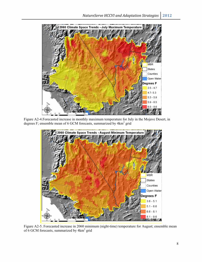
Figure A2-4.Forecasted increase in monthly maximum temperature for July in the Mojave Desert, in degrees F; ensemble mean of 6 GCM forecasts, summarized by 4km2 grid
Figure A2-5. Forecasted increase in 2060 minimum (night-time) temperature for August; ensemble mean of 6 GCM forecasts, summarized by 4km2 grid
NatureServe HCCVI and Adaptation Strategies 2012
9
The increases in monthly minimum temperature (i.e., night-time temperature) are also pervasive and severe. For every month, 85-99% of the Mojave Desert is projected to exceed one standard deviation beyond the 20th century baseline. For midcentury summers – July thru October – models predict 80-95% of the region will experience monthly minimum temperatures two standard deviations beyond baseline values (Table A2-1); with extremes reaching a 9.6 degree F increase (Figure A2-5). This may be related to cloud-cover associated with increased precipitation forecasts; in other words, increased night-time cloud cover will reduce radiative cooling at night. Overall, there is no clear spatial pattern to the area that is not expected to experience these changes, although southern portions more frequently experience values closer to the range of historic climatic variability.
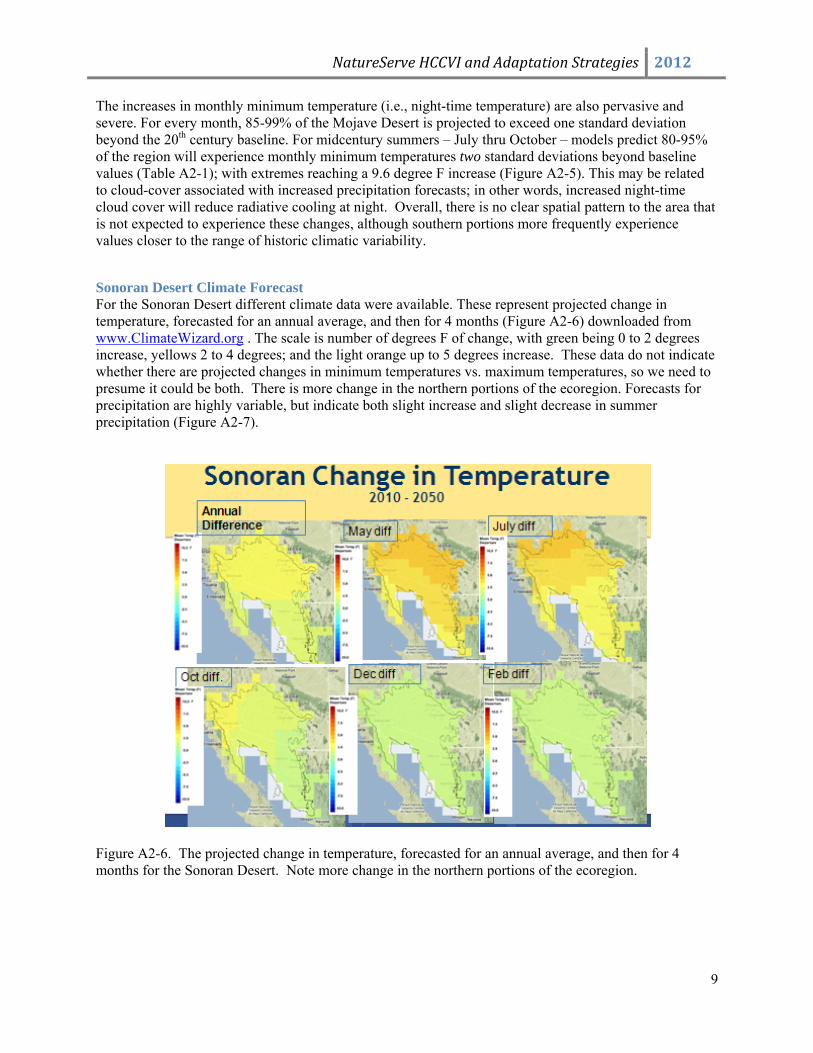
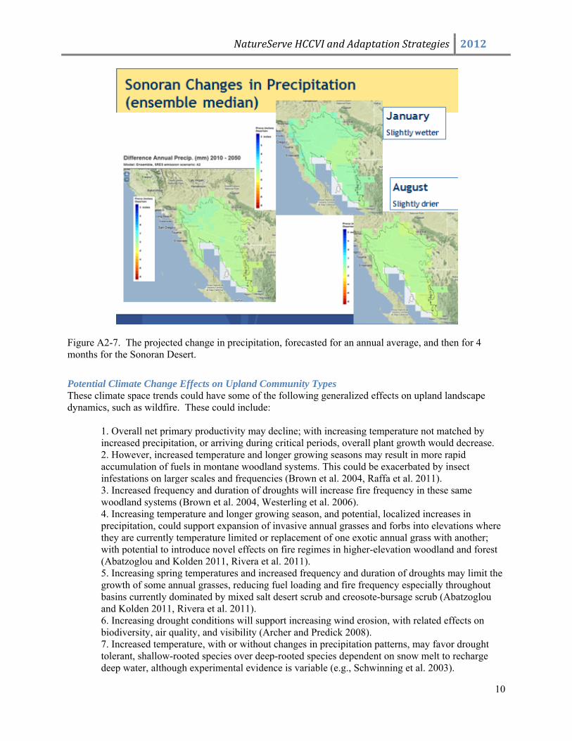
Sonoran Desert Climate Forecast For the Sonoran Desert different climate data were available. These represent projected change in temperature, forecasted for an annual average, and then for 4 months (Figure A2-6) downloaded from www.ClimateWizard.org . The scale is number of degrees F of change, with green being 0 to 2 degrees increase, yellows 2 to 4 degrees; and the light orange up to 5 degrees increase. These data do not indicate whether there are projected changes in minimum temperatures vs. maximum temperatures, so we need to presume it could be both. There is more change in the northern portions of the ecoregion. Forecasts for precipitation are highly variable, but indicate both slight increase and slight decrease in summer precipitation (Figure A2-7).
Figure A2-6. The projected change in temperature, forecasted for an annual average, and then for 4 months for the Sonoran Desert. Note more change in the northern portions of the ecoregion.
NatureServe HCCVI and Adaptation Strategies 2012
10
Figure A2-7. The projected change in precipitation, forecasted for an annual average, and then for 4 months for the Sonoran Desert.
Potential Climate Change Effects on Upland Community Types These climate space trends could have some of the following generalized effects on upland landscape dynamics, such as wildfire. These could include:
1. Overall net primary productivity may decline; with increasing temperature not matched by increased precipitation, or arriving during critical periods, overall plant growth would decrease. 2. However, increased temperature and longer growing seasons may result in more rapid accumulation of fuels in montane woodland systems. This could be exacerbated by insect infestations on larger scales and frequencies (Brown et al. 2004, Raffa et al. 2011). 3. Increased frequency and duration of droughts will increase fire frequency in these same woodland systems (Brown et al. 2004, Westerling et al. 2006). 4. Increasing temperature and longer growing season, and potential, localized increases in precipitation, could support expansion of invasive annual grasses and forbs into elevations where they are currently temperature limited or replacement of one exotic annual grass with another; with potential to introduce novel effects on fire regimes in higher-elevation woodland and forest (Abatzoglou and Kolden 2011, Rivera et al. 2011). 5. Increasing spring temperatures and increased frequency and duration of droughts may limit the growth of some annual grasses, reducing fuel loading and fire frequency especially throughout basins currently dominated by mixed salt desert scrub and creosote-bursage scrub (Abatzoglou and Kolden 2011, Rivera et al. 2011). 6. Increasing drought conditions will support increasing wind erosion, with related effects on biodiversity, air quality, and visibility (Archer and Predick 2008). 7. Increased temperature, with or without changes in precipitation patterns, may favor drought tolerant, shallow-rooted species over deep-rooted species dependent on snow melt to recharge deep water, although experimental evidence is variable (e.g., Schwinning et al. 2003).

NatureServe HCCVI and Adaptation Strategies 2012
11
Potential Climate Change Effects on Aquatic & Riparian Community Types The EcoClim climate space analysis results for the Mojave Desert are not ideal for assessing the impacts of climate change on aquatic communities. These data do not include information on snowpack formation and snowmelt. Although itself a function of temperature and precipitation, snowpack water content (specifically, April 1 Snow Water Equivalent) significantly affects the timing and magnitude of snowmelt within the ecoregion (e.g., Mote 2006, Christensen and Lettenmaier 2007, Das et al. 2009, McCabe and Wolock 2009, Brown and Mote 2009, USBOR 2011). The late-winter/early-spring snowmelt pulse plays an important role in shaping higher-elevation stream hydrology and recharge in the ecoregion. Forecasts of temperature and precipitation therefore provide greater information of relevance to aquatic ecosystems when combined with information on snowpack. The PRISM-EcoClim results provide a first approximation. The spatial patterns discussed above for monthly total precipitation, and monthly maximum/minimum temperatures, provide initial insights for developing adaptation strategies. Specifically, the aquatic communities would be affected by forecasted increases in monthly minimum and maximum temperatures and, to a more limited extent (both spatially and within the year), increases in monthly precipitation. The forecasted changes in temperature are moderate for the 2020s, but become severe for the 2050s. Forecasted changes in July precipitation are mostly moderate across a large portion of the western half of the Mojave Desert for the 2020s, except in the west-central sector of the ecoregion that experience severe departure; and severe for a scattering of locations in the central and northeastern sections of the ecoregion for the 2050s. Forecasted changes in August precipitation are moderate across the entire eastern quarter of the Mojave Desert and most of the entire northwestern quadrant in the 2020s, with small areas of severe departure; and moderate across most of the northwestern quadrant for the 2050s but including a large area of severe departure across the southern Sierra Nevada Range. Increases in precipitation in July and August would involve an increase in the frequency and/or intensity of summer monsoonal storm events. The forecasted changes in temperature and precipitation patterns would be expected to result in several effects on aquatic communities in both the Mojave and Sonoran deserts, as discussed by Melack et al. 1997, Field et al. 1999, Mote 2006, Christensen and Lettenmaier 2007, Chambers and Pellant 2008, Brown and Mote 2009, Covich 2009, Das et al. 2009, Dettinger et al. 2009, McCabe and Wolock 2009, Cayan et al. 2010, Isaak et al. 2010, Miller et al. 2010, and USBOR 2011:
• higher evapo-transpiration rates leading to an earlier, more rapid seasonal (late-winter/spring) drying-down of stream/riparian and lacustrine occurrences;
• increased water stress in basin-floor phreatophyte communities, and seasonally later, less frequent, or briefer wetting of playas;
• shrinkage of areas of perennial flow/open water, coupled with higher water temperatures at locations/times when water temperatures are not controlled by groundwater discharges or snowmelt;
• persistence of these hydrologic conditions later into the fall or early winter; • reduced groundwater recharge in the mountains and reduced recharge to basin-fill deposits
along the mountain-front/basin-fill interface; and • more erosive mid/late summer runoff events in those areas experiencing increased
July/August precipitation, potentially with associated channel down-cutting and expanded deposition of the eroded sediment in lower-elevation gravel fans.
Based on the ways in which these hydrologic factors affect ecological dynamics in the aquatic communities, persistence of these hydro-meteorological impacts over multiple decades could result in several long-term impacts at both high and low elevations, as discussed by many of the authors cited
NatureServe HCCVI and Adaptation Strategies 2012
12
above, and also by, Jager et al. 1999, Harper and Peckarsky 2006, Hultine et al. 2007, Martin 2007, Chambers and Wisdom 2009, Jackson et al. 2009, and Seavy et al. 2009:
• loss of riparian vegetation at lower elevations where the frequency and spatial extent of seasonal flows determines the spatial limits of this vegetation;
• loss of basin-floor phreatophyte (deep-rooted plants that obtain water from ground water sources) communities as a result of lower near-surface ground elevations;
• declines in the spatial extent and biodiversity of perennial streams and open waters as a result of shrinkage and warmer temperatures;
• reduced discharge to springs and seeps as a result of reduced aquifer recharge; • continuation of normal "warm-season" aquatic ecological dynamics later into the fall as a
result of seasonally normal (baseline) overnight near-freezing temperatures becoming less common in many areas until later in the fall; and
• possible de-coupling of the places and timing of emergence of insects, the plants on which they depend, and the animals that feed on the insects, as individual species respond to different cues from air and water temperatures, water availability, and flow conditions.
Forecasted Climate Envelope Shift In order to predict how climate change may shift the suitable climatic conditions for an upland community type, we first define its bioclimatic niche by correlating its current range with current climatic conditions. The vegetation assemblage’s identified niche can then be projected into the future using downscaled Global Circulation Models (GCMs) to predict where a niche will occur at different time slices in 21st century climate scenarios. This information offers one basic building block for a myriad of biogeographic studies that include gauging relative climate change vulnerability. The distribution modeling algorithm MaxEnt (Phillips et al. 2006, Phillips and Dudik 2008) was used in conjunction with spatial climate data from PRISM, EcoClim 4km2 (in USA) and 10km2 (for types with Mexican distribution) data to model current and future bioclimate of each upland community type. MaxEnt is a correlative niche model that uses the principle of maximum entropy to estimate a set of functions that relate environmental variables and known community occurrences in order to approximate a community’s niche and potential geographic distribution (Figure A2-8). MaxEnt was chosen because of its established performance with presence-only data relative to alternative niche modeling techniques, and its built-in capacity to deal with multi-colinearity in the environmental variables (Elith et al. 2006, Elith and Leathwick 2009). MaxEnt is a machine learning algorithm related to Bayesian theory that considers redundant information without penalizing models by over-fitting, eliminating the need to apply any type of variable reduction technique before running the models. MaxEnt calculates a surface of probability across geographic space, where each cell has a value of the probability that a community niche will occur there at a given time. MaxEnt focuses on how the environment where the community is known to occur relates to the environment across the rest of the study area (the “background”). The model does not identify either the community’s occupied niche or fundamental niche; rather the model identifies only that part of the niche defined by the observed records (for further explanation on the algorithm refer to: Phillips et al. 2006, Elith et al. 2011).
Threshold selection In order to translate the raw MaxEnt probability distribution into estimates of community presence or absence, a specific threshold needs to be selected. This is a necessary post-processing step when using an ensemble approach. The threshold used in this analysis is the “equal training sensitivity plus specificity” threshold. This threshold maximizes the agreement between observed and predicted distributions, a
NatureServe HCCVI and Adaptation Strategies 2012
13
choice that has proven to produce the most accurate predictions (Jimenes-Valverde and Lobo 2007; Lobo et al. 2007; Liu et al. 2005).
Model evaluation Model evaluation was performed using the area under the curve (AUC) of the receiver operating characteristic (ROC) plot analysis (Fielding and Bell 1997). Twenty percent of occurrence points for a given conservation element were withheld from the model to be used as independent test data in calculating the AUC. The AUC is a widely accepted, threshold-independent metric of community distribution model performance (Marmion et al., 2009; Warren et al., 2010) that provides an overall picture of how well the data fits the model and has previously been used in comprehensive SDM evaluations (Elith et al. 2006).
Ensemble Approach The ensemble approach focuses on the degree of agreement among multiple GCMs. Various GCMs predict different outcomes for future climatic conditions, even when provided the same input data, because each model accounts for the interactions of various elements of the oceanic-atmospheric system differently. Therefore, an ensemble approach, wherein multiple GCMs are run using the same input data and emissions scenarios and their results compared, averaged, or otherwise aggregated, is increasingly accepted as the preferred method for applying climate projections for a variety of purposes (Tebaldi et al. 2011). Bioclimatic envelope modeling is conducted with a range of GCMs that have been downscaled to 4km2 using a 50-year 20th century baseline derived from PRISM, following the statistical downscaling methods of Tabor & Williams (2010). Each time slice (here, just the decade of the 2050s) was run independently with each of the 6 different GCMs. The six downscaled GCMs are part of a larger spatial future climate dataset called EcoClim (Hamilton et al. in prep), and were selected on the basis of climate variable availability. The six GCMs used here were the only models vetted for the IPCC’s 4th Assessment Report that archived monthly maximum and minimum temperatures, and were all run under the A2 emissions scenario (as required by scope of REA). Below are the names of the 6 GCMs downscaled to 4km2 and used for bioclimatic envelope modeling and climate space trend analysis.
• BCCR_BCM2_0 • CSIRO_MK3_0 • CSIRO_MK3_5 • INMCM3_0 • MIROC3_2_MEDRES • NCAR_CCSM3_0
The probability outputs were then converted to presence absence and then combined using an additive function. Therefore, each time slice for a given community has 6 values, with 6 being the highest level of agreement (all 6 GCMs agree on a community predicted suitable bioclimate) and 1 being the lowest, (only1 GCM predicts suitable bioclimate). This approach supports an assessment of multi-model agreement in projections of bioclimatic shifts.
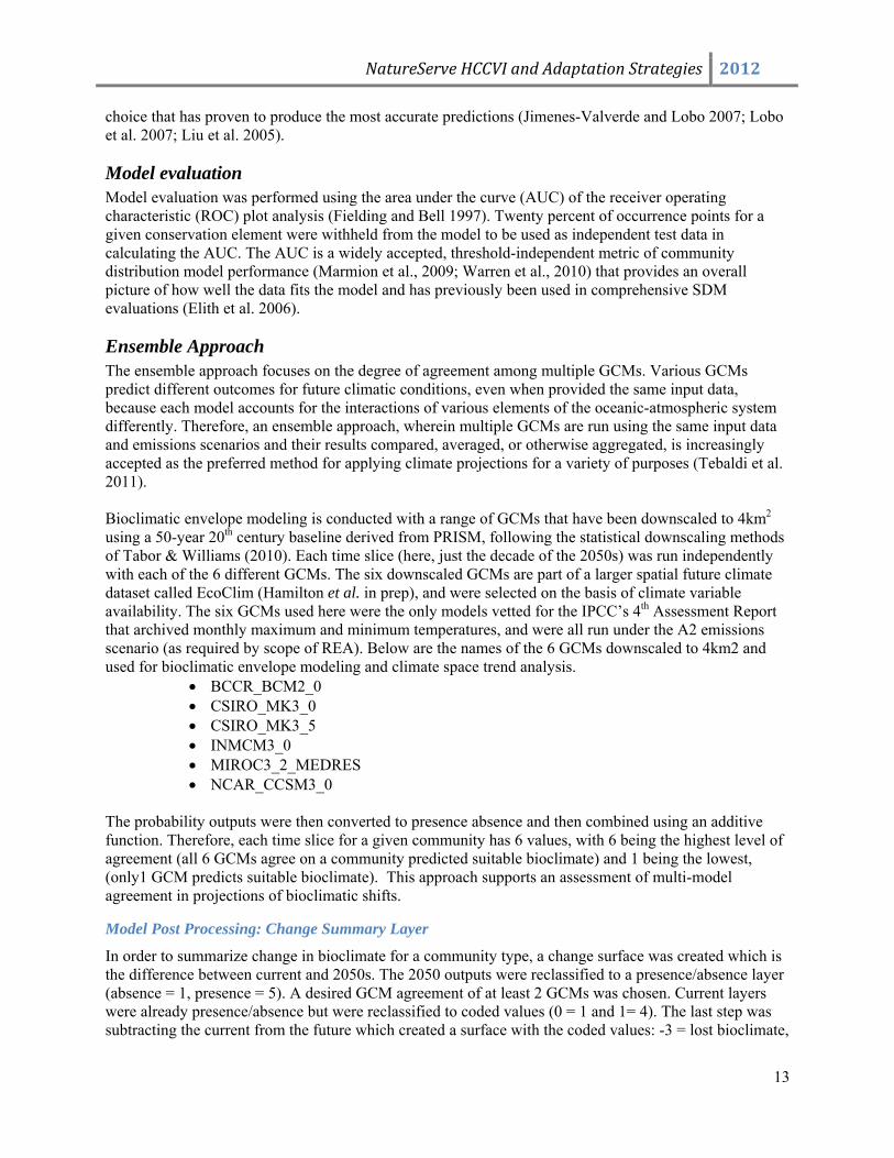
Model Post Processing: Change Summary Layer
In order to summarize change in bioclimate for a community type, a change surface was created which is the difference between current and 2050s. The 2050 outputs were reclassified to a presence/absence layer (absence = 1, presence = 5). A desired GCM agreement of at least 2 GCMs was chosen. Current layers were already presence/absence but were reclassified to coded values (0 = 1 and 1= 4). The last step was subtracting the current from the future which created a surface with the coded values: -3 = lost bioclimate,
NatureServe HCCVI and Adaptation Strategies 2012
14
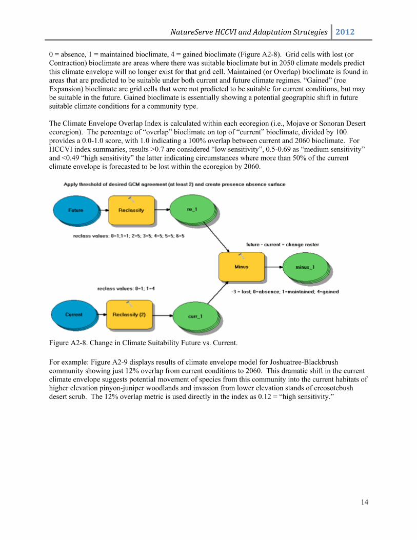
0 = absence, 1 = maintained bioclimate, 4 = gained bioclimate (Figure A2-8). Grid cells with lost (or Contraction) bioclimate are areas where there was suitable bioclimate but in 2050 climate models predict this climate envelope will no longer exist for that grid cell. Maintained (or Overlap) bioclimate is found in areas that are predicted to be suitable under both current and future climate regimes. “Gained” (roe Expansion) bioclimate are grid cells that were not predicted to be suitable for current conditions, but may be suitable in the future. Gained bioclimate is essentially showing a potential geographic shift in future suitable climate conditions for a community type. The Climate Envelope Overlap Index is calculated within each ecoregion (i.e., Mojave or Sonoran Desert ecoregion). The percentage of “overlap” bioclimate on top of “current” bioclimate, divided by 100 provides a 0.0-1.0 score, with 1.0 indicating a 100% overlap between current and 2060 bioclimate. For HCCVI index summaries, results >0.7 are considered “low sensitivity”, 0.5-0.69 as “medium sensitivity” and <0.49 “high sensitivity” the latter indicating circumstances where more than 50% of the current climate envelope is forecasted to be lost within the ecoregion by 2060.
Figure A2-8. Change in Climate Suitability Future vs. Current. For example: Figure A2-9 displays results of climate envelope model for Joshuatree-Blackbrush community showing just 12% overlap from current conditions to 2060. This dramatic shift in the current climate envelope suggests potential movement of species from this community into the current habitats of higher elevation pinyon-juniper woodlands and invasion from lower elevation stands of creosotebush desert scrub. The 12% overlap metric is used directly in the index as 0.12 = “high sensitivity.”
NatureServe HCCVI and Adaptation Strategies 2012
15
Figure A2-9. Climate envelope model for Joshuatree-Blackbrush community showing overlap from current conditions to 2060 using 4 km2 climate data.

NatureServe HCCVI and Adaptation Strategies 2012
16
Dynamic Process Effects Dynamic Regimes: Localized hydrologic or fire regime models for aquatic or upland ecosystems can help account for past alterations and consider projected future climate regimes, applying those estimates to gauge vulnerability. For this project, hydrologic regime dynamics and alterations were treated qualitatively due to a lack of available quantitative/spatial models. However, fire regimes were assessed using available quantitative models. Fire Regime Departure Index Methods
Class I Wildfire For the HCCVI, wildfire was treated by gauging fire regime departure for landscapes supporting a given community type. Fire perimeters up through 2007, in combination with invasive annual grass models (see methods cited below), were used to update LANDFIRE Succession Class (SClass) maps in the Mojave Desert, which had been previously completed using 2000-2002 satellite imagery (see Vogelmann et al. 2011). Similar inputs from the Sonoran Desert REA were used for the US portion of the Sonoran Desert. Fire regime departure information built upon extensive investments by the LANDFIRE effort (see e.g., Keane et al. 2006, Rollins et al. 2006) for both conceptual and spatial modeling for this REA. For each upland community type, a state-and-transition model was developed using the Vegetation Dynamics Development Tool (VDDT) and simulations were run in the Path Landscape Model (ESSA Technologies 2007). Models initially characterize Natural Range of Variation (NRV), and then integrate altered conditions (e.g., invasive plant effects) for forecasting trends. Original LANDFIRE models in portions of the Mojave Desert were updated by the Nevada Chapter of The Nature Conservancy, prior to initiation of that REA. Those for types limited to Sonoran Desert we reviewed and updated for this project. The departure measure used here is the LANDFIRE FRCC Departure Index (FRDI). This indicator gives a summary of how departed the final conditions resulting from each model run are from the reference landscape conditions. It is calculated by comparing the reference percentage of each succession class (SClass) to the percentage resulting from a given model run. In the Mojave Desert, fire regime departure was reported by the 5th-level watershed. For each fire-dependent upland community type, where its areal extent was over 10% of the total watershed area, an estimate of current (and forecasted) fire regime departure was calculated. In the Sonoran Desert, percentages were not evaluated by watershed, but instead were compared for the entire US portion of each community distribution. These calculations compare tabular estimates of NRV Succession Class Distributions against observed SClass distributions from updated LANDFIRE SClass maps for each watershed or other area. This calculation of departure provides a 0-100% score for each community type within the area of interest For application to indirect effects measures, these scores were used directly to indicate relative similarity between NRV and current conditions, using a 0.0-1.0 index range with 1.0 = 100% similarity (= High Resilience). Since SClass maps were updated to approximately 2007 for the REA, information was available to provide new “starting conditions” for simulating a forecasted set of successional proportions out to 2060. While it was infeasible to complete this type of simulation for each 5th level watershed, the predominant 2-5 combinations of current SClass proportions in the Mojave Desert was developed for each type as the basis for these forecasts. For example, for a given community there might be three most-characteristic forms of current SClass proportions, representing minimal, moderate, and more extreme fire regime departure. The SClass combinations most characteristic of those three types are known, and tied to their relevant watersheds today. Once forecasted models were completed for each type/departure combination, their resultant scores were tied back to the relevant watershed for REA reporting. Again, given limitations
NatureServe HCCVI and Adaptation Strategies 2012
17
of available data, one single model run was completed for types across the US portion of the Sonoran Desert. For application to Climate Change Sensitivity measures, the forecasted departure scores for 2060 also indicate relative similarity between NRV and future conditions, using a 0.0-1.0 index range with 1.0 = 100% similarity (= Low Sensitivity). Natural fire regimes in both the Sonoran and Mojave Desert regions have been altered as a result of grazing by domestic livestock, fire suppression, and the introduction and spread of invasive weeds over the last 100 years. The reduction of fine fuels as a result of grazing may allow the presence of relatively fire-intolerant species such as Artemisia tridentata, Coleogyne ramosissima, Larrea tridentata or Pinus monophylla in stands of systems in relatively mesic sites (Keeler-Wolf and Thomas 2000) and their elimination from drier sites. In sites throughout the range of several widespread types, annual grass invasion has also substantially altered the fire frequency. Fine fuel accumulation from alien annual grasses, such as Bromus madritensis, Bromus tectorum, and Schismus spp., currently represents the most important fuelbed component in desert scrub, and substantially increases both fire frequency and fire size. After a year of moderate to high rainfall, cured-out annual vegetation creates dense fine fuels that can carry fire through these open scrub stands, killing fire-sensitive native species and converting the vegetation to exotic annual grasslands (Keeler-Wolf et al. 1998).
Fire Regime Departure Models
In the following pages, each fire regime model used in the HCCVI is described. Fire Regime Departure Model development varied slightly between Mojave Desert and Sonoran Desert pilot community types. Models for Mojave Desert pilot types are modified from LANDFIRE models (Map Zone 14) and from models produced for the Nevada Strategic Wildlife Action Plan (SWAP) (Provencher 2011) for the Mojave Desert BLM Rapid Ecological Assessment (REA) so additional REA information is provided for this effort. Whereas models for Sonoran Desert pilot upland systems are modified from LANDFIRE models (Map Zone 13). Models display both states and transitions within Natural Range of Variation (NRV) and uncharacteristic states.
NatureServe HCCVI and Adaptation Strategies 2012
18
Sonora-Mojave Creosotebush-White Bursage Desert Scrub This system covers vast areas of sandy alluvial fans, bajadas and rocky slopes in the northwestern Sonoran, Mojave and Colorado deserts (Keeler-Wolf 2007, Sawyer et al. 2009). The dominant shrub, Larrea tridentata, is very long-lived, with clones living >10,000 years (Keeler-Wolf 2007), and is very tolerant of drought and high temperatures. L. tridentata has with small, evergreen, resinous (highly flammable) leaves reducing evapo-transpiration (Hamerlynck et al. 2002). It may die-back during extreme drought, but can sprout from the base (Meinzer et al. 1990). It has low recruitment and is slow to re-establish from seed (Keeler-Wolf 2007). The main codominant shrub, Ambrosia dumosa, is short-lived with a relatively shallow root system, and tends to dominate sandy and rocky sites. It can quickly establish after disturbance or drought (Vasek 1980). Post fire, it has a limited ability to sprout, but will re-establish from seed (Sawyer et al. 2009). Fire-return interval for this typically open-canopied shrub system is long to truncated long. When it burns, fires have high intensity and moderate severity (Sawyer et al. 2009). Fires in historic creosote-bursage stands are thought to have been infrequent except along the margins of the occurrence where it mixed with shrub-steppe containing greater grass fuel loading. Although bunch grasses can fill in some of the interspaces between shrubs with fine fuels, their distribution is generally patchy and rarely provides fuel continuity sufficient to carry fire (Brooks et al. 2007). Periodic drought is occasionally sufficient to thin grass and shrub cover.
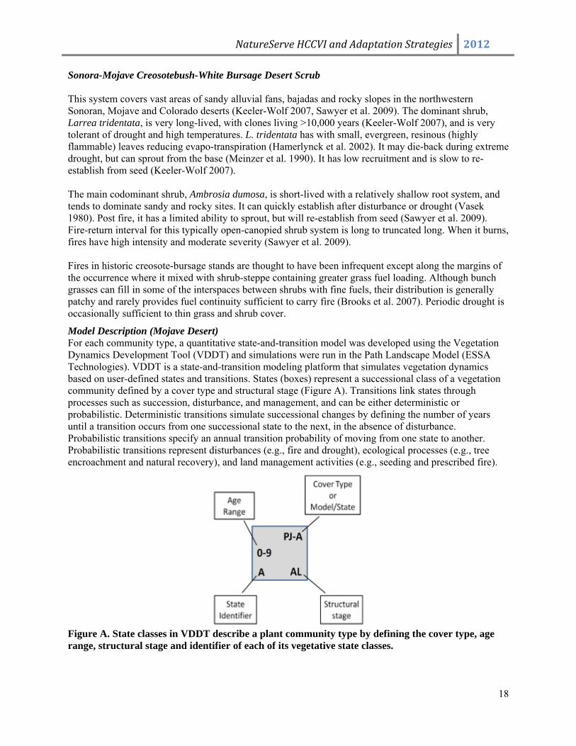
Model Description (Mojave Desert) For each community type, a quantitative state-and-transition model was developed using the Vegetation Dynamics Development Tool (VDDT) and simulations were run in the Path Landscape Model (ESSA Technologies). VDDT is a state-and-transition modeling platform that simulates vegetation dynamics based on user-defined states and transitions. States (boxes) represent a successional class of a vegetation community defined by a cover type and structural stage (Figure A). Transitions link states through processes such as succession, disturbance, and management, and can be either deterministic or probabilistic. Deterministic transitions simulate successional changes by defining the number of years until a transition occurs from one successional state to the next, in the absence of disturbance. Probabilistic transitions specify an annual transition probability of moving from one state to another. Probabilistic transitions represent disturbances (e.g., fire and drought), ecological processes (e.g., tree encroachment and natural recovery), and land management activities (e.g., seeding and prescribed fire).
Figure A. State classes in VDDT describe a plant community type by defining the cover type, age range, structural stage and identifier of each of its vegetative state classes.
NatureServe HCCVI and Adaptation Strategies 2012
19
For each simulation, the landscape is partitioned into a number of cells or simulation units and allocated among state classes in the model. At each time step, deterministic transitions occur based on the age of the cell and probabilistic transitions may occur based on the specified transition probability. VDDT is a nonspatial model, and all cells are simulated independently of other cells. The Path tool uses VDDT as a simulation engine but allows users to organize model runs, run many models simultaneously, and view output across all model runs simultaneously. Each community type was described using two VDDT models – one describing the natural range of variation (NRV) under historic conditions, and one describing contemporary dynamics and including uncharacteristic states such as annual grass or depleted shrub. The contemporary model includes all states and transitions from the NRV model in addition to a set of uncharacteristic states and transitions.
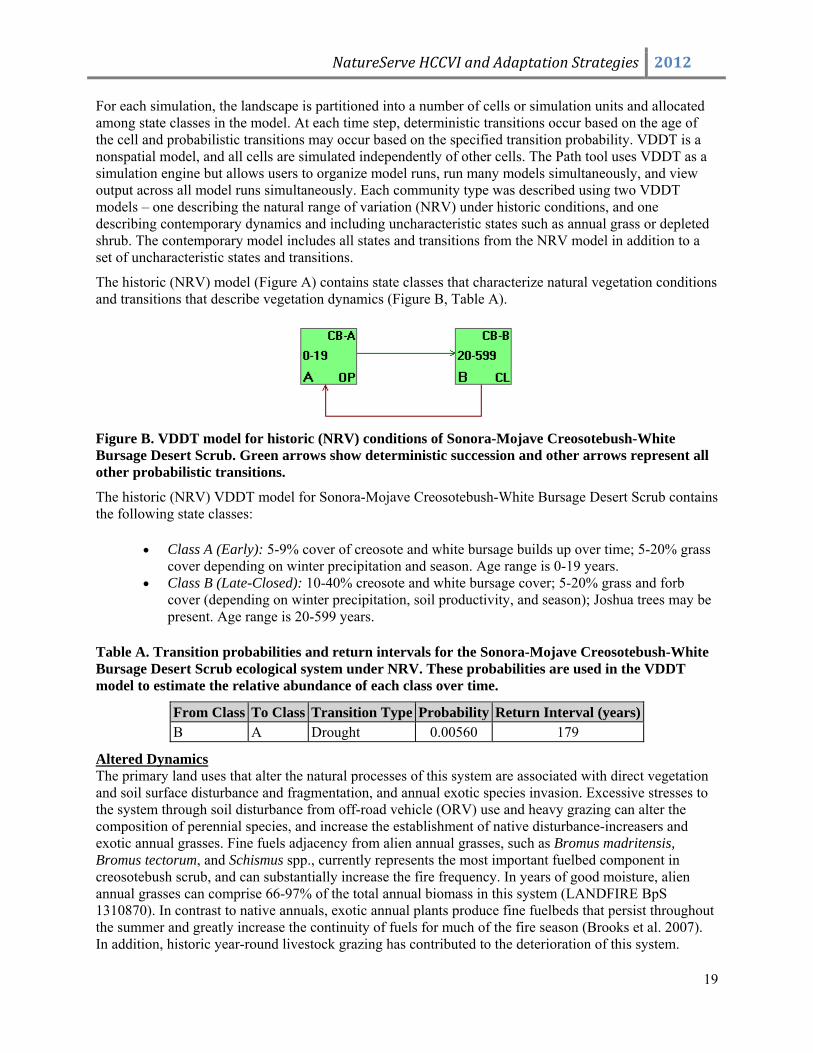
The historic (NRV) model (Figure A) contains state classes that characterize natural vegetation conditions and transitions that describe vegetation dynamics (Figure B, Table A).
Figure B. VDDT model for historic (NRV) conditions of Sonora-Mojave Creosotebush-White Bursage Desert Scrub. Green arrows show deterministic succession and other arrows represent all other probabilistic transitions.
The historic (NRV) VDDT model for Sonora-Mojave Creosotebush-White Bursage Desert Scrub contains the following state classes:
• Class A (Early): 5-9% cover of creosote and white bursage builds up over time; 5-20% grass cover depending on winter precipitation and season. Age range is 0-19 years.
• Class B (Late-Closed): 10-40% creosote and white bursage cover; 5-20% grass and forb cover (depending on winter precipitation, soil productivity, and season); Joshua trees may be present. Age range is 20-599 years.
Table A. Transition probabilities and return intervals for the Sonora-Mojave Creosotebush-White Bursage Desert Scrub ecological system under NRV. These probabilities are used in the VDDT model to estimate the relative abundance of each class over time.
From Class To Class Transition Type Probability Return Interval (years) B A Drought 0.00560 179
Altered Dynamics The primary land uses that alter the natural processes of this system are associated with direct vegetation and soil surface disturbance and fragmentation, and annual exotic species invasion. Excessive stresses to the system through soil disturbance from off-road vehicle (ORV) use and heavy grazing can alter the composition of perennial species, and increase the establishment of native disturbance-increasers and exotic annual grasses. Fine fuels adjacency from alien annual grasses, such as Bromus madritensis, Bromus tectorum, and Schismus spp., currently represents the most important fuelbed component in creosotebush scrub, and can substantially increase the fire frequency. In years of good moisture, alien annual grasses can comprise 66-97% of the total annual biomass in this system (LANDFIRE BpS 1310870). In contrast to native annuals, exotic annual plants produce fine fuelbeds that persist throughout the summer and greatly increase the continuity of fuels for much of the fire season (Brooks et al. 2007). In addition, historic year-round livestock grazing has contributed to the deterioration of this system.
NatureServe HCCVI and Adaptation Strategies 2012
20
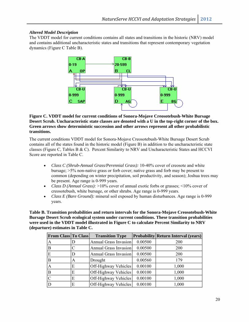
Altered Model Description The VDDT model for current conditions contains all states and transitions in the historic (NRV) model and contains additional uncharacteristic states and transitions that represent contemporary vegetation dynamics (Figure C Table B).
Figure C. VDDT model for current conditions of Sonora-Mojave Creosotebush-White Bursage Desert Scrub. Uncharacteristic state classes are denoted with a U in the top-right corner of the box. Green arrows show deterministic succession and other arrows represent all other probabilistic transitions.
The current conditions VDDT model for Sonora-Mojave Creosotebush-White Bursage Desert Scrub contains all of the states found in the historic model (Figure B) in addition to the uncharacteristic state classes (Figure C, Tables B & C). Percent Similarity to NRV and Uncharacteristic States and HCCVI Score are reported in Table C.
• Class C (Shrub-Annual Grass/Perennial Grass): 10-40% cover of creosote and white bursage; >5% non-native grass or forb cover; native grass and forb may be present to common (depending on winter precipitation, soil productivity, and season); Joshua trees may be present. Age range is 0-999 years.
• Class D (Annual Grass): >10% cover of annual exotic forbs or grasses; <10% cover of creosotebush, white bursage, or other shrubs. Age range is 0-999 years.
• Class E (Bare Ground): mineral soil exposed by human disturbances. Age range is 0-999 years.
Table B. Transition probabilities and return intervals for the Sonora-Mojave Creosotebush-White Bursage Desert Scrub ecological system under current conditions. These transition probabilities were used in the VDDT model illustrated in Figure C to calculate Percent Similarity to NRV (departure) estimates in Table C.
From Class To Class Transition Type Probability Return Interval (years)A D Annual Grass Invasion 0.00500 200 B C Annual Grass Invasion 0.00500 200 E D Annual Grass Invasion 0.00500 200 B A Drought 0.00560 179 A E Off-Highway Vehicles 0.00100 1,000 B E Off-Highway Vehicles 0.00100 1,000 C E Off-Highway Vehicles 0.00100 1,000 D E Off-Highway Vehicles 0.00100 1,000
NatureServe HCCVI and Adaptation Strategies 2012
21
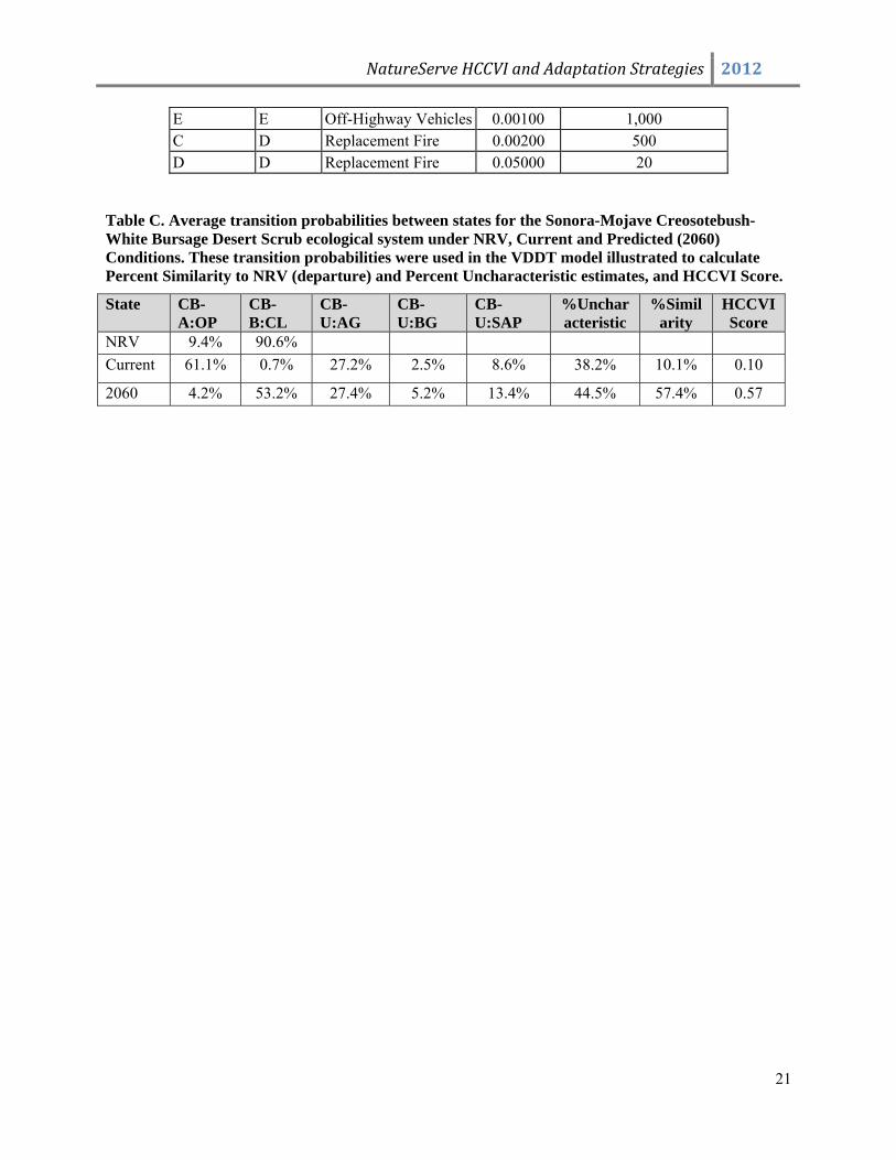
E E Off-Highway Vehicles 0.00100 1,000 C D Replacement Fire 0.00200 500 D D Replacement Fire 0.05000 20
Table C. Average transition probabilities between states for the Sonora-Mojave Creosotebush-White Bursage Desert Scrub ecological system under NRV, Current and Predicted (2060) Conditions. These transition probabilities were used in the VDDT model illustrated to calculate Percent Similarity to NRV (departure) and Percent Uncharacteristic estimates, and HCCVI Score.
State CB-A:OP
CB-B:CL
CB-U:AG
CB-U:BG
CB-U:SAP
%Uncharacteristic
%Similarity
HCCVI Score
NRV 9.4% 90.6% Current 61.1% 0.7% 27.2% 2.5% 8.6% 38.2% 10.1% 0.10
2060 4.2% 53.2% 27.4% 5.2% 13.4% 44.5% 57.4% 0.57
NatureServe HCCVI and Adaptation Strategies 2012
22
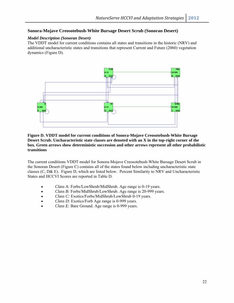
Sonora-Mojave Creosotebush-White Bursage Desert Scrub (Sonoran Desert) Model Description (Sonoran Desert) The VDDT model for current conditions contains all states and transitions in the historic (NRV) and additional uncharacteristic states and transitions that represent Current and Future (2060) vegetation dynamics (Figure D).
Figure D. VDDT model for current conditions of Sonora-Mojave Creosotebush-White Bursage Desert Scrub. Uncharacteristic state classes are denoted with an X in the top-right corner of the box. Green arrows show deterministic succession and other arrows represent all other probabilistic transitions
The current conditions VDDT model for Sonora-Mojave Creosotebush-White Bursage Desert Scrub in the Sonoran Desert (Figure C) contains all of the states found below including uncharacteristic state classes (C, D& E). Figure D, which are listed below. Percent Similarity to NRV and Uncharacteristic States and HCCVI Scores are reported in Table D.
• Class A: Forbs/LowShrub/MidShrub. Age range is 0-19 years. • Class B: Forbs/MidShrub/LowShrub. Age range is 20-999 years. • Class C: Exotics/Forbs/MidShrub/LowShrub 0-19 years. • Class D: Exotics/Forb Age range is 0-999 years. • Class E: Bare Ground. Age range is 0-999 years.
NatureServe HCCVI and Adaptation Strategies 2012
23
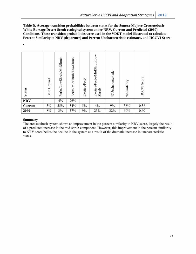
Table D. Average transition probabilities between states for the Sonora-Mojave Creosotebush-White Bursage Desert Scrub ecological system under NRV, Current and Predicted (2060) Conditions. These transition probabilities were used in the VDDT model illustrated to calculate Percent Similarity to NRV (departure) and Percent Uncharacteristic estimates, and HCCVI Score
.
Stat
es
Bar
e G
roun
d
Forb
s/Lo
wSh
rub/
Mid
Shru
b
Forb
s/M
idSh
rub/
Low
Shru
b
Exot
ics/
Forb
Exot
ics/
Forb
s/M
idSh
rub/
Low
Shru
b
%U
ncha
ract
eris
tic
%Si
mila
rity
HC
CV
I Sco
re
NRV 4% 96% Current 3% 55% 34% 5% 4% 9% 38% 0.38 2060 8% 3% 57% 9% 23% 32% 60% 0.60 Summary The creosotebush system shows an improvement in the percent similarity to NRV score, largely the result of a predicted increase in the mid-shrub component. However, this improvement in the percent similarity to NRV score belies the decline in the system as a result of the dramatic increase in uncharacteristic states.
NatureServe HCCVI and Adaptation Strategies 2012
24
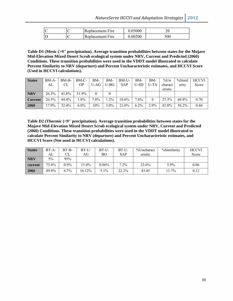
Mojave Mid-Elevation Mixed Desert Scrub Disturbance dynamics in this community type are variable because of variation in structure and composition, being dominated by open- to closed-canopy scrub to desert grasslands dominated by Pleuraphis rigida (<1400 m elevation) and Pleuraphis jamesii (>1400 m elevation) sometimes with a Yucca brevifolia overstory (Sawyer et al. 2009). Except for the relatively few stands with an herbaceous layer, fire-return intervals (FRI) also tend to be long because the open stands only burn under extreme conditions. Older Yucca brevifolia individuals can tolerate low-severity fires due to fire-resistant bark, and both Yucca brevifolia and Yucca schidigera can resprout if burned (Gucker 2006a, 2006b). However, fire-sensitive shrub species such as the long-lived Coleogyne ramosissima, Menodora spinescens, Nolina bigelovii, or Nolina parryi will convert to ruderal and intermediate shrublands dominated by Hymenoclea salsola (= Ambrosia salsola), Grayia spinosa, Gutierrezia sarothrae, Ephedra nevadensis, Ericameria teretifolia, Menodora spinescens, Opuntia acanthocarpa, Salazaria mexicana, Tetradymia spp., or Yucca schidigera which have shorter FRIs (Anderson 2001c, Keeler-Wolf 2007, Sawyer et al. 2009).
Model Description (Mojave Desert) Two models for this system were created to represent a warmer, thermic version (<9 inches precipitation) and the more widespread, more typical mesic version (>9 inches precipitation). Both models were provided, but only the mesic model was used in the HCCVI.
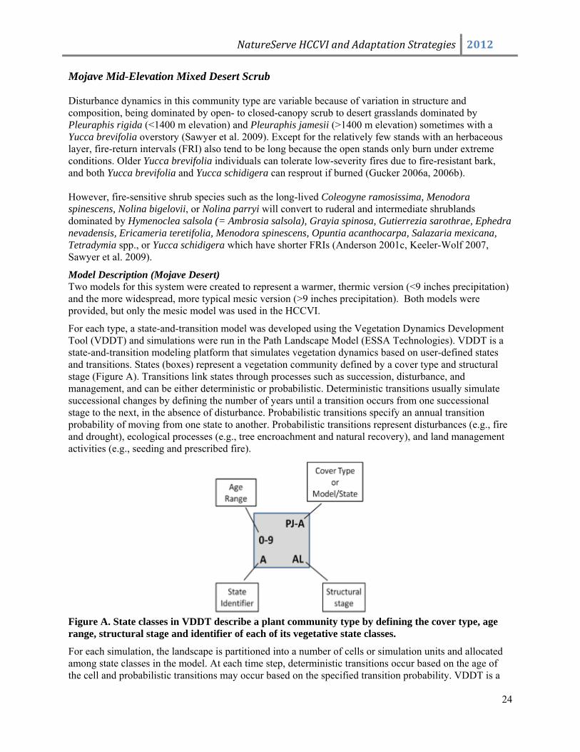
For each type, a state-and-transition model was developed using the Vegetation Dynamics Development Tool (VDDT) and simulations were run in the Path Landscape Model (ESSA Technologies). VDDT is a state-and-transition modeling platform that simulates vegetation dynamics based on user-defined states and transitions. States (boxes) represent a vegetation community defined by a cover type and structural stage (Figure A). Transitions link states through processes such as succession, disturbance, and management, and can be either deterministic or probabilistic. Deterministic transitions usually simulate successional changes by defining the number of years until a transition occurs from one successional stage to the next, in the absence of disturbance. Probabilistic transitions specify an annual transition probability of moving from one state to another. Probabilistic transitions represent disturbances (e.g., fire and drought), ecological processes (e.g., tree encroachment and natural recovery), and land management activities (e.g., seeding and prescribed fire).
Figure A. State classes in VDDT describe a plant community type by defining the cover type, age range, structural stage and identifier of each of its vegetative state classes.
For each simulation, the landscape is partitioned into a number of cells or simulation units and allocated among state classes in the model. At each time step, deterministic transitions occur based on the age of the cell and probabilistic transitions may occur based on the specified transition probability. VDDT is a
NatureServe HCCVI and Adaptation Strategies 2012
25
nonspatial model, and all cells are simulated independently of other cells. The Path model uses VDDT as a simulation engine but allows users to organize model runs, run many models simultaneously, and view output across all model runs simultaneously. Each coarse-filter CE was described using two VDDT models – one describing the natural range of variation (NRV) under historic conditions, and one describing contemporary dynamics and including uncharacteristic states such as annual grass or depleted shrub. The contemporary model includes all states and transitions from the NRV model in addition to a set of uncharacteristic states and transitions .
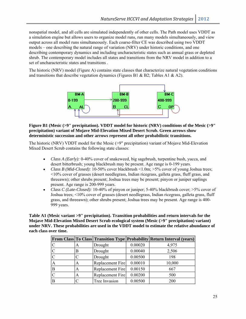
The historic (NRV) model (Figure A) contains state classes that characterize natural vegetation conditions and transitions that describe vegetation dynamics (Figures B1 & B2; Tables A1 & A2).
Figure B1 (Mesic (>9" precipitation). VDDT model for historic (NRV) conditions of the Mesic (>9" precipitation) variant of Mojave Mid-Elevation Mixed Desert Scrub. Green arrows show deterministic succession and other arrows represent all other probabilistic transitions.
The historic (NRV) VDDT model for the Mesic (>9" precipitation) variant of Mojave Mid-Elevation Mixed Desert Scrub contains the following state classes:
• Class A (Early): 0-40% cover of snakeweed, big sagebrush, turpentine bush, yucca, and desert bitterbrush; young blackbrush may be present. Age range is 0-199 years.
• Class B (Mid-Closed): 10-50% cover blackbrush <1.0m; >5% cover of young Joshua trees; <10% cover of grasses (desert needlegrass, Indian ricegrass, galleta grass, fluff grass, and threeawn); other shrubs present; Joshua trees may be present; pinyon or juniper saplings present. Age range is 200-999 years.
• Class C (Late-Closed): 10-40% of pinyon or juniper; 5-40% blackbrush cover; >5% cover of Joshua trees; <10% cover of grasses (desert needlegrass, Indian ricegrass, galleta grass, fluff grass, and threeawn); other shrubs present; Joshua trees may be present. Age range is 400-999 years.
Table A1 (Mesic variant >9" precipitation). Transition probabilities and return intervals for the Mojave Mid-Elevation Mixed Desert Scrub ecological system (Mesic (>9" precipitation) variant) under NRV. These probabilities are used in the VDDT model to estimate the relative abundance of each class over time.
From Class To Class Transition Type Probability Return Interval (years) C A Drought 0.00020 4,975 C B Drought 0.00040 2,506 C C Drought 0.00500 198 A A Replacement Fire 0.00010 10,000 B A Replacement Fire 0.00150 667 C A Replacement Fire 0.00200 500 B C Tree Invasion 0.00500 200
NatureServe HCCVI and Adaptation Strategies 2012
26
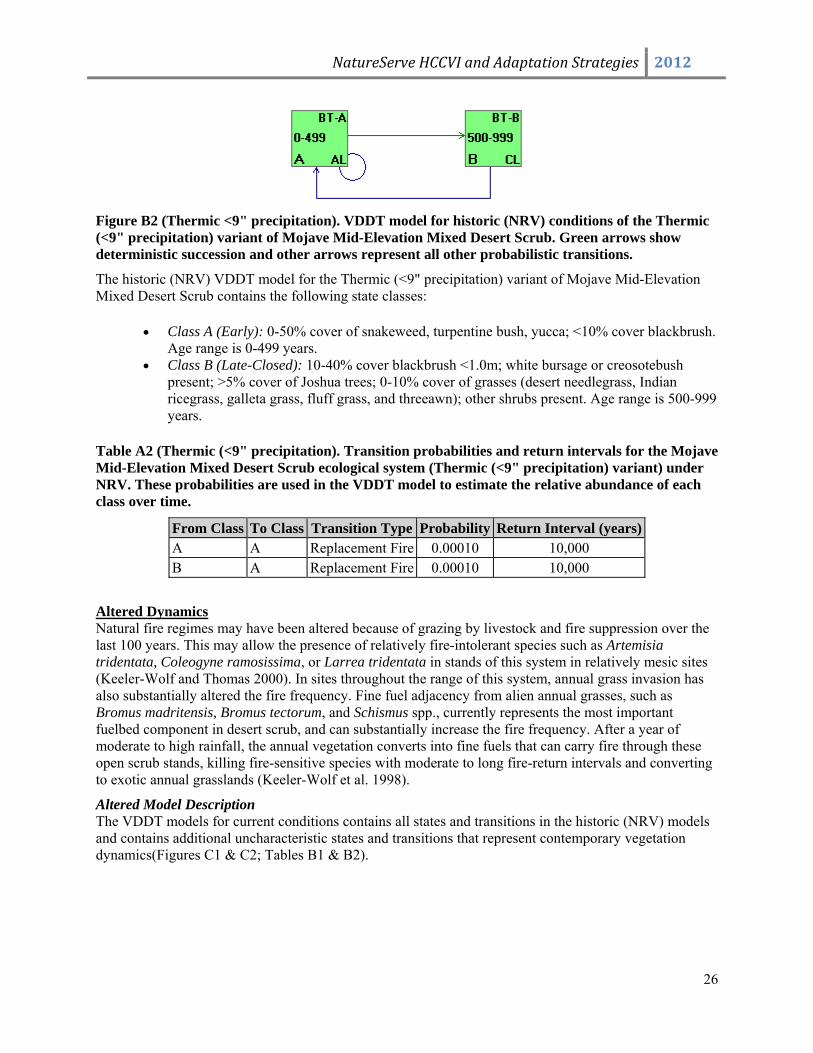
Figure B2 (Thermic <9" precipitation). VDDT model for historic (NRV) conditions of the Thermic (<9" precipitation) variant of Mojave Mid-Elevation Mixed Desert Scrub. Green arrows show deterministic succession and other arrows represent all other probabilistic transitions.
The historic (NRV) VDDT model for the Thermic (<9" precipitation) variant of Mojave Mid-Elevation Mixed Desert Scrub contains the following state classes:
• Class A (Early): 0-50% cover of snakeweed, turpentine bush, yucca; <10% cover blackbrush. Age range is 0-499 years.
• Class B (Late-Closed): 10-40% cover blackbrush <1.0m; white bursage or creosotebush present; >5% cover of Joshua trees; 0-10% cover of grasses (desert needlegrass, Indian ricegrass, galleta grass, fluff grass, and threeawn); other shrubs present. Age range is 500-999 years.
Table A2 (Thermic (<9" precipitation). Transition probabilities and return intervals for the Mojave Mid-Elevation Mixed Desert Scrub ecological system (Thermic (<9" precipitation) variant) under NRV. These probabilities are used in the VDDT model to estimate the relative abundance of each class over time.
From Class To Class Transition Type Probability Return Interval (years) A A Replacement Fire 0.00010 10,000 B A Replacement Fire 0.00010 10,000
Altered Dynamics Natural fire regimes may have been altered because of grazing by livestock and fire suppression over the last 100 years. This may allow the presence of relatively fire-intolerant species such as Artemisia tridentata, Coleogyne ramosissima, or Larrea tridentata in stands of this system in relatively mesic sites (Keeler-Wolf and Thomas 2000). In sites throughout the range of this system, annual grass invasion has also substantially altered the fire frequency. Fine fuel adjacency from alien annual grasses, such as Bromus madritensis, Bromus tectorum, and Schismus spp., currently represents the most important fuelbed component in desert scrub, and can substantially increase the fire frequency. After a year of moderate to high rainfall, the annual vegetation converts into fine fuels that can carry fire through these open scrub stands, killing fire-sensitive species with moderate to long fire-return intervals and converting to exotic annual grasslands (Keeler-Wolf et al. 1998).
Altered Model Description The VDDT models for current conditions contains all states and transitions in the historic (NRV) models and contains additional uncharacteristic states and transitions that represent contemporary vegetation dynamics(Figures C1 & C2; Tables B1 & B2).
NatureServe HCCVI and Adaptation Strategies 2012
27
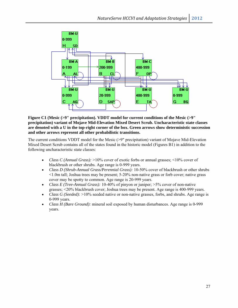
Figure C1 (Mesic (>9" precipitation). VDDT model for current conditions of the Mesic (>9" precipitation) variant of Mojave Mid-Elevation Mixed Desert Scrub. Uncharacteristic state classes are denoted with a U in the top-right corner of the box. Green arrows show deterministic succession and other arrows represent all other probabilistic transitions.
The current conditions VDDT model for the Mesic (>9" precipitation) variant of Mojave Mid-Elevation Mixed Desert Scrub contains all of the states found in the historic model (Figures B1) in addition to the following uncharacteristic state classes:
• Class C (Annual Grass): >10% cover of exotic forbs or annual grasses; <10% cover of blackbrush or other shrubs. Age range is 0-999 years.
• Class D (Shrub-Annual Grass/Perennial Grass): 10-50% cover of blackbrush or other shrubs <1.0m tall; Joshua trees may be present; 5-20% non-native grass or forb cover; native grass cover may be spotty to common. Age range is 20-999 years.
• Class E (Tree-Annual Grass): 10-40% of pinyon or juniper; >5% cover of non-native grasses; <20% blackbrush cover; Joshua trees may be present. Age range is 400-999 years.
• Class G (Seeded): >10% seeded native or non-native grasses, forbs, and shrubs. Age range is 0-999 years.
• Class H (Bare Ground): mineral soil exposed by human disturbances. Age range is 0-999 years.
NatureServe HCCVI and Adaptation Strategies 2012
28
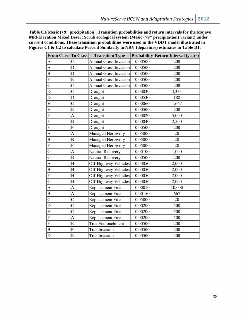
Table C1(Mesic (>9" precipitation). Transition probabilities and return intervals for the Mojave Mid-Elevation Mixed Desert Scrub ecological system (Mesic (>9" precipitation) variant) under current conditions. These transition probabilities were used in the VDDT model illustrated in Figures C1 & C2 to calculate Percent Similarity to NRV (departure) estimates in Table D1.
From Class To Class Transition Type Probability Return Interval (years)A C Annual Grass Invasion 0.00500 200 A D Annual Grass Invasion 0.00500 200 B D Annual Grass Invasion 0.00500 200 F E Annual Grass Invasion 0.00500 200 G C Annual Grass Invasion 0.00500 200 D C Drought 0.00030 3,333 D D Drought 0.00530 188 E C Drought 0.00060 1,667 E E Drought 0.00500 200 F A Drought 0.00020 5,000 F B Drought 0.00040 2,500 F F Drought 0.00500 200 A A Managed Herbivory 0.05000 20 B B Managed Herbivory 0.05000 20 F F Managed Herbivory 0.05000 20 G A Natural Recovery 0.00100 1,000 G B Natural Recovery 0.00500 200 A H Off-Highway Vehicles 0.00050 2,000 B H Off-Highway Vehicles 0.00050 2,000 F H Off-Highway Vehicles 0.00050 2,000 G H Off-Highway Vehicles 0.00050 2,000 A A Replacement Fire 0.00010 10,000 B A Replacement Fire 0.00150 667 C C Replacement Fire 0.05000 20 D C Replacement Fire 0.00200 500 E C Replacement Fire 0.00200 500 F A Replacement Fire 0.00200 500 F E Tree Encroachment 0.00500 200 B F Tree Invasion 0.00500 200 D E Tree Invasion 0.00500 200
NatureServe HCCVI and Adaptation Strategies 2012
29
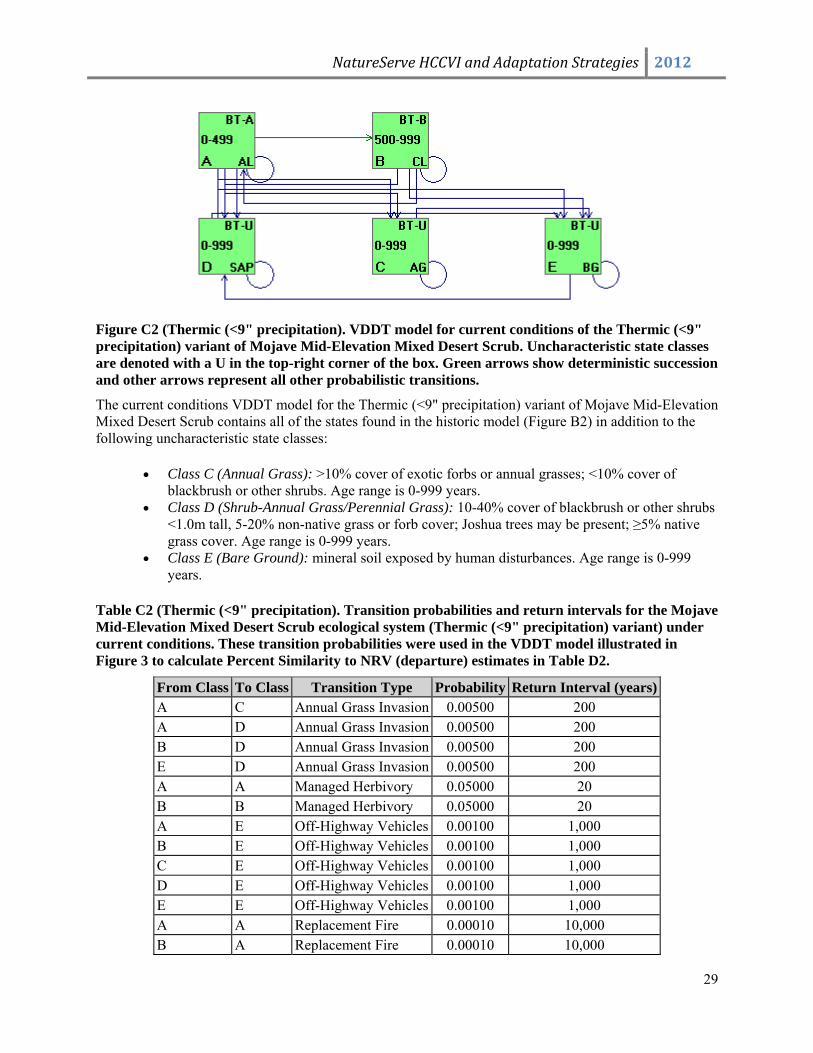
Figure C2 (Thermic (<9" precipitation). VDDT model for current conditions of the Thermic (<9" precipitation) variant of Mojave Mid-Elevation Mixed Desert Scrub. Uncharacteristic state classes are denoted with a U in the top-right corner of the box. Green arrows show deterministic succession and other arrows represent all other probabilistic transitions.
The current conditions VDDT model for the Thermic (<9" precipitation) variant of Mojave Mid-Elevation Mixed Desert Scrub contains all of the states found in the historic model (Figure B2) in addition to the following uncharacteristic state classes:
• Class C (Annual Grass): >10% cover of exotic forbs or annual grasses; <10% cover of blackbrush or other shrubs. Age range is 0-999 years.
• Class D (Shrub-Annual Grass/Perennial Grass): 10-40% cover of blackbrush or other shrubs <1.0m tall, 5-20% non-native grass or forb cover; Joshua trees may be present; ≥5% native grass cover. Age range is 0-999 years.
• Class E (Bare Ground): mineral soil exposed by human disturbances. Age range is 0-999 years.
Table C2 (Thermic (<9" precipitation). Transition probabilities and return intervals for the Mojave Mid-Elevation Mixed Desert Scrub ecological system (Thermic (<9" precipitation) variant) under current conditions. These transition probabilities were used in the VDDT model illustrated in Figure 3 to calculate Percent Similarity to NRV (departure) estimates in Table D2.
From Class To Class Transition Type Probability Return Interval (years)A C Annual Grass Invasion 0.00500 200 A D Annual Grass Invasion 0.00500 200 B D Annual Grass Invasion 0.00500 200 E D Annual Grass Invasion 0.00500 200 A A Managed Herbivory 0.05000 20 B B Managed Herbivory 0.05000 20 A E Off-Highway Vehicles 0.00100 1,000 B E Off-Highway Vehicles 0.00100 1,000 C E Off-Highway Vehicles 0.00100 1,000 D E Off-Highway Vehicles 0.00100 1,000 E E Off-Highway Vehicles 0.00100 1,000 A A Replacement Fire 0.00010 10,000 B A Replacement Fire 0.00010 10,000
NatureServe HCCVI and Adaptation Strategies 2012
30
C C Replacement Fire 0.05000 20 D C Replacement Fire 0.00200 500
Table D1 (Mesic (>9" precipitation). Average transition probabilities between states for the Mojave Mid-Elevation Mixed Desert Scrub ecological system under NRV, Current and Predicted (2060) Conditions. These transition probabilities were used in the VDDT model illustrated to calculate Percent Similarity to NRV (departure) and Percent Uncharacteristic estimates, and HCCVI Score (Used in HCCVI calculations). States BM-A-
AL BM-B-
CL BM-C-
OP BM-
U-AG BM-
U-BG BM-U-
SAP BM-U-SD
BM-U-TA
%Un characteristic
%Similarity
HCCVI Score
NRV 26.3% 41.8% 31.9% 0 0 Current 26.5% 44.4% 1.8% 7.8% 1.2% 10.6% 7.8% 0 27.3% 69.8% 0.70 2060 17.9% 32.4% 6.0% 10% 3.0% 21.6% 6.2% 2.9% 43.8% 56.2% 0.44
Table D2 (Thermic (<9" precipitation). Average transition probabilities between states for the Mojave Mid-Elevation Mixed Desert Scrub ecological system under NRV, Current and Predicted (2060) Conditions. These transition probabilities were used in the VDDT model illustrated to calculate Percent Similarity to NRV (departure) and Percent Uncharacteristic estimates, and HCCVI Score (Not used in HCCVI calculations).
States BT-A-
AL BT-B-
CL BT-U-
AG BT-U-
BG BT-U-SAP
%Uncharacteristic
%Similarity HCCVI Score
NRV 5% 95% current 75.4% 0.9% 15.4% 0.96% 7.2% 23.6% 5.9% 0.06 2060 49.9% 6.7% 16.12% 5.1% 22.2% 43.45 11.7% 0.12
NatureServe HCCVI and Adaptation Strategies 2012
31
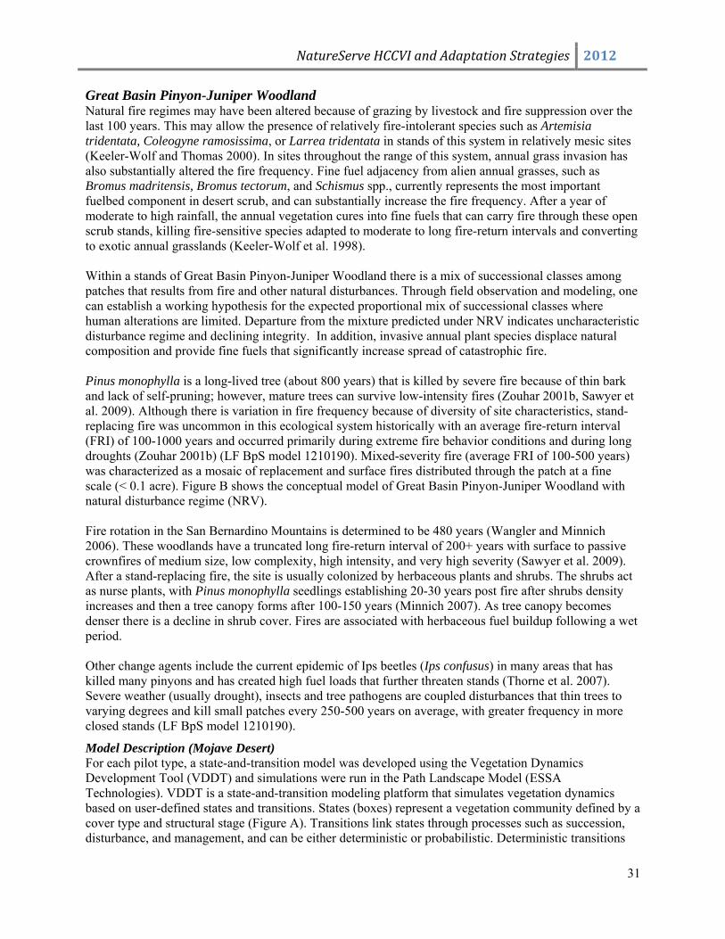
Great Basin Pinyon-Juniper Woodland Natural fire regimes may have been altered because of grazing by livestock and fire suppression over the last 100 years. This may allow the presence of relatively fire-intolerant species such as Artemisia tridentata, Coleogyne ramosissima, or Larrea tridentata in stands of this system in relatively mesic sites (Keeler-Wolf and Thomas 2000). In sites throughout the range of this system, annual grass invasion has also substantially altered the fire frequency. Fine fuel adjacency from alien annual grasses, such as Bromus madritensis, Bromus tectorum, and Schismus spp., currently represents the most important fuelbed component in desert scrub, and can substantially increase the fire frequency. After a year of moderate to high rainfall, the annual vegetation cures into fine fuels that can carry fire through these open scrub stands, killing fire-sensitive species adapted to moderate to long fire-return intervals and converting to exotic annual grasslands (Keeler-Wolf et al. 1998). Within a stands of Great Basin Pinyon-Juniper Woodland there is a mix of successional classes among patches that results from fire and other natural disturbances. Through field observation and modeling, one can establish a working hypothesis for the expected proportional mix of successional classes where human alterations are limited. Departure from the mixture predicted under NRV indicates uncharacteristic disturbance regime and declining integrity. In addition, invasive annual plant species displace natural composition and provide fine fuels that significantly increase spread of catastrophic fire. Pinus monophylla is a long-lived tree (about 800 years) that is killed by severe fire because of thin bark and lack of self-pruning; however, mature trees can survive low-intensity fires (Zouhar 2001b, Sawyer et al. 2009). Although there is variation in fire frequency because of diversity of site characteristics, stand-replacing fire was uncommon in this ecological system historically with an average fire-return interval (FRI) of 100-1000 years and occurred primarily during extreme fire behavior conditions and during long droughts (Zouhar 2001b) (LF BpS model 1210190). Mixed-severity fire (average FRI of 100-500 years) was characterized as a mosaic of replacement and surface fires distributed through the patch at a fine scale (< 0.1 acre). Figure B shows the conceptual model of Great Basin Pinyon-Juniper Woodland with natural disturbance regime (NRV). Fire rotation in the San Bernardino Mountains is determined to be 480 years (Wangler and Minnich 2006). These woodlands have a truncated long fire-return interval of 200+ years with surface to passive crownfires of medium size, low complexity, high intensity, and very high severity (Sawyer et al. 2009). After a stand-replacing fire, the site is usually colonized by herbaceous plants and shrubs. The shrubs act as nurse plants, with Pinus monophylla seedlings establishing 20-30 years post fire after shrubs density increases and then a tree canopy forms after 100-150 years (Minnich 2007). As tree canopy becomes denser there is a decline in shrub cover. Fires are associated with herbaceous fuel buildup following a wet period. Other change agents include the current epidemic of Ips beetles (Ips confusus) in many areas that has killed many pinyons and has created high fuel loads that further threaten stands (Thorne et al. 2007). Severe weather (usually drought), insects and tree pathogens are coupled disturbances that thin trees to varying degrees and kill small patches every 250-500 years on average, with greater frequency in more closed stands (LF BpS model 1210190).
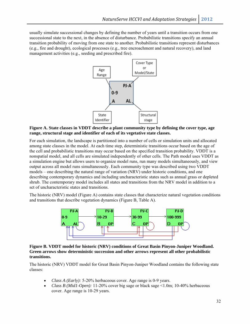
Model Description (Mojave Desert) For each pilot type, a state-and-transition model was developed using the Vegetation Dynamics Development Tool (VDDT) and simulations were run in the Path Landscape Model (ESSA Technologies). VDDT is a state-and-transition modeling platform that simulates vegetation dynamics based on user-defined states and transitions. States (boxes) represent a vegetation community defined by a cover type and structural stage (Figure A). Transitions link states through processes such as succession, disturbance, and management, and can be either deterministic or probabilistic. Deterministic transitions
NatureServe HCCVI and Adaptation Strategies 2012
32
usually simulate successional changes by defining the number of years until a transition occurs from one successional state to the next, in the absence of disturbance. Probabilistic transitions specify an annual transition probability of moving from one state to another. Probabilistic transitions represent disturbances (e.g., fire and drought), ecological processes (e.g., tree encroachment and natural recovery), and land management activities (e.g., seeding and prescribed fire).
Figure A. State classes in VDDT describe a plant community type by defining the cover type, age range, structural stage and identifier of each of its vegetative state classes.
For each simulation, the landscape is partitioned into a number of cells or simulation units and allocated among state classes in the model. At each time step, deterministic transitions occur based on the age of the cell and probabilistic transitions may occur based on the specified transition probability. VDDT is a nonspatial model, and all cells are simulated independently of other cells. The Path model uses VDDT as a simulation engine but allows users to organize model runs, run many models simultaneously, and view output across all model runs simultaneously. Each community type was described using two VDDT models – one describing the natural range of variation (NRV) under historic conditions, and one describing contemporary dynamics and including uncharacteristic states such as annual grass or depleted shrub. The contemporary model includes all states and transitions from the NRV model in addition to a set of uncharacteristic states and transitions.
The historic (NRV) model (Figure A) contains state classes that characterize natural vegetation conditions and transitions that describe vegetation dynamics (Figure B, Table A).
Figure B. VDDT model for historic (NRV) conditions of Great Basin Pinyon-Juniper Woodland. Green arrows show deterministic succession and other arrows represent all other probabilistic transitions.
The historic (NRV) VDDT model for Great Basin Pinyon-Juniper Woodland contains the following state classes:
• Class A (Early): 5-20% herbaceous cover. Age range is 0-9 years. • Class B (Mid1-Open): 11-20% cover big sage or black sage <1.0m; 10-40% herbaceous
cover. Age range is 10-29 years.
NatureServe HCCVI and Adaptation Strategies 2012
33
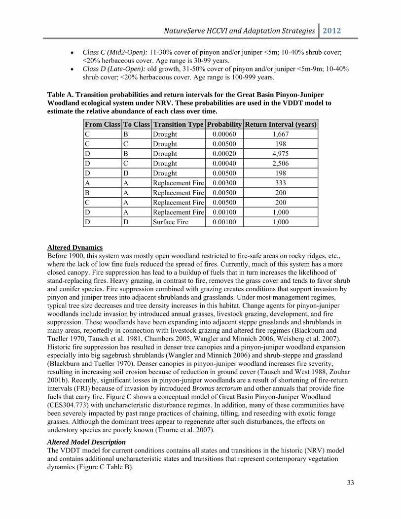
• Class C (Mid2-Open): 11-30% cover of pinyon and/or juniper <5m; 10-40% shrub cover; <20% herbaceous cover. Age range is 30-99 years.
• Class D (Late-Open): old growth, 31-50% cover of pinyon and/or juniper <5m-9m; 10-40% shrub cover; <20% herbaceous cover. Age range is 100-999 years.
Table A. Transition probabilities and return intervals for the Great Basin Pinyon-Juniper Woodland ecological system under NRV. These probabilities are used in the VDDT model to estimate the relative abundance of each class over time.
From Class To Class Transition Type Probability Return Interval (years) C B Drought 0.00060 1,667 C C Drought 0.00500 198 D B Drought 0.00020 4,975 D C Drought 0.00040 2,506 D D Drought 0.00500 198 A A Replacement Fire 0.00300 333 B A Replacement Fire 0.00500 200 C A Replacement Fire 0.00500 200 D A Replacement Fire 0.00100 1,000 D D Surface Fire 0.00100 1,000
Altered Dynamics Before 1900, this system was mostly open woodland restricted to fire-safe areas on rocky ridges, etc., where the lack of low fine fuels reduced the spread of fires. Currently, much of this system has a more closed canopy. Fire suppression has lead to a buildup of fuels that in turn increases the likelihood of stand-replacing fires. Heavy grazing, in contrast to fire, removes the grass cover and tends to favor shrub and conifer species. Fire suppression combined with grazing creates conditions that support invasion by pinyon and juniper trees into adjacent shrublands and grasslands. Under most management regimes, typical tree size decreases and tree density increases in this habitat. Change agents for pinyon-juniper woodlands include invasion by introduced annual grasses, livestock grazing, development, and fire suppression. These woodlands have been expanding into adjacent steppe grasslands and shrublands in many areas, reportedly in connection with livestock grazing and altered fire regimes (Blackburn and Tueller 1970, Tausch et al. 1981, Chambers 2005, Wangler and Minnich 2006, Weisberg et al. 2007). Historic fire suppression has resulted in denser tree canopies and a pinyon-juniper woodland expansion especially into big sagebrush shrublands (Wangler and Minnich 2006) and shrub-steppe and grassland (Blackburn and Tueller 1970). Denser canopies in pinyon-juniper woodland increases fire severity, resulting in increasing soil erosion because of reduction in ground cover (Tausch and West 1988, Zouhar 2001b). Recently, significant losses in pinyon-juniper woodlands are a result of shortening of fire-return intervals (FRI) because of invasion by introduced Bromus tectorum and other annuals that provide fine fuels that carry fire. Figure C shows a conceptual model of Great Basin Pinyon-Juniper Woodland (CES304.773) with uncharacteristic disturbance regimes. In addition, many of these communities have been severely impacted by past range practices of chaining, tilling, and reseeding with exotic forage grasses. Although the dominant trees appear to regenerate after such disturbances, the effects on understory species are poorly known (Thorne et al. 2007).
Altered Model Description The VDDT model for current conditions contains all states and transitions in the historic (NRV) model and contains additional uncharacteristic states and transitions that represent contemporary vegetation dynamics (Figure C Table B).
NatureServe HCCVI and Adaptation Strategies 2012
34
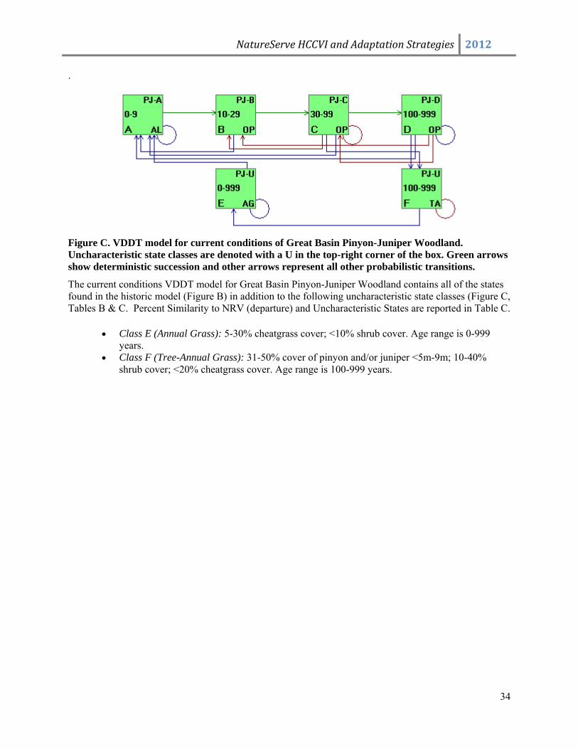
.
Figure C. VDDT model for current conditions of Great Basin Pinyon-Juniper Woodland. Uncharacteristic state classes are denoted with a U in the top-right corner of the box. Green arrows show deterministic succession and other arrows represent all other probabilistic transitions.
The current conditions VDDT model for Great Basin Pinyon-Juniper Woodland contains all of the states found in the historic model (Figure B) in addition to the following uncharacteristic state classes (Figure C, Tables B & C. Percent Similarity to NRV (departure) and Uncharacteristic States are reported in Table C.
• Class E (Annual Grass): 5-30% cheatgrass cover; <10% shrub cover. Age range is 0-999 years.
• Class F (Tree-Annual Grass): 31-50% cover of pinyon and/or juniper <5m-9m; 10-40% shrub cover; <20% cheatgrass cover. Age range is 100-999 years.
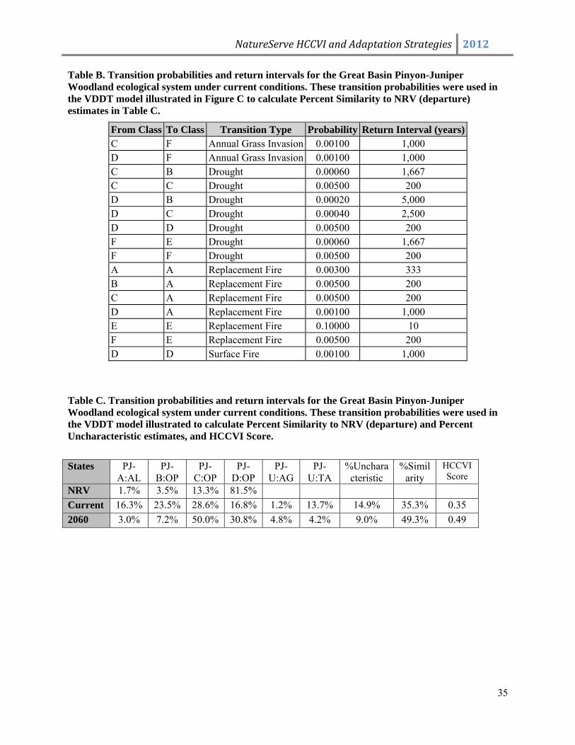
NatureServe HCCVI and Adaptation Strategies 2012
35
Table B. Transition probabilities and return intervals for the Great Basin Pinyon-Juniper Woodland ecological system under current conditions. These transition probabilities were used in the VDDT model illustrated in Figure C to calculate Percent Similarity to NRV (departure) estimates in Table C.
From Class To Class Transition Type Probability Return Interval (years)C F Annual Grass Invasion 0.00100 1,000 D F Annual Grass Invasion 0.00100 1,000 C B Drought 0.00060 1,667 C C Drought 0.00500 200 D B Drought 0.00020 5,000 D C Drought 0.00040 2,500 D D Drought 0.00500 200 F E Drought 0.00060 1,667 F F Drought 0.00500 200 A A Replacement Fire 0.00300 333 B A Replacement Fire 0.00500 200 C A Replacement Fire 0.00500 200 D A Replacement Fire 0.00100 1,000 E E Replacement Fire 0.10000 10 F E Replacement Fire 0.00500 200 D D Surface Fire 0.00100 1,000
Table C. Transition probabilities and return intervals for the Great Basin Pinyon-Juniper Woodland ecological system under current conditions. These transition probabilities were used in the VDDT model illustrated to calculate Percent Similarity to NRV (departure) and Percent Uncharacteristic estimates, and HCCVI Score.
States PJ-
A:AL PJ-
B:OP PJ-
C:OP PJ-
D:OP PJ-
U:AG PJ-
U:TA %Unchara
cteristic %Simil
arity HCCVI Score
NRV 1.7% 3.5% 13.3% 81.5% Current 16.3% 23.5% 28.6% 16.8% 1.2% 13.7% 14.9% 35.3% 0.35 2060 3.0% 7.2% 50.0% 30.8% 4.8% 4.2% 9.0% 49.3% 0.49
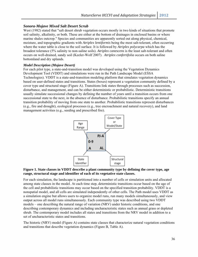
NatureServe HCCVI and Adaptation Strategies 2012
36
Sonora-Mojave Mixed Salt Desert Scrub West (1982) stated that "salt desert shrub vegetation occurs mostly in two kinds of situations that promote soil salinity, alkalinity, or both. These are either at the bottom of drainages in enclosed basins or where marine shales outcrop." Species and communities are apparently sorted out along physical, chemical, moisture, and topographic gradients with Atriplex lentiformis being the most salt-tolerant, often occurring where the water table is close to the soil surface. It is followed by Atriplex polycarpa which has the broadest tolerance (5% salinity to non-saline soils). Atriplex canescens is the least salt-tolerant and often occurs on well-drained, sandy soil (Keeler-Wolf 2007). Atriplex confertifolia occurs on both saline bottomland and dry uplands.
Model Description (Mojave Desert) For each pilot type, a state-and-transition model was developed using the Vegetation Dynamics Development Tool (VDDT) and simulations were run in the Path Landscape Model (ESSA Technologies). VDDT is a state-and-transition modeling platform that simulates vegetation dynamics based on user-defined states and transitions. States (boxes) represent a vegetation community defined by a cover type and structural stage (Figure A). Transitions link states through processes such as succession, disturbance, and management, and can be either deterministic or probabilistic. Deterministic transitions usually simulate successional changes by defining the number of years until a transition occurs from one successional state to the next, in the absence of disturbance. Probabilistic transitions specify an annual transition probability of moving from one state to another. Probabilistic transitions represent disturbances (e.g., fire and drought), ecological processes (e.g., tree encroachment and natural recovery), and land management activities (e.g., seeding and prescribed fire).
Figure 1. State classes in VDDT describe a plant community type by defining the cover type, age range, structural stage and identifier of each of its vegetative state classes.
For each simulation, the landscape is partitioned into a number of cells or simulation units and allocated among state classes in the model. At each time step, deterministic transitions occur based on the age of the cell and probabilistic transitions may occur based on the specified transition probability. VDDT is a nonspatial model, and all cells are simulated independently of other cells. The Path model uses VDDT as a simulation engine but allows users to organize model runs, run many models simultaneously, and view output across all model runs simultaneously. Each community type was described using two VDDT models – one describing the natural range of variation (NRV) under historic conditions, and one describing contemporary dynamics and including uncharacteristic states such as annual grass or depleted shrub. The contemporary model includes all states and transitions from the NRV model in addition to a set of uncharacteristic states and transitions.
The historic (NRV) model (Figure A) contains state classes that characterize natural vegetation conditions and transitions that describe vegetation dynamics (Figure B, Table A).
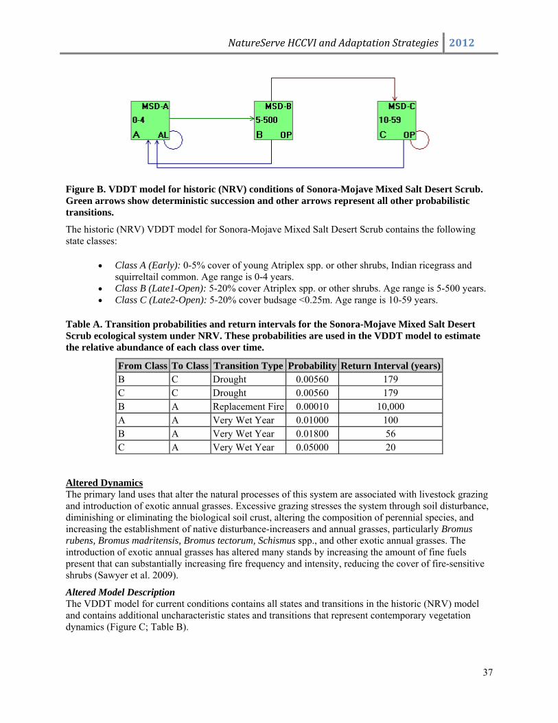
NatureServe HCCVI and Adaptation Strategies 2012
37
Figure B. VDDT model for historic (NRV) conditions of Sonora-Mojave Mixed Salt Desert Scrub. Green arrows show deterministic succession and other arrows represent all other probabilistic transitions.
The historic (NRV) VDDT model for Sonora-Mojave Mixed Salt Desert Scrub contains the following state classes:
• Class A (Early): 0-5% cover of young Atriplex spp. or other shrubs, Indian ricegrass and squirreltail common. Age range is 0-4 years.
• Class B (Late1-Open): 5-20% cover Atriplex spp. or other shrubs. Age range is 5-500 years. • Class C (Late2-Open): 5-20% cover budsage <0.25m. Age range is 10-59 years.
Table A. Transition probabilities and return intervals for the Sonora-Mojave Mixed Salt Desert Scrub ecological system under NRV. These probabilities are used in the VDDT model to estimate the relative abundance of each class over time.
From Class To Class Transition Type Probability Return Interval (years) B C Drought 0.00560 179 C C Drought 0.00560 179 B A Replacement Fire 0.00010 10,000 A A Very Wet Year 0.01000 100 B A Very Wet Year 0.01800 56 C A Very Wet Year 0.05000 20
Altered Dynamics The primary land uses that alter the natural processes of this system are associated with livestock grazing and introduction of exotic annual grasses. Excessive grazing stresses the system through soil disturbance, diminishing or eliminating the biological soil crust, altering the composition of perennial species, and increasing the establishment of native disturbance-increasers and annual grasses, particularly Bromus rubens, Bromus madritensis, Bromus tectorum, Schismus spp., and other exotic annual grasses. The introduction of exotic annual grasses has altered many stands by increasing the amount of fine fuels present that can substantially increasing fire frequency and intensity, reducing the cover of fire-sensitive shrubs (Sawyer et al. 2009).
Altered Model Description The VDDT model for current conditions contains all states and transitions in the historic (NRV) model and contains additional uncharacteristic states and transitions that represent contemporary vegetation dynamics (Figure C; Table B).
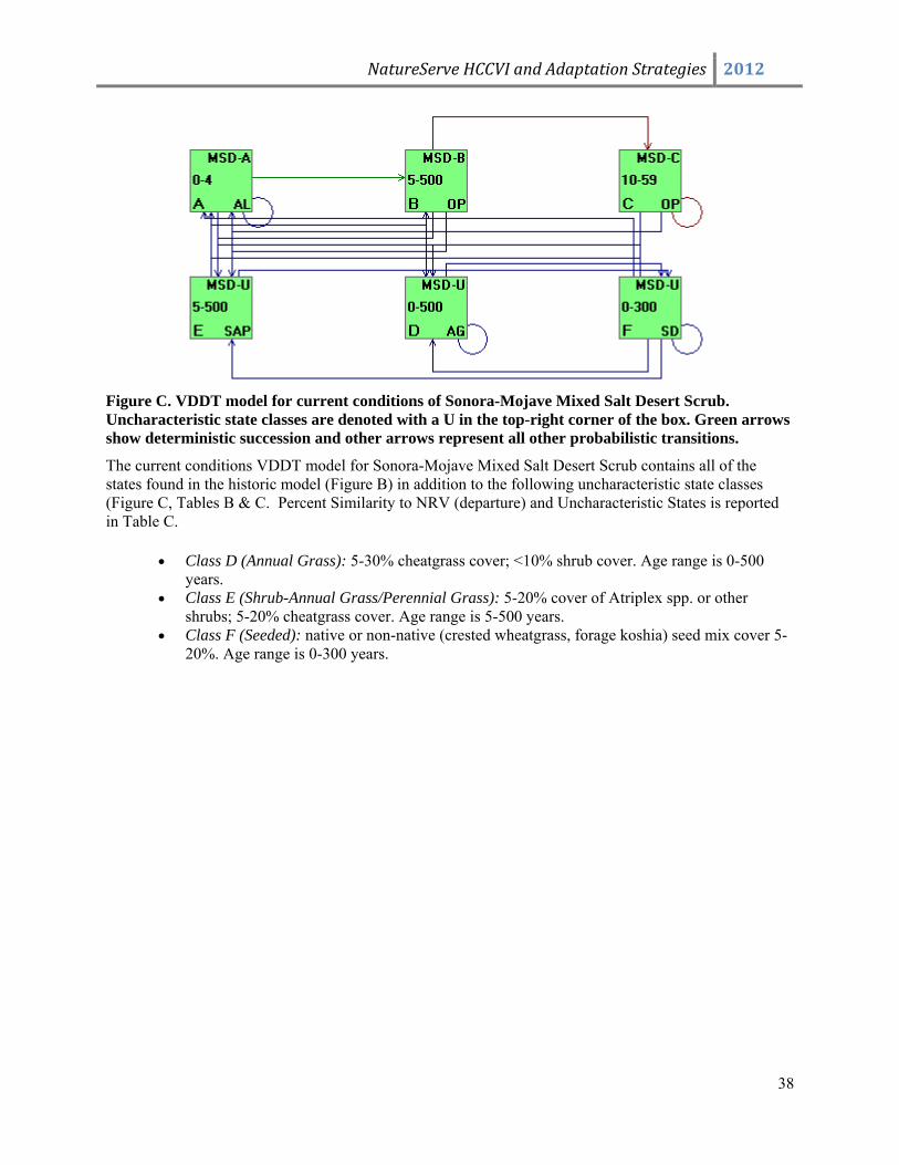
NatureServe HCCVI and Adaptation Strategies 2012
38
Figure C. VDDT model for current conditions of Sonora-Mojave Mixed Salt Desert Scrub. Uncharacteristic state classes are denoted with a U in the top-right corner of the box. Green arrows show deterministic succession and other arrows represent all other probabilistic transitions.
The current conditions VDDT model for Sonora-Mojave Mixed Salt Desert Scrub contains all of the states found in the historic model (Figure B) in addition to the following uncharacteristic state classes (Figure C, Tables B & C. Percent Similarity to NRV (departure) and Uncharacteristic States is reported in Table C.
• Class D (Annual Grass): 5-30% cheatgrass cover; <10% shrub cover. Age range is 0-500 years.
• Class E (Shrub-Annual Grass/Perennial Grass): 5-20% cover of Atriplex spp. or other shrubs; 5-20% cheatgrass cover. Age range is 5-500 years.
• Class F (Seeded): native or non-native (crested wheatgrass, forage koshia) seed mix cover 5-20%. Age range is 0-300 years.
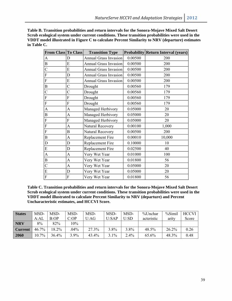
NatureServe HCCVI and Adaptation Strategies 2012
39
Table B. Transition probabilities and return intervals for the Sonora-Mojave Mixed Salt Desert Scrub ecological system under current conditions. These transition probabilities were used in the VDDT model illustrated in Figure C to calculate Percent Similarity to NRV (departure) estimates in Table C.
From Class To Class Transition Type Probability Return Interval (years)A D Annual Grass Invasion 0.00500 200 B E Annual Grass Invasion 0.00500 200 C E Annual Grass Invasion 0.00500 200 F D Annual Grass Invasion 0.00500 200 F E Annual Grass Invasion 0.00500 200 B C Drought 0.00560 179 C C Drought 0.00560 179 F F Drought 0.00560 179 F F Drought 0.00560 179 A A Managed Herbivory 0.05000 20 B A Managed Herbivory 0.05000 20 F F Managed Herbivory 0.05000 20 F A Natural Recovery 0.00100 1,000 F B Natural Recovery 0.00500 200 B A Replacement Fire 0.00010 10,000 D D Replacement Fire 0.10000 10 E D Replacement Fire 0.02500 40 A A Very Wet Year 0.01000 100 B A Very Wet Year 0.01800 56 C A Very Wet Year 0.05000 20 E D Very Wet Year 0.05000 20 F F Very Wet Year 0.01800 56
Table C. Transition probabilities and return intervals for the Sonora-Mojave Mixed Salt Desert Scrub ecological system under current conditions. These transition probabilities were used in the VDDT model illustrated to calculate Percent Similarity to NRV (departure) and Percent Uncharacteristic estimates, and HCCVI Score.
States MSD-
A:AL MSD-B:OP
MSD-C:OP
MSD-U:AG
MSD-U:SAP
MSD-U:SD
%Unchar acteristic
%Simil arity
HCCVI Score
NRV 8% 82% 10% Current 46.7% 18.2% .04% 27.3% 3.8% 3.8% 48.5% 26.2% 0.26 2060 10.7% 36.4% 3.9% 43.4% 3.1% 2.4% 65.6% 48.3% 0.48
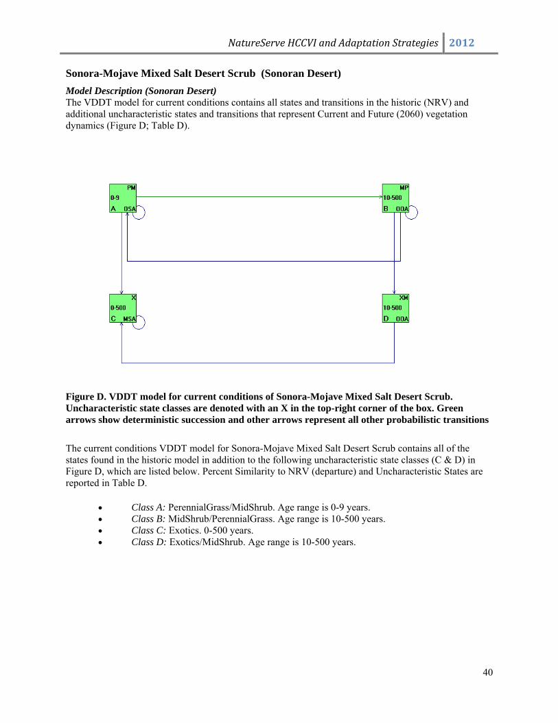
NatureServe HCCVI and Adaptation Strategies 2012
40
Sonora-Mojave Mixed Salt Desert Scrub (Sonoran Desert) Model Description (Sonoran Desert) The VDDT model for current conditions contains all states and transitions in the historic (NRV) and additional uncharacteristic states and transitions that represent Current and Future (2060) vegetation dynamics (Figure D; Table D).
Figure D. VDDT model for current conditions of Sonora-Mojave Mixed Salt Desert Scrub. Uncharacteristic state classes are denoted with an X in the top-right corner of the box. Green arrows show deterministic succession and other arrows represent all other probabilistic transitions
The current conditions VDDT model for Sonora-Mojave Mixed Salt Desert Scrub contains all of the states found in the historic model in addition to the following uncharacteristic state classes (C & D) in Figure D, which are listed below. Percent Similarity to NRV (departure) and Uncharacteristic States are reported in Table D.
• Class A: PerennialGrass/MidShrub. Age range is 0-9 years. • Class B: MidShrub/PerennialGrass. Age range is 10-500 years. • Class C: Exotics. 0-500 years. • Class D: Exotics/MidShrub. Age range is 10-500 years.
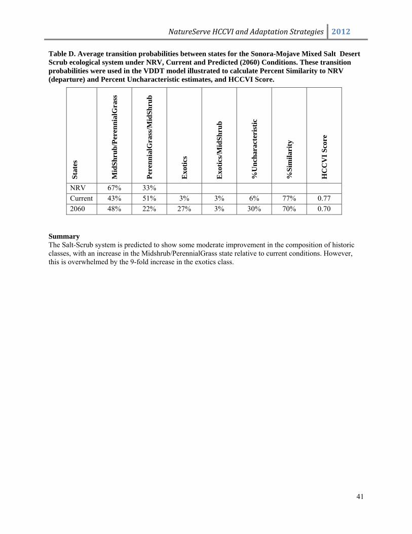
NatureServe HCCVI and Adaptation Strategies 2012
41
Table D. Average transition probabilities between states for the Sonora-Mojave Mixed Salt Desert Scrub ecological system under NRV, Current and Predicted (2060) Conditions. These transition probabilities were used in the VDDT model illustrated to calculate Percent Similarity to NRV (departure) and Percent Uncharacteristic estimates, and HCCVI Score.
Stat
es
Mid
Shru
b/Pe
renn
ialG
rass
Pere
nnia
lGra
ss/M
idSh
rub
Exo
tics
Exo
tics/
Mid
Shru
b
%U
ncha
ract
eris
tic
%Si
mila
rity
HC
CV
I Sco
re
NRV 67% 33% Current 43% 51% 3% 3% 6% 77% 0.77 2060 48% 22% 27% 3% 30% 70% 0.70
Summary The Salt-Scrub system is predicted to show some moderate improvement in the composition of historic classes, with an increase in the Midshrub/PerennialGrass state relative to current conditions. However, this is overwhelmed by the 9-fold increase in the exotics class.
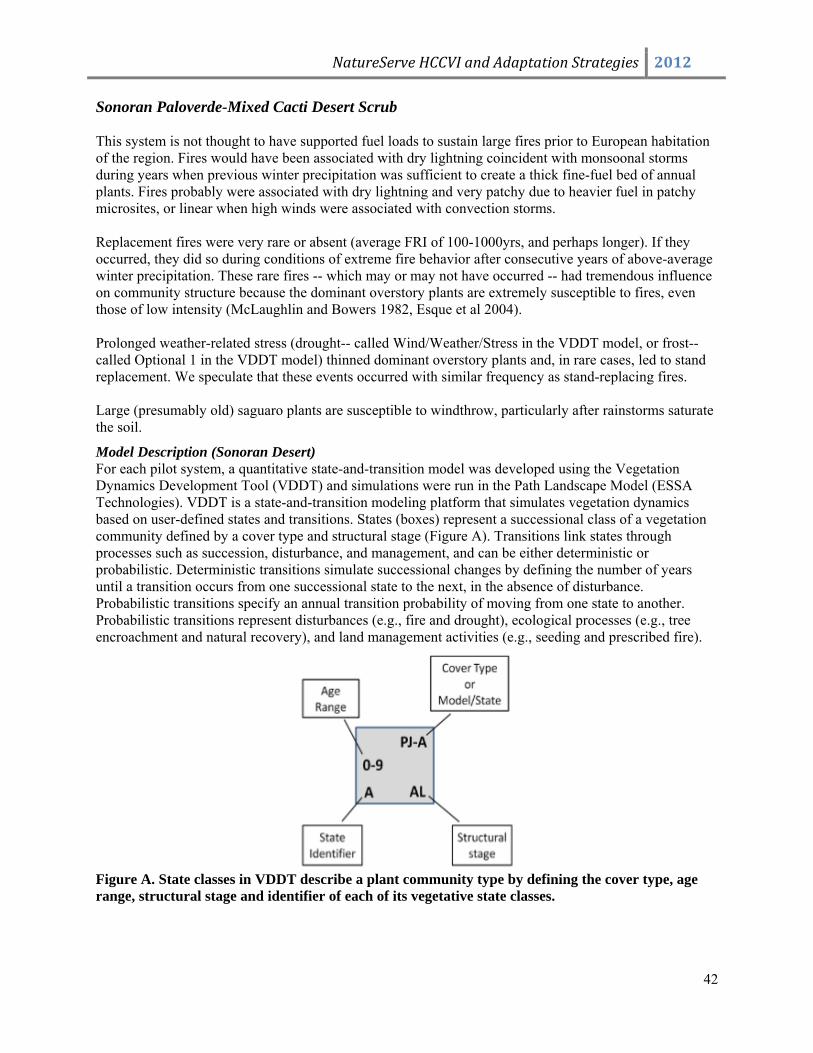
NatureServe HCCVI and Adaptation Strategies 2012
42
Sonoran Paloverde-Mixed Cacti Desert Scrub This system is not thought to have supported fuel loads to sustain large fires prior to European habitation of the region. Fires would have been associated with dry lightning coincident with monsoonal storms during years when previous winter precipitation was sufficient to create a thick fine-fuel bed of annual plants. Fires probably were associated with dry lightning and very patchy due to heavier fuel in patchy microsites, or linear when high winds were associated with convection storms. Replacement fires were very rare or absent (average FRI of 100-1000yrs, and perhaps longer). If they occurred, they did so during conditions of extreme fire behavior after consecutive years of above-average winter precipitation. These rare fires -- which may or may not have occurred -- had tremendous influence on community structure because the dominant overstory plants are extremely susceptible to fires, even those of low intensity (McLaughlin and Bowers 1982, Esque et al 2004). Prolonged weather-related stress (drought-- called Wind/Weather/Stress in the VDDT model, or frost-- called Optional 1 in the VDDT model) thinned dominant overstory plants and, in rare cases, led to stand replacement. We speculate that these events occurred with similar frequency as stand-replacing fires. Large (presumably old) saguaro plants are susceptible to windthrow, particularly after rainstorms saturate the soil.
Model Description (Sonoran Desert) For each pilot system, a quantitative state-and-transition model was developed using the Vegetation Dynamics Development Tool (VDDT) and simulations were run in the Path Landscape Model (ESSA Technologies). VDDT is a state-and-transition modeling platform that simulates vegetation dynamics based on user-defined states and transitions. States (boxes) represent a successional class of a vegetation community defined by a cover type and structural stage (Figure A). Transitions link states through processes such as succession, disturbance, and management, and can be either deterministic or probabilistic. Deterministic transitions simulate successional changes by defining the number of years until a transition occurs from one successional state to the next, in the absence of disturbance. Probabilistic transitions specify an annual transition probability of moving from one state to another. Probabilistic transitions represent disturbances (e.g., fire and drought), ecological processes (e.g., tree encroachment and natural recovery), and land management activities (e.g., seeding and prescribed fire).
Figure A. State classes in VDDT describe a plant community type by defining the cover type, age range, structural stage and identifier of each of its vegetative state classes.
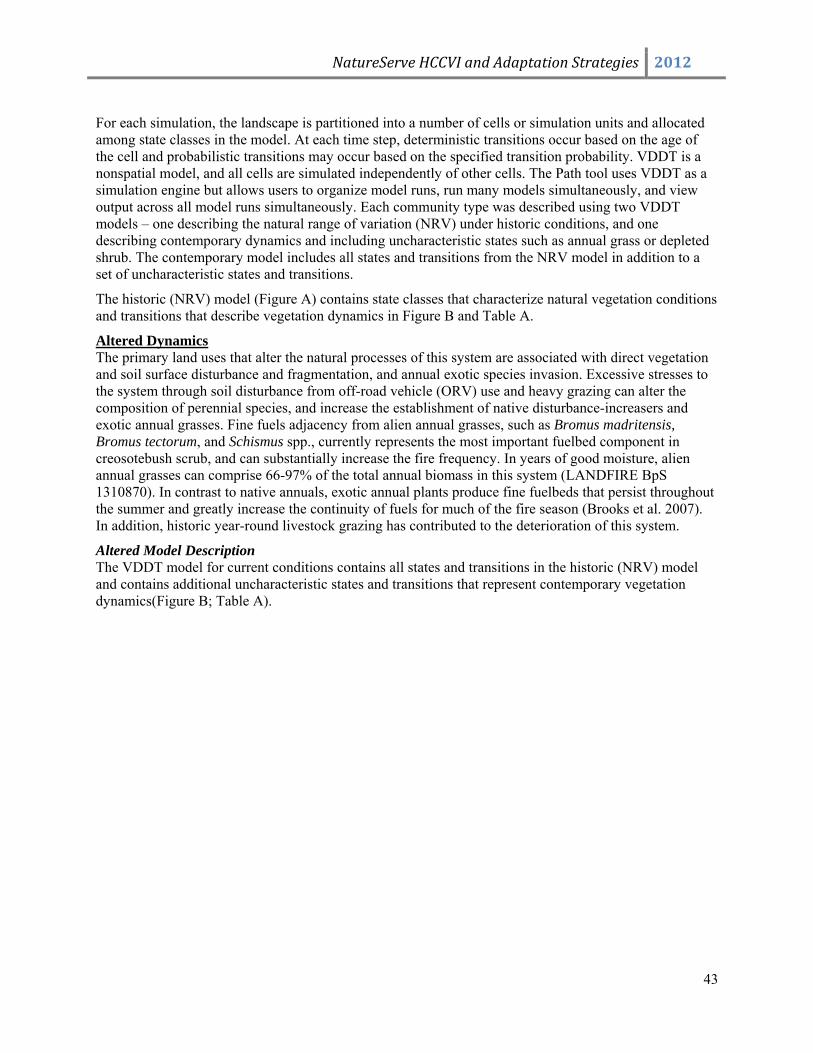
NatureServe HCCVI and Adaptation Strategies 2012
43
For each simulation, the landscape is partitioned into a number of cells or simulation units and allocated among state classes in the model. At each time step, deterministic transitions occur based on the age of the cell and probabilistic transitions may occur based on the specified transition probability. VDDT is a nonspatial model, and all cells are simulated independently of other cells. The Path tool uses VDDT as a simulation engine but allows users to organize model runs, run many models simultaneously, and view output across all model runs simultaneously. Each community type was described using two VDDT models – one describing the natural range of variation (NRV) under historic conditions, and one describing contemporary dynamics and including uncharacteristic states such as annual grass or depleted shrub. The contemporary model includes all states and transitions from the NRV model in addition to a set of uncharacteristic states and transitions.
The historic (NRV) model (Figure A) contains state classes that characterize natural vegetation conditions and transitions that describe vegetation dynamics in Figure B and Table A.
Altered Dynamics The primary land uses that alter the natural processes of this system are associated with direct vegetation and soil surface disturbance and fragmentation, and annual exotic species invasion. Excessive stresses to the system through soil disturbance from off-road vehicle (ORV) use and heavy grazing can alter the composition of perennial species, and increase the establishment of native disturbance-increasers and exotic annual grasses. Fine fuels adjacency from alien annual grasses, such as Bromus madritensis, Bromus tectorum, and Schismus spp., currently represents the most important fuelbed component in creosotebush scrub, and can substantially increase the fire frequency. In years of good moisture, alien annual grasses can comprise 66-97% of the total annual biomass in this system (LANDFIRE BpS 1310870). In contrast to native annuals, exotic annual plants produce fine fuelbeds that persist throughout the summer and greatly increase the continuity of fuels for much of the fire season (Brooks et al. 2007). In addition, historic year-round livestock grazing has contributed to the deterioration of this system.
Altered Model Description The VDDT model for current conditions contains all states and transitions in the historic (NRV) model and contains additional uncharacteristic states and transitions that represent contemporary vegetation dynamics(Figure B; Table A).
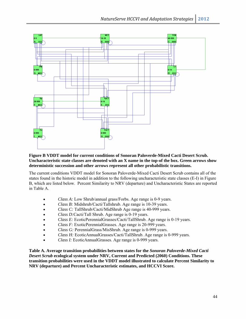
NatureServe HCCVI and Adaptation Strategies 2012
44
Figure B VDDT model for current conditions of Sonoran Paloverde-Mixed Cacti Desert Scrub. Uncharacteristic state classes are denoted with an X name in the top-of the box. Green arrows show deterministic succession and other arrows represent all other probabilistic transitions.
The current conditions VDDT model for Sonoran Paloverde-Mixed Cacti Desert Scrub contains all of the states found in the historic model in addition to the following uncharacteristic state classes (E-I) in Figure B, which are listed below. Percent Similarity to NRV (departure) and Uncharacteristic States are reported in Table A.
• Class A: Low Shrub/annual grass/Forbs. Age range is 0-9 years. • Class B: Midshrub/Cacti/Tallshrub. Age range is 10-39 years. • Class C: TallShrub/Cacti/MidShrub Age range is 40-999 years. • Class D:Cacti/Tall Shrub. Age range is 0-19 years. • Class E: EcoticPerennialGrasses/Cacti/TallShrub. Age range is 0-19 years. • Class F: ExoticPerennialGrasses. Age range is 20-999 years. • Class G: PerennialGrass/MisShrub. Age range is 0-999 years. • Class H: EcoticAnnualGrasses/Cacti/TallShrub. Age range is 0-999 years. • Class I: EcoticAnnualGrasses. Age range is 0-999 years.
Table A. Average transition probabilities between states for the Sonoran Paloverde-Mixed Cacti Desert Scrub ecological system under NRV, Current and Predicted (2060) Conditions. These transition probabilities were used in the VDDT model illustrated to calculate Percent Similarity to NRV (departure) and Percent Uncharacteristic estimates, and HCCVI Score.
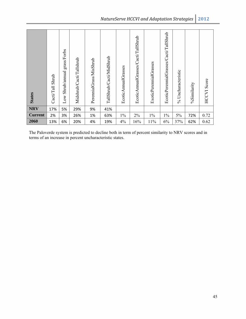
NatureServe HCCVI and Adaptation Strategies 2012
45
Stat
es
Cac
ti/Ta
ll Sh
rub
Low
Shr
ub/a
nnua
l gra
ss/F
orbs
Mid
shru
b/C
acti/
Talls
hrub
Pere
nnia
lGra
ss/M
isSh
rub
TallS
hrub
/Cac
ti/M
idSh
rub
Ecot
icA
nnua
lGra
sses
Ecot
icA
nnua
lGra
sses
/Cac
ti/Ta
llShr
ub
Exot
icPe
renn
ialG
rass
es
Ecot
icPe
renn
ialG
rass
es/C
acti/
TallS
hrub
% U
ncha
ract
eris
tic
%Si
mila
rity
HC
CV
I Sco
re
NRV 17% 5% 29% 9% 41% Current 2% 3% 26% 1% 63% 1% 2% 1% 1% 5% 72% 0.72 2060 13% 6% 20% 4% 19% 4% 16% 11% 6% 37% 62% 0.62 The Paloverde system is predicted to decline both in term of percent similarity to NRV scores and in terms of an increase in percent uncharacteristic states.
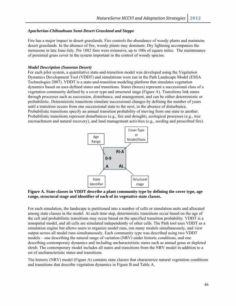
NatureServe HCCVI and Adaptation Strategies 2012
46
Apacherian-Chihuahuan Semi-Desert Grassland and Steppe Fire has a major impact in desert grasslands. Fire controls the abundance of woody plants and maintains desert grasslands. In the absence of fire, woody plants may dominate. Dry lightning accompanies the monsoons in late June-July. Pre 1882 fires were extensive, up to 100s of square miles. The maintenance of perennial grass cover in the system important in the control of woody species.
Model Description (Sonoran Desert) For each pilot system, a quantitative state-and-transition model was developed using the Vegetation Dynamics Development Tool (VDDT) and simulations were run in the Path Landscape Model (ESSA Technologies 2007). VDDT is a state-and-transition modeling platform that simulates vegetation dynamics based on user-defined states and transitions. States (boxes) represent a successional class of a vegetation community defined by a cover type and structural stage (Figure A). Transitions link states through processes such as succession, disturbance, and management, and can be either deterministic or probabilistic. Deterministic transitions simulate successional changes by defining the number of years until a transition occurs from one successional state to the next, in the absence of disturbance. Probabilistic transitions specify an annual transition probability of moving from one state to another. Probabilistic transitions represent disturbances (e.g., fire and drought), ecological processes (e.g., tree encroachment and natural recovery), and land management activities (e.g., seeding and prescribed fire).
Figure A. State classes in VDDT describe a plant community type by defining the cover type, age range, structural stage and identifier of each of its vegetative state classes.
For each simulation, the landscape is partitioned into a number of cells or simulation units and allocated among state classes in the model. At each time step, deterministic transitions occur based on the age of the cell and probabilistic transitions may occur based on the specified transition probability. VDDT is a nonspatial model, and all cells are simulated independently of other cells. The Path tool uses VDDT as a simulation engine but allows users to organize model runs, run many models simultaneously, and view output across all model runs simultaneously. Each community type was described using two VDDT models – one describing the natural range of variation (NRV) under historic conditions, and one describing contemporary dynamics and including uncharacteristic states such as annual grass or depleted shrub. The contemporary model includes all states and transitions from the NRV model in addition to a set of uncharacteristic states and transitions.
The historic (NRV) model (Figure A) contains state classes that characterize natural vegetation conditions and transitions that describe vegetation dynamics in Figure B and Table A.
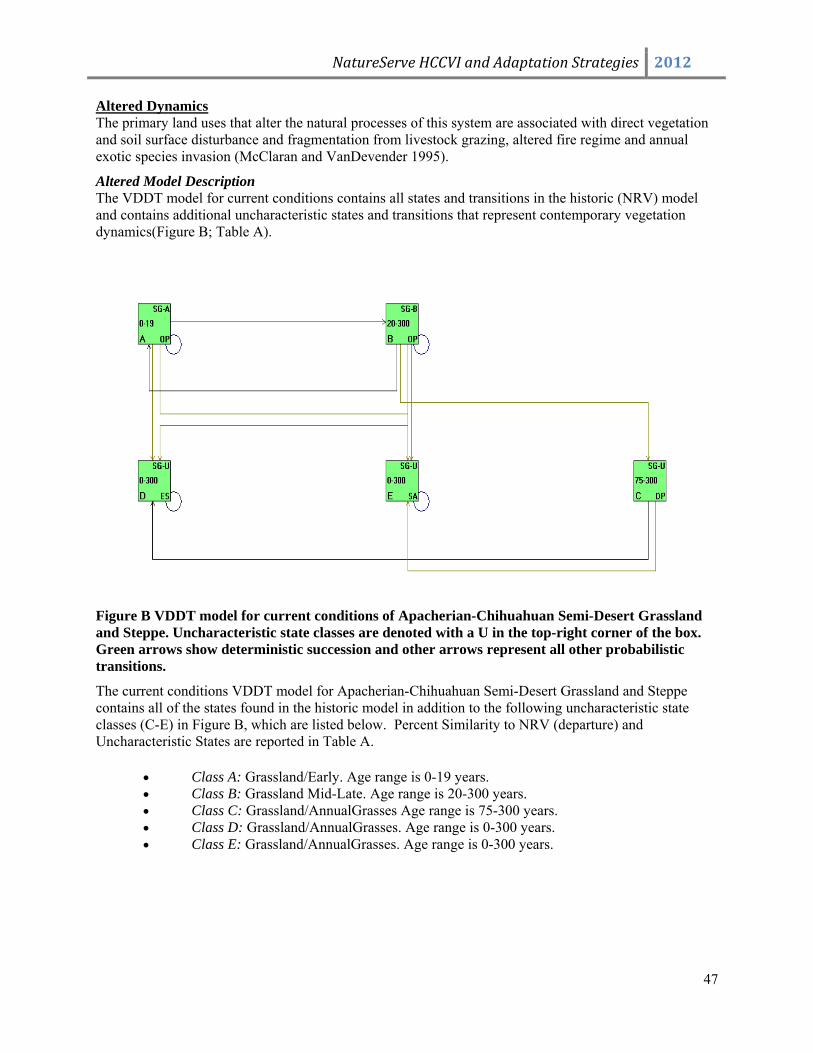
NatureServe HCCVI and Adaptation Strategies 2012
47
Altered Dynamics The primary land uses that alter the natural processes of this system are associated with direct vegetation and soil surface disturbance and fragmentation from livestock grazing, altered fire regime and annual exotic species invasion (McClaran and VanDevender 1995).
Altered Model Description The VDDT model for current conditions contains all states and transitions in the historic (NRV) model and contains additional uncharacteristic states and transitions that represent contemporary vegetation dynamics(Figure B; Table A).
Figure B VDDT model for current conditions of Apacherian-Chihuahuan Semi-Desert Grassland and Steppe. Uncharacteristic state classes are denoted with a U in the top-right corner of the box. Green arrows show deterministic succession and other arrows represent all other probabilistic transitions.
The current conditions VDDT model for Apacherian-Chihuahuan Semi-Desert Grassland and Steppe contains all of the states found in the historic model in addition to the following uncharacteristic state classes (C-E) in Figure B, which are listed below. Percent Similarity to NRV (departure) and Uncharacteristic States are reported in Table A.
• Class A: Grassland/Early. Age range is 0-19 years. • Class B: Grassland Mid-Late. Age range is 20-300 years. • Class C: Grassland/AnnualGrasses Age range is 75-300 years. • Class D: Grassland/AnnualGrasses. Age range is 0-300 years. • Class E: Grassland/AnnualGrasses. Age range is 0-300 years.
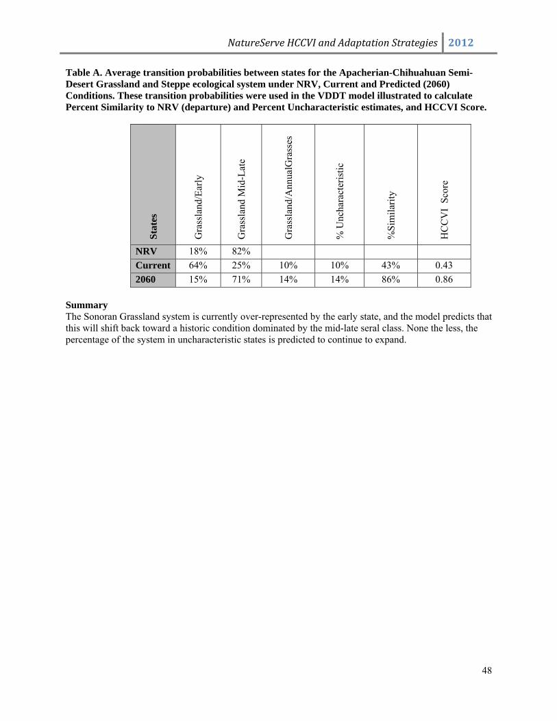
NatureServe HCCVI and Adaptation Strategies 2012
48
Table A. Average transition probabilities between states for the Apacherian-Chihuahuan Semi-Desert Grassland and Steppe ecological system under NRV, Current and Predicted (2060) Conditions. These transition probabilities were used in the VDDT model illustrated to calculate Percent Similarity to NRV (departure) and Percent Uncharacteristic estimates, and HCCVI Score.
Stat
es
Gra
ssla
nd/E
arly
Gra
ssla
nd M
id-L
ate
Gra
ssla
nd/A
nnua
lGra
sses
% U
ncha
ract
eris
tic
%Si
mila
rity
HC
CV
I Sc
ore
NRV 18% 82% Current 64% 25% 10% 10% 43% 0.43 2060 15% 71% 14% 14% 86% 0.86
Summary The Sonoran Grassland system is currently over-represented by the early state, and the model predicts that this will shift back toward a historic condition dominated by the mid-late seral class. None the less, the percentage of the system in uncharacteristic states is predicted to continue to expand.
NatureServe HCCVI and Adaptation Strategies 2012
49
INDIRECT EFFECTS Indirect effects include estimates of past, current ecosystem integrity and their potential interacting effects of climate change. Ecological conditions and landscape dynamics that support ecological systems or species habitat are affected by land use. So for example, these measures address the degree of landscape fragmentation or other anthropogenic impacts (such as invasive species) in the landscapes supporting a given community type. Land use impacts vary in their intensity where they occur, as well as their ecological effects with distance from source. While producing actual maps of historical fragmentation during the early-mid 20th century is quite challenging and often impossible, a qualitative estimate can often be feasible, based on the estimated extent of roads and other anthropogenic disturbances. Land and water use effects measures were developed for each community type for the past (1960) and current (2010) time periods.
Relative Landscape Condition Ecological condition commonly refers to the state of the physical, chemical, and biological characteristics of natural ecosystems, and their interacting processes. Many human land uses affect ecological condition, (e.g., through vegetation removal or alteration, stream diversion or altered natural hydrology, introduction of non-native and invasive species, etc.). Landscape condition assessments commonly apply principles of landscape ecology with mapped information to characterize ecological condition for a given area (e.g., USEPA 2001, Sanderson et al. 2002). Since human land uses - such as built infrastructure for transportation or urban/industry, and land cover such as for agriculture or other vegetation alteration – are increasingly available in mapped form, they can be used to spatially model inferences about ecological stress and ecological condition. Maps of this nature can be particularly helpful for identifying relatively unaltered landscape blocks, or for making inferences about the relative ecological integrity of natural habitats on the ground. They can also be used for screening ecological reference sites; i.e., a set of sites where anthropogenic stressors range from low to high. Ecological condition within reference sites is often further characterized in the field to determine how ecological processes respond to specific stressors, but spatial models can provide a very powerful starting point to build upon (Faber-Langendoen et al. 2006, 2012). Knowledge from reference sites may then apply to surroundings for many types of environmental decisions. The Landscape Condition Models used in this project build on a growing body of published methods and software tools for ecological effects assessment and spatial modeling; all aiming to characterize relative ecological condition of landscapes (e.g., Knick and Rotenberry 1995, Forman and Alexander 1998, Trombulak and Frissel 1999, Theobald 2001, Seiler 2001, Sanderson et al. 2002, Riitters and Wickham 2003, Brown and Vivas 2005, Hansen et al. 2005, Leu et al. 2008, Comer and Hak 2009, Comer and Hak in prep, Theobald 2010, Rocchio and Crawford 2011). The intent of this modeling approach is to use regionally available spatial data to transparently express user knowledge regarding the relative effects of land uses on natural ecosystems and habitats. In these cases, the authors’ expert knowledge forms the basis of stressor selection, and relative weightings, but numerous examples from published literature have been drawn upon to parameterize the model for application in this ecoregion. Independent data sets were drawn upon for subsequent model evaluation. The current model applied to the Mojave Desert has been developed and evaluated for the entire western United States, and then customized for use within the ecoregion. Western regional model development and evaluation was completed in cooperation with the Western Governors Association landscape connectivity working group (J. Pierce pers. comm. 2012). A similar model was developed to cover Mexican portions of the Sonoran Desert. Each input data layer is summarized to a 90m grid and, where the land use occurs, given a site impact score from 0.05 to 0.9 (Table A2-2) reflecting presumed ecological stress or impact. Values close to 1.0
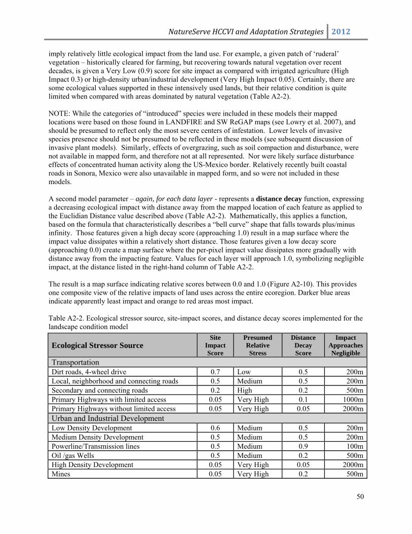
NatureServe HCCVI and Adaptation Strategies 2012
50
imply relatively little ecological impact from the land use. For example, a given patch of ‘ruderal’ vegetation – historically cleared for farming, but recovering towards natural vegetation over recent decades, is given a Very Low (0.9) score for site impact as compared with irrigated agriculture (High Impact 0.3) or high-density urban/industrial development (Very High Impact 0.05). Certainly, there are some ecological values supported in these intensively used lands, but their relative condition is quite limited when compared with areas dominated by natural vegetation (Table A2-2). NOTE: While the categories of “introduced” species were included in these models their mapped locations were based on those found in LANDFIRE and SW ReGAP maps (see Lowry et al. 2007), and should be presumed to reflect only the most severe centers of infestation. Lower levels of invasive species presence should not be presumed to be reflected in these models (see subsequent discussion of invasive plant models). Similarly, effects of overgrazing, such as soil compaction and disturbance, were not available in mapped form, and therefore not at all represented. Nor were likely surface disturbance effects of concentrated human activity along the US-Mexico border. Relatively recently built coastal roads in Sonora, Mexico were also unavailable in mapped form, and so were not included in these models. A second model parameter – again, for each data layer - represents a distance decay function, expressing a decreasing ecological impact with distance away from the mapped location of each feature as applied to the Euclidian Distance value described above (Table A2-2). Mathematically, this applies a function, based on the formula that characteristically describes a “bell curve” shape that falls towards plus/minus infinity. Those features given a high decay score (approaching 1.0) result in a map surface where the impact value dissipates within a relatively short distance. Those features given a low decay score (approaching 0.0) create a map surface where the per-pixel impact value dissipates more gradually with distance away from the impacting feature. Values for each layer will approach 1.0, symbolizing negligible impact, at the distance listed in the right-hand column of Table A2-2. The result is a map surface indicating relative scores between 0.0 and 1.0 (Figure A2-10). This provides one composite view of the relative impacts of land uses across the entire ecoregion. Darker blue areas indicate apparently least impact and orange to red areas most impact. Table A2-2. Ecological stressor source, site-impact scores, and distance decay scores implemented for the landscape condition model
Ecological Stressor Source Site
Impact Score
Presumed Relative Stress
Distance Decay Score
Impact Approaches Negligible
Transportation Dirt roads, 4-wheel drive 0.7 Low 0.5 200mLocal, neighborhood and connecting roads 0.5 Medium 0.5 200mSecondary and connecting roads 0.2 High 0.2 500mPrimary Highways with limited access 0.05 Very High 0.1 1000mPrimary Highways without limited access 0.05 Very High 0.05 2000mUrban and Industrial Development Low Density Development 0.6 Medium 0.5 200mMedium Density Development 0.5 Medium 0.5 200mPowerline/Transmission lines 0.5 Medium 0.9 100mOil /gas Wells 0.5 Medium 0.2 500mHigh Density Development 0.05 Very High 0.05 2000mMines 0.05 Very High 0.2 500m
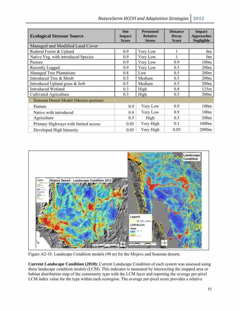
NatureServe HCCVI and Adaptation Strategies 2012
51
Ecological Stressor Source Site
Impact Score
Presumed Relative Stress
Distance Impact Decay Approaches Score Negligible
Managed and Modified Land Cover Ruderal Forest & Upland 0.9 Very Low 1 0mNative Veg. with introduced Species 0.9 Very Low 1 0mPasture 0.9 Very Low 0.9 100mRecently Logged 0.9 Very Low 0.5 200mManaged Tree Plantations 0.8 Low 0.5 200mIntroduced Tree & Shrub 0.5 Medium 0.5 200mIntroduced Upland grass & forb 0.5 Medium 0.5 200mIntroduced Wetland 0.3 High 0.8 125mCultivated Agriculture 0.3 High 0.5 200m
Sonoran Desert Model (Mexico portion) Pasture 0.9 Very Low 0.9 100mNative with introduced 0.9 Very Low 0.9 100mAgriculture 0.3 High 0.5 200mPrimary Highways with limited access 0.05 Very High 0.1 1000mDeveloped High Intensity 0.05 Very High 0.05 2000m
Figure A2-10. Landscape Condition models (90 m) for the Mojave and Sonoran deserts. Current Landscape Condition (2010): Current Landscape Condition of each system was assessed using these landscape condition models (LCM). This indicator is measured by intersecting the mapped area or habitat distribution map of the community type with the LCM layer and reporting the average per-pixel LCM index value for the type within each ecoregion. The average per-pixel score provides a relative

NatureServe HCCVI and Adaptation Strategies 2012
52
index for landscape condition resulting with a score from 0 to 1 with 1 being very high landscape condition and values close to 0 likely having very poor condition. Past landscape condition (1960): Historical landscape condition data were lacking for analysis using a Landscape Condition Model so landscape condition of area of target ecological systems were researched and summarized based on estimated extent of roads and other development and various anthropogenic disturbances. An expert estimate for each community type was built upon a review of available historical information and was scaled between 0-1, with 1 equaling pristine conditions. Examples of disturbance include historic grazing (since mid 1800’s), which has significantly affected most ecosystems and transportation system of highways and roads have fragmented many areas. Additionally, water diversions and ground water pumping has affected springs and surface flows in riparian ecosystems, and local disturbance from agriculture, urbanization and mining have converted many sites.
Invasive Plant Models Spatial models of invasive species assemblages (Invasive Annual Grasses and Invasive Woody Riparian) were developed in different forms for the BLM REAs in the Mojave Desert and Sonoran Desert to represent the potential of the ecoregion to experience invasive encroachment using Maximum Entropy (MaxEnt v3.3.3e, Phillips, et al. 2006). These models do not represent the actual distribution or estimate of cover, but are rather a representation of the biophysical settings where invasive species from these two categories have a high potential to occur. See Comer et al. (2012), and Conservation Biology Institute (2012), for more detailed explanations of models.
For the Mojave Desert area, models were developed for the combined extent of both Central Basin and Mojave ecoregions, and for invasive woody riparian, is one continuous probability raster. For invasive annual grasses, five continuous probability surfaces were developed to represent separate estimates of invasive cover.
Invasive Annual Grasses The Invasive Annual Grass model is comprised of five separate continuous models representing separate thresholds of absolute cover. All training and validation data were acquired from the July 2011 update of the LANDFIRE publicly available sample points. A total of 7,031 samples (across Mojave and Great Basin ecoregions) were identified as having an invasive annual grass component within the overall species composition of the sample site. A total of 25 separate species were identified within the sample sites, of which 77% of the total samples were comprised of Cheatgrass (Bromus tectorum) (Table A2-3). A total of 94% of all samples are comprised of three species when combined with Red Brome (Bromus madritensis) and Mediterranean Grass (Schismus barbatus). Samples were aggregated for this functional grouping of invasive species because there tends to be inadequate samples to model them individually.
Table A2-3. Invasive Annual Grasses present with the combined Great Basin and Mojave region.
Invasive Grass Species Sample Count
Aegilops cylindrica 2Avena barbata 5Avena fatua 3Bromus diandrus 27Bromus hordeaceus 8Bromus hordeaceus ssp. hordeaceus 2Bromus japonicus 3
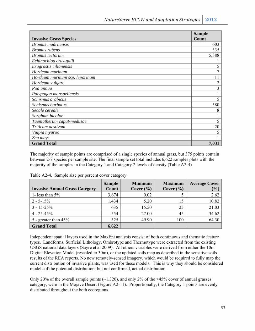
NatureServe HCCVI and Adaptation Strategies 2012
53
Invasive Grass Species Sample Count
Bromus madritensis 603Bromus rubens 335Bromus tectorum 5,388Echinochloa crus-galli 1Eragrostis cilianensis 5Hordeum murinum 7Hordeum murinum ssp. leporinum 11Hordeum vulgare 2Poa annua 3Polypogon monspeliensis 1Schismus arabicus 5Schismus barbatus 580Secale cereale 8Sorghum bicolor 1Taeniatherum caput-medusae 5Triticum aestivum 20Vulpia myuros 5Zea mays 1Grand Total 7,031
The majority of sample points are comprised of a single species of annual grass, but 375 points contain between 2-7 species per sample site. The final sample set total includes 6,622 samples plots with the majority of the samples in the Category 1 and Category 2 levels of density (Table A2-4).
Table A2-4. Sample size per percent cover category.
Invasive Annual Grass Category Sample Count
Minimum Cover (%)
Maximum Cover (%)
Average Cover (%)
1- less than 5% 3,674 0.02 5 2.622 - 5-15% 1,434 5.20 15 10.823 - 15-25% 635 15.50 25 21.034 - 25-45% 554 27.00 45 34.625 - greater than 45% 325 49.90 100 64.30Grand Total 6,622
Independent spatial layers used in the MaxEnt analysis consist of both continuous and thematic feature types. Landforms, Surficial Lithology, Ombrotype and Thermotype were extracted from the existing USGS national data layers (Sayre et al 2009). All others variables were derived from either the 10m Digital Elevation Model (rescaled to 30m), or the updated soils map as described in the sensitive soils results of the REA reports. No new remotely-sensed imagery, which would be required to fully map the current distribution of invasive plants, was used for these models. This is why they should be considered models of the potential distribution; but not confirmed, actual distribution. Only 20% of the overall sample points (~1,320), and only 2% of the >45% cover of annual grasses category, were in the Mojave Desert (Figure A2-11). Proportionally, the Category 1 points are evenly distributed throughout the both ecoregions.
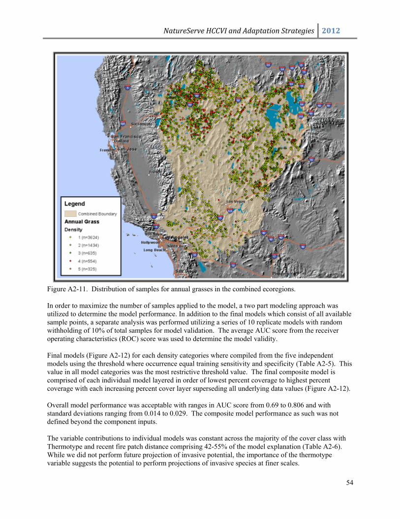
NatureServe HCCVI and Adaptation Strategies 2012
54
Figure A2-11. Distribution of samples for annual grasses in the combined ecoregions. In order to maximize the number of samples applied to the model, a two part modeling approach was utilized to determine the model performance. In addition to the final models which consist of all available sample points, a separate analysis was performed utilizing a series of 10 replicate models with random withholding of 10% of total samples for model validation. The average AUC score from the receiver operating characteristics (ROC) score was used to determine the model validity. Final models (Figure A2-12) for each density categories where compiled from the five independent models using the threshold where occurrence equal training sensitivity and specificity (Table A2-5). This value in all model categories was the most restrictive threshold value. The final composite model is comprised of each individual model layered in order of lowest percent coverage to highest percent coverage with each increasing percent cover layer superseding all underlying data values (Figure A2-12). Overall model performance was acceptable with ranges in AUC score from 0.69 to 0.806 and with standard deviations ranging from 0.014 to 0.029. The composite model performance as such was not defined beyond the component inputs. The variable contributions to individual models was constant across the majority of the cover class with Thermotype and recent fire patch distance comprising 42-55% of the model explanation (Table A2-6). While we did not perform future projection of invasive potential, the importance of the thermotype variable suggests the potential to perform projections of invasive species at finer scales.
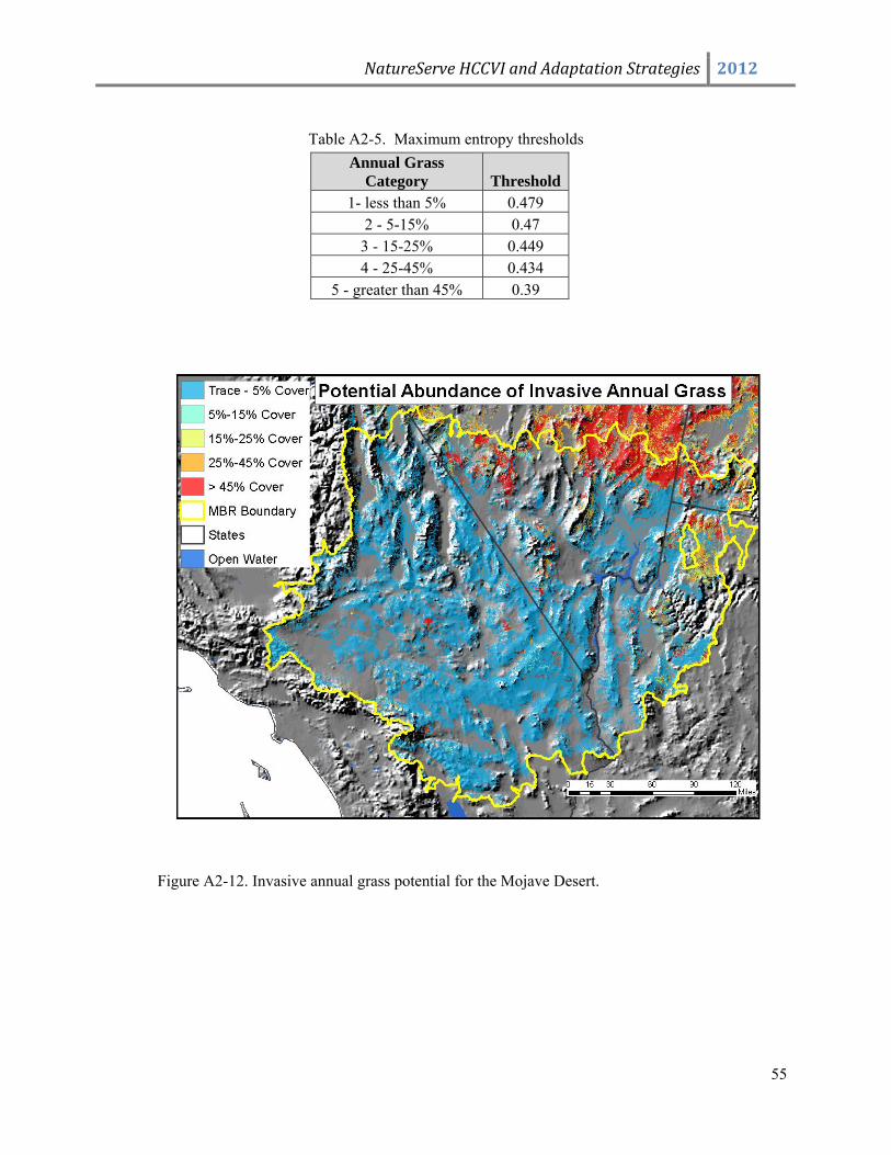
NatureServe HCCVI and Adaptation Strategies 2012
55
Table A2-5. Maximum entropy thresholds
Annual Grass Category Threshold
1- less than 5% 0.479 2 - 5-15% 0.47
3 - 15-25% 0.449 4 - 25-45% 0.434
5 - greater than 45% 0.39
Figure A2-12. Invasive annual grass potential for the Mojave Desert.
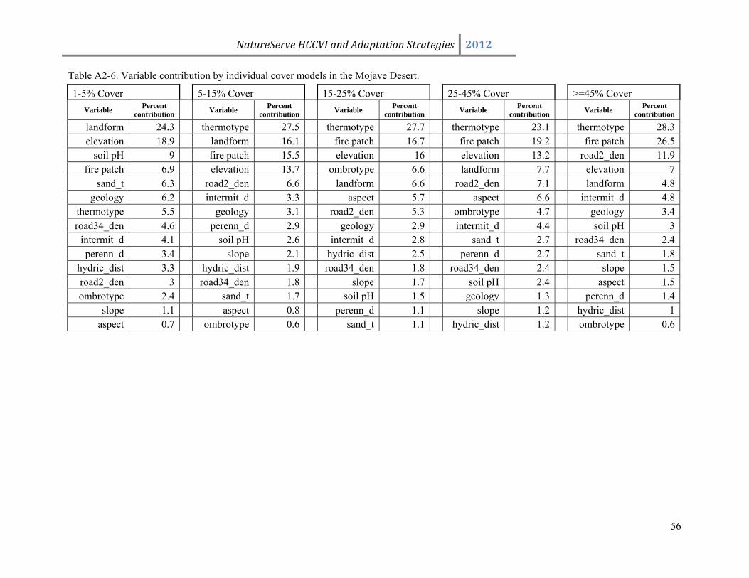
NatureServe HCCVI and Adaptation Strategies 2012
Table A2-6. Variable contribution by individual cover models in the Mojave Desert.
1-5% Cover 5-15% Cover 15-25% Cover 25-45% Cover >=45% Cover Variable Percent
contribution Variable Percent
contribution Variable Percent
contribution Variable Percent
contribution Variable Percent
contribution
landform 24.3 thermotype 27.5 thermotype 27.7 thermotype 23.1 thermotype 28.3elevation 18.9 landform 16.1 fire patch 16.7 fire patch 19.2 fire patch 26.5
soil pH 9 fire patch 15.5 elevation 16 elevation 13.2 road2_den 11.9fire patch 6.9 elevation 13.7 ombrotype 6.6 landform 7.7 elevation 7
sand_t 6.3 road2_den 6.6 landform 6.6 road2_den 7.1 landform 4.8geology 6.2 intermit_d 3.3 aspect 5.7 aspect 6.6 intermit_d 4.8
thermotype 5.5 geology 3.1 road2_den 5.3 ombrotype 4.7 geology 3.4road34_den 4.6 perenn_d 2.9 geology 2.9 intermit_d 4.4 soil pH 3
intermit_d 4.1 soil pH 2.6 intermit_d 2.8 sand_t 2.7 road34_den 2.4perenn_d 3.4 slope 2.1 hydric_dist 2.5 perenn_d 2.7 sand_t 1.8
hydric_dist 3.3 hydric_dist 1.9 road34_den 1.8 road34_den 2.4 slope 1.5road2_den 3 road34_den 1.8 slope 1.7 soil pH 2.4 aspect 1.5ombrotype 2.4 sand_t 1.7 soil pH 1.5 geology 1.3 perenn_d 1.4
slope 1.1 aspect 0.8 perenn_d 1.1 slope 1.2 hydric_dist 1aspect 0.7 ombrotype 0.6 sand_t 1.1 hydric_dist 1.2 ombrotype 0.6
56
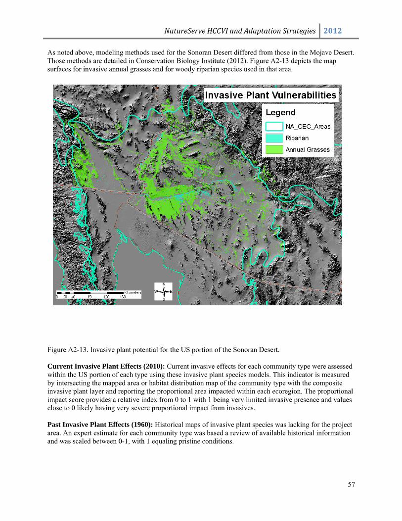
NatureServe HCCVI and Adaptation Strategies 2012
57
As noted above, modeling methods used for the Sonoran Desert differed from those in the Mojave Desert. Those methods are detailed in Conservation Biology Institute (2012). Figure A2-13 depicts the map surfaces for invasive annual grasses and for woody riparian species used in that area.
Figure A2-13. Invasive plant potential for the US portion of the Sonoran Desert.
Current Invasive Plant Effects (2010): Current invasive effects for each community type were assessed within the US portion of each type using these invasive plant species models. This indicator is measured by intersecting the mapped area or habitat distribution map of the community type with the composite invasive plant layer and reporting the proportional area impacted within each ecoregion. The proportional impact score provides a relative index from 0 to 1 with 1 being very limited invasive presence and values close to 0 likely having very severe proportional impact from invasives. Past Invasive Plant Effects (1960): Historical maps of invasive plant species was lacking for the project area. An expert estimate for each community type was based a review of available historical information and was scaled between 0-1, with 1 equaling pristine conditions.
NatureServe HCCVI and Adaptation Strategies 2012
58
LITERATURE CITED Anderson, M. D. 2001c. Coleogyne ramosissima. In: Fire Effects Information System [Online]. USDA Forest Service, Rocky Mountain Research Station, Fire Sciences Laboratory (Producer). [http://www.fs.fed.us/database/feis/] (accessed 2 January 2011). Abatzoglou, J.T., and C.A. Kolden. 2011. Climate Change in Western Deserts: Potential for increased wildlife and invasive annual grasses. Rangeland Ecology and Management. 64(5): 471-478. Archer, S.R., and K.I. Perlick. 2008. Climate Change and Ecosystems of the Southwest United States. Ranglands (June 2008) Society for Range Management. Blackburn, W. H., and P. T. Tueller. 1970. Pinyon and juniper invasion in black sagebrush communities in east-central Nevada. Ecology 51:841-848. Bowers, J.E. 1982. The plant ecology of inland dunes in western North America. Journal of Arid Environments 5:199-220. Bowers, J.E. 1984. Plant geography of southwestern sand dunes. Desert Plants 6(1):31-42, 51-54. Brooks, M.L., T. C Esque, and T. Duck. 2007. Creosote, Blackbrush, and Interior Chaparral Shrublands. In: USDA Forest Service Gen. tech Rep. RMRS-GTR-202. pp. 97-110. Brown M.T. and M.B. Vivas. 2005. Landscape Development Intensity Index. Environmental Monitoring and Assessment. 101:289-309. Brown, R. D., and P. W. Mote. 2009. The response of Northern Hemisphere snow cover to a changing climate. Journal of Climate 22:2124-2145. Brown, T. J., B. L. Hall, and A. L. Westerling. 2004. The impact of twenty-first century climate change on wildland fire danger in the western United States: An applications perspective. Climatic Change 62:365-388. Cayan, D. R., T. Das, D. W. Pierce, T. P. Barnett, M. Tyree, and A. Gershunov. 2010. Future dryness in the southwest U.S. and the hydrology of the early 21st century drought. Proceedings of the National Academy of Sciences 107(50):21271-21276. Online: www.pnas.org/cgi/doi/10.1073/pnas.0912391107 Chambers, J. C., E. D. McArthur, S. B. Monson, S. E. Meyer, N. L. Shaw, R. J. Tausch, R. R. Blank, S. Bunting, R. R. Miller, M. Pellant, B. A. Roundy, S. C. Walker, and A. Whittaker. 2005. Sagebrush Steppe and Pinyon-Juniper Ecosystems - Effects of Changing Fire Regimes, Increased Fuel Loads, and Invasive Species. Joint Fire Sciences Report Project #00-1-1-03. Chambers, J. C., and M. Pellant. 2008. Climate change impacts on northwestern and intermountain United States. Rangelands:29-33. Chambers, J. C., and M. J. Wisdom. 2009. Priority research and management issues for the imperiled Great Basin of the western United States. Restoration Ecology 17(5):707-714.
NatureServe HCCVI and Adaptation Strategies 2012
59
Comer, P.J. & J Hak. 2009. NatureServe Landscape Condition Model. Technical documentation for NatureServe Vista decision support software engineering. NatureServe, Boulder CO. Comer and Hak (in prep.2012) Modeling Landscape Condition in the Western United States: methods and results for application for measuring landscape integrity. for submittal to peer-review journal. Comer, P.J., P.J. Crist, M.S. Reid, J. Hak, H. Hamilton, B. Unnasch, I. Varley, D. Braun, G. Kittel., S. Auer, D. Theobald, D. Richards, and L. Kutner. 2012. A Rapid Ecoregional Assessment of the Mojave Basin and Range Ecoregion. Report, appendices, and databases provided to the Bureau of Land Management. Conservation Biology Institute. 2012. A Rapid Ecoregional Assessment of the Sonoran Desert Ecoregion. Draft report, appendices, and databases provided to the Bureau of Land Management. Christensen, N. S., and D. P. Lettenmaier. 2007. A multimodel ensemble approach to assessment of climate change impacts on the hydrology and water resources of the Colorado River Basin. Hydrology and Earth System Sciences 11:1417-1434. Covich, A. P. 2009. Emerging Climate Change Impacts on Freshwater Resources: A Perspective on Transformed Watersheds. A Resources for the Future (RFF) Report, June 2009. Online: www.rff.org/rff/documents/RFF-Rpt-Adaptation-Covich.pdf. Das, T., H. G. Hidalgo, M. D. Dettinger, D. R. Cayan, D. W. Pierce, C. Bonfils, T. P. Barnett, G. Bala, and A. Mirin. 2009. Structure and detectability of trends in hydrological measures over the western United States. Journal of Hydrometeorology 10:871:892. Dettinger, M., H. Hidalgo, T. Das, D. Cayan, and N. Knowles. 2009. Projections of potential flood regime changes in California. Report CEC-500-2009-050-F by the California Climate Change Center for the California Energy Commission (CEC) and the California Environmental Protection Agency (Cal/EPA). ESSA Technologies Ltd. 2007. Vegetation Dynamics Development Tool User Guide, Version 6.0. Prepared by ESSA Technologies Ltd., Vancouver, BC. 196 pp. Esque, T.C., C.R. Schwalbe, D.F. Haines and W.L. Halvorson. 2004. Saguaros under siege: invasive species and fire. Desert Plants 20(1): 49-55. Field, C. B., G. C. Daily, F. W. Davis, S. Gaines, P. A. Matson, J. Melack, and N. L. Miller. 1999. Confronting Climate Change in California: Ecological Impacts on the Golden State. Union of Concerned Scientists, Cambridge, MA, and Ecological Society of America, Washington, DC. Forman, R.T.T. and L.E. Alexander. 1998. Roads and their major ecological effects. Annual Review in Ecology and Systematics 8:629-644. Forman, S. L., M. Spaeth, L. Marin, J. Pierson, J. Gomez, F. Bunch, and A. Valdez. 2006. Episodic late Holocene dune movements on the sand-sheet area, Great Sand Dunes National Park and Preserve, San Luis Valley, Colorado, USA. Quaternary Reserearch 66:97-108. Gucker, C. L. 2006a. Yucca brevifolia. In: Fire Effects Information System [Online]. USDA Forest Service, Rocky Mountain Research Station, Fire Sciences Laboratory (Producer). [http://www.fs.fed.us/database/feis/] (accessed 2 January 2011).
NatureServe HCCVI and Adaptation Strategies 2012
60
Gucker, C. L. 2006b. Yucca schidigera. In: Fire Effects Information System [Online]. USDA Forest Service, Rocky Mountain Research Station, Fire Sciences Laboratory (Producer). [http://www.fs.fed.us/database/feis/] (accessed 2 January 2011). Hamerlynck, E. P., J. R. McAuliffe, E. V. McDonald, and S. D. Smith. 2002. Ecological response of two Mojave Desert shrubs to soil horizon development and soil water dynamics. Ecology 83:768-779. Hansen, A. J., R. L. Knight, J. M. Marzluff, S. Powell, K. Brown, P. H. Gude, and K. Jones. 2005. Effects of exurban development on biodiversity: patterns, mechanisms, and research needs. Ecological Applications 15:1893–1905. Harper, M. P., and B. L. Peckarsky. 2006. Emergence cues of a mayfly in a high-altitude stream ecosystem: Potential response to climate change. Ecological Applications 16(2):612-621. Hultine, K. R., S. E. Bush, A. G. West, and J. R. Ehleringer. 2007. Population structure, physiology and ecohydrological impacts of dioecious riparian tree species of western North America. Oecologia 154(1):85-93. Online: DOI 10.1007/s00442-007-0813-0. Isaak, D. J., C. H. Luce, B. E. Rieman, D. E. Nagel, E. E. Peterson, D. L. Horan, S. Parkes, and G. L. Chandler. 2010. Effects of climate change and wildfire on stream temperatures and salmonid thermal habitat in a mountain river network. Ecological Applications 20(5):1350-1371. Jackson, S. T., J. L. Betancourt, R. K. Booth, and S. T. Gray. 2009. Ecology and the ratchet of events: Climate variability, niche dimensions, and species distributions. Proceedings of the National Academy of Sciences 106, supplement 2:19685-19692. Online: www.pnas.org_cgi_doi_10.1073_pnas.0901644106. Jager, H. I., W. Van Winkle, and B. D. Holcomb. 1999. Would hydrologic climate changes in Sierra Nevada streams influence trout persistence? Transactions of the American Fisheries Society 128:222–240. Keane, R. E., T. L. Frescino, M. C. Reeves, and J. Long. 2006. Mapping wildland fuels across large regions for the LANDFIRE prototype project. Pages 367-396 in: M. G. Rollins and C. Frame, editors. The LANDFIRE Prototype Project: Nationally consistent and locally relevant geospatial data for wildland fire management. General Technical Report RMRS-GTR-175. USDA Forest Service, Rocky Mountain Research Station, Fort Collins, CO. Keeler-Wolf, T. 2007. Mojave Desert scrub vegetation. Pages 609-656 in: M. G. Barbour, T. Keeler-Wolf, and A. A. Schoenherr, editors. 2007. Terrestrial vegetation of California. Third edition. University of California Press, Berkeley. Keeler-Wolf, T., C. Roye, and K. Lewis. 1998. Vegetation mapping and classification of the Anza-Borrego Desert State Park, California. Unpublished report on file at California Natural Diversity Database, California Department Fish and Game, Sacramento. Keeler-Wolf. T., and X. Thomas. 2000. Draft descriptions of vegetation alliances for the Mojave Ecosystem Mapping project. California Natural Diversity Database, California Department of Fish and Game, Sacramento. Knick, S. T., and J. T. Rotenberry. 1995. Landscape characteristics of fragmented shrub steppe habitats and breeding passerine birds. Conservation Biology 9:1059–1071.
NatureServe HCCVI and Adaptation Strategies 2012
61
Leu, M., S. E. Hanser and S. T. Knick. 2008. The human footprint in the West: a large-scale analysis of anthropogenic impacts. Ecological Applications 18:1119–1139. Lowry, J. R.D. Ramsey, K. Thomas, D. Schrupp, T. Sajwaj, J. Kirby, E. Waller, S. Schrader, S. Falzarano, L. Langs, G. Manis, C. Wallace, K. Schulz, P. Comer, K. Pohs, W. Rieth, C. Velasquez, B. Wolk, W. Kepner, K. Boykin, L. O’Brian, D. Bradford, B. Thompson, and J. Prior-Magee. 2007. Mapping moderate-scale land-cover over very large geographic areas within a collaborative framework: a case study of the Southwest Regional Gap Analysis Project (SWReGAP). Remote Sensing and Environment 108: 59-73. Martin, T. E. 2007. Climate correlates of 20 years of trophic changes in a high-elevation riparian system. Ecology 88(2):367-380. McCabe, G. J., and D. M. Wolock. 2009. Recent declines in western U.S. snowpack in the context of twentieth-century climate variability. Earth Interactions 13(12):1-15. McClaran, M.P. and T.R. VanDevender, eds. 1995. The Desert Grassland. University of Arizona Press. Tucson. McLaughlin, S.P. and J.E. Bowers. 1982. Effects of fire on a Sonoran Desert community. Ecology 63: 246-248. Meinzer, F. C., C. S. Wisdom, A. Gonzales-Coloma, P. W. Rundel, and L. M. Shultz. 1990. Effects of leaf resin on stomatal behavior and gas exchange of Larrea tridentata. Functional Ecology 4:579-584. Melack, J. M., J. Dozier, C. R. Goldman, D. Greenland, A. M. Milner, and R. J. Naiman. 1997. Effects of climate change on inland waters of the Pacific coastal mountains and western Great Basin of North America. Hydrological Processes 11:971-992. Miller, D. M., S. P. Finn, A. Woodward, A. Torregrosa, M. E. Miller, D. R. Bedford, and A. M. Brasher. 2010. Conceptual ecological models to guide integrated landscape monitoring of the Great Basin. U.S. Geological Survey, Scientific Investigations Report 2010-5133. Reston, VA. Minnich, R. A. 2007. Southern California conifers. Pages 502-538 in: M. G. Barbour, T. Keeler-Wolf, and A. A. Schoenherr, editors. Terrestrial vegetation of California. Third edition. University of California Press, Berkeley. Mote, P. W. 2006. Climate-driven variability and trends in mountain snowpack in western North America. Journal of Climate 19:6209-6220. Munson, S.M., R.H. Webb, J. Belnap, J.A. Hubbard, D.E. Swann, and S. Rutman. 2011. Forecasting climate change impacts to p[lant community composition in the Sonoran Desert region. Global Change Biology (2011), doi:10.1111/j.1365-2486.2011.02598.x Phillips, S.J., R.P. Anderson, and R.E. Schapire. 2006. Maximum entropy modeling of species geographic distributions. Ecological Modeling. Vol. 190 (3–4): 231–25 PRISM data (http://www.prism.oregonstate.edu/ ) Provencher, L., and T. Anderson. 2011. Climate Change Revisions to Nevada’s Wildlife Action Plan: Vegetation Mapping and Modeling. Report to the Nevada Department of Wildlife
NatureServe HCCVI and Adaptation Strategies 2012
62
Raffa, K. F., B. H. Aukema, B. J. Bentz, A. L. Carroll, J. A. Hicke, M. G. Turner, and W. H. Romme. 2008. Cross-scale drivers of natural disturbances prone to anthropogenic amplification: Dynamics of biome-wide bark beetle eruptions. BioScience 58:501-517. Rivas-Martinez, S., D. Sanchez-Mata, And M. Costa. 1999. North American Boreal and Western Temperate Forest Vegetation. Itinera Geobotanica 12:5-316. Riitters, K. H., and J. D. Wickham. 2003. How far to the nearest road? Frontiers in Ecology and the Environment 1:125–129. Rivera, S., N. E. West, A. J. Hernandez, and R. D. Ramsey. 2011. Predicting the impact of climate change on cheat grass (Bromus tectorum) invasibility for northern Utah: A GIS and remote sensing approach. Natural Resources and Environmental Issues 17(13). Rocchio, F. J. and R. C. Crawford. 2011. Applying NatureServe’s Ecological Integrity Assessment Methodology to Washington’s Ecological Systems. Washington Natural Heritage Program, Washington Department of Natural Resources, Olympia, Washington. Rollins, M. G., and C. Frame. 2006. The LANDFIRE Prototype Project: Nationally consistent and locally relevant geospatial data for wildland fire management. General Technical Report RMRS-GTR-175. USDA Forest Service, Rocky Mountain Research Station, Fort Collins, CO. Sanderson, E. W., M. Jaiteh, M. A. Levy, K. H. Redford, A. V. Wannebo, and G. Woolmer. 2002. The human footprint and the last wild. BioScience 52:891–904. Sawyer, J. O., T. Keeler-Wolf, and J. Evens. 2009. A manual of California vegetation. Second edition. California Native Plant Society, Sacramento CA. 1300 pp. Sayre, R., P. Comer, H. Warner, and J. Cress. 2009. A new map of standardized terrestrial ecosystems of the conterminous United States, U.S. Geological Survey Professional Paper 1768. Schwinning, S., B. I. Starr, and J. R. Ehleringer. 2003. Summer and winter drought in a cold desert ecosystem (Colorado Plateau). Part 1: Effects on soil water and plant water uptake. Journal of Arid Environments 60(4):547-566. Seavy, N. E., T. Gardali, G. H. Golet, F. T. Griggs, C. A. Howell, R. Kelsey, S. L. Small, J. H. Viers, and J. F. Weigand. 2009. Why climate change makes riparian restoration more important than ever: Recommendations for practice and research. Ecological Restoration 27(3):330-338. Seiler, A. 2001. Ecological Effects of Roads, A review. Introductory Research Essay No. 9. Department of Conservation Biology, Swedish University of Agricultural Science, Upsalla. Tausch, R. J., N. E. West, and A. A. Nabi. 1981. Tree age and dominance patterns in Great Basin pinyon-juniper woodlands. Journal of Range Management 34(4):259-264. Tausch, R. J., and N. E. West. 1988. Differential establishment of pinyon and juniper following fire. The American Midland Naturalist 119(1):174-184. Theobald, D. M. 2001. Land-use dynamics beyond the American urban fringe. Geographical Review 91:544–564.
NatureServe HCCVI and Adaptation Strategies 2012
63
Theobald, D. 2010. Estimating natural landscape changes from 1992 to 2030 in the conterminous US. Landscape Ecology 25:999–1011 Thorn, R. F., A.A. Schoenherr, C.D. Clements, and J.A. Young. 2007. Transmontane Coniferous Vegetation. In Barbour, Michael G., Todd Keeler-Wolf, and Allan A. Schoenherr. Terrestrial Vegetation of California. Third Edition. Berkeley, CA: University of California Press, 2007. pp 574-586. Trombulak, S. C., and C. A. Frissel. 1999. Review of ecological effects of roads on terrestrial and aquatic communities. Conservation Biology 14:18–30. USBOR [U.S. Bureau of Reclamation]. 2011. Reclamation, SECURE Water Act Section 9503(c) - Reclamation Climate Change and Water, Report to Congress, 2011. Report prepared for the United States Congress by the U.S. Department of the Interior Bureau of Reclamation, April 2011. U.S. Environmental Protection Agency. 2001. Southeastern US Ecological Framework Project. Online at: http://www.geoplan.ufl.edu/epa/index.html US Global Change Research Program. 2009. Global Climate Change Impacts in the United States. Thomas R. Karl, Jerry M. Melillo, and Thomas C. Peterson (eds.). United States Global Change Research Program. Cambridge University Press, New York, NY, USA. Vasek, F. C. 1980. Creosote bush: Long-lived clones in the Mojave Desert. American Journal of Botany 67:246-255. Vogelmann, J. E., J. R. Kost, B. Tolk, S. Howard, K. Short, X. Chen, C. Huang, K. Pabst, and M. G. Rollins. 2011. Monitoring landscape change for LANDFIRE using multi-temporal satellite imagery and ancillary data. Journal of Selected Topics in Applied Earth Observations and Remote Sensing 4(2):252-264. Wangler, M. J., and R. A. Minnich. 2006. Fire succession in pinyon-juniper woodlands in the San Bernardino Mountains. Madrono 43:493-514. Weisberg P. J., E, Lingua, and R. B. Pillai. 2007. Spatial patterns of pinyon-juniper woodland expansion in central Nevada. Rangeland Ecology and Management 60:115-124. Westerling, A. L., H. G. Hidalgo, D. R. Cayan, and T. W. Swetnam. 2006. Warming and earlier spring increase western U.S. wildfire activity. Science 313:940-943. Zouhar, K. L. 2001b. Pinus monophylla. In: Fire Effects Information System [Online]. USDA Forest Service, Rocky Mountain Research Station, Fire Sciences Laboratory (Producer). [http://www.fs.fed.us/database/feis/] (accessed 2 January 2011).