Embed Size (px)
Citation preview

NASA Contractor Report 172466
ICASE REPORT NO. 84-47NASA-CR- 172466
19850003261
/:
: ICASEPARALLEL TRIANGULARIZATION OF SUBSTRUCTUREDFINITE ELEMENT PROBLEMS
Michael R. Leuze
LiB_A_Voopvi.:-.J:i_o 1984
Contract No, NASt-t7130LANGLEYRESEARCHCENTER
September 1984 LIBRARY,NASA_,_PTON_,. VIRGINIA
INSTITUTE FOR COMPUTER APPLICATIONS IN SCIENCE AND ENGINEERINGNASA Langley Research Center, Hampton, Virginia 23665
, Operated by the Universities Space Research Association
N/kSANationalAeronautics andSpaceAdministration
Langley Ros_rch CorttorHampton.Virginia 23665
https://ntrs.nasa.gov/search.jsp?R=19850003261 2018-06-02T08:20:28+00:00Z

U ID_'LHT 1"-_./ .El 1
• ._c.:,: .. F:PT ._,_ 172-'-'.:,'-g5N{ i ....... .... -_t.-_.---_-_...._,,-.x.,,----,-- ,--,A ._-_ _tA,'-- ._ _,"- _"_,-'_-"-'- P__J.T--_--: _IA'_4 _.-'ti,_.,,T.: F..-'-,- MP"-" "_" ,-,.r-..-,--..-_ "-''_ ""-"- ;'J3.O.
it: _H_:L._. L:F,,ILLHJ3 : i'- i EL: L:ULLTIE._'I i
vTTL: P_--'" '_" "_- -'rr =!'" -'Y -:=-'t='un " o_b _ructured T ill1 I.E -'_'I_£'IyEI31. i-:Kt_b}_3111__]",,' ,_}, " t ..... i ..... -- OT .... :S. ................................TL_ -_ - -:........
HUIII; H, LLUZ_L, i':i. R. r ................... t ...... )
C'-'RP- N......... " ....... " " ":slratior_ ...................v ; : a :. _ o[M _ HerORSU _ i ._"-S aRd c_._:.__ nu,:: :,, . 'L_:,:, =z" _:_====, ._:,"_" LE:R" _[_r,
H t V ............. cAP .... . .a_ ........'..1: dill :j _Jii_ el. r_-.niL. 1_ii i_ .Jr. _.. r_vr_, :-n H:31
F'.'_.'c: .i_C0_.,.._,.,.TZ-.. ,:O_.j.,_:c._-.._ ,'z. __=.-:E:_,.,Tb'---u..'-I,'_;.sB_R .... ,z. up..,a..tj_,=c_.._:C ..............M._._ N_U,_T, , , I, .TE _LE..... "IET,I_D. ,_. "_LL_L PR,_ES_'[': _....•"..'_U[:I_U i LI-<_.." / ""
i"n,'.,i : igi'_3 ".I_iHI_ILFIHI IL_,)/"STIr,'-NES._ _4HTI-<IX
- u-.=vn _ ,.v_,=.-,-I-K:JBLE...--I_:JL'4 1T_:m
HBH; f HM LIIL_F
H._; .M:JU}I :aT [he .COi:..:._U_dtiO..'_dl efT-_rt O_ the #inlLe ele.:.:..'ei_ FrOC#£_ ir:volve£
LiliI_ _"_JMEII[_:j :,_, m,_}_'_ ;.hi5 i5:_'5[eiii 15 SUL=S_ _-LrUCT.UY i r_ OY .Fii_"-:"::._.
.. tl [;c,n_..'_. Substruutur;..':._ =.a b_sed c,r [,_ ;dea _T u_v_d..'n_ = a_ru.z:-ureir_O ..................... "_-............ -:.... "-_'e_uh -,T_i_ci_ c_n - = nde.=_nen'}';-'.._--_.ue_, _h_:n = -ana_:-.;ed re,_t ..... i ..........
d t, =t ........ L ..... t b t ............"'_,_ _'=_'':Z-" {:-'_']-'--"""" ..:............._ "_''_ 1:31" a...... _.._.__ _..-_'_.T _ _J.


, PARALLEL TRIANGULARIZATION
OF SUBSTRUCTURED FINITE ELEMENT PROBLEMS
Michael R. Leuze
Vanderbilt University
Abstract
Much of the computational effort of the finite element process in-volves the solution of a system of linear equations. The coefficient
matrix of this system, known as the global stiffness matrix, issymmetric, positive definite, and generally sparse. An importanttechnique for reducing the time required to solve this system issubstructuring or matrix partitioning. Substructuring is based onthe idea of dividing a structure into.pieces, each of which can thenbe analyzed relatively independently. As a result of this division,each point in the finite element discretization is either interior to
a substructure or on a boundary between substructures. Contri-butions to the global stiffness matrix from connections between
boundary points form the Kbb matrix. This paper focuses on thetriangularization of a general I_bb matrix on a parallel machine.
Support for this research was provided in part by the National Aeronautics and
Space Administration under contract number NASI-17130 while the author was in
residence at ICASE, NASA Langley Research Center, Hampton, VA 23665, and inpart by the National Science Foundation under Grant No. MCS-8305693.
I. Introduction
The finiteelementmethodisan importanttoolfordeterminingapproximate
solutionstosystemsofdifferentialequationsarisinginsuchdiversephysicalprob-lemsasstructuralanalysis,fluidflow,and heattransport.In thefiniteelement
approach,a regionofinterest(e.g.,an airplanewing,a crosssectionofa pipe,ora nuclearreactorcore)isdiscretizedintoindividualelements.The solutionthen
givesdisplacements,vorticities,ortemperaturesatthosepointswheretwoormore
elementsarejoinedtogether.A completedescriptionofthemethodhasappeared
numeroustimesintheliterature,cf.[7].Much ofthecomputationaleffortofthefiniteelementprocessinvolvesthesolutionofasystemoflinearequations.The co-
efficientmatrixofthissystem,known astheglobalstiffnessmatrix,issymmetric,
positivedefinite,and generallysparse.To reducethetimerequiredtosolvethis
system, reseaz:chershave examined many techniques, among which is Substructuringor matrix partitioning, cf. [6].
Substructuring is based on the idea of dividing a structure into pieces, whichcan then be analyzed relatively independently. As a result of this division, each
point in the discretization is either interior to a substructure or on a boundary be-tween substructures. The application of substructuring techniques has two obviousadvantages. First, if the finite element method is applied to a structure, and aportion of that structure is then changed in some way, only interior and boundarypoints of the substructures which have changed need to be reexamined. This is anadvantage, for example, in the case of a researcher considering aircraft structure
who wishes to fit a new wing to an existing model. Second, with the increased avail-ability of parallel processors, substructuring is a natural way to decompose a finiteelement problem into relatively independent subproblems. A separate processorcan then be applied to the solution of each subproblem.
The discretization process in the finite element method gives rise to a graph ina very natural way. Points where two or more elements join together are the verticesor nodes of the graph; two nodes which border on a common element are joined byan edge. The structure of the global stiffness matrix is dependent upon the orderingof the nodes in this finite element graph and is, in fact, equivalent to the structure
of the graph's adjacency matrix. If the nodes corresponding to interior points arenumbered first, one substructure at a time, followed by the nodes correspondingto boundary points, the global stiffness matrix will have the form of the matrix in
Figure 1, where K_ ") represents the contributions from connections between interiorr_,-(i)and K_ ) represent the connections between interiorpoints of substructure j, "*hi
2

pointsofsubstructurej and the setofboundary points,and K_ representsthe
contributionsfrom boundary-to-boundaryconnections.
•
Kb ) - (_) n-€")i
Figure I. GlobalStiffnessMatrixStructure
The question of the amount of parallelism inherent in the finite element process
• as a whole has been examined, cf. [1]. The focus of this paper is the triangularizationof a general Kbb matrix on a parallel machine. This portion of the problem is of
considerable importance for at least two reasons. First, if any part of the structure
or region of interest is changed, at least a portion of the Kbb matrix must be re-
triangularized. Second, as the number of processors in parallel machines increases,there will be a tendency to partition structures into more substructures• As the
number of substructures increases, so does the relative number of boundary points
and thus the relative size of the Kbb matrix.
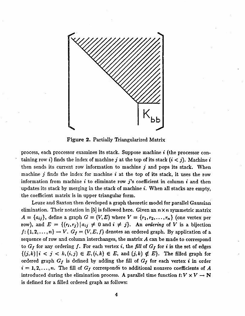
It is assumed that during the solution of the system of linear equations required
by the finite element process, the global stiffness matrix has been reduced by means
of Gaussian elimination to the form of the matrix in Figure 2, so that only the Kbb
matrix is yet to be triangularized.
2. ParallelGaussian Elimlnation
The orderingoftherows and columnsofa givenmatrix(orequivalently,the
orderingofthe nodes in the correspondinggraph)requiredto minimizeparallel
. Gaussian elimination times has been studied by Leuze and Saxton [5]. Following
the development of their model, assume a completely connected parallel machine
- withan arbitrarilylargenumber ofprocessors.The triangularizationofa symmet-
ricsystemoflinearequationscouldbe programmed on sucha machineasfollows.
Each row isstoredin a separateprocessorasa listofnonzerocoefficientswith a
stackof correspondingcolumn indices•This stackindicatesto a processorwhat
communicationwith otherprocessorsisrequired.At eachstepofthe elimination
3
Kbb
Figure 2. Partially "Priangulaxized Matrix
process, each processor examines its stack. Suppose machine i (the processor con-
taining row i) finds the index of machine j at the top of its stack (i < j). Machine i
then sends its current row information to machine j and pops its stack. When
machine j finds the index for machine i at the top of its stack, it uses the row
information from machine i to eliminate row j's coefficient in column i and then
updates its stack by merging in the stack of machine i. When all stacks are empty,
the coefficient matrix is in upper triangular form.
Leuze and Saxton then developed a graph theoretic model for parallel Gaussian
elimination. Their notation in [5] is followed here. Given an n x n symmetric matrix
A = {aij}, define a graph G = (V,E) where V = {rl,r2,...,rn} (one vertex per
row), and E = {(ri, ri) [ai,i y£ 0 and i _ j}. An ordering of V is a bijection
f: {1, 2,..., n} --_ V. G$ = (V, E, f) denotes an ordered graph. By application of a
sequence of row and column interchanges, the matrix A can be made to correspond
to Gj- for any ordering f. For each vertex i, the fill of G$ for i is the set of edges
{(j,k)[i < j < k,(i,j) E E,(i,k) E E, and (3,k) _ E}. The filled graph for
ordered graph G$ is defined by adding the fill of G$ for each vertex i in orderi = 1, 2,..., n. The fill of G$ corresponds to additional nonzero coefficients of A
introduced during the elimination process. A parallel time function t: V × V _ N
is defined for a filled ordered graph as follows:
4
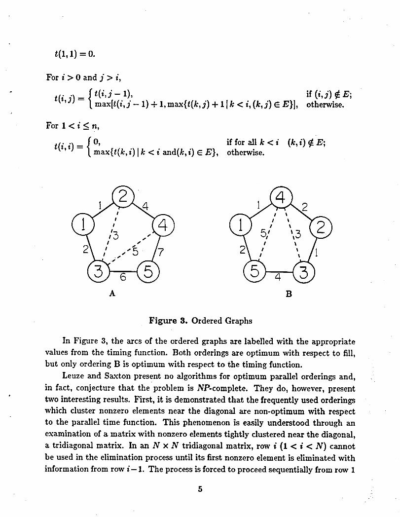
t(1,1)=o.
For i > 0 and j > i,
" ! t(i,j-- 1), if (i,j) _ E;t(i,j) = _ max[t(i,j-- 1)+ 1,max{t(k,j) + llk< i,(k,j) E E}], otherwise.
For l<i_n,
f0, if forallk<i (k,i)¢E;t(i,i) ( max{t(k,i)lk< i and(k,i)_E}, otherwise.
Figure 3. Ordered Graphs
In Figure 3, the arcs of the ordered graphs are labelled with the appropriatevalues from the timing function. Both orderings are optimum with respect to fill,but onlyorderingB is optimumwithrespectto the timingfunction.
Leuze and Saxton presentno algorithmsforoptimumparallelorderingsand,in fact, conjecturethat the problemis NP-complete. They do, however,present
° two interestingresults. First,it is demonstratedthat the frequentlyusedorderingswhich clusternonzerodements near the diagonalare non-optimumwith respectto the paralleltime function. This phenomenonis easily understoodthrough anexaminationof a matrixwith nonzeroelementstightly clusterednear the diagonal,a tridiagonalmatrix. In an N x N tridiagonalmatrix, rowi (1 < i < N) cannotbe used in the eliminationprocessuntil its firstnonzeroelementis eliminatedwithinformationfromrowi- 1. Theprocessis forcedto proceedsequentiallyfromrow1
5
to row N. Second, a system of linear equations which can be solved without fill
but for which any minimum parallel time ordering produces fill is presented. Thissystem demonstrates that in the parallel model, there is not a perfect correlationbetween the amount of fill and the number of time steps required to solve a system,as is the case in the sequential model.
In this paper, orderings for the class of Kbb matrices will be examined. The
special characteristics of the Kbb matrix will be examined in Section 3, heuristic or-derings applied to Kbb matrices will be discussed in Section 4, and parallel Gaussianelimination times resulting from the various orderings will be presented in Section 5.
3. The Structure of the Kbb Matrix
When attemptingtodeterminetheKbb matrixstructure,thefollowingobser-
vationaboutfillina symmetricmatrixisimportant.If,intheundirectedgraph
correspondingtomatrixA, thereexistsa pathbetweennodeiand nodej with
intermediatenodesnumberedlessthanrain{i,j},fillwilloccurinmatrixelements
AijandAjs',cf.[4],Ch.5.Consequently,iftheinteriornodesofasubstructureform
aconnectedset,eachboundarynodeofthatsubstructurewillbeconnected(either
originallyorby meansofafilledge)toeveryotherboundarynodeofthatsubstruc-
ture.Itthusseemsappropriatetodividethesetofboundarynodesintosubsetssuchthatallnodesinasubsetareboundarynodestothesamesetofsubstructures.
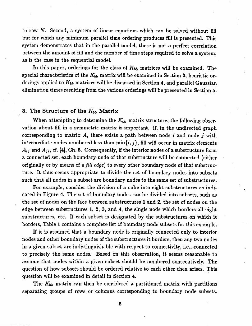
For example, consider the division of a cube into eight substructures as indi-cated in Figure 4. The set of boundary nodes can be divided into subsets, such asthe set of nodes on the face between substructures 1 and 2, the set of nodes on the
edge between substructures 1, 2, 3, and 4, the single node which borders all eight
substructures, etc. If each subset is designated by the substructures on which itborders, Table 1 contains a complete list of boundary node subsets for this example.
If it is assumed that a boundary node is originally connected only to interiornodes and other boundary nodes of the substructures it borders, then any two nodesin a given subset are indistinguishable with respect to connectivity, i.e., connectedto precisely the same nodes. Based on this observation, it seems reasonable toassume that nodes within a given subset should be numbered consecutively. Thequestion of how subsets should be ordered relative to each other then arises. Thisquestion will be examined in detail in Section 4.
The Kbb matrix can then be considered a partitioned matrix with partitionsseparating groups of rows or columns corresponding to boundary node subsets.
6

• . .- •.
. / 7/ 8//5/6
5 6
1 2
s
Figure 4. Substructured Cube
Table I.BoundaryNode Subsets
(1) 12 (7) 37 (13) 1234(2) 13 (8) 48 (1_) 1256(,5')15 (9) 56 (15) 1357(J) 24 (10) 57 (16) 2468(5) 26 (11) 68 (17) 3478(_)34 (1_)78 (18)5678
(19) 12345678
Sinceeachboundarynodeofa substructureisconnectedtoeveryotherboundary
nodeofthatsubstructure,theblocksresultingfromsuchapartitioningwilleitherbe
. composed entirely of nonzero elements or be composed entirely of zero elements. Ifthe "rowsubset" and "column subset" of a block share a common substructure, that
blockwillbe nonzero;otherwise,thatblockwillbe zero.Furthermore,whenever
filloccursduringthetriangularizationoftheKbb matrix,an entireblockwillbe
filled.Consequently,thestructureoftheKbbmatrixcanbe representedby amatrix
withonerowandonecolumnperboundarynodesubset,togetherwithinformation
aboutthesizeofeachsubset.Forexample,thesubdividedcubeofFigure4 with
7

theboundarynodesubsetorderingofTable1canbe representedby thematrixofFigure5.
Figure 5. Kbb MatrixStructure
InFigure5,a blacksquarerepresentsa nonzeroblock;awhitesquare,a zero
block.Blockdimensionscanbe determinedfromboundarysubsetsizes.Inthis
example,ifeachsubcube(includingboundarynodes)containsnsnodes,each"face"
(borderingon onlytwosubcubes)contains(n- 1)2 nodes,each"edge"(bordering
on foursubcubes)containsn - 1nodes,and thecentral_point"(borderingon alleightsubcubes)consistsofasinglenode.
4. Ordering Heuristics
Severalheuristicsfororderingboundarynode subsetswere appliedtotwo dif-
ferentstructures,a cubedividedinto27 subcubes,eachcontainingn3 nodes,and an
"airplane"(Figure6) constructedfrom92 squareplates,eachcontainingn2 nodes.
The substructureboundariesofthe cubewere dividedinto98 subsets;therewere
220 boundarynode subsetsfortheairplane.
For eachofthetwo structures,a ratherarbitrary"natural"ordering(Order-
ing0) ofboundarynode subsetswas initiallychosen.Subsetsofthecubewere di-
videdintothreecategories;all"faces"werenumbered first,followedby all"edges",
and finally,all"points".Allairplanesubsetscomposeda singlecategory.Withina
8
1 ........ •

Figure6.Structureof"Airplane_
category,boundarynodesubsetsborderingon substructure1werenumberedfirst,followedby unnumberedsubsetsborderingon substructure2,etc.
The orderingheuristicsdescribedbelowarebasedon twoobservationsofgen-eralgraphs.(Itshouldbe noted,however,thattheheuristicsareappliednotto
generalgraphs,butratherto graphswithverticesconsistingofsetsofboundarynodesindistinguishablewithrespecttoconnectivity.Blockreorderingsare,there-
fore,performedon thecorrespondingmatrices.)First,thetotalnumberofparalleltime steps is smaller for those orderings which number first those nodes adjacent to
relatively few other nodes. These graph orderings correspond to matrix orderingswhich number first those rows for which the least amount of work must be performedduring the elimination process. Thus, intuitively, work can begin on intermediaterows more quickly. Second, the total number of parallel time steps is larger for those
orderingswhichtendtonumberadjacentnodesconsecutively.Theseareorderingswhichclusternonzeroelementsofthematrixnearthediagonal.Numberingofthis
typeoccursintheCuthill-McKee[2]andreverseCuthill-McKee[3]orderings,whichareincludedforcomparison.
Ordering 1 (Cuthill-McKee):The firstsubsetinthenaturalordering
ischosenarbitrarilyas thestartingsubsetand assignedthenumber 1.
Then,fori--1,...,N (whereN isthetotalnumberofsubsets),findall
9

unnumbered subsets adjacent to subset i and number them in increasingorder of degree.
Ordering 2 (Reverse Cuthill-McKee): This ordering is obtained by re-versing the Cuthill-McKee ordering described above.
In the ordering descriptions that follow, two classes of variables, DEG andADJ, are associated with each subset.
DEG variables hold the degree of a subset, the number of subsets to which thatsubset is adjacent. By selecting the subset with minimum DEG value to be ordered
next, orderings which number subsets from lowest to highest degree are produced.DEGI contains the degree of a subset calculated a prior£ Its value does not changeduring the ordering process. Some ordering heuristics eliminate a subset when ithas been numbered and pairwise connect all subsets adjacent to this subset. DEG2
is dynamically updated to reflect the resulting changes in degree. The DEG2 value
of a subset is thus dependent upon the ordering selected and may increase as filloccurs or decrease as adjacent nodes are ordered and eliminated.
ADJ variables hold information about the set of numbered subsets to which
an unnumbered subset is adjacent. By selecting the subset with minimum ADJ
value to be ordered next, orderings which spread nonzero matrix elements, ratherthan cluster nonzero elements near the diagonal are produced. ADJI contains thecardinality of this set of numbered subsets; ADJ2 contains the maximum subset
number from this set. ADJ3 attempts to reflect both the set cardinality and themaximum value in the set. Whenever a subset i is numbered, for each unnumbered
adjacent subset j, ADJS(j) (initially zero) gets the value one plus the maximum ofADJS(i) and ADJS(j). ADJ4 is simply a flag which contains the value one if theset of adjacent numbered subsets is non-empty and the value zero otherwise. For
the problems considered, all ADJ$ flags were quickly set. Therefore, whenever itwas detected that all flags were set, all were reset to zero.
For each of the orderings, the variables of primary and secondary importanceare listed in Table 2. The unnumbered subset with minimum value for the variable of
primary importance is numbered next. Ties are broken by minimizing the variable of
secondary importance. Any remaining ties are broken by numbering first the subsetappearing earliest in the "natural" ordering. Orderings 8, 9, and 10 are equivalent
in a sense to the minimum degree algorithm [8],but correspond to matrix reorderingby blocks rather than individual elements.
10

Table 2. Heuristic Orderings
Primary Secondary- Ordering Variable Variable
3 DEG1 ADJ14 ADJI DEG1
5 ADJ2 DEG1
6 ADJ3 DEG1
7 ADJ_ DEG18 DEG2 --9 DEG£ ADJ1
10 DEG2 ADJ2
5. Testing
Each of the heuristic orderings for boundary node subsets was applied bothto the cube problem and to the airplane problem. For each ordering, parallel
Gaussian elimination as described in [5] was applied to the resulting Kbb matrix.The total number of parallel time steps, the maximum number of processors usedduring any one time step, and the average number of processors used per timestep were determined for various size problems. Values of n ranged from three to
nine (each subcube contained n3 nodes and each plate of the airplane containedn2 nodes). It did not appear necessary to examine larger problems because ofthe regularity of the data. For every test case, it was possible to determine acomplexity expression which exactly matched the parallel time step results for all
values of n greater than four. Processor usage results were not quite as regular overthe same range of values for n. Some complexity expressions appear to describe
exactly the asymptotic behavior of the maximum processor values; in other cases(marked by the symbol "_'), asymptotic behavior was not reached within the testrange. All maximum processor data was, however, of sufficient regularity to allowdetermination of the leading coefficient of the complexity expression with some
. degree of confidence. In addition, leading coefficients accurate to two decimal places
were calculated for complexity expressions describing average processor usage. Allcomplexity expressions are listed in Tables 3 and 4.
Actual values for parallel time steps and average number of processors for
selected orderings are plotted in Figures 7, 8, 9, and 10. Data for several orderingsare not plotted because the curves would lie extremely close to other curves which
11

Table 3. Complexity of Heuristic Orderings for Cube Problem
maximum averageOrdering Total steps processors processors
0 108n 2 -- 216n -F 109 ll.On 2 -l- O(n) 7.16n 2 + O(n)
1 108n 2 -- 216n -i- 109 18.0n 2 + O(n) 9.92n 2 + O(n)
2 108n 2 - 216n q- 109 8.0n 2 + O(n) 5.52n 2 + O(n)
3 88n 2 - 176n -}-89 14.5n 2 _- O(n) 8.55n 2 + O(n)
4 79n 2 -- 139n + 59 14.an 2 @ O(n) 8.58n 2 + O(n)
5 71n 2 -- 120n + 46 12.5n 2 -{-O(n) S.2Sn 2 -{-O(n)6 71n 2 -- 119n + 47 ,14.5n 2 -b O(n) 9.20n 2 + O(n)
7 70n 2 -- 117n +44 12.5n 2 + O(n) 8.40n 2 -{-O(n)8 63n 2 -- llSn-[- 51 _ 14.0n 2 + O(n) 7.83n 2 + O(n)
9 58n 2 -- 102n % 43 _ 14.0n 2 -{-O(n) 8.50n 2 + O(n)
10 63n 2 -- 114n -{-50 13.0n 2 . O(n) 7.83n 2 @ O(n)
Table 4. Complexity of Heuristic Orderings for Airplane Problem
maximum averageOrdering Total steps processors processors
0 312n - 499 23.0n + O(I) 13.10n + O(I)
1 312n - 499 26.0n + O(1) 16.30n -{-O(I)
2 216n -- 344 13.5n @ 0(1) 6.69n + 0(1)3 123n-- 133 32.0n+O(I) 13.69n-}-O(I)
4 129n- 140 40.0n+O(1) 13.96n+O(1)5 132n - 142 44.0n + O(I) 15.60n + O(I)
6 155n--185 _37.0n@O(1) 18.00n+O(1)
7 113n-- 109 39.0n+O(1) 14.04n-I-O(1)
8 106n -- 147 30.0n + O(1) I0.81n @ O(1)9 llOn -- 151 36.5n q- 0(1) 10.86n + 0(1)
10 118n -- 16i 33.5n + O(1) 10.15n + O(1)
In all cases, the position of an unplotted curve relative to the positions
curves may be determined by examination of the leading coefficient of
appropriate complexity expressions.
Experiments were conducted to compare the heuristic orderings with random
12

Figure 7. Parallel Time Steps for Various Orderings Figure 8. Parallel Time Steps for Various Orderingsof the Cube Problem of the Airplane Problem
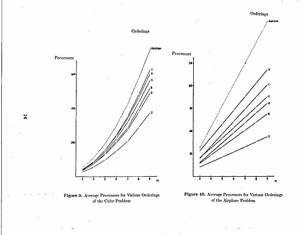
Figure 9. AverageProcessorsfor VariousOrderings Figure 10. AverageProcessorsfor VariousOrderingsof the Cube Problem of the AirplaneProblem
orderings. For the cube problem, 200 random orderings were examined; for the
airplane problem, 100. Average results from this testing are listed in Table 5 and
plotted in Figures 7, 8, 9, and 10.t-
"° Table 5. AverageComplexitiesfrom Random Orderings
Cube Problem Airplane Problem
Total time steps: 102.72n 2 + O(n) 256.04n + O(1)
Maximum processors: 21.96n 2 + O(n) 50.63n + O(1)
Averageprocessors: 11.67n2 + O(n) 27.58n+ O(1)
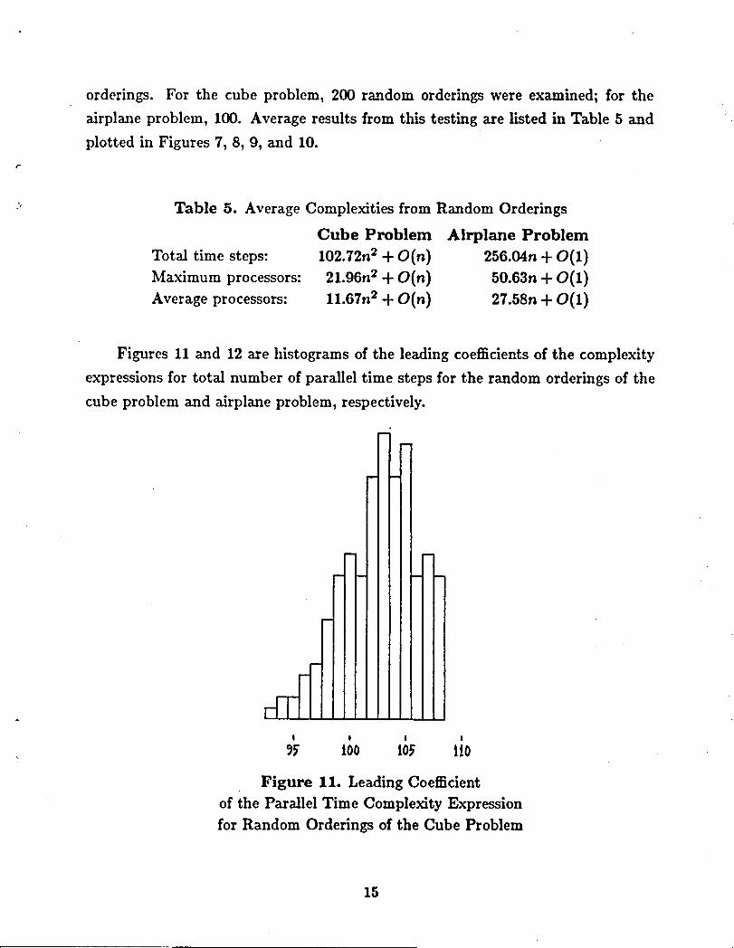
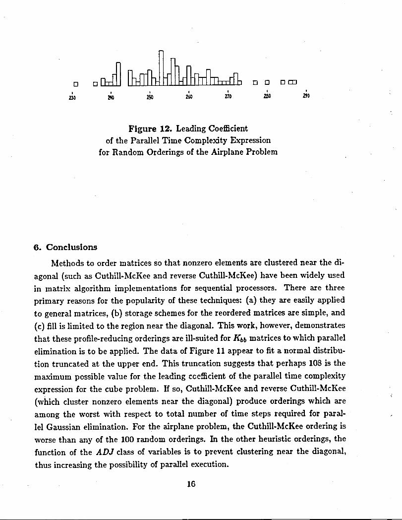
FiguresIIand 12arehistogramsoftheleadingcoefficientsofthecomplexity
expressionsfortotalnumberofparalleltimestepsfortherandomorderingsofthe
cubeproblemand airplaneproblem,respectively.
m
m
m m
m m m
I I I I
_ t00 t05 ti0
Figure 11. Leading Coefficientof the Parallel Time Complexity Expressionfor Random Orderings of the Cube Problem
15
D D_b_ _ [3 D Drn
' ' _0 ' _ Z_0 '23O _q¢ 2 Z60 0 290
Figure 12. Leading Coefficientof the Parallel Time Complexity Expression
for Random Orderings of the Airplane Problem
6. Conclusions
Methodstoordermatricessothatnonzeroelementsareclusterednearthedi-
agonal(suchasCuthill-McKeeandreverseCuthill-McKee)havebeenwidelyused
in matrixalgorithmimplementationsforsequentialprocessors.Therearethree
primaryreasonsforthepopularityofthesetechniques:(a)theyareeasilyapplied
togeneralmatrices,(b)storageschemesforthereorderedmatricesaresimple,and
(c)fillislimitedtotheregionnearthediagonal.Thiswork,however,demonstrates
thattheseprofile-reducingorderingsareill-suitedforKbbmatricestowhichparallel
eliminationistobeapplied.The dataofFigure11appeartofitanormaldistribu-
tiontruncatedattheupperend.Thistruncationsuggeststhatperhaps108isthe
maximum possiblevaluefortheleadingcccfficientoftheparalleltimecomplexity
expressionforthecubeproblem.Ifso,Cuthill-McKeeandreverseCuthill-McKee
(whichclusternonzeroelementsnearthediagonal)produceorderingswhichare
among theworstwithrespectto totalnumber oftimestepsrequiredforparal-
lelGanssianelimination.Fortheairplaneproblem,theCuthill-McKeeorderingis
worsethananyofthe100randomorderings.Intheotherheuristicorderings,the
functionoftheADJ classofvariablesistopreventclusteringnearthediagonal,
thusincreasingthepossibilityofparallelexecution.
16
The attempt to develop heuristics for Kbb matrix orderings for parallel elim-ination appeared to be highly successful. Reordering the boundary node subsetssignificantly reduced the required number of parallel time steps. The best orderingsfor the cube required slightly more than one-half of the time steps required by theCuthill-McKee ordering. For the airplane, time step results from the best orderings
were approximately one-third of the Cuthill-McKee values. Similar results hold ifcomparison is made with average random orderings. Orderings which produced thebest results with respect to total number of time steps were those which minimizedDEG2 as the variable of primary importance, i.e., variations of the minimum de-gree algorithm. Additional work is needed, however, to establish which tie-breakingrules are best. For example, the superior performance of ordering 8 over both or-derings 9 and 10 in the airplane problem is unexpected, since ordering 8 simplyuses ordering 0, rather than ADJ variables, to break ties.
Maximum processor data and average processor data appear to be closely (butnot perfectly) correlated. The average number of processors used per time step isprobably a more important measure of an ordering than the maximum number ofprocessors used during any one time step. The reason for this is as follows. If themaximum required number of processors is not available, some work which could
be performed at a particular time step will not be. However, that work which isperformed will likely produce more work for the next time step. Consequently_ thework to be performed at any given time could consist of both deferred work andnewly available work. It appears, therefore, that if slightly more than the averageprocessor requirement were available, total parallel time step values would not beadversely affected to any great extent. Further studies in which the number of
processors is limited are needed to substantiate this conjecture.
Acknowledgement.
The author wishes to thank Loyce Adams and Merrell Patrick for helpful con-versations which initiated this work, and Larry Dowdy and Steve Schach for theirmany useful comments after careful readings of preliminary drafts of this paper.
17
References
[11L.M.Adams and R.Voigt,"A methodologyforexploitingparxllelisminthefinite element process," Proceedings of the NATO Workshop on High Speed
Computations, edited by J. Kowallk, NATO ASI Serles, Series F 7, Springer-
Verlag, Berlin, 373-392. _-
[2] E. Cuthill and J. McKee, "Reducing the bandwidth of sparse symmetric matri-ces," Proc. 24th Nat. Conf. Assoc. Comput. Mach., ACM Publications (1909),157-172.
[3] A. George, "Computer implementation of the finite element method," Tech.Rept. STAN-CS-208, Stanford University (1971).
[4] A. George and J. W. Liu, Computer Solution of Large Sparse Positive DefiniteSystems, Prentice-Hall, Englewood Cliffs, NJ (1981).
[5] M. R. Leuze and L. V. Saxton, "On minimum parallel computing times forGanssian elimination," Congressus Numerantium 40 (1983), 169--179.
[6] A. Noor, H. Kamel, and R. Fulton, "Substructuring techniques--status andprojections," Computers and Structures 8 (1978), 621-632.
[7] G. Strang and G. Fix, An Analysis of the Finite Element Method, Prentice-Hall, Englewood Cliffs, NJ (1973).
[8] W. F, Tinney, "Comments on using sparsity techniques for power system prob-lems," Sparse Matrix Proceedings, IBM Research Rept. RAI 3-12-69 (1969).
18


I ReportNo. NASA CR-172466 2. Government Acc,,,,,ion No. 3. Rec;pi,nt*s C_Iog No.
ICASE Report No. 84-474. Titleand Subtitle 5. Report Date
Parallel Triangularization of Substructured Finite September 1984
Element Problems 6 PerformingOrganizationCode
7. Author(s) 8. PerformingOrgan;zation'Relx_rtNo.
Michael R. Leuze 84-47
"10.WorkUnit No.9. Performing Organization Name and Addre_
Institutefor ComputerApplicationsin Scienceand Engineering 11. Contractor Grant No.
Mall Stop 132C, NASA LangleyResearch Center NASI-17130
Hampton, VA 23665 13. Typeof ReportandPeriodCovered12. Sponsoring Agency Name and Address
Contractor Report
National Aeronautics and Space Administration 14. SponsoringAgehcvCodeWashington, D.C. 20546 505-31-83-01
15. Supplementary Notes
Langley Technical Monitor: J. C. South, Jr.
Final Report
16. Abstract
Much of the computational effort of the finite element process involves the
solution of a system of linear equations. The coefficient matrix of this system,
known as the global stiffness matrix, is symmetric, positive definite, and generally
sparse. An important technique for reducing the time required to solve this systemis substructurlng or matrix partitioning. Substructuring is based on the idea of
dividing a structure into pieces, each of which can then be analyzed relativelyindependently. As a result of this division, each point in the finite element
discretization is either interior to a substructure or on a boundary betweensubstructures. Contributions to the globa! stiffness matrix from connections between
boundary points form the Kbb matrix. This paper focuses on the triangu!arization of
a general Kbb matrix on a parallel machine.
17. Key Words (Suggested by Author(s)) 18. Distribution Statement
parallel computing 61 - Computer Programming & Softwarefinite element method
substructuringUnclassified - Unlimited
19. Security _a_if. (of this report) 20. S_uritv Cla_if. (of this _) 21. No. of Pages 22. Dice
Unclassified Unclassified 19 A02
.-30s ForsalebytheNationalTechnicalInformationService.Sp,nsfield.V,£inia22161


![ICASE REPORT NO. ICASE - NASA · ICASE REPORT NO. 87-24 ICASE SINGULAR ... partial differential equation (e.g., ... Williams [19]. To describe the results in this classic paper, consider](https://img.pdfslide.us/doc/110x75/5af2ff227f8b9ac2469167ce/icase-report-no-icase-nasa-report-no-87-24-icase-singular-partial-differential.jpg)


![NASA Contractor Report 195070 ICASE Report No. 95-27 … NASA Contractor Report 195070 ICASE Report No. 95-27 ... 5.1 The Zonal Fine Grid Scheme 50 ... 15, 16, 17]. Thus, the essential](https://img.pdfslide.us/doc/110x75/5abcbd497f8b9a76038e424d/nasa-contractor-report-195070-icase-report-no-95-27-contractor-report-195070.jpg)