Embed Size (px)
Citation preview

NASA/CR-2002-211449
ICASE Report No. 2002-1
Uncertainty Analysis for Fluid Mechanics with
Applications
Robert W. Waiters
Virginia Polytechnic Institute and State Universi_, Blacksburg, Virginia
Luc Huyse
Southwest Research Institute, San Antonio, Texas
February 2002

The NASA STI Program Office... in Profile
Since its founding, NASA has been dedicated
to the advancement of aeronautics and spacescience. The NASA Scientific and Technical
Information (STI) Program Office plays a key
part in helping NASA maintain this
important role.
The NASA STI Program Office is operated by
Langley Research Center, the lead center forNASA's scientific and technical information.
The NASA STI Program Office providesaccess to the NASA STI Database, the
largest collection of aeronautical and space
science STI in the world. The Program Officeis also NASA's institutional mechanism for
disseminating the results of its research and
development activities. These results are
published by NASA in the NASA STI Report
Series, which includes the following report
types:
TECHNICAL PUBLICATION. Reports. of
completed research or a major significant
phase of research that present the results
of NASA programs and include extensive
data or theoretical analysis. Includes
compilations of significant scientific andtechnical data and information deemed
to be of continuing reference value. NASA's
counterpart of peer-reviewed formal
professional papers, but having less
stringent limitations on manuscript
length and extent of graphic
presentations.
• TECHNICAL MEMORANDUM.
Scientific and technical findings that are
preliminary or of specialized interest,
e._.,o quick release reports, working
papers, and bibliographies that containminimal annotation. Does not contain
extensive analysis.
• CONTRACTOR REPORT. Scientific and
technical findings by NASA-sponsored
contractors and grantees.
CONFERENCE PUBLICATIONS.
Collected papers from scientific and
technical conferences, symposia,
seminars, or other meetings sponsored or
cosponsored by NASA.
SPECIAL PUBLICATION. Scientific.
technical, or historical information from
NASA programs, projects, and missions,
often concerned with subjects having
substantial public interest.
TECHNICAL TRANSLATION. English-
language translations of foreign scientific
and technical material pertinent toNASA's mission.
Specialized services that complement the
STI Prograrn Office's diverse offerings include
creating custom thesauri, building customized
data bases, organizing and publishing
research results ... even providing videos.
For more information about the NASA STI
Program Office, see the following:
• Access the NASA STI Program Home
Page at http://www.sti.nasa.gov
• Email your question via the Internet to
help@ sti.nasa.gov
• Fax 3,our question to the NASA STI
Help Desk at (301 ) 621-0134
• Telephone the NASA STI Help Desk at
(301) 621-0390
Write to:
NASA STI Help Desk
NASA Center for AeroSpace Information7121 Standard Drive
Hanover, MD 21076-1320

NASA/CR-2002-211449
ICASE Report No. 2002-1
* ===========================V
Uncertainty Analysis for Fluid Mechanics with-
Applications
Robert W. Waiters
Virginia Polytechnic Institute and State Universi_, Blacksburg, Virginia
Luc Huyse
Southwest Research Institute, San Antonio, Texas
ICASE
NASA Langley Research Center
Hampton, Virginia
Operated by Universities Space Research Association
February 2002

Available from the following:
NASA Center for AeroSpace Information (CASi)
7121 Standard Drive
Hanover. MD 21076-1320
(301) 621-0390
National Technical Information Service (NTIS)
5285 Port Royal Road
Springfield. VA 22161-2171
(703) 487-4650

UNCERTAINTY ANALYSIS FOR FLUID MECHANICS WITH APPLICATIONS
ROBERT W. WALTERS* AND LUC HUYSE t
Abstract. This paper reviews uncertainty analysis methods and their application to fundamental
problems in fluid dynamics. Probabilistic (Monte-Carlo, Moment methods, Polynomial Chaos) and non-
probabilistic methods (Interval Analysis, Propagation of error using sensitivity derivatives) are described
and implemented. Results are presented tbr a model convection equation with a source term, a model
non-linear convection-diffusion equation; supersonic flow over wedges, expansion corners, and an airfbil: and
two-dilnensional laminar boundary layer flow.
Key words, stochastic, probabilistic, uncertainty, error
Subject classification. Applied and Numerical Mathematics
1. Introduction and Motivation. In the past few years, there has been mnnerous papers appearing
in the Computational Fhfid Dynamics (CFD) literature addressing the subject of credible CFD simulations
(see [1], [2], [6], [7], [10], [21], [30], [33], [351, [36], [38], [39], [41], [42], [49]). In fact, the May 1998 issue of
the AIAA Journal devoted a special section on the topic. Among the key issues discussed in that section
were: Code Verification, Code Validation, Certification and Sources of Uncertainty. One of the primary
reasons for the increased interest in uncertainty management is its application in risk-based design methods.
The structures community and dynamics and controls discipline have a long history :in uncertainty analysis
whereas the computational fluid dynmnics community is a newcomer in this area due in part, to the relative
infancy of the discipline and in part to the large cost, of CFD simulations. However, with the increase in
computing power and software improvements over the past two decades, stochastic CFD is coming of age.
Consequently, the primary purpose of this paper is to serve as an introductory guide for engineers with an
interest in fluid dynamics applications of uncertainty analysis methods.
Befbre proceeding to review the basic methods, some discussion on nomenclature is warranted. In this
paper we adopt the AIAA definitions fbr error and uncertainty [3], namely:
DEFINITION 1.1. E'r'ro'r: A recognizable deficierzcy i77, a_zy phase o7" activity o.f" 'rn, odelirz9 a_zd si77zv, latioT_,
that is not due to lack o.f knowle@e.
DEFINITION 1.2. Uncertainty: A potential deficiency in any phase or activity of the modeling process
that is d'ue to lack of knowledge.
These definitions recognize the deterministic nature of error and the stochastic nature of uncertainty.
Uncertainty can be further categorized into aleatoric (or inherent uncertainty) and epistemic (or model)
uncertainty. Further categorizations are possible and discussed in [29]. This report focuses on methods
for describing and propagating parameter uncertainty in models. In a companion report [29], we describe
methods for dealing with model form and boundary condition uncertainty for the non-linear Burgers equation.
*Virginia. P(_13'techl_ic Institute and Sta|:c Ulfivcrsity, Del)artm(mt of Aerosl)a.(:e and O(:eml Engineering, Bla.cksl)ulg, V'A
24()61-()203 (elna.il: walt('.rs((2_m(m.vt.cdu). This research was SUl)l)orted 1)y tile National A(nOlmuti(:s and Space A(lministra.ti,m
under NASA Colltra.(.:t No. NAS1-971)46 while the. a uth()r was in r(;sidc.n(:e at ICASE, NASA Langley I_.eseal(:h Center, Ha.ml)t(m_
VA 23681-2199.
*S(mthwest R(:sear(:h Institute, P,,(,,lial_ility and Engineering M,;(:lmni(:s: San Ant.(mi(_, TX 78228 (email: llmyse((rswri.e_lll).
This r(_s0.a.r(:h was SUl)l)(_rte(l by the National Aer(mauti(:s ;tll(l Sl)_l(;c Administrati_m ,re(let NASA Colltl';i.(;t N(_. NAS1-97()4(i
whih: the author was in residen(:c a.t ICASE, NASA La.ngley R(:searcll (',elltel, Haml)t(m, \:A 23681-21!0!).
TABLF 1.1
5'o,,.'rce of U',.cc'rt,.i',,.t' 0 a.',M E',r',,'," i',,. CFD Sim',d, ti,,_, ...... s',,.',,.'m.,'ri:_,d .fwm OIw.'rk,,.,,pf and B/,,tt,,.,",'. R,:f. /:¢5]
SollrCC
Physical Modeling
(Assumptions in the PDE)
Auxiliar'.v Physical ModeL_"
Boundary Conditions
Discretization & Solution
Examples
Inviscid Flow
Viscous Flow
Incompressible Flow
Chemically R,eacting Gas
Transitional/Turbuleltt Flow
Equation of State
Thermodynamic properties
"lTi'ansport properties
Chemical models, reactions, and rates
Turbulence model
\Vail, e.g. rougtmess
Open, e.g. far-field
Fret Surface
Geometry Representation
Truncation error- spatial and temporal
Iterative convergence - steady state
Iterative convergence - time dependent
Geometry Representation
Round-Off Error Finit,e- precision arithmetic
Programming &: User Error
In some instances in this report, we have used a more genera] definition of uncertaillty that. ilmludes error
where it is clear t.hat no ambiguity arises.
In the AIAA special issue; Oberkalnpf and Blottner [36] group sources of uncertainty and error arising
from the simulation of physical phenomena goverr_ed by PDE's into four broad categories:
1. Physical modeling
2. Discretization and solution errors
3. Computer round-off error
4. Programming errors
An examination of Table 1.1 shows that many sources of error and uncert.ainty arise in CFD simulations.
It is generally believed that discretization error, geometric uncertainty and turbulence model uncertainty are
the largest, sources of uncertainty in modern t_eynolds-Averaged Navier-Stokes simulations and collectively
account for much of the scatt.er observed between experimental and computational data [2]. Discret.ization
error has been studied extensively and a number of' techniques have been proposed t'or modeling this error
(see e.g. [40], [41], [43]). Grid adaptation schemes frequently use these models tbr improving the base
grid. The impact of geometric uncertainty has been st.udied 1:)3:Darmofal [13] tbr compressor blades ltsing
probabilistic methods. Although relatively little has been done tbr quantifying turbulence model uncertainty,
there has been some work in this area [8], [20]. More recently, Godfrey [19] used the continuous sensitivity
equation approach to rank the relative importance of the closme coefficients in three turbulence models:
theBaldwin-Lomaxalgebraicmodel,theSpalart-Alhnarasone-equationmodelandthe\¥ilcoxtwo-equationk - co turbulence model.
With the present state of computational resources, some sources of error can be made negligible. For
example, for essentially all one- and two-dimensional steady, inviscid or laminar flows, a user typically has
sufficient hardware to drive the discretization error to very low levels, essentially zero, leaving model un-
certainty as the only significant source of uncertainty. Over time, this trend will continue and eventually
encompass a large class of three-dimensional sinmlations. However, without further research effort concen-
trated on uncertainty estimation and managernent, model uncertainty will likely remain relatively constant
over time since it is not a known error that can simply be reduced with additional computing power.
In the next section, we review methods that can be used in CFD simulations for dealing with error and
uncertainty. Next, a range of problems starting with some simple model problems and ending with laminar
boundary layer flow are presented.
2. Review of Uncertainty Analysis Methods. In this section, we briefly review deterministic and
probabilistic methods for uncertainty analysis. Two deterministic uncertainty analysis methods - 1) Interval
Analysis and 2) Propagation of error using sensitivity derivatives and three probabilistic methods 1) Monte
Carlo, 2) Moment methods, and 3) Polynomial Chaos are summarized below.
2.1. Interval Analysis. The basic idea in interval analysis is to perform operations on input intervals
that contain the set of all possible values of the input in such a way that the output interval consists of all
possible values of the result of the operations performed on the input. Consequently, interval results represent
maximal error bounds (i.e., worst case results). One of the most appealing things about Interval Analysis
(IA) is that it can be implemented in a systematic way on modern computing systems such that the details
of the interval operations are transparent to the user. Thus, one can take an existing simulation tool, such as
a CFD code, and immediately implement interval analysis provided that it is supported by the programming
environment. However, it should be pointed out that different expressions for computing an interval output
quantity can result in different interval widths even if the expressions are mathenmtically equivalent for
pointwise input. To demonstrate this, consider the following two expressions that are equivalent for point
values,
m 1-- and g(:c) -- I "(2.1) f(:c) 1 + Z 1 +-
2C
Table 2.1 shows the results of performing interval analysis for these two functions for input intervals, at,
defined in terms of the interval midpoint value, T, and uncertainty, c, by
(2.2) z = ¥[1 - s, 1 + e].
Values in the table correspond to e = 1/10. Note that the interval width associated with the second relation,
9(z), is substantially smaller than the width found by evaluation of f(z). This shows that, although existing
software can take immediate advantage of interval analysis, siglfificant improvement in the size of the error
bounds may be possible by careful design and construction of the operations within the software. However,
this investment may not be prudent since probabilistic methods provide much more information than can
be obtained through interval analysis. This exmnple also illustrates one other point: the fact that different
interval results can be obtained is not related to the precision of the calculation. Here:. rational numbers were
used to carry out the operations exactly. Different interval output occurs because sel; theoretical operations
- union, intersection, complement are affected 1)3"the st,ructural .[bT'm of the operations.

TABLE 2.1
l'll l e'r ml l a.'lm.l!l._i._ 'r_:._"u.lt._ .[o'r tu;o ._i'm plc c:rlrr<_.',.'ri<m..'_ t lm.l a.'r<; _qu.imdc'/_.l .[o'v ])_ri'lp.t _.,o.lu< ._ b td 'tm l .[,'r ilp f _:m,o l._.
x11] , 11 "T6 7 '7
5
.q 9
7 ,,5-6 i-7 T7
2 "T _
f(x) g(x)
:_ _ I
7"7t 103' _]
[5;"] [5
3
9 ] 1 7,_ 7
4
Moreover, interval arithlnetic inside iteration loops results in error growth each iteration without sortie
modification to the base algorithm (see Sect.ion 3). Since many fluid dynamics codes rely on iteration for the
solution process, this further detracts fl'om the use of this approach. In a probabilistic modeling, varying
degrees of correlation between random variables can readily be taken into account in the anahsis. The
practical examples of Section 5.2 and 6.2 will illustrate this point and indicate that, depending on the
value of the correlation, the uncertainty may be larger or smaller than in the case where all \-ariables are
independent. Since interval analysis is a deterministic rnethod, it cannot take advantage of this informatioll
and nlust necessarily compute the widest bounds.
2.2. Propagation of Error using Sensitivity Derivatives. Error propagat.ion using sensitivity
derivatives has been in use for man 5, years (see e.g• Dahlquist and Bjorck [9]) If ,, = t,.({, c ) where c• , .... %`,, %.i
is the i t_' indeI:)endent variable with error A_i associated with it. then a deterlninistic approximation to the
error, A'u, is given by
I
(2.3) A_, _ _ A_!,i2 .L¢= 1 0 %.i i
A computat.ional fluid dynamics example of' this technique is presented in the work of Turgeon et. al., [11], in
which the laminar flow of corn syrup was analyzed subject to uncertainty in the viscosity model, the thermal
conductivity model, the geometry, and t.he boundary conditions. In their work, they used the continuous
sensitivity ......equation method (see Section 4) to evahmte the sensitivity derivatives, eTZ,.,°"in Eq.(2.3). This
results in an error estimate, At,, which in their work was shown to bound the experimental data. \,_,_ wish
to emphasize that this approach is based on the assumption that a particular input interval (for example;
one of their inputs was an experimentally measured temperature, T 4-2(_), contains the e'nti're uncertainty
interval due to this variable. We will contrast this with a probabilistic framework in Section 2.4.
2.3. Monte Carlo. Although there are many different applications of Monte Carlo simulation, both
deterministic and probabilistic, the tbcus in this report, is on probabilistic sinmlation methods. A briefly
history of the method is given by Hammersley and Handsco:mb in [241 and summarized here. Arguably;
the development of the method and name. Monte Carlo, is considered to have its start around 1944 when
yon Neumann and Ulam performed direct simulation of neutron transport problems, primarily as a tool for
atonfic bomb research• Shortly after the end of \Vorld \_;ar II, Fermi, Ulam, ,,;on Neumann and others began
applying Monte Carlo methods to deternfinist.ic woblems. By 1948, Monte Carlo estiinates of the eigeiwalues
of the SchrOdinger equation had been obtained. Sometime thereafter, this work came to the attention of Dr.
Stephen Brush at the Livermore Laboratory who subsequently unearthed a 1901 paper t)3 Lord Kelvin [31]
in which remarkably modern Monte Carlo techniques appear in connection with the Boltzmann equation.
80
60
40
20
i000 samples350300250200150i0050
0.2 0.25 0.3
I0000 samples
....
0.2 0.25 0.3
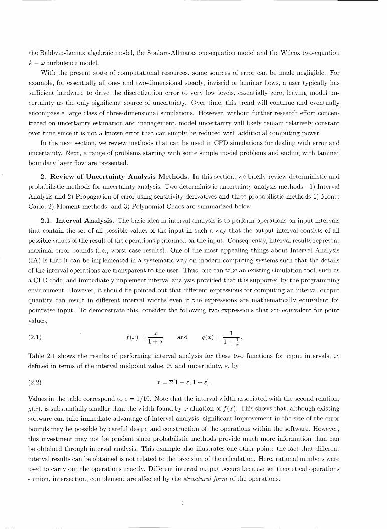
FIC:. °.I. T!Ipicalh.istog'ra,'m,._obt.a.i',,edby .sa.'m,pli',,g.fro'm,o, No,r,m,,,ldLs'l'ribt't/.lio'n,,wilh,a 're,ca'n, of (1.25 a.'nd_I_.stw/l.dwrddcviat'io'l_,of 0.025co'r'rc.>'po',.di',,.qto ,, coc./.]i.cic',,tof _a.ri,.tio',,.CoV = 10%. L_.:.fl- J.l)Ol)._rm.l,l___,i_i.qh.t10,01]0._a.m.ph._.
Apparently, the methods were obvious to Lord Kelvin and consequently his focus was on the results. Even
prior to this application, there are isolated accounts of the method [23].
Here we demonstrate one of the simplest of all Monte Carlo methods, referred to as crude (or basic)
Monte Carlo. In this approach, the basic procedure is:
1. sample input random variable(s) from their known or assumed (.joint-) probability density function
2. compute deterministic output for each sampled input value(s)
3. determine statistics of the output distribution, e.g., mean, variance, skewness, ...
The statistics of a distribution (mean, variance, skewness, kurtosis, ...) can be determined from the
definition of the expected value of a function of a random variable, _, say g((), name,15_
/c c c C(2.4) =
where p(_) is the probability density function of the distribution that describes some event or process and
the integration is over the support of the PDF. The mean of the probability distribution (also referred to as
the first moment about the origin) is
/(2.5) = =
The r th moment about the mean is given by
'(_- ,,) p(_.)d_.(2.6) IE[(_-_)"] = -E," c
The variance, skewness, and kurtosis are related to the 2"d, 3_d, and 4th moments about the mean. In
some cases, the integrals can be evaluated analytically, in others, the integrals are replaced by discrete sums.
In the application problems to follow, we sampled fi'om a Normal (Gaussian) distribution with a mean #
and standard deviation c_. The probability density function (PDF) of the Normal distribution, PN(_), also
denoted N[#, c_], is given by:
C 2o.2
(2.7) pN( ) -
Two typical samples are shown in Figure 2.1 in which the Gaussian shape of the underlying PDF is evident.
Frequently, it is convenient to use the standard normal variable. N[0, 1], i.e., a Gaussian with a mean of 0
and a variance of 1. it,s definition follows directly fi'om Eq. (2.7).
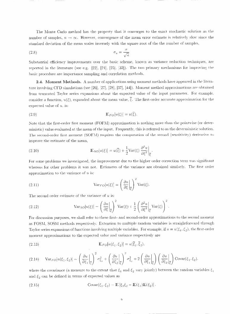
Tile Monte Carlo method has the property that it. converges to the exact stochastic solution as the
number of samples, n --+ oc. However, convergence of the mean error estilnate is relatively slow since tile
standard deviation of the mean scales inversely with the square root, of the t,he rmmber of samples:
(7
(2.8) c7,,= _,
Subst, antial ef[icienc3; improvement, s over the basic scheme, known as variance reduction techniques: are
reported in the literature (see e.g. [22]: [24]. [25]. [32]). The two primary nlechanisms for improving the
basic procedure are importance sampling and correlation methods.
2.4. Moment Methods. A number of" applications using moment methods have appeared in the litera-
ture involving CFD simulations (see [26]: [27], [28]: [37]. [44]). Moment method approximations are obtained
fl'om truncated Taylor series expansions about the expected value of the input parameter. For example.
consider a function, u(_). expanded about the mean value, 4. The first-order accurate approximation for the
expected value of u. is:
(2.9) _Fo[_,(_)] = _,(_).
N-ot.e that the first-order first moment (FOFM) apl)roximation is nothing more than the t)ointwise (or deter-
ministic) value evaluated at the mean of t.he input. Frequently, this is referred to as the deterministic solution.
The second-order first, moment (S()F_[) requires t.he computation of the second (sensitivit.3') derivative, t.o
improve the estimat, e of the mean.
1 O2'u(2.10) Es'o['u.(_)] = ",.(_) + __Var(._) 0--7 .
For some problems we investigated, the iml)rovement due to the higher order correction terrn was significant
whereas tbr other problems it was not. Estimates of the variance are obtained similarly. The first order
approximation to the variance of 'u is:
9
( )-c)_ "v_r(_).(2.11) VarFo[u(#)] = 0--_ 7
The second order estimate of" the variance ofu is:
2 )'2(2.12) Varso[_,,(_)] = a_,, Wr(_) + -- V_r(_)
• . _ _ O_2&- _
For discussion purposes, we shall refer to these first.- and second-order approximations to the second moment
as FOSM: SOSM methods respectively. E.xtension to mult.iple random variables is straightfbrward throughc
Taylor series expansions of functions involving nmltiple variables. For example, if i_,= "_z(<{l, s2). the first-order
moment approximat, ions to the expected value and variance respectively are
c c(2.is) n; ro [,,(_ ,.._,)]= _(_. __).
. ( )( )(914) VarFo[U(_lc-. •s.,)] = _ )__ ere, W -- rr_ + O -- Covar(<l _'))- &.j _- #)G g
where the covariance (a measure to the extent that sc] and _2cvary., .jointly)., between the random variables _1
and _2 can be defined in terms of expected values as
c c c(2.15) Covar((,, <.-2) IF, [,,_,2 - IE((,)E(_2)] •
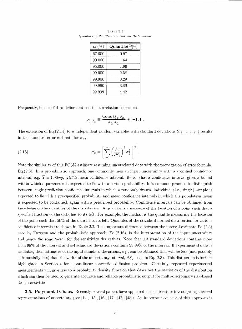
TABLE 2.2
Q,.,a.'n,t.i,h_._ o.f th, e Sta,_ut.,'rd No'rm..l Dist'ri, bu, tion.
c_ (%) Quantile(_)
67.000 0.97
90.000 1.64
95.000 1.96
99.000 2.58
99.900 3.29
99.990
99.999
3.89
4.42
Frequently, it is useful to define and use the correlation coefficient,
__ Covar(_l, _2)C [-1, 1].
P_ ,_ -- cry, cr_
The extension of Eq.(2.14) to n independent random variables with standard deviations (cry,, ..., cry,, ) results
in the standard error estinmte for cr_....
I
(2.16) or,, = _., .ki=l
Note the similarity of this FOSM estimate assuming uncorrelated data with the propagation of error formula,
Eq.(2.3). In a probabilistic approach, one commonly uses an input uncertainty with a specified confidence
interval, e.g. T ± 1.96c, T, a 95% mean confidence interval. Recall that a confidence interval gives a bound
within which a parmneter is expected to lie with a certain probability. It is common practice to distinguish
between single prediction confidence intervals in which a randomly- drawn, individual (i.e., single) smnple is
expected to lie with a pre-specified probability and mean confidence intervals in which the population mean
is expected to be contained, again with a prescribed probability. Confidence intervals can be obtained fl'om
knowledge of the quantiles of tim distribution. A quantile is a measure of the location of a point such that a
specified fraction of the data lies to its left,. For example, the median is the quantile measuring the location
of the point such that 50% of the data lie to its left. Quantiles of the standard normal distribution for various
confidence intervals are shown in Table 2.2. The important difference between the interval estimate Eq. (2.;3)
used by Turgeon and the probabilistic approach, Eq.(2.16), is the interpretation of the input uncertainty
and hence t,he scale .fi_ctor for the sensitivity derivatives. Note that -t-3 standard deviations contains more
than 99% of the interval and -+-4 standard deviations contains 99.99% of the interval. If experimental data is
available, then estimates of the input, standard deviations, cr_, can be obtained that will be less (and possibly
substantially less) than the width of the uncertainty interval, A(_,, used in Eq.(2.3). This distinction is further
highlighted in Section 4 for a non-linear convection-diffusion problem. Certainly, repeated experimental
measurements will give rise to a probability density function that describes the statistics of the distribution
which can then be used to generate accurate and reliable probabilistic output for multi-disciplinary risk-based
design activities.
2.5. Polynomial Chaos. Recently, several papers have appeared in the literature investigating spectral
representations of uncertainty (see [14], [15], [16], [17], [47], [48]). An important concept of this approach is

thedecompositionofarandomfunction(o1"variable)int,oseparabledeterministicandstochast,iccomponents.Specifically.foravelocityfieldwith rarlclomfluctuations,wewrite.
P
i=0
where tLi.(;r) is tile deterministic part and g2i(_) is the random basis function corresl)onding to the i th mode.
Effectively, _i(:c) is the amplitude of the i Lh fluctuation. The discrete sum is taken over the number of
modes represented. P - (n,+_,)! which is a function of the order of the polynomial chaos, l)- and the number
of random dimensions..n. Here, we use nmlt.i-dilnensional Hermite polynomial basis functions to span the
n-dimensional random space that_ we wish to 1"el)resent. akhough the use of many other basis functions are
possible. A convenient fbrm of the Hermite polynomials is given by
e"'_ (-1)" --e :(2.18) H,,({i,, ..-._,i,,) = e_, 0" --' e"e• . . 0<,i,,8_,i ' '- c
where ( = (_,:, : ..., s,i,, ) is the n-dimensional random variable vector. As discussed in [47], there is a one-to-one
H c ccorrespondence between the functions ,_(si ) and k_i(_i). The Hernfite polynomials torln a complete1 t .... _ ,_,, . ,_
orthogonal set. of basis functions in t,he random space. In terms of the inner product.,
(2.19) (fc(_,)f_/(s),c\= .f (s).q (s) I"1';(_)d_'c c, C'_'
with the weight functio11 I¥(_) taking t.he form of an 'n.-dimensional Gaussian distribut.ion with unit variance
defined 1)3;
1 __, _,_(2.20) l,I,"(_) - _e -'" "
Vs(.2rr) ''
t,he inner product, of the basis functions is zero with respect to each other, i.e..
(2.21) (q2i_9.i) = < _9) (q-,"ij.
where 6Li is t.he I(ronecker delta funct.ion. Once t.he modes, v,a., of the solution are known, then statistics
of' t.he distribution can be readily evaluat, ed. The mean of the random solution is given by IEpc,['u] = uo.
The _: = 1 ..... 'n, rhodes are the Gaussian estimates of the variance, all higher modes provide non-Gaussian
int.eractions. The variance of" the distribution is given 1)5
P
(2.2_o) = Ei.=l
3. Linear Convection with a Source Term. The prilnary focus of' this example is on the apl)lication
of int.erval analysis for both time-dependent and steady-state calculations. \Ve consider the scalar wave
equation with a source term designed to mimic chemically-react.ing flow problems in which T plays the role
of a chemical time scale• 7- + l//cf, where l_:f is the fbrward reaction rat, e. The governing equation is
(3.1) /)t _ o &,: 7,
in which o is the com;ective wave speed (taken t.o be o = 1 tor all cases considered). Near chemical
equilibrium, reaction rates are essent.ially inst.antaneous, i.e., l,:f + .:_ and 7- _ 0. restflt.ing in disparate
time scales that cause numerical ::stiffness". This problem has been studied 1)y Godfrey [18] in connect.ion

O2
11
U
0
1
with implicit preconditioning algorithms. Here, we consider uncertainty in the chemical time scale, 7, due
t,o uncertainty in measured reaction rates. The exact solution to this equation is
:': r)e-xl_.(3._9.) _(., t): V(t- -,O,
In order to complete the definition of this problem, the initial and boundary cond.ition, respectively, are
taken to be
(3.3) u(x, 0) = 1 :c C [0, 1],
(3.4) _L(0, t) = 1 V t > 0.
With these conditions, the function, 9, is
x r)=( 1. t> :±(3.5) 9(t - a" e -(t-'_/_)/_ 0 < t < _-:
• -- o"
Taking the chemical time scale, r = 0.9, and the wave speed, a = 1, a graph of the exact deterministic
time-dependent solution from t = 0 to t = 1 is shown in Figure 3.1. For the uncertainty analysis, we will
examine the time-dependent behavior at z = 1 (seen along the front side) and the steady state solution (seen
along the right edge).
3.1. Interval Analysis. First-order upwind differences were used to approximate the spatial derivative
in Eq. (3.1). The outflow boundary condition (:c = 1) was prescribed by approximating &' = 0 to first- _ z--1
order accuracy. Three time integration methods were implemented: Euler explicit, Euler implicit, and 4-
stage Runge-Kutta. In terms of the steady-state residual. R(u) - a°" ,u, T/z + 7, the Euler explicit method for
ut + R(u) = 0 can be written as:
(3.6) ,L(n+_) = 'tt ('_) - AtR(_t ('')) (Euler Explicit-I).
For a deterministic problem, that is all there is to this method (referred to hereafter as Euler Explicit - 1).
However, consider the case in which there is uncertainty in the input chemical time scale, r. Let r be defined
to be the interval
(3.7) r = _[1 - c. 1 + c],
where _ is the midpoint of the interval with uncertainty a. The residual in Eq.(3.6) is now arl interval rather
than a point value at any x location. Moreover, v.(') is also an interval after the first iteration as a consequence
of interval operations during the previous time step even if the initial condition has no uncertainty. As seen
in Figure 3.2. this method results in exponential g_'owth of the intervals during a time accurate simulation.
One can consider alternatives, namely.
(3.8) 2Z('n-l) = ZL('') -- AtR(-g ('')) (Euler Explicit-2)
(3.9) ,l/(,zq-1) = 77(,,) _ AtR(u(',,)) (Euler Explicit-3)
(13.10) v,(''+_) = 77('') - AtR(_/'_)) (Euler Explicit-4).
where E is the midpoint of the interval. Methods 2 and 4 evaluate the residual with the midpoint of' the
interval from t.he previous time step. However, R('E ('')) is still an interval since the chenfical time scale
is uncertain. Since Method 4 also uses the midpoint value in the time derivative, it gives onh" the local
uncertaint.y at. each step due strictly to the uncertainty in r. For this problem, this results in very small
interval estimates in which the upper and lower interval bounds visually appear t.o be on top of one another.
Method 2 uses the interval "u/") in the time derivative and hence accounts for cumulative growth. In fact; at
any point in time, the cumulative (integrated) stun to time t of the uncertainty from Method 4 is equivalent
to the Method 2 uncertainty at time t. Methods 1 and 3 both use the interval "u.(") to evah.mte the residual
and hence allow fbr teml)oral growt, h of uncertairlty. The magnitude of the outpllt intervals will grow without.
bound in Method 1 and yet with Method 3 converge to steady-state values (provided a steady-state exists).
The results of these four methods with 81 equally-spaced grid points along the ._,- azi,s and using a timea,_l, 1
step At corresponding to I = _:,: = 5, are shown in Figure 3.:2.
It is common practice to monitor the convergence of a solution process in CFD sirmflations in terms of
a vector norm of the steady-state residual, R('_ (')). In this case. however, _(_l. (''/) is an interval not suitable
for obtaining point-wise vector norm values hence we monitored the L2 -'norm of R(77(")). The residual
histories of the tour methods are shown in Figure 3.3. For Method 1. the interval size rapidly reaches the
maximum maclfine representation, on this COlnputer {-1.79769 × 10 a°s, 1.79769 × 10³°s } which results in a
midpoillt residual of zero although t.he solution is completely useless. The other three methods smoothly
converge to the steady-state in t < 2 yet the exact steady-state is achieved at. t = 1. However, in all cases.
the residuals at t = 1 have been reduced more than three orders of magnitude and the values at tiffs time
are close to their steady-state values.
One of the most common 4-stage Runge-I<utta methods (and the one implemented) can be writ.ten as
(3.11)
72 = R("a('') + 7_/2).
Y3 - R(u<'') + 72/2) •
74 = R,(u (") + 7:3).
,'__ku('_) = _ ....-- ("q-,(71 ÷ 272 -- z, i3 -F 74).
u(,,+l) = u(,,) + A_t('').
Again, we face the same issues as before, namely the residual evahmt.ion, R('u) vs R(g). and the update step,
"u,('") vs _('"). Numerical experiments confirm that the use of /_,(7i) fbr the residual evaluations and u,('') in
the update st.ep yields the most useflfl interval analysis results.
For many CFD simulations, implicit time integration met.hods are preferred. For demonstration pur-
1(I

500 - -'
25O - - '
'; i ..... Euler Explicit - 1
, " ,
0.2 03 04 0.5
Time
0.9
08
Euler Explicit - 2
0
°'6I_05
0,3
02 - -- ,,,,,,,,,,,,,,,0 0,5 I 15 2
Time
1 .
0.9 ,
0.8 !
O.7 ,
- i'
= 0,5
04 - +T
0,3
0.2
01
o i )0 0.5 1
Time
Euler Explicit - 3
I I
, _1 +1.5
1
0.9
0.8
0.7
06
05 _"m
o,4
0.3
02
Ol
2 0
-- Euler E'<plicit - 4
\
0.5 1 15 2
Time
FI(;. 3.2. I'n,t,+.."rm+,l+m,a,l'fl.s'L; r_:_._u,lt.s ,,.si,'n.fl d'_t]'_:'r+:'n.!l;+l,r'i++,t'i,_,.s +m, t,h,_ E,,l_?" E:rp/ic'it 'm,+;th,od.
10 2
10o
10 .2
:3
10 4
tv,,_ 10 +0
E__ 10 +0Z
_J_'l01°
1 0 12
1 0 -14
I I
\\
\
Euler Explicit - 1Euler Explicit - 2
Euler Explicit - 3
Euler Explicit - 4
\\\\
Y,
i I i i i r I1 2
Time
FI(;. 3.3. C'+m,t;+_ql(:ll,+:_:h,'],slo'ri_,.'_.fo't" l,h.+:'.four ¢'m,pl_m_,c'n,ta,l'i+m,.,," of l,lm Eu,l+"r E:q, li+',il 'm,+_ttmd .f,r 'i'n,L_,'r,t:+da.'nn,//l.,,"i.,,.
1]
poses, we implemented the Euler implicit time integration scheme which in delta fbrn_ can be written as
1 OR) ('')(3.12) A--t, ÷ &,--
This results in the tri-diagona] set of equations
(3.]3)
bl c1
o.2 b2 c2
0 (In-1 bn 1 C__l
(in /)n
/N?I- 1
A u2
/2(lll)
R,('.,e)
where tbr the general case of wave speeds of either sign,
o j ---- c,+lal2,.,,._. )
1 , 1 , I C'l / .j == 2 ..... "I'1 -- I.
(3.14) bo = _- _- , _:_.o.-I_,1
C.j = 2",:r
At. the inflow boundary: cl = R.('ul) = 0 and bl = 1 and at. the outflow, o,,, = -1, b,,. = 1:/2(u,,) = 0.
For positive wave speeds, the above matrix reduces to a lower hi-diagonal matrix which cart be solved
by a fbrward substitution pass. Likewise, for negative wave speeds, the nmtrix (with appropriate change in
boundary conditions) reduces to an upper hi-diagonal matrix which can be solved 193,a backward substitution
step.
Using the interval midpoint for residual evaluations, a comparisor,_ of' the time history from the Euler
explicit, Euler implicit, and 4-st.age Runge-t(utta methods at. a: 1 is shown in Figure 3.4. Although difficuh
to see. the Euler implicit and Euler explicit, methods yield identical results in terms of interval size. The
Runge-I(utta niet.hod results in larger intervals due to the increased number of residual evahmtions and
intermediate update steps in the nmlti-step method.
If" one is only interested in the steady-state solution, other options become available, prirnarily through
the use of algorithms that are stable for large tirne steps and in some cases, space-marching methods. In this
case• both are applicable. For example, the Euler implicit met, hod, Eq. (3.12) can be used with At -+ >c.
Since the governing equation is linear, the steady solution is obtained in one step 1)3 solving the resulting
linear problem which we refer to as a Time March method. The other alternative is to implement a Space
March method by eliminating the time derivative in Eq. (3.1), i.e.,
(3.1.5) o....()d' T
Discretizing this equation with first-order upwind diffhrences (t, aking o. > O) yields
_u.j_ ](3.16) 11.;-
1 + ,,x._:(1 T
where u.j - _L(3A:r). The results of" the Time March versus Space March approaches can be seen in Figure
3.5 where the advantage of' space nmrching is evident.
12
1
0.9
0.8
0.7
0.6
0.5
0.4
0.3
0.2
0.1
0
0
Euler Explicit....... Euler Implicit.
4 stage Runge-Kutta
0.5 1 1.5 2
Time
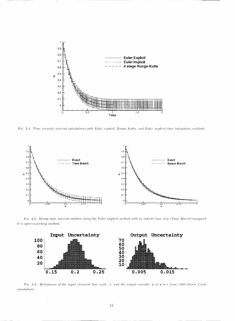
F IC. 3.4. T'i'm,_" _t_;ctl,'nd, c "in,t_'rml.l c_dc'_t, lM,'io'n,,_" mith, Eu, lf::'r c:l:pl'ir:'it; R'tm, fle-I_"u, tl_l,. _m,d £tt, l_l" 'i'm, pl'ic'i/ lim,c 'i'ntcfl'r_H'ion, 'm, eth, od.s.
1
0.9
0.8
0.7
0.6
0.5
0.4
0.3
0.2
0.1
0
o
1
0.9
0.8Exact
0.7
0.6
0.5
0.4
0.3
0.2
0.1
0i F I i I , , , I I , , . T=ta'4-J-4-J-±$ I I I
0.25 0.5 0.75 1
X
Exact
, , = I _ , t , I , , , t I i i , _ I0.25 0.5 0.75 1
X
FtC. 3..5. St, emt'!l ._'t_l.Lc _'H,t <_'rmd sohl, t,'io'n, 'u,._'m, fl t,h,c EM,m" "i'm, pl'ic'it, 'm,c,t,h, od 'mith ,m, "i'n,.fi'l_,'ite _mJ,_:: ,_l_q_ ('T'i'm,e Ma,'n:h,) cO'm lm.'r<'d
1,o _ .s'p_z, cc-'m,(l,'rch,'i'n,!l 'm, cth.od.
100
80
60
4O
20
Input Uncertainty
70605040302010
0.15 0.2 0.25
Output Uncertainty
0.005
FIC. 3.6. H'i._tO!l'ra/m,.s of the ,i'n.p,ttt ch,_;'m,i_;a,l l,im, c ._c_z, le:. 7. a,'n,d l,h,c o,M, pu, l mlriahlc. _z _zl :r : I .[_'_'t_ 1000 Mon, h' Ca,'rlo
,s,m_,_tla, tio,n,,_.
1
0.9
0.8
0.7
0.6
0.5
0.4
0.3
0.2 I0.1
0
-- x=1/10
} x=1/2
_, o Deterministic
_\ -- x= 1
\\ .... 95% Single CI
\ \ .........
_,o ccc _oooo occ coo oo coo _-.o'..;o.c oo_ oo_oooo
__ ". .................
\ \_\ _ _
'_ \X\ &_ .............
\ \
0.25 0.5 0.75 1
Time
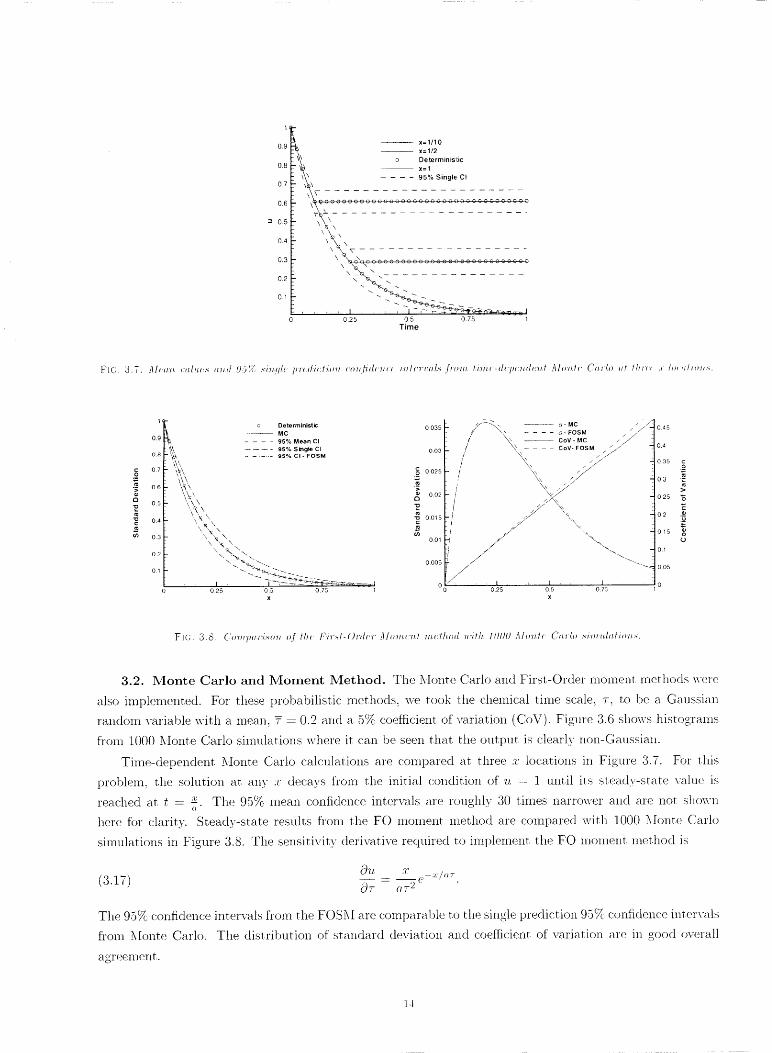
Fie;. 3.7. Ah'u',. _1l,.,._ ,,.d .95'.'_;1._'m.flh"])r(dicl'hm cou./ffdc'uc_ m lcT't_ol.,,'.f'r(,'m li,m.c-dW)c'udc_J.lAlo'n.lc C_lTlo at lhl_ .r h,,tUm._.
0.9
0.8 . :,,_
O. 7 [ \\\!x
0 6 [ "_\\1- 'q,\I- %\
0 5 _\ \ \
'\_, \,
0.4 "\,.4, ', \,
",, ,_ N03
0.2
0.1
c Deterministic
-- MC
- - - 95% Mean CI
.... 95% Single CI
....... 95% CI - FOSM
\ %,"\
-,.)-<.>_
0 25 0.5 0.75 1
x
I ,_"_- _ - a - MC / /-0035. ' ""_,, .... _- FOSM /// 1 045
/_' -- CoY- MC /_// 404I- / "_ - cov-_osM . "/ ":1
0.03 | / _ / _ -I
_oo_ / 4o._5 _
0o,_i //" ... 1o15
-10o O0 0.25 0.5 0.75
x
FIe;. 3.S. Co'mim'vL_o'n of lh+ Fh'._l-()'nh"v Mom.c'Hl "m,cth<m: ,,'/.lh. ld()O Alo'u/c Cu'v/o ._huu./alhm.._.
3.2. Monte Carlo m_d hloment Method. The Monte Carlo and First-Order moment methods were
also implemented. For these probabilistic methods, we took die chemical time scale, r. to be a Gatlssian
random variable with a mean, 7 = 0.2 and a 5% coefficient of' variation (CoV). Figure 3.6 shows histograms
fl'om 1000 Monte Carlo simulations where it. can be seen that t.he output is clearly non-Gaussian.
Time-dependent Monte Carlo calculations are compared at three :z: locations in Figure 3.7. For this
problem, the solution at. any m decays from the initial condition of "u, = 1 until its steady-state value is
reached at, t = ± The 95% mean confidence intervals are roughh' 30 times narrower and are not showno " '
here for clarity. Steady-state results from the FO moment n_.ethod are compared with 1000 kionte Cmlo
simulations in Figure 3.8. The sensitivity derivative required tO implement the FO moment method is
_u. 37 -:r/o.r
(3.17) Or - (,r 2 e
The 95% confictence intervals from the FOSM are comparable to the single prediction 95c/c confidence intervals
fl'om _[onte Carlo. The distribution of standard deviation and coefficient of variation are in good overall
agreement.
0.9 /"" \ "
0.8 /// \_A
0.7 / / _,_
0.6 //./ _ //
-- ',/" 0.5 .... U /I f_'"
O. 4 A/A / / /...... du/dp
0.3 / _A / /
0. ,,, , ....- -2 -I 1 2
1
0.8
0.6
0.4
0.2
=,_"00 "-.
-0.2
-0.4
-0.6
-0.8
-13
4 ....
3
1
0 _
\\
-1
-2
\ I
-3 \ IJ
-4_
-2 -1
d2u/dp 2 ! "_
d3u/du 3 /
0 1 2
x
5O
40
3O
2O
10
-10
-20
-30
-40
-50
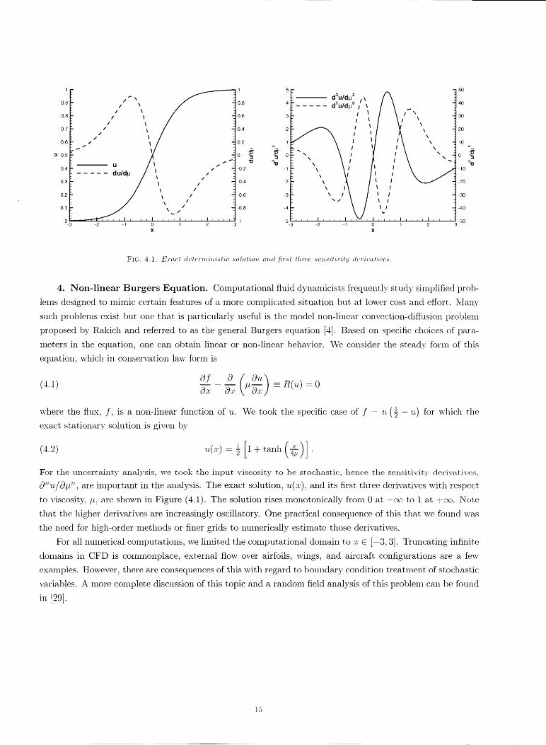
FIC. _.1. _-#_':l:o,cl (ldl, ttl"tll.'i'll.'i.h'_'L(; .ffo/'//,/,'Loll, a,',,d ./_:'r.,'t ff_,'r(:_: ._c.n..,_zl.i.c'ilfl dm".i.m,',/:t.u(:.,,',
4. Non-linear Burgers Equation. Computational fluid dynamicists frequently study simplified prob-
lems designed to mimic certain featm'es of a more complicated situation but at lower cost and effort. Many
such problems exist but one that is particularly useful is the model non-linear convection-diffusion problem
proposed by Rakich and referred to as the general Burgers equation [4]. Based on specific choices of para-
meters in the equation, one can obtain linear or non-linear behavior. We consider the steady form of this
equation, which in conservation law form is
(4.1) L?.f c9 (c9_)Oz Ox - = o
1 _ u) for which thewhere the flux, f, is a non-linear function of tt. We took the specific case of f = "u (7
exact stationary solution is given by
(4.2) "u(:c) = 7 1 + tanh V "
For the uncertainty analysis, we took the input viscosity to be stochastic, hence the sensitivity derivative.s,
O"u/Off', are important in the analysis. The exact solution, u(z), and its first three derivatives with respect
to viscosity, tL, are shown in Figure (4.1). The solution rises monotonically from 0 at -oc to 1 at +oc. Note
that the higher derivatives are increasingly oscillatory. One practical consequence of this that we found was
the need for high-order methods or finer grids to numerically estimate those derivatives.
For all numerical computations, we limited the computational domain to z c [-3, 3]. Truncating infinite
domains in CFD is commonplace, external flow over airfoils, wings, and aircraft, configurations are a few
examples. However, there are consequences of this with regard to boundary condition treatment of stochastic
variables. A more complete discussion of this topic and a random field analysis of this problem can be tbund
in [29].
15
0.9
0.8
0.7
0.6
0.5
0.4
0.3
0.2
0.1
3
IO:_
A 9 points .._,"
.... e .... 33 points _f/ 10 -_,
-_ 105
_10"
r¢
"0 10"
m010 _
A'10""
10 _:
_-_ _ I , ' = ' I ' ' ' I 10"
:---- -2 -1 .... 0 ' ' ' 1 ' ' 2 ' 3
X
, . . i _. ._,Cb.._,..._..'q.-_.-.'q,_5 10 15 20
Number of iterations
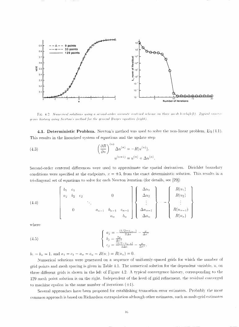
Etc. 4.2. A_um,¢.'ri,'ul .,,olMio?l.,-u,.'&W] , ._cu,'ud-o'nh"u ,ccu'r,h (cn, lc'n.d .,'+'IJcu, u on, lhrcu "m.¢._h h'vcl.,(Tcfl). 7!qp,.,I c,,rcr-
_.]_ l_(( h,'L_lov!l u,._in..q j%TEvll'lO'll',h" 'method .for /he guuc'r,,1 LY,qff'r _:q,ol'io, ('V_!lhl).
4.1. Deterministic Problem. Newton's method was used to solve the non-linear problem, Eq.(4.l).
This results in the linearized system of' equations arm the update step
(4.3) _ A_z('') - -R(u(')).
_(,,,+1) = _z(.) + A.u(,,).
Second-order centered differences were used to apl:_roximate the spatial derivatives. Dirichlet boundary
conditions were specified at the endpoints. :z: = 4-3. Dora the exact deterministic solution. This results in a
tri-diagonal set. of equations to soh;e fbr each Newton iteration (fbr details, see [29])
(4.4)
where
(4._,)
C "2
0 Ot t -- 1 _)_ _ -- 1 C,u -- 1
(1,, n b n
i ll 1
A'u,2
(l/2--ui-i) ....ZL_
O.j -- 2,",:_: -- Aa:-'
by .'XT2
(1/2-"i-- _) i:Cj -- '2/k._ _a:-' "
n('_l)
n(-..,,_ :l)
n0,.)
bl = b,, = 1, and c_1 = c_ = o,, = c,, = R(_I_) = R(u.,,) = 0.
Numerical solutions were generated on a sequence of uni:[ormly-spaced grids for which the mnnber of
grid points and mesh spacing is given in Table 4.1. The numerical solution for the dependent variable; "4L,on
three different grids is shown in the left of Figure 4.2. A typical convergence history, corresponding to the
129 mesh point solution is on the right.. Indepertdem of the level of' grid refinement, the residual converged
to machine epsilon in the same number of' iterations (4-1).
Several approaches have been proposed fbr establishing truncation error estimates. Probably the most
common approach is based on Richardsol_ extrapolation although other estimates, such as mult-grid estimates
16
10" lO -._
10 _
,,.. 10"o
10 s
.N
10 '_
._
Q 10 _
1o ._ F
til_T2
GCI estimate
Exact
FII
T I i-1 0
X
Mesh
33%
129
513
!
I r r r i I i i i 1loq ........ ;o ..... '1o•, 10 0 1 2
Mesh spacing, h
Fie;. 4.3. L+',f! - Co'n,,l;+"ql+.:'n,cc o.[ t,h.c L2 +:'rro'r "n,o'r'm, m"r.+'u,.+ 'm,c,.+h,.+'tm,ci'n, fl. l?i.qh, l - D'L+l'r_bu, tio?+ o.[ +_:/:acl a,'n,d c._'l,hn,ah,d
di.scc'rti:-:a,tio'n, c'rro'r _r_. th,'rc_.:g'rid._.
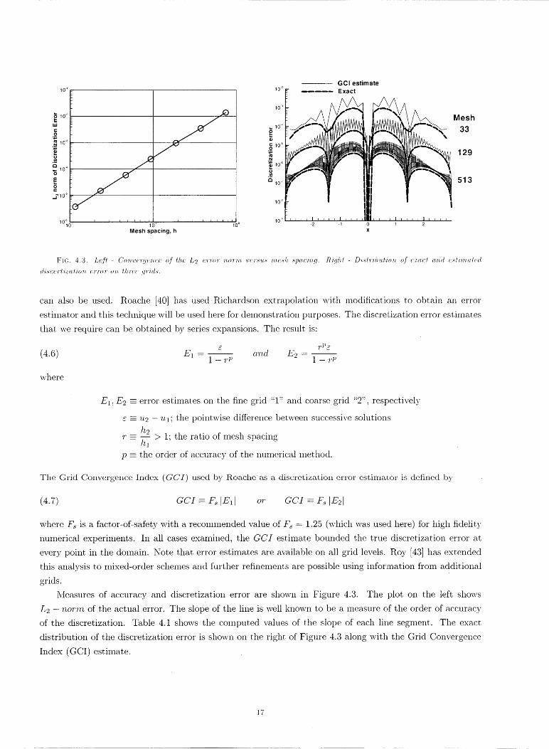
can also be used. Roache [40] has used Richardson extrapolation with modifications to obtain an error
estimator and this technique will be used here for demonstration purposes. The discretization error estiinates
that we require can be obtained by series expansions. The result is:
-- _ ar?'l,d E2 --(4.6) E1 - 1 - _'_ 1 -'r'P
where
El, E2 --=error estimates on the fine grid ':1" and coarse grid "2", respectively
c -- tL2 -_,1; the pointwise difference between successive solutions]z9
r = /-771> 1; the ratio of mesh spacing
p = the order of accuracy of the numerical method.
The Grid Convergence Index (GCI) used by R,oache as a discretization error estimat, or is defined by
(4.7) GCI _ & IE, I o_. co! _ .F_levi
where F_ is a factor-of-safety with a recommended value of F_ = 1.2,5 (which was used here) tbr high fidelity
numerical experiments. In all cases examined, the GCI estimate bounded the true discretization error at
every point in the domain. Note that error estimates are available on all grid levels. Roy [43] has extended
this analysis to mixed-order schemes and further refinements are possible using infor:mation from additional
grids.
Measures of accuracy and discretization error are shown in Figure 4.3. The plot on the left shows
L.2 - _zorm of the actual error. The slope of the line is well known to be a measure of the order of accuracy
of the discretization. Table 4.1 shows the computed values of the slope of each line segment. The exact
distribution of the discretization error is shown on the right of Figure 4.3 along with the Grid Convergence
Index (GCI) estimate.
17
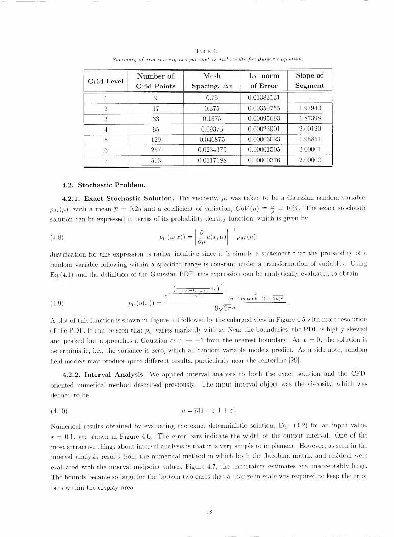
TABLE 4.1
S'wm,'m,o,'r!/ of grid co'n'ccrgc'H,c_ pwrwmcl(:r._ a,'n,d rr:._Ml,._ for Bv,'tgc'r',_" cqu_l,tio'n.
Number of Mesh L2-norm Slope ofGrid Level
Grid Points Spacing, Ax of Error Segment
1 9 0.75 0.01383131 -
2 17 0.375 0.00350755 1.97940
3 33 0.1875 0.00095693 1.87398
4 65 0.09375 0.00023901 2.00129
5 129 0.046875 0.00006023 1.98851
6 257 0.0234375 0.00001505 2.00001
7 513 0.0117188 0.00000376 2.00000
4.2. Stochastic Problem.
4.2.1. Exact Stochastic Solution. The viscosity, #. was taken to be a Gaussian randoln variable.
- _ = 10_/_. The exact stochasticP._I(#), with a mean t_ = 0.25 and a coefficient of variation. CoV(#) -- _
solution can be expressed in terms of its probability density function, which is given b_'
(4.8) p_.,(_(a:))=l_'u(:c:t_.)-' p,,: (#).
Justification for this expression is rather intuitive since it. is simply a statement that the probabilits' ofa
random variable following wittfin a specified range is constant under a transfbrmation of variables. Using
Eq.(4.1) and the definition of' the Gaussian PDF. this expression can be analytically evaluated to obtain
(., .....,,_'i., _,,,,+7) _
e 2"_ (u--l)ut.anl_ t(l--2u)'-'
(4.9) t)L'_("(:_')) = s_
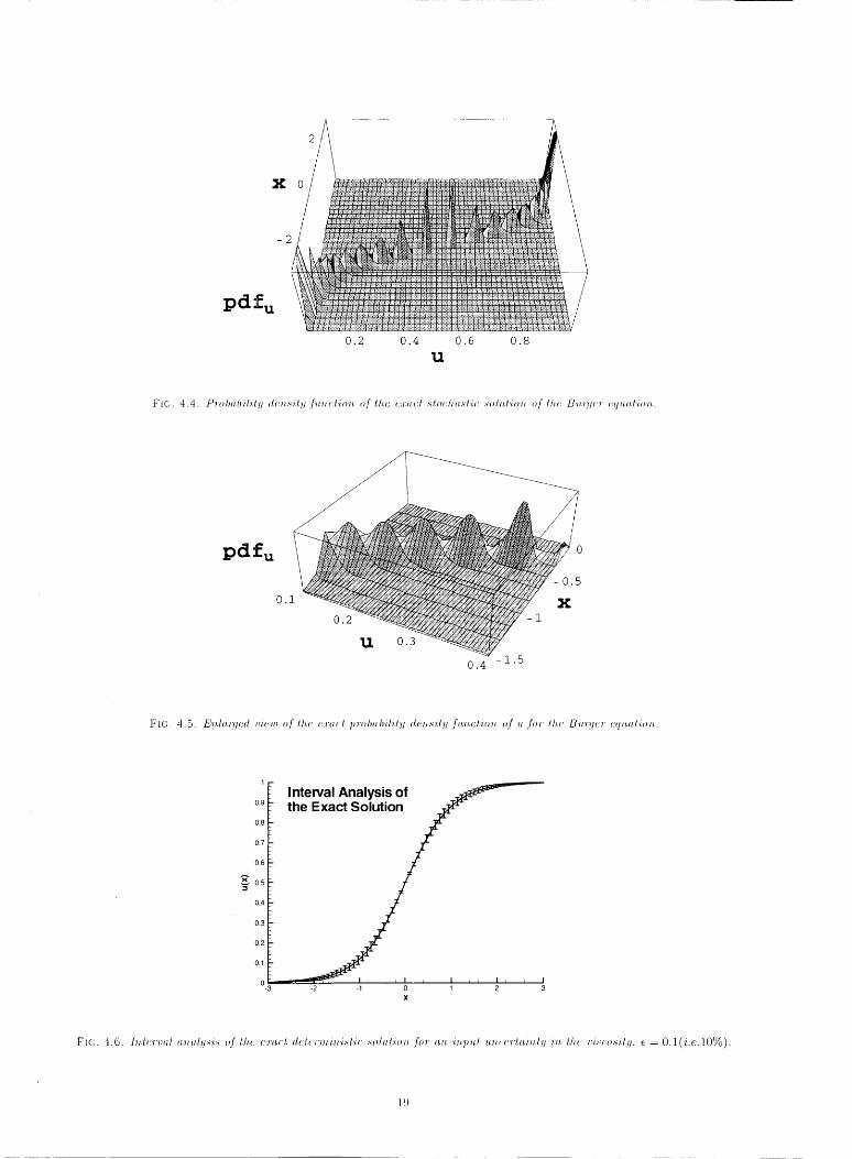
A plot of' this flmction is shown in Figure 4.4 followed by the enlarged view in Figure 4.5 with more resohltion
of' the PDF. It can be seen that Pu varies markedly with :r. Near the boundaries, the PDF is highly skewed
art([ peaked but approaches a Gaussian as :r --, 4-1 flom the nearest boundary. At .r = 0, the solution is
deterrninistic, i.e., the variance is zero, which all random variable models predict. As a side note, random
field models may produce quite different results, particularly near the centerline [29].
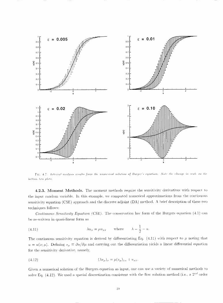
4.2.2. Interval Analysis. \¥e applied interval analysis to both the exact solution and the CFD-
oriented numerical method described previously The input interval object was the viscosity, which was
defined to be
(4.10) /_. = F[1 - c. 1 + ¢ii.
Numerical results obtained by evaluating the exact deterrninistic solution, Eq. (4.2) for an input value,
c = 0.1, are shown in Figure 4.6. The error bars indicate the width of the output interval. One of the
most attractive things about interval analysis is that it is very simple to implement. However, as seen in tile
interval analysis results from the nmnerical method in which both the Jacobian matrix and residual were
evaluated with tile interval midpoint values, Figure 4.7, the uncertainty estimates are unacceptably large.
The bounds became so large for the bottom two cases that a (-hange in scale was required to keep the error
bars within the display area.
X 0
Pdfu /
0.2 0.4 0.6 0.8
U
Pdfu o
1
0.9
o,8
o.7
0.6
0.5
0.4
0.3
0,2
0.1
0-3
Interval Analysis of ._"_"--
_ r I ' ' I I ' , I _ ' I-2 -1 0 1 2 3
Z
1 -
0.9
0.8
0.7
0.6
Ax 0.5
0.4
0.3
0.2
0.1
0 '
1
_: = 0.005 _ _ -- o._I 0.8
0,7
0.6
-_ 0.5
0.4
0.3
0.2
0.1
, I I 0-2 0 2
X
F
L_ 1_ . i i . i-2 0 2
X
1.1
1
0.9
0.8
0.7
0.6
_-i 0.5
0.4
0..3
0.2
0.1
0
-0.1
3
- _ = 0.02 _ = 0.10
2
iI . , , ; : T ' I ,
-2 2 -2 20 0
x x
F'K;. 4.T. /.nlcm:_ll _lll_l./:q.,z.._ zY,._'u.ll._ .rTO.m /lu .ll.u,,mc./-,_ua/ ._.oh#io.n o.f /3H'qH'I'._ cq_m.tion.. -'Vnh' lb.< HmnflC "Zn ._c_11_ on lhx
hollom lm_ plol.,_.
4.2.3. Moment Methods. The moment methods require the sensitivity derivatives with respect to
the input random variable. In this example_ we colnputed numerical aI)proximations from the contimlous
sensitivity equat, ion (CSE) approach and the discrete adjoint (DA) method. A brief description of these two
techniques tbllows:
Co'n, tiT_m_t.s Se't_.sitivit_q Eq'_m, tioT_ (C'5'E). The conservat.ion law form of' the Burgers equat, ion (4.1) can
1-)ere-written in quasi-linear tbrrn as
1
(4.11) Au,:,:= H_-:,::,: where ,\ = -_ - u,.
The continuous sensitivity equation is derived by differentiating Eq. (4.11) with respect to /.L noting that
,_z = "t_(:_';if). Defining s, _= _)_L/_)tl, and carrying out. the different iat.ion yields a linear different, ial equation
for the sensitivity derivat.ive, namely,
(4.12) (A.s,_,):,. = t_(,s,,)_.:,: +.t,.:<:,..
Given a numerical solution of' the Burgers equation as input, one can use a variety of' munerical methods to
solve Eq. (4.12). \\;e used a spat, ial discretization consistent with the flow solution method (i.e.. a 2 ''t order
2()
accurate centered scheme) and Newton's method. Since the problem is linear, one Newton iteration ahvays
finds the solution to machine precision (_ 10-16). It is worth mentioning that the Jacobian matrix of the
CSE equation is identical to tile Jacobian matrix of the Burgers equation. This simplifies the coding of the
CSE since one merely has to change the right hand side in the original software.
Discrete Adjoint Method. The discrete adjoint method is commonly used in aerodynamic optimization
problems ([34]) in which a user defined cost function is minimized. The cost function, denoted F('u; ;,_) where
q_ represents the i th generic design variable, is augmented with a vector of Lagrange multipliers operating
on the discrete version of the governing equations, in this case Eq. (4.1), i.e.,
(4.13) F*= F(u; _i)+ ATR(_t; g_:).
This equation is next differentiated with respect to the design variable, or more generally, any generic variable
denoted _i. After some rearrangement, one obtains
(4.14) OF* (OF ATOR.)c)u AT(0R)
Since the vector of Lagrange multipliers is arbitrary, the first term in parentheses may be equated to zero to
yield a linear system of equations for A,
(4.15) -_u a- 0u
Once the vector of Lagrange nmltipliers is known, the sensitivity of the cost function with respect to ;i can
be evaluated from
(4.16) --cgF-AT(0R)-
This basic implementation is widely used in a design environment (see [34]) and precludes the need to
compute the flow sensitivities, i.e,. c)tL/_)q4,, directly. In this problem, we require those derivatives and they
can be readily obtained by defining the set of cost functions, F = {Fj _ w IJ = 1,. 2, ...n} where ))_is the
total number of grid points. Extending Eq. (4.16) to a system of functions and insert.ing the definition of F
yields
(4.17) -_u a = -I
where I is the identity matrix and A is a matrix consisting of a set of column vectors, Aj for each j. The
required sensitivity derivatives can now be found from Eq. (4.14), which upon substitution and rearrangement
reduces to
(4.18) c9_ =AT(OR)
Note that Eq. (4.17) can be solved efficiently for all right hand sides by LU decomposition. All sensitivity
derivatives can then be computed by the single matrLx-vector multiply indicated in Eq. (4.18).
Although it may not be readily apparent, both the CSE and the DA methods yield identicM results
provided both methods are fornmlated and implemented consistently. In practice, this generally does not
occur because of differences in coding, convergence level, etc. Here, however, the equations are always solved
to machine precision, the discretizations are consistent, and consequently, the sensitivity derivatives obtained
2]
0.8
0.6
0.4
.> 0.2
_ oC"t-
_ -0.2
_" -0.4
-0,6
-0.8
-3
\
Y,,_._,__ \
[] Exact
DA
CSE
,:_llrr=_l'_=rl ..... I,,,,I
-2 -1 0 1 2 3
X
0.5
0.4
0.3
..-.i
0.2
0.1
0-3
/h
95% CI - FOSM /fy
Mean r/f
/Interval from Eq 2.3 /,_/
_- , , j
]/
j: ,
I-2 -1 0
X
FIC. 4.S. Jju.fl - Fh'.','l .',,'"H,.'_H'h"il!I fl,,:v/mllim c(*mt*u.lcfl b!/ lh_ _l/.s_'l_:l_ mrl.Frknl ,rl,Hfl ('(._rlI./'/'II.[I.()H,.'_ ._C'H,._'H/'_";I'!I m,"ll_mt.'; c_._mlmV_fl
10 lh.u ,';:l:ocl ._,_fluth,,n. R_:flhl - (..,'mn./m./rL,.,.on o.f ]ri_,_im.bil'L'.;li_, (flo..',h,r:fl /h_c.Q _'.','. H.c,n-l.,v_bo.l._il'i.'_l'ic (uv'/o/ tm_'.,;) h_l_qpr_ loli_,t_ o.f
L'll.plll H.'nccr/<vhp.t!/ _rn 2: E [--3, 0].
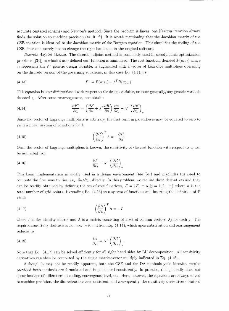
1)3; both methods are identical. A plot of the first derivative with respect to viscosity by both n|ethods is
shown on the left of Figure 4.8 and compared with the exact, derivative. The right half of the figure shows
result, s for estimating the uncertaint.y assuming that 1) the input, uncertainty (:ontains 100% of' the error
(non-probabilistic - Eq. (2.3)) and 2) a probabilistic FOSM approximation assuming that the input error
represents three standard deviations (_ 99% of the samples). The advantage of knowledge atoo_t the input
data is clearly seen in the reduced uncertainty in the output.
A comparison of the absolute error in the mean (77 = 0.2,5) and relative error in the standard deviation
(COV(/.I.) _-- _ -- 10(_,) predicted t)y Monte Carlo and the first- and second-moment n_ethods are shown
in Figure 4.9. The distribution of the mean error from the first-order moment method closely follows the
second derivative distribution shown in Figure 4.1. Adding t.he second derivative (-orrection term to obtain
the second order moment estimate of the mean results in substantially less error. As can be seen on the
right, the relative error in estimating the standard deviation is approximately 6% and 2_, tor the F()S__I and
SOS_I estimates respectively at the boundaries. One thousand MC simulations results in roughly the same
maximurn error as the SOSM method at roughly 300 times the cost. Increasing the number of simulations
an order of magnit, ude reduced the error b3; approximatel3; three at, considerable additional cost.
4.2.4. Polynomial Chaos. Sul)stituting in l)oh-nomial chaos expansions t'or the dependent variable.
t_.. and the input random variable. #. into the residual. Eq.(4.1). and t,aking the inner product. {-. @_:} yiehls
an equation for the residual of the I,/_' mode.
(4.19) R_, -- 2 Orr i=0 j=0
P P O2,u.)
-- _ _ eij_:l'i 0:,: 2i=0 j=0
where e,i.ia. - (_I_.i_.)vI_a.). \Ve iteratively solved this equation by the Euler explicit method but found that
the CPU time to achieve the machine zero steady-state solution was excessive relative to implicit methods.
Consequent.ly. Newton's method was iml)lemented by using the linearization of' the residual, which can be
'90

0.0015
0.001
oJ
_ 0.0005
,,c
d
oJ0J
-0.0005
-0.001
-0.0015-3 -2 -1
• -_ 0.01
\
.-., . i
/" " _ -0.0
"'- oo4FI- FOSM
i _ I SC)SM'o00 _10,000_. 005 MC - 1
-- _---- MC-
.... I .... I , , , r , I .... _ .... _ _0.06_31 -2 1 0 1 2 3
x
First OrderSecond Order
MC - 1,000
----_--- MC - 10,000
Fi(;. 4.9. Ab.'_olu,t<: _;'r'r_rr 'i'n, th.c 'mca'n (left) a',,d 'rcla, tivc c.'r'ro'r "mth, c ._l,(l,ll.¢t(l,'l'(] dc-cia, tio'n ('rigM,) u,._"i'n,gAJo'ntc C,'rlo ,',.d
._i'/'.h'/- (I.'11,_t N(':(;O'll, d-'lll, O'llt,(!'lLt 'llL¢:LhodN.
shown to reduce to
10(4.20) ARt,. -_ Auz = 20xi=o j=o _=o j=o
where (Szjis the Kronecker delta function. The boundary conditions were specified fl'om the exact stochastic
solution by matching moments of the distribution up to a user-specified order. The three bom_dary conditions
studied were obtained by matching
1. the mean (BC1)
2. the mean and variance (BC2)
3. the mean, variance, and skewness (BC3)
The first boundary condition, BC1, implies that the first mode, u0 is set to the mean of" the exact solution
and the remaining modes are set to zero on the 1)oundary. The second boundary condition sets u0 and ul
to the mean and variance of the exact solution, respectively, the remaining modes are set. to zero. Similarly.
BC3 sets u0 to the mean and solves a simple algebraic problem to find the values of Ul and _2 such that the
variance and skewness of the polynomial chaos distribution match the exact solution.
One advantage of Polynomial Chaos is that the output PDF's which depend on the order of the chaos
can be easily obtained. For a single random variable, the first-order chaos yields a Gaussian distribution
with mean u0 and standard deviation lUl I, i.e.,
e-(_ ....,,.,,):_/2,,i
(4.21) --
The higher-order modes account for non-Gaussian interactions and are reflected in the output PDF. For a
second-order chaos, the result is
(4.22) PPc._(u) =V/2_- lu 2 + 4u2 (u - u0 + ,_)1
Further analytic representations for higher order chaoses are possible but lengthy.
23
0.9
0.8
0.7
0.6
0.5O
0.4
0.3
0.2
0.1
0_
//_ \\ - O.02
// "1 / ;0.015
/o.ol
1// _/ i o.oo5,,.._
....... ModeO /4 .._o "_
........ Model / '_ ,,," i o.oo5
I / - -0.01
/-0.015
\ / .-,,j .... ,,-2 -1 0 1 2 3
X
0.0015
0.001
0.0005
o4
"o 0o
-0.0005
-o.ool
o.oool
5E-05
-5E-05
t /-_,
._ Mode 2 _ / \ -
...... Mode 3 t I \
_ _' '\ :
, I
', X /',;\ I\ I _ i\ l\ / I j\ j \ / _;
., , ,," / , . 3- ........-2 -1 1 2
-o.oool-o.oo15
-3 o 3
x
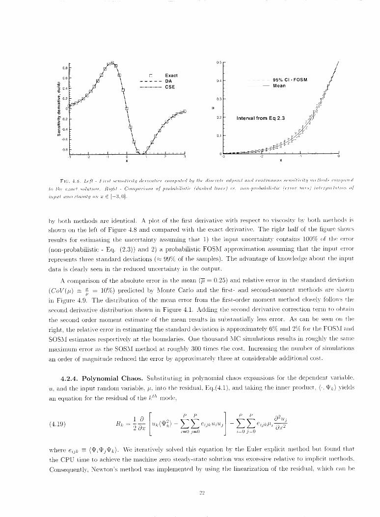
Fir..;. 4.10. Th.c .#r._'l .fou'r 'modes .flollJ Pol/lnO'mLul C'ha_._. Co'mtm.r_ to /h, ._un.._ili_'H:q dc/",;_.,_lhi_:c.,_ of lh.c _::1_1_1 .._,lul;,'u.
Numerous results were generated using Hermite polynomial chaoses of varying order with different
boundary condition treatment and on different, grids. Here we summarize these results. The first Ibm" modes
from an order 3 PC are shown in Figure 4.10. Recall that mode 0 represents the expected value (i.e., the
mean). Note the similarity of the shapes of the higher modes with the sensitivity derivatives of the exact
solution in Figure 4.1. The only discrepancy that can be seen is between the third mode and the third
derivative which is due to boundary condition treatment for this mode and will be discussed subsequently.
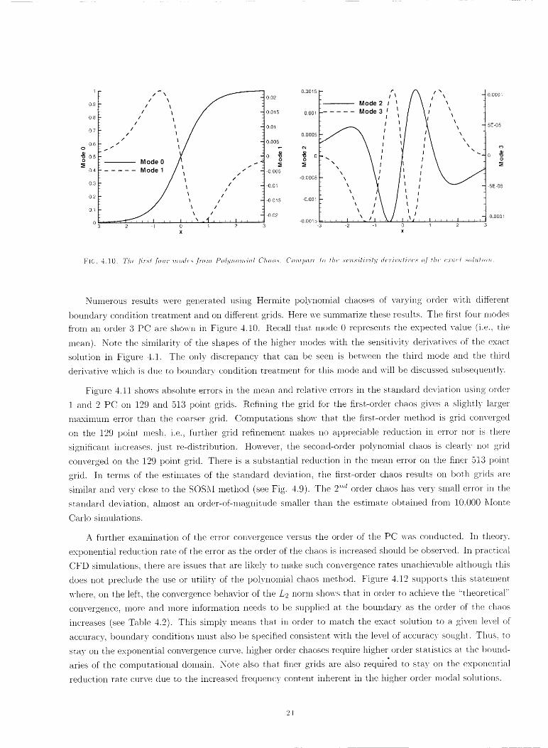
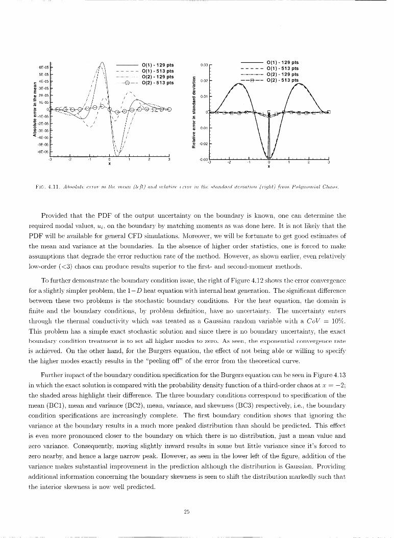
Figure 4.11 shows absolute errors in the mean and relative errors in the standard deviation using order
1 and 2 PC on 129 and 513 point grids. Refining the grid for the first-order chaos gives a slightly larger
maximum error than the coarser grid. Computations show that the first-order method is grid converged
on the 129 point mesh. i.e., fltrther grid refinement makes no appreciable reduction in error nor is there
significant increases, just re-distribution. However, the seconcl-order polynomial chaos is clearly not grid
converged on the 129 point grid. There is a substantial reduct.ion in the mean error on the finer 513 point
grid. In terms of the estimates of the standard deviation, the first-order chaos results on both grids are
similar and very close to the SOS_[ method (see Fig. 4.9). The 2 ''_zorder chaos has very small error in the
standard deviation, ahnost all order-of-magnitude smaller than the estimate obtained from 10,000 5Ionte
Carlo simulations.
A further examination of the error convergence versus the order of the PC was conducted. In theory,
exponential reduction rate of the error as the order of the chaos is increased should be observed. In practical
CFD simulations, there are issues that are likely to make such convergence rates unachieval)le although this
does not preclude the use or utility of the polynomial chaos inethod. Figure 4.12 supports this statement
where: on the left, the convergence behavior of the L2 norm shows that in order to achieve the "theoretical"
convergence, more and more information needs to be supplied at the boundary as the order of the chaos
increases (see Table 4.2). This simply means that in order to match the exact solution to a given level of
accuracy, boundary conditions must also be specified consistent with the level of accuracy sought. Thus. to
stay on the exponential convergence curve, higher order chaoses require higher order statistics at the bound-
aries of the computational domain. Note also that finer grids are also required to stay on the exponential
reduction rate curve due to the increased frequency content, inherent in the higher order modal solutions.
6E-05 _ _, 0(I)- 129 pts
5E 05 - // "\I 0(1)- 513 pts- /'/ \/ ......... O(2)-129pts
I= 4E-05 _ I / i_ ----G---- 0(2)- 513 pts
3E-05 # // / i/
E : .' I _I /--o 2E-05 - / / . il \
- / / /\'1 /.=_iE-os- / I /A _1 / / _.'_q-_.
-,E0sF ,' i', , -/ /_-2E-oag .. ,_" / /
._ -3E-05 _ ;', / .,'/'
• Ix //
.... , .... , .... , ,\?; , , .... , .... ,-3 -2 -1 0 1 2 3
X
0.03 -
0.02
o.o_
0-.=_
_, -o.o_
-0.02IZ
-0.03
0(1 ) .- 1 29 pts
0(1 ) .- 513 pts
0(2).- 129 pts
----t_---- 0(2),- 513 pts
3 -2 -1 0 1 2 3
X
]:'lC. 4.11. A l,,_ottl, tc (vr'ro'r i'n, fh,_-: 'm,c'a,'n. (lc.fl) a,'n,d rcla, f¢_:c c'r'm'r 'm. l.h,c ._'la,n, du,'rd d(:r.,ia.lio'n ('r_flh, t)..ho'm, Pol'!l_m'm,'m.l Clm.o._'.
Provided that the PDF of the output uncertainty on the boundary is known, one can determine t,he
required modal values, _, on the boundary by matching moments as was done here. It is not likely that the
PDF will be available for general CFD simulations. Moreover, we will be fortunate to get good estimates of
the mean and variance at the boundaries. In the absence of higher order statistics, one is forced to make
assumptions that degrade the error reduction rate of the method. However, as shown earlier, even relatively
low-order (<3) chaos can produce results superior to the first- and second-moment methods.
To further demonstrate the boundary condition issue, the right of Figure 4.12 shows the error convergence
for a slightly simpler problem, the 1-D heat equation with internal heat generation. The significant difference
between these two problems is the stochastic boundary conditions. For the heat equation, the domain is
finite and the boundary conditions, by problem definition, have no uncertainty. The uncertainty enters
through the thermal conductivity which was treated as a Gaussian random variable with a CoV = 10%.
This problem has a simple exact stochastic solution and since there is no boundary uncertainty, the exact
boundary condition treatment is to set all higher modes to zero. As seen, the exponential convergence rate
is achieved. On the other hand, for the Burgers equation, the effect of not being able or willing to specify
the higher modes exactly results in the "peeling off" of the error from the theoretical curve.
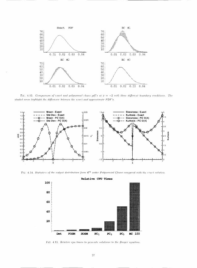
Further impact of the boundary condition specification for the Burgers equation can be seen in Figure 4.13
in which the exact solution is compared with the probability density function of a third-order chaos at z = -2;
the shaded areas highlight their difference. The three boundary conditions correspond to specification of the
mean (BC1), mean and variance (BC2), mean, variance, and skewness (Be3) respectively, i.e., the boundary
condition specifications are increasingly complete. The first boundary condition shows that ignoring the
variance at the boundary results in a much more peaked distribution than should be predicted. This effect
is even more pronounced closer to the boundary on which there is no distribution, just a mean value and
zero variance. Consequently, moving slightly inward results in some but little variance since it's forced to
zero nearby, and hence a large narrow peak. However, as seen in the lower left of the figure, addition of the
variance makes substantial improvement in the prediction although the distribution is Gaussian. Providing
additional intbrmation concerning the boundary skewness is seen to shift the distribution markedly such that
the interior skewness is now well predicted.
25

T.:, BL E 4.2
C,.._c dc.sc.liyl.W, .f,'r Figwrc 4.12
Case Condition Grid PointsBoundary
1 Mean only/ 129
2 Mean and Variance 129
3 Mean. Variance, and Skewr_ess 129
4 Mean, Variance. and Skewness 257
5 Mean, Variance. and Skewness 513
10 -s
[] Case 1
A Case 2
Case 3v
b Case 4
Case 5
, , , _ .... I2 3 4 5
Order of Polynomial Chaos
10'j
10 °;
10"1
_10 2 _-L_
1,1,1-
_ 10 -_z
E010 4
10 s
10 6
1 0 .70
N ! !! [] L. --.,
:.'\ i.\ .. -- .-.&-- - L_
- "\ 'lE ----0---- L 2
--
""
.. "_
....... "%%
I ! I ! I I I I I
2 3 4
Order of Polynomial Chaos
FK;. 4.12. E'r'ror "m. th.¢' _(J_r_" =[_¢_= _.,_'v'iou._ o'vdc'v.s o.ir Pol!l'nmwio.l (.'hao.s. Lcfl- 13wqtc'v'.s crtu_Hion milh r,_viou._ bo_llJdwr/I
co'n.dilion..s o'n.d !l'rid.s. [¢-ighl - H_-rll _qu.nlio'n with.._loctJ.o.slic i'n.lr_'ln.al hr:ol !tcnc'rolio'n..
The statistics of the distribution predicted by a 4 th order chaos are compared wit, h the exact solution
in Figure 4.14. \,Vithout symbols on the plots, the distributions are all but indistinguishal-)le. Note that the
standard deviation is a maximum in the vicinity, of :c = -1 where the PDF is nearly Gaussian as indicated
by its skewness near 0 and kurtosis value near 3. The PDF's switch from skewed to the left to skewed to
the right, in each half domain a: C [-3, 0} and :_.:_ {-3.0]. It is. also clear that the departure from Gaussian
is maximal at the boundary.
An estimate of the computational effort associated with this problem is shown in Figure 4.15. The
deterministic, first- and second-order moment methods, and polynomial chaos of orders 1-3 are compared
with the cost of 100 Monte Carlo simulations. Moment methods cost 2-3 t,imes more than a deternfirfistic
solution. The work of polynomial chaos is relatively high, about 20 times the cost, of a deterministic sohu.ion
but there are opportunities to reduce this cost (e.g. loosely-coati)led algorithms, multi-grid, ...).
2O
Exact PDF BC # 1
70 i 70 = !:!i:::!ii:!:_i.....
60 _ 60 ! _i#i[iiiii{i![!iiii::_:,
40 I 40 ::
iJ \20 ! 20 ili:;_
I0 _ i0
0.01 0.02 0.03 0.04 0.01 0.02 0.03 0.04
BC #2 BC #3
7o_ 7o:6oL 6o_
4o! 4o; / \30 30::
2oi 2oii0 _ .... l0 i
L_=_J -..... _ ,-.
\\
0.01 0.02 0.03 0.04 0.01 0o02 0.03 0.04
FIC. 4.]3. Co'tn, pa,'t'i._o'n, of c:ca, c_ a'n,d pol!l'n,o'nt.'m,l ch, a,o._' p_tf's a,L oc : -2 tr,ilh, Lh,'r_:e d'_c'rc'tl, t ho.u,'ndu:rfl co'tl, ditiotl,,_. The
,'_h,a,dcd a'r¢_,a.,'_" h.'iflh, liflh, Z l:h,c d'dJe'rc'n, cc I_cl,'mcc'n, l,h,(_ c:ra, cl _vn,d _qq_t'o:ci'm,a, te PDFb.
1.4
1.3
1.2
1.1
1
0.9
0.8
"_ 0.7
0.6
0.5
0.4
0.3
0.2
o.1{
ol
Mean- Exact - 0.03
Std Dev - Exact
.... [] .... Mean- PC 0(4)
--4--- Std Dev - PC 0(4) 0.025
'o.o ," _ ta" \ - o.o15_°
,2x
1.5
I1
0.5
o
¢./3
-0.5
-1
-1.5-3
Skewness- Exact - 5
Kurtosis - Exact
_ .... [] .... Skewness- PC 0(4) j )4.5
"_ ---'-_'--- Kurtosis- PC 014) j_ 4
3.5
3 .__2.5
2
1.5
1
1o.5
.... i .... i .... ,h, ,, _ I r r I_ I _ _ _ , o-2 -1 'o' 1 2 3
x
80
60
20
Det _ SO_ PC 1 PC 2 PC 3 MC I00
FIC. 4.].5. l_(:ht, t'i'm: cp'u, bi'm,e.s to flc'n,c'ra, t(_ ._olu.lio'n,s 1o th.e B'u,'qlC,'r _'qtt, a,t'h_,'_,.
27

/3, Shock Wave Angle _._c_
_'\'_ \ \ \ \_ \ \ " _, Deflection Angle
5. Oblique Shock Waves. Shock waves and expansion fans are fundan]ental building blocks %r in-
viscid compressible flow theory. \'Ve begin by addressing inviscid, supersonic flow over a wedge at Mach
numbers and wedge angles for which an attached, stead5-: oblique shock forms. A sketch of the problem is
shown in Figure 5.1. The output quantity of interest %r this example is the pressure rise across the shock
wave. _. which is strictly a function of the upstream _[act] nmnber. J_[] and the wectge angle 0 (for a fk\ed' PI '
/). In all cases, we take the ratio of specific heats: V = 1.4.
5.1. Deterministic Problem. For a 1)er%ct gas, the pressure rise across a normal shock wave is given
by the R.ankine-Hugoniot relation
2-,,(5.1) I)-i2= ] + _(Jl/y - 1)• t)1
where the subscripts'_:l '' and ':2" refer to conditions just ahead of and behind the shock wave respectively.
The pressure rise across an oblique shock can be obtained from the normal shock relation 1-)vreplacing
the Mach number in Eq.(5.1) by the normal component of the upstream Mach numl:)er, AIl,, in this case.
From geometric considerations,
(5.2) flI],, = AJ1 sin I3.
A relationship for the shock wave angle, !!_:can 1)e obtained from the tangential momentum equation (the
so-called d - 0 - 5i relationship). A common form of this relationship is
(5.3) tan 0 = °cot./:_ { M2sin2'3-1 }- 5I'-)(_,,,+ cos 2/3) + 2 "
For a detailed derivation, see e.g. [5]. Note that this relationship uniquely specifies the flow deflection
angle, 0, for a given Mach nmnl:)er ahead of the shock, (denoted generically by AI) and shock wave angle. 3.
However: in practice, one generally knows the _[ach numl:)er and the geometry, 0, (to within a manufacturing
tolerance), thus. one needs to solve Eq.(5.3) for .3. \\-ith some manipulation, this equation can be written
as a cubic polynomial in the variable sin 2 L_. hence three solutions f'c_)r._ exist. %r each {M, 0/ pair. Two of
the solur.ions correspond to physical processes that occur in nature: a strong shock wave and a weak shock
w_a_e although the latter is preferred by nature and is the ol_.e we study here. The third solution is non-
physical. Frequently, one uses a numerical root finding procedure such as the Secant method to iteratively
solve Eq.(5.3) for the value of ,;3 corresponding to the weak solution but here we used the analytic solution
(obtained via Mathematica v4 [46]). This was especially usefi_l fbr computing exact analytic sensitivity
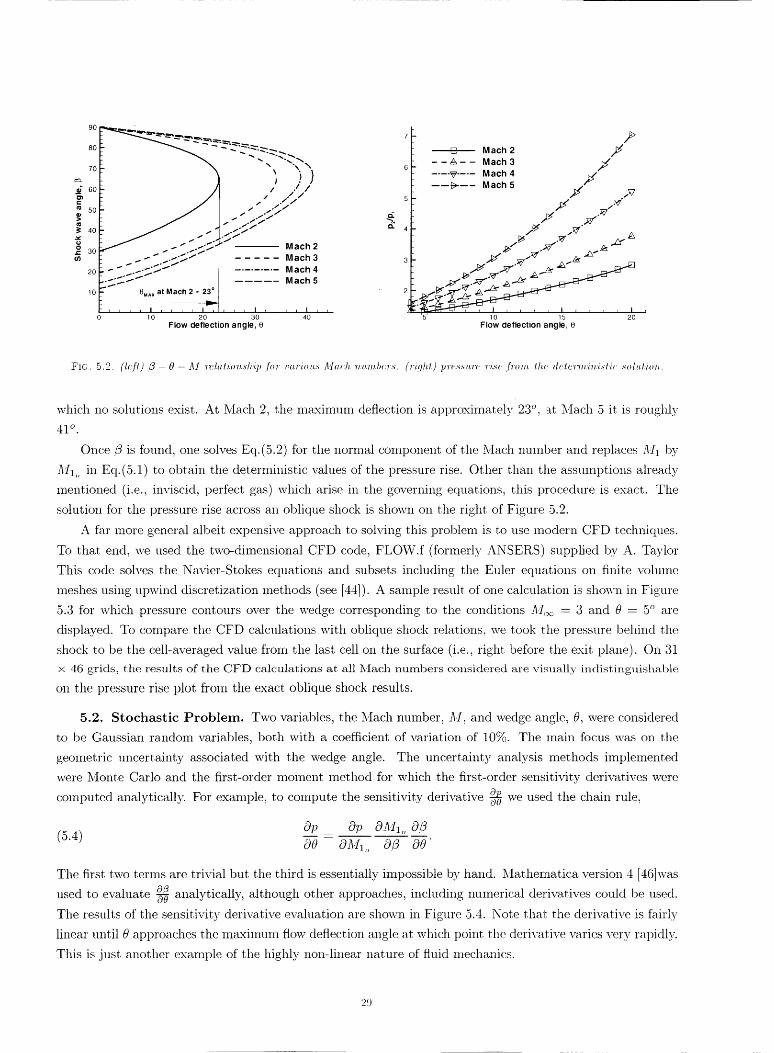
derivatives for this problem. A plot of the .,'3- 0 -/lI relationship is shown on the left. of Figure 5.2 fbr
selected Mach numbers. As can be seen. for each Mach nmnber there is a maximum deflection angle beyond
2_
d£
i(/1
9O
8O
70
60
5O
40
30
20
10
0
,, ;)j / .i /
/ / ///
_.. .t j. - /.5/
-" " ".--'_I'" ..... Mach 3
•-"" ._.-_.'_ ......... Mach 4_'_.'_'_ Mach 5
%Ax at Mach 2 = 23 °
- _ _ _ _ I I r I r I _ = = , I T _ = _ I _10 20 30 40
Flow deflection angle, 8
6
[] Mach 2--A-- Mach3
.... _,.... Mach 4----_---- Mach 5
f/
/l" .v
._'J_" H
(3. 4 J t_" _'_
3 /' ,,_ _..,,_r ._
r _-._"._--_' ._ _'-
'5' 10 15 20
Flow deflection angle, e
121(;. 5.2. (/c.[l) /_- 0- M .vela._io.,.sh.ip .[o'_ va.._'iou.._. Math. ',..,,'mbc.'_'._'. (righ.t.) p.n:._.s_,'_'e rise .fnm_. Zlu, deZe'_"m.i',.i.,'/ic ._ol,Zio',..
which no solutions exist. At Mach 2, the m_imtun deflection is approximately 23 °, .at Mach 5 it is roughly
41 ° .
Once/3 is found, one solves Eq.(5.2) for the normal component of the Mach nmnber and replaces M_ by
Ma,, in Eq.(5.1) to obtain the deterministic values of the pressure rise. Other than the assumptions already
mentioned (i.e., inviscid, perfect gas) which arise in the governing equations, this procedure is exact. The
solution for the pressure rise across an oblique shock is shown on the right of Figure 5.2.
A far more general albeit expensive approach to solving this problem is to use modern CFD techniques.
To that end, we used the two-dimensional CFD code, FLOW.f (formerly ANSERS) supplied by A. Taylor
This code solves the Navier-Stokes equations and subsets including the Euler equations on finite volume
meshes using upwind discretization methods (see [44]). A smnple result of one calculation is shown in Figure
5.3 for which pressure contours over the wedge corresponding to the conditions 2/_I<_= 3 and 0 = 5 ° are
displayed. To compare the CFD calculations with oblique shock relations, we took the pressure behind the
shock to be the cell-averaged value from the last cell on the surface (i.e., right before the exit plane). On 31
x 46 grids, the results of the CFD calculations at all Mach numbers considered are visually indistinguishable
on the pressure rise plot from the exact oblique shock results.
5.2. Stochastic Problem. Two variables, the Mach number, M, and wedge angle, 0, were considered
to be Gaussian random variables, both with a coefficient of variation of 10%. The main focus was on the
geometric uncertainty associated with the wedge angle. The uncertainty analysis methods implemented
were Monte Carlo and the first-order moment method for which the first-order sensitivity derivatives were
computed analytically. For example, to compute the sensitivity derivative _ we used the chain rule,
(5.4) 0p _ 0p 0M_,, 0/3O0 0_.I],, 0/3 O0"
The first two terms are trivial but the third is essentially impossible by hand. Mathematica version 4 [46]was
used to evaluate 0_"5g analytically, although other approaches, including numerical derivatives could be used.
The results of the sensitivity derivative evaluation are shown in Figure 5.4. Note that the derivative is fairly
linear until 0 approaches the maximum flow deflection angle at, which point, the derivative varies very rapidly.
This is just another example of the highly non-linear nature of fluid mechanics.
29
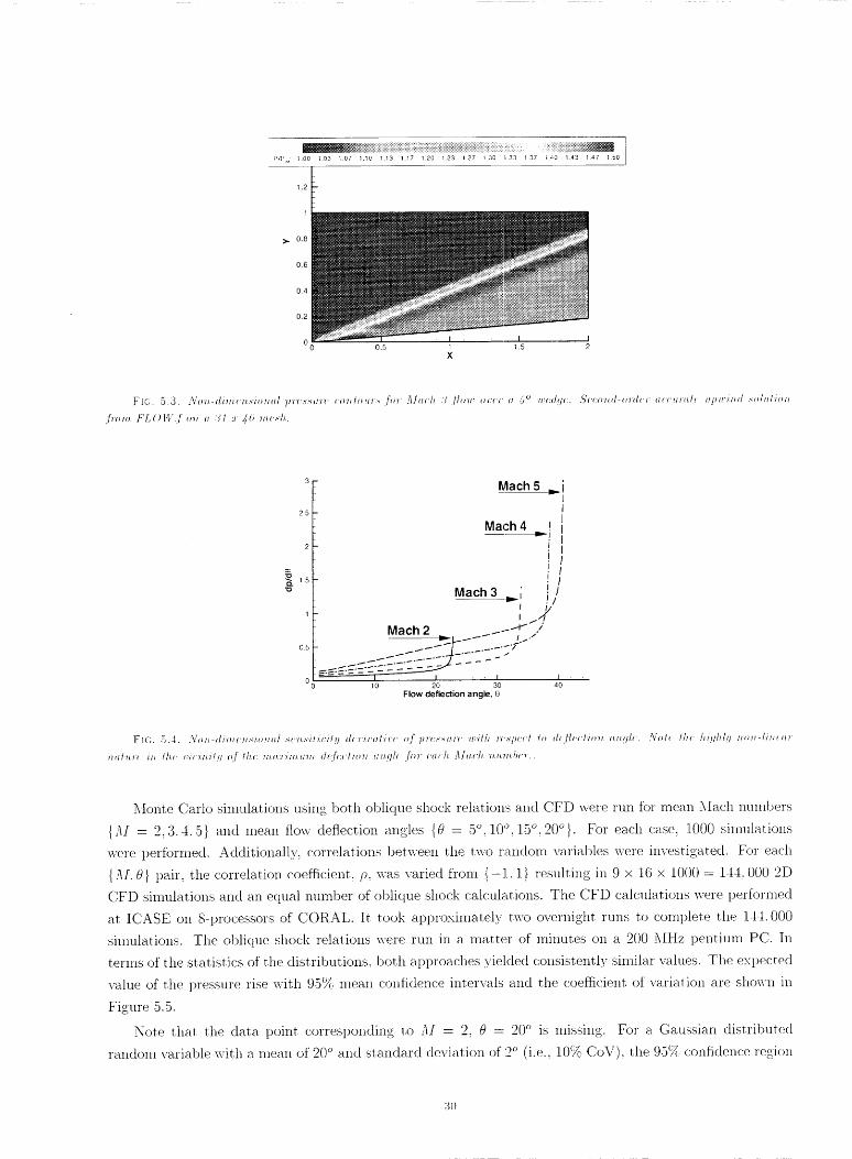
7
__iiiiiiiiiii!iiiiiiiiiii_iiiii;i_iiii_iii!i_i!i_i_i!ii_ii!ii_!i_iiiii!iii!iiii_!_i_!i_iiiii!iiiiiii_iiiiii_!iiiii_iii!!!i_ii!!i!;!i!i!i_i!iiiiiiiiiiiiiii!iiiiii!i_iii_;;:_!!i_iii!!!i!iiiiiiiii!iiiii!i!!ii!ii!iii_iPtPa: 1.00 1 03 1.07 1.10 113 1 17 1.20 123 127 1.30 133 I 37 1.40 1.43 1 47 150
1.2
1
0.8
0.6
0.4
0.2
0 I I I0.5 1 1.5 2
X
_._5
0.5
0 o
Mach 5 _i
Mach 4 !
IiI
i' !/
Mach 3 =...= ! /I I
Mach 2 --"_ /
,_.....,_ _-- _ _. _.._-7 °
--------=-"------- 22_, _"10 20 30
Flow deflection angle, O
] • ,4o
FI(-;. 5.4. _'\i_t_ dhJl._'m_io,_ll .s_"l_.._"Llil"il'!/ d_"ri_',/i_' o.f p'r,s._'u.r, u__lh 'r_'sp,_'l I, d_.flv_'lhm _llJflh. r'.\;_h' lh_. h.i_lhl!/ ,,,-/i,_,r
Monte Carlo simulations using both oblique shock relat.ions and CFD were run for mean Mach numbers
{2_] = 2.3.4.5} and mean flow deflect.ion angles {0 = 5 °. 10 °, 15 °, 20 ° }. For each case, 1000 simulations
were performed. Addit.ionally, correlations between the two r_ndom variables were invest.igated. For each
{.,'U. 0} pair, the correlation coefficient., p, was varied from {-1, 1} resulting in 9 x 16 x 1000 = 144.000 2D
CFD simulations and an equal number of oblique shock calculations. The CFD calculations were performed
at ICASE on 8-processors of CORAL. It took approxilnately two overnight runs to complete t.he 144. 000
simulations. The oblique shock relations were run in a matter of minut, es on a 200 MHz pentium PC. In
terms of the statistics of the distribut.ions, both approaches yielded consist.ently similar values. The expected
value of the pressure rise with 95% mean confidence int.ervals and the coefficient, of variation are shown in
Figure 5.5.
Note that the data point corresponding to M = 2, 0 = 20 ° is missing. For a Gaussian distributed
random variable with a mean of 20 ° and standard deviation of :2° (i.e., 10% CoV) the 95_F_ confidence region
:;(}

7
Mach 2
6 Mach 3
Mach 4
¢£ Mach 5
"6 5
==t_
> / /"
// ...Z""
/ t"/ ° _-
ILl I" _.. i ..-
I I" _'" .-- ... -"
5 10 15
Flow deflection angle, 0
,z/
//
/
//
/
/_ff' .tf t. /
f /"
t/
, , I20
0.14
0.t3
0.12
0.11
0.1
0.09
0.08
f-) 0.07
0.06
0.05
0.04
0.03
0.02
- .I-!_>
I-1 Mach 2 f/
- - ,_, - - Mach 3 _4_ _'" .-V
----_ .... Mach 4 _.." .... f _"'""
I
----!_--- Mach 5 // .,._..s- ..A" f_ ./."'" s '_'• t
_ ,7" ..-" ,,-- _ io/ f s
/ ..-
I _ z _ _ I r _ r _ I r t i _ I
5 10 15 20
Flow deflection angle, O
d'ac to ,_a'n_,pli'n, fl "ml, hu_._ of 0 .(]'l'(:',(I,_(_l' tll, o, ll, O A,la_.
TABLE 5. ]
N.,..,,,.l,r,.r of .,',.'/,,.:n/c._f,,,',,,. N/2().2) d,.,,.t ,..,.c _/.,.c,.l,cr th.a..,,0 (,,.,.t of l r)(]o).
0 ° Number of Samples > 0
Exact Values Random Draw
20 500 492
21 309 292
22 159 143
23 67 73
24 23 24
25 6 8
26 1 2
is roughly [16 °, 24°]. Clearly, when randolnly drawing 1000 samples from such a distribution, numerous
smnples will be drawn with values greater than 23 ° (see Table 5.1) which corresponds to the maximum flow
deflection angle for this Mach number hence the M = 2, 0 = 20 ° data point was rejected. To further illustrate
this, Figure 5.6 shows the input histogram with mean angle of 20 ° where numerous samples greater than 23 °
can be seen. The center and right histograms are the pressure output for input conditions M = 2. 0 = 15 °
and M = 5, 0 = 20 °, respectively for which all of the sampled angles are well below 0M,,_ for each Mach
number. In this rather academic exmnple, we chose large variations in the input variables purposely to make
the graphics easier to see, but for one case, this resulted in non-physical sampling. Such is likely to occur
with many random variables that may arise in fluid mechanics applications, for example, thermodynamic
and transport properties are bounded from below by zero whereas a Gaussian distribution has support
on [-oo, co]. One approach to overcoming this problem is to either truncate the distribution or to use
distributions with finite support (such as the Beta distribution) provided that the use of such a distribution
can be justified.
For demonstration purposes, correlations between the upstream Mach number and 0 were considered.

i00
8O
6O
4O
20
7060 8o!50 i
40 401
302O 20
i0 h ...........
16 20 24 1.8 2.2 2.6 5 7 9
025
0.2
. 0.15
%O 0.1
[] M=3, 0=5 ° j--V'"- - ,_, - - M=5, 0=5 ° f"_'"
----_---- M=5, 0=20 ° ....._...--
/._""
/"
./" _Z_
.... I I ' I I
-0,5 0 05 1
Correlation coefficient,p
The result of correlating these \:ariables is shown in Figure 5.T. As expected, when A/ and 0 are positively
co,related, the combined model uncertainty increases since increasing :l! or O independently increases the
uncert.ainty. Likewise, negative correlation reduces the variance, since one tends to off:set the other. Note that
a rather substantial variat.ion with correlation coefficient oc(:m's particularly for the stronger cases (larger
rnean 3! and mean 0). Clearly, when considering multiple random input variables, it, will be imi)o,'tant
t.o have knowledge of the (-orrelation among the variables in order to get reliable output estimates of the
variance.
:_2
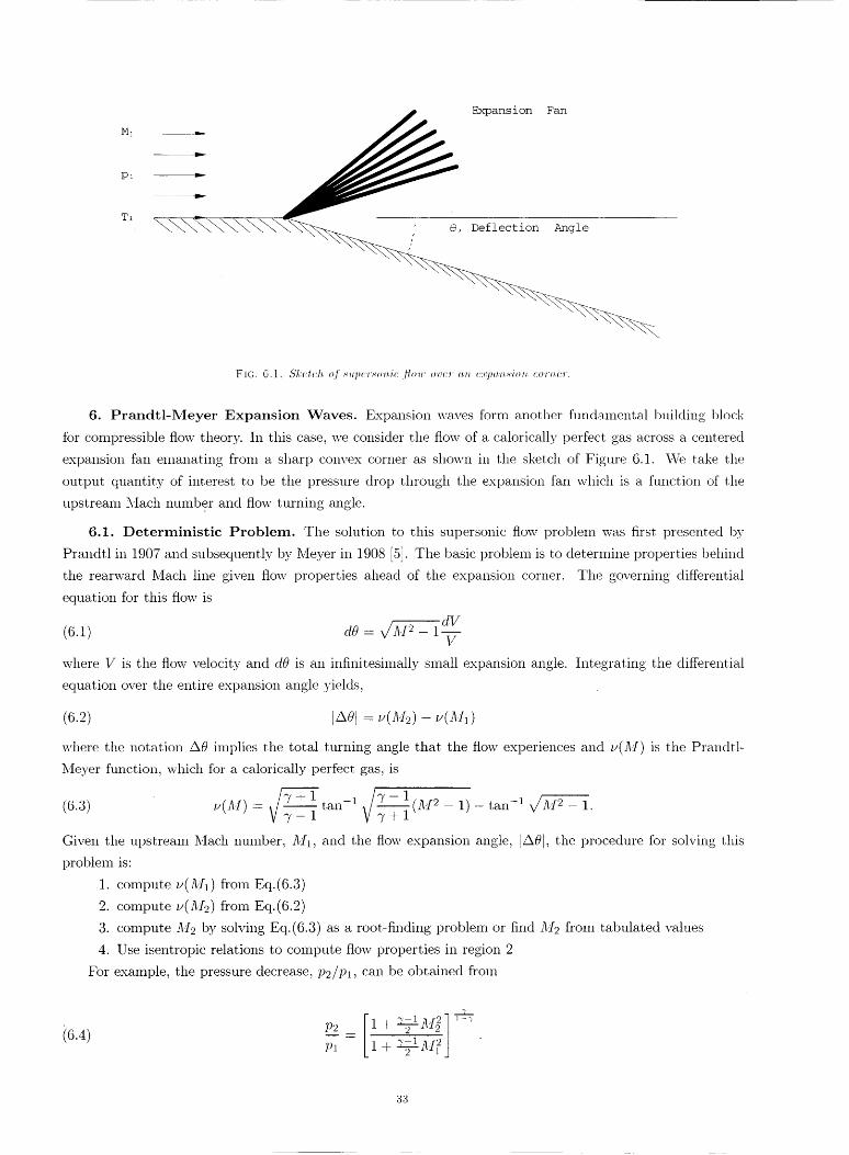
M1
Pl
T1
Expansion Fan
FIE;. G.1. ,S'L:ctch. o.f .,,'u],(_'n,_o'n.'ic ]-to'tt, o'l,cl" u.'n c:rpu.'n..','io'n, co'ln,c'r.
6. Prandtl-Meyer Expansion Waves. Expansion waves form another fundamental building block
ibr compressible flow theory. In this case, we consider the flow of a calorically perfect gas across a centered
expansion fan emanating from a sharp convex cornel" as shown in the sketch of Figure 6.1. \hze take the
output quantity of interest to be the pressure drop through the expansion fan which is a flmction of the
upstream Mach number and flow turning angle.
6.1. Deterministic Problem. The solution to this supersonic flow problem was first presented by
Prandtl in 1907 and subsequently by Meyer in 1908 [5]. The basic problem is to determine properties behind
the rearward Mach line given flow properties ahead of the expansion corner. The governing differential
equation for this flow is
dV(6.1) dO = V/M 2 - 1
where V is the flow velocity and dO is an infinitesimally small expansion angle. Integrating the differential
equation over the entire expansion angle yields,
where the notation A0 implies the total turning angle that the flow experiences and L,(]_I) is the Prandtl-
Meyer function, which for a calorically perfect gas, is
(6.3) u(]ll) = _/_+1 tan- 1 _/__] (2V/2 - 1)- tan -1 v/k12- 1.V _/-1 V7_-1
Given the upstream Mach number, All, and the flow expansion angle, [A0], the procedure for solving this
problem is:
1. compute _(M1) from Eq.(6.3)
2. compute _(z1h) from Eq.(6.2)
3. compute -/1"I2by soh,ing Eq.(6.3) as a root-finding problem or find ;I2 froln tabulated values
4. Use isentropic relations to compute flow properties in region 2
For exmnple, the pressure decrease, P2/Pl, can be obtained froxn
[_ 7--1 ,_,/-2i6.4 ) P2= + 2-''2
_..A_
53
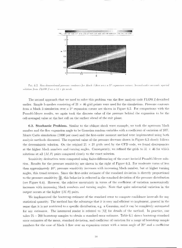
PIP,.( 0 65 0.67 0.69 0.71 0.73 0.75 077 0 79 081 0.83 0.85 0.87 0.89 0.91 093 0 95 0.97 0.99
0.5 1 t .5 2
X
The second approach that we used t.o solve this problem was the flow analysis code FLO\\;.f described
earlier. Simple h-meshes consisting of 31 x 46 grid points were used for the simulations. Pressure contours
fl'om a Mach 3 simulation over a 5 ° expansion corner are shown in Figure 6.2. For comparisons with the
Prandtl-Meyer res_flt.s, we again took the discrete value of the pressure behind the expansion to be the
cell-averaged value at the last cell on the surface ahead of the exit plane.
6.2. Stochastic Problem. Similar to the oblique shock wave example: we took the upstream Mach
number and the flow expansion angle to be Gaussian random variables with a coefficient of variation of 1()_.
Monte Carlo simulations (1000 per case) and the first-order moment method were implemented using both
analysis methods discussed. The expected value of the pressure decrease shown in Figure 6.3 closely fl_llows
the deterministic solution. On the original 21 x 31 grids used by the CFD codel we found discrepancies
at. the higher Mach numbers and turning angles. Consequently. we refined the grids to 31 x 46 for which
solutions at all {!_I, _} pairs compared closely to the exact solution.
Sensitivity derivatives were computed using filfite-difl'erencing of the exact inviscid Prandtl-Mever solu-
tion. Results for the pressure sensitivity are shown in the right of Figure 6.3. For moderate turns of less
than approximately 10 °. pressure sensitivity increases with increasing Nia.ch number, but at higher turning
angles_ this trend reverses. Since the first-order estimate of t.he standard deviation is directly proportional
a_ this behavior is reflected in the sl:andard deviation of the pressure distributionto the pressure sensitivity _,
(see Figure 6.4). However. the relative uncertainty in terms of the coefficient of variation monotonically
increases with increasing _kiach numbers and turning an_les. Note that quite substantial variation in the
output occurs at the higher {M. 0} pairs.
We implemented the bootstrap estimate of the standard error to compute confidence intervals fbr an\
statistical quantity. The nmthod has the advantage t.hat it is easy and efficient to implement: general in rlte
sense that it is not restricted to a specific distribution, e.g. a C.aussian, and it can be completel3: automated
tbr any estimator. The interested reader is referred to [12] tbr details of the method. In practice, one
takes 25 - 200 bootstrap samples to obtain a standard error estimate. Table 6.1 shows bootstrap standard
error estimates of the mean. standard deviation, and coefficient: of variation for a range of bootstral_ salnple
numbers for the case of Math 5 flow over an expansion cornel' with a mean angle of 20 ° and a coefficient
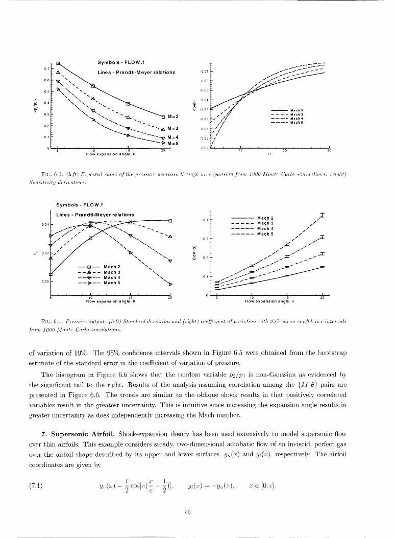
0.7
0.6
0.5
0.4
0.3
0.2
0.1
0
Symbols- FLOW.f
Lines - P randtI-Meyer relations
\_r_ "'",,. "" _ _ _ M = 2
_'_._ ""_--... " "" _'k M=3
_I_....._...2_-_..V M = 4""-!;> M=5
I _ L , , I = _ _ l I J _ _ _ I t
5 10 15 20
Flow expansion angle, 0
-0.01 L _" "" _ _"_* _--'_" _--'_""_
/I"
-o.o V ..y ---- ,.o,,.%// .... ._c._
-0.06 k/" /".//" ....... M a ¢h4
-oo_L//
oo i/-0 09
10 20 30
e
_,_ 0.0_
Symbols- FLOW.f
Lines - PrandtI-Meyer relations
._------ E]
/ / / \_._ "_,.
7" \\
,/ [] Mach 2 \x," __A__ Mach 3 \
.... _' .... Mach 4\
----I_---- Mach 5 _>
0.3
CL
>o0 0.2
0,1
= i t r I i , i r I i _ _ _ I 010 15 20
Flow expansion angle, 0
Mach 2 /_"
/Mach 3 /
......... Mach 4 //
...... Mach 5 /
// ._-'_
_/ /°/-I
//, / o
I , _ _ _ I _ _ _ _ I , _ , ; I
5 10 15 20
Flow expansion angle, 0
FIC. 6.4. P'rc,_._,.,'n, o...Lt)'.,l." (lc.f_ ) S/.a,'.,da'rd d_ucia, l i(rn. a,'n.d ('ri!lh/ ) coc._;ci(;'n.! o.r .ca,,riatio,n, .,ii.h. 96 _ "_r_],'_ (:O'n.tidc',C_' i'n.t.(_'r_..l._
f'rom 1000 Mo'n,t._'. Ca,'rlo ._i'm,'../,.,l.io'n,,_.
of variation of 10%. The 95% confidence intervals shown in Figure 6.5 were obtained from the bootstrap
estimate of the standard error in the coefficient of variation of pressure.
The histogram in Figure 6.6 shows that the random variable p.2//pl is non-Gaussian as evidenced by
the significant tail to the right. Results of the analysis assuming correlation among the {M, 0} pairs are
presented in Figure 6.6. The trends are similar to the oblique shock results in that positively correlated
variables result in the greatest uncertainty. This is intuitive since increasing the expansion angle results in
greater uncertainty as does independently increasing the Mach number.
7. Supersonic Airfoil. Shock-expansion theory has been used extensively to model supersonic flow
over thin airfoils. This exmnple considers steady, two-dimensional adiabatic flow of an inviscid, perfect gas
over the airfoil shape described by its upper and lower surfaces, y,,(z) and _(x), respectively. The airfoil
coordinates are given by
COSIer( 1(7.1) y,(x) = _ - _)], y,(x) = -y,(x). x E [0, c].
35

Number of Standard Error Standard Error Standard Error
Bootstraps in the Mean in G in CoV
100 0.000547105 0.000751298 0.0144571
200 0.000598759 0.000673770 0.0138239
300 0.000557259 0.000678446 0.0137223
400 0.000581007 0.000674247 0.0133587
500 0.000600424 O.000691841 0.0134268
0.2
0.15
>0.1O
0.05
Mach 5 Expansion Flow
Mean CoY /_ _
..... 950/°c_ _ _ _..-
_-_-_
I I , I , , I I6 7 8 9 10
Flow expansion angle, e
120 :-
: i
110 - --
100 _ i ::
80 _ . :
7O
60
, •
50 -
40 _ :
30 i M
20
lO
0 I ii0.025
..... ""-
::ii:.ii!
i_ i(i:
iiili:i_
I
0.05 0075
PiP,
0.8
M ach 50.7
0.6
0.5
0,40
0.3
02
0.1
, r'Tr_ , _1.
01 0.125 1
[] M=3, e=5 °
-- --A-- -- M=3, e=20 ° .4>".... _ .... M=5, 0=5 ° .....D_"
---- t_1_ -- -- M=5, e=20 ° .._..-t_,"
/1_. I
/
/ ._"
//z_ "" _ ._,_,..._._,._..._._._,.-.-_'
-<-'_--_'_'o'_:' ' o'''' 'o'.5.... ICorrelation coefficient, p
FIC. 6.6. L_.fl - ()..lpu, l prc._,,,'_u_- coC_n.H _l v.f I'(I,'l'HI][(kll dr." CO'l"l'('/lll',iO'll vf.f'r_<'-.,d're.m _.lh.h H,.'ml. _ ...d .,cdfff .n_l h . O.
];',qlh, l - Hi.,,loflr..'m, vf th.c vMpu.l p'rcs.,.'u.'r_ di._trZh.lhm. .t ,'II.H_ 5 th,'r_qlh _. c.rtm'H,.,_ion .,ith. . "m.c.'n. .WII_ o.f 20 ° ..d . IH_;"
cm:./_fr'ir"nl of mrrmlhm.. :¥vlu th_l lhu di..drH_ul_<m i..._ .,J<cu:u/ lv the 'r41hl.
:36
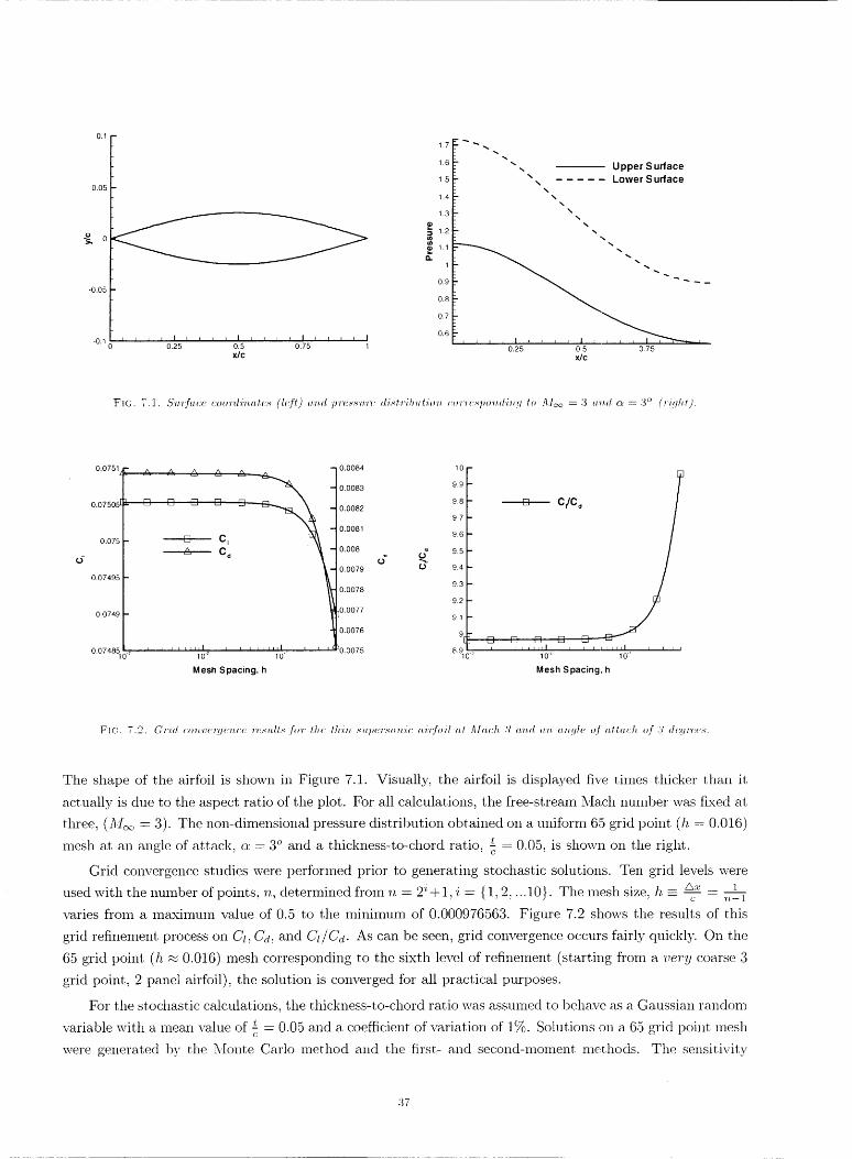
0.1 -
0.05
o_, 0
-0.05
-0.10
i i _ i I I r i i I _ r I I I K r i I I0.25 0.5 0.75 1
X/C
1.7
1.6
1.5
1.4
1.3
_ 1.2
_ 1.1
1
0.9
0.8
0.7
0.6
" ,, Upper Surface
" Lower S urface
%%.
.%%
.%
0.25 O.5 0.75_C
FK;. 7.1. Stt'/fa.cc coo'rdi'n.atc._ (left) a.'n.d p're.,'.s'u.'rc di._t'rit)u.tio'n _:o'rrc.,'po'n.di_Jg to .h/_ : 3 a.'n,d c_ = 3 ° (rtqh.t).
0.0751
0.0750_
0.075 -
0.07495 -
0.0749 -
J. []
A A & A _,..._,&
[] [] [] []
[] C_
A C d
0.07485 0 102 10 _
Mesh Spacing, h
- 0.0084
0.0083
0.0082
0.0081
0.008
o.o079
0.0078
0.0077
0.0076
r rz 0.0075
10-
9.9-
9.8-
9.7-
9.6-
9.5-
9.4-
9.3-
9.2-
9.1 -
9[_-8.%b_
[]
[] [] []i i r i lilT[
10 _
c/c,
I I I I I IIII I r I I10":
Mesh Spacing, h
FIe_;. 7.2. C_'i(l co'n, ve_fle_J,('c ,rc.,'u, lt._ fo'r the th, in.._'upc'v._'o',.i(: ,.i'rfoil ,/ ]ll,,(:h, 2 a,'n.d o.'n. o,'n.gle o.f' ,,tt,,(:h, of 2 duprcu._'.
The shape of the airfoil is shown in Figure 7.1. Visually, the airfoil is displayed five times thicker than it
actually is due to the aspect ratio of the plot. For all calculations, the free-stream Mach number was fL'ced at
three, (2/.I_ = 3). The non-dimensional pressure distribution obtained on a uniform 65 grid point (h. = 0.016)t
mesh at an angle of attack, ct = 3 ° and a thickness-to-chord ratio, g = 0.05, is shown on the right.
Grid convergence studies were performed prior to generating stochastic solutions. Ten grid levels were
used with the number of points. _z. determined from n = 9i+ 1. i = {1, 2, ..10} The mesh size. h = _'_ -• , " ' , " " ' c 'n.--1
varies from a maximum value of 0.5 to the minimum of 0.000976563. Figure 7.2 shows the results of this
grid refinement process on Cz, Ca,, and CI/C_,. As can be seen, grid convergence occm's fairly quickly. On the
65 grid point (h _ 0.016) mesh corresponding to the sixth level of refinement (starting from a ver_j coarse 3
grid point, 2 panel airfoil), the solution is converged for all practical purposes.
For the stochastic calculations, the thickness-to-chord ratio was assumed to behave as a Gaussian random
variable with a mean value of _ = 0.05 and a coefficient of variation of 1%. Solutions on a 65 grid point mesh(:
were generated 1)3' the Monte Carlo method and the frst.- and second-moment me, thods. The sensitivity
37
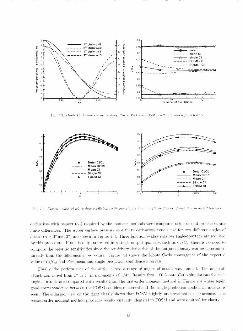
98_"_ 1 ,t deriv e.=O
._ 7 F_: _, _ 2"_ deriv c_=0
6 _- \ (".. _ ......... 1" deriv c_.=3
5I \\\ "'"'"X ..... 2 _ deriv o:=3 //
E 3 \'_\ "'X'_X " i i
.7: ,, ,,;,"o x tt, 'XI /5 /
• -' \t, "N. ,9"-2 \\ _-.. / /
\ .,; _ ......-5 I ' r ] , ,, ,, "'_..J._ , _ I ,
0.25 0.5 075X/C
9.2
40•= 9.15_
35 "E9.1
O30 "_
9.05
25 03, {j_ 9/"
20 _ 0• 8.95._
15 mm 8.9o9
lO _ 8.85-
(n5 .o 8._
__ _ _ .... ---Otto[] mean
mean Cl
0 single CI
FOSM - CI
. "-.. _ _ - ........ SOSM - CI
- - D ..... qt. ----D-_---C]
i ; , ..... I ....... I10_ 10
Number of Simulations
FIe;. 7.3..4hm.h _.'(I'FI() ('o'uccqlc',.<:<" DL_h_r!l. The FO,S'3I u.',,d S()S.4/ 'r('.+,/l._" a'r< ._Im,", ./'o'r r(:.fcrc,(<.
9
8.5
8
7.5
db" 7
6.5
6
5.5
I]-A7 _ Mean Cl/Cd
/// ......... Mean Cl
_r/ -- .- Single Cl
Z =- FOSM CI
, , , , I .... I t r , I I .... I2 3 4 5
9.2
9
A
8.9
_8.8(..)
8.71
8.6
8.5i
// t" f
2/" t"
_.. /._._/t -''°
• Deter Cl/Cd.//>" _ Mean CI/Cd
/_/ Mean CISingle CI
FOSM CI
8._- = _ ' ' I , , , L I , , , = I .... I_25' 2.75 3 3.25 3.5
(7.
Fic. 7.4. E.rt,<:t<d _;a.lux o.f lifl-to-dr_ql r'ou.tfi<:ic'nl._ u,_lh. u.'n.c<'rhrh_l!/ d_u' to <_ J/',/ c(,,._:ciu'nl qf t,armlLo'n, i'll _I'LI:/'I,'I/ thbl.n(._.,'.
derivatives with respect to L required by the moment methods were con-iput.ed using second-order accuratec "
finite differences. The upper surface pressure sensitivity deri,,;atives versus :c/c for two different angles of
att, ack (o. = 0 ° and 3 °) are shown in Figure 7.3. Three function evaluations per angle-of attack are required
1)y this procedure. It' one is only int, erested in a single output quantity, sucli as C'_/C.'<z, there is no need to
comput.e the pressure sensit, ivities since the sensit.ivit.x, derivative of the out.put quantity can l:)e der.ermined
directly from t.he differencing procedure. Figure 7.3 shows the Monte Carlo convergence of the expected
vahie of C_/C<_ and 95% mean and single prediction confidence, intervals.
Finally, the performance of the airfoil across a range of angles of attack was studied. The angle-of-
attack was varied from 1° to .5° in increments of 1/4 °. Results fl'om 100 Monte Carlo simulations for each
angle-of-at.tack are compared with results fl'om the first-order moment method in Figure 7.4 where a_:ain
good correspondence between the FOSM confidence interval and t.he single prediction confidence interval is
seen. The enlarged view on the right clearly shows that FOSM slightly underestimates the variance. The
second-order moment method produces results virtually identical to FOSM and were omitted for clarity.

8. Laminar BoundaryLayer Flow. Theboundarylayerequationsfor steady,two-dimensionalin-compressibleflowwithconstantpropertiescanbewrittenas
(8.1) 0u 0v+N =0
Ou O_L U dU 02u(8.2) + =0y
subject to the boundary conditions
(8.3)
It is well known that these partial differential equations can be re-cast in terms of a sinfilarity variable as an
ordinary differential equation for which solutions exist for specific freestrealn velocity distributions, U(x).
In 1908, Blasius found a solution to the parallel flow over a flat plate with U(x) a constant (see [45]). Under
these conditions, the governing equations in self-sinfilar form reduce to
(8.4) f'" + f f" = 0
where f = f(_?) only and
(8.5) u(x,y) = U(:c)f'O] )
The boundary conditions transibrm to
where v/U_](z, y) = y 2ua'"
(8.6) f(O) = if(O) = 0 ,f'(oo) = 1
To date, an analytic solution to this equation is not known although series solutions with a finite radius
of convergence are established. Numerically, the problem reduces to finding the value of f"(0) such that
f' _ 1 as 'q _ oc. An asymptotic analysis shows that _7= 10 is a sufficiently large value. Finding the correct
value of f'(O) is a simple root finding problem which, in our calculations, was solved by the Secant method.
The correct value to six significant digits is (see [45])
(8.7) f"(0) = 0.469600. • •
8.1. Deterministic Problem. A relatively fine 5000 grid point mesh distributed on 77C [0, 10] was
used for the numerical solution. Similarity functions and velocity profiles x = 1 meter for three different
freestream Reynolds numbers (Re - u,_) are shown in Figure 8.1.M J
8.2. Stochastic Problem. The kinematic viscosity, u, was taken as a normally distributed stochastic
input parameter with a coefficient of variation of 2%. The sensitivity derivative required for the FOSM
method can be obtained from
(8.8) au _ ou o,? _ u)? f,,(,l).Or' 0_10u 21/
The second derivative (for the SOSM method) can be found by further application of the chain rule to be
(8.9) Og-u _ U,1 (3f'('q)+ 'l.f'"('l))Ou 2 4u 2
39

1.5
._o
2 1
r_
0.5
0 0
f(q) /
f'(q)
......... ,,
1 2 3 4
q
/iol -_ ....... _" _ _
0.9
0.8 _- ii// ///i
o7- /' / ,'
0.6 //1111Re = 5,000o.5
i1/ / Re= 10,000
0.4 // // ......... Re=20,000
_//i /0.3 i /0.2
,1'//I
00, _ ' ' ' I _ _ r _ I .... I .... I0.025 0.05 0.075 0. t
y (meters)
0.4
0.3
0.2
._>
0.1
'_ -0.1
g-0.2
-0.3
-0.4
I/ /" I ...\ duldv
/// '_X\ d2u/dv 2
I \I \
r _ I I t I I T I2 4 6
q
0.0008
0.0007
.__0.0006
13 0.0005
"_ 0.0004
0.0003
0.0002
0.0001
0i
/ \ MC- 1o00@ --Q-- FOSM
.... [] .... SOSM
05 ::::::_:::bd_y/8
YI(;. 8.2. ,Vo,-d.ml.c.,.._.,m.n.ol ._c.,..,../l.i,;./t:q dc'rh_ot/rc._ (/c.fl) ,',.d dL_l.ribu.l.m._ of lh.c t_r:.lm./l.!l ._l,'nd,'nt dcr'mlio, th'm,flh lh_
bo u.H,d_ vii l,/l_"v.
Plots of _l_e derivat.ives, non-dimensionalized by U and t.he mean viscosit.y. 7v. are shown in Figure 8.2.
For this problem: t.he contribut.ion of the second derivat, ive terms t,o the estimat, es of t,he mean and variance
are negligibly small and hence their distribut, ions are indist, inguishable as seen on the right, of Figure 8.2
where t,he Mont, e Carlo result, s after 1000 simulations are also shown for comparison.
Mean velocity profiles at, a: = 1 meter and Re = 10. 000 ol)t, ained fi'om 1000 Monte Carlo realizations
are shown in Figure 8.3. An enlarged view is display,:ed on t,he right so that the single predict, ion confidence
int, ervals can be readily observed. The FOSM and SOSM confidence intervals coincide wit, h the _Xionte
Carlo confidence int, ervals and were omirted in the plot for clarify. It is worth noting that, the 95% mean
confidence int, ervals are smaller by a factor of' roughly 30 (_ V 1_0--0-0) and should be used for giviitg the l_est
estimate of the mean. However. since n_oment-based met.hod,_: only estimat, e the standard deviat, ion of the
parent, l:_opulation, a more direct comparison t,o Monte Carlo i:s afforded 1:6; the single prediction confidence
intervals.
1()

0.75
0.5
0.25
Mean95% CI
0.25 0,5 0.75 1
y/5
Mean
95% CI ,.. _ =
/ I i t
/ / / t
/ ff /
f J
07S0ra .... I• 0.75
y/6
G)
¢..t"o
-8¢..
o
0.001
0.0008
0.0006
MC
i FOSM
• , I _ I I I
250 500 750 1000
Number of Simulations
FIC;. 8.4. Coilvc.'rfl_m,c_: of Bqml, te Carlo sim'_l, lo.lio'n,_ _l,l,y =0.17 'm,cl,(-:'l'.s.
The convergence of the standard deviation predicted by the Monte Carlo method versus the number
of simulations is shown in Figure 8.4. The FOSM and SOSM estimates (which lay on top of one another)
are also shown. Note the relatively slow convergence of the Monte Carlo method as can be seen by the
low frequency meandering of the velocity standard deviation. If one wants very accurate estimates of the
standard deviation, this slow convergence and hence high cost will be unacceptable. However, if one only
needs a moderately accurate estimate of the mean and is willing to accept a fairly rough estimate of the
standard deviation, then relatively few simulations may yield acceptable results.
9. Summary. This paper reviews deterministic and probabilistic uncertainty analysis methods applied
to fundamental problems in fluid mechanics. Sources of uncertainty and a discussion of selected methods
for random variable models are presented. Applications presented include a linear convection problem with
a source term, a non-linear Burgers equation, supersonic flow over wedges, expansion corners, and a thin

supersonicairfoilaswellasincompressibleboundarylayerflow.Themethodsdiscussedandimplementedare:IntervalAnalysis,Propagationof errorusingsensitivity
derivatives,MonteCarlosimulation,MomentmethodsandPolynonfialChaos.Althougheasyto imple-ment,intervalanalysisoftenresultsin maximalerrorboundsthat arequitelarge.ThebasicprocedureforimplementingMonteCarlois presentednext. Althoughcomputationallyintensive,MonteCarlosolutionsarefrequentlyusedasa baselinefor comparisonwithothermethodssincetheyareknownto convergetotheexactstochasticsolutionin thelimit of infinitesamplesize.First-andsecond-ordermomentmethods.popularbecauseof therelativelylowcostandutility in a designem:ironmentarecovered.ThesemethodsgenerallyyieldgoodapproximationswhentheoutputprobabilitydensityfunctionisaGaussiandistributionor relativelycloseto Gaussian.Next.Hermitepolynonfialchaosisdescribedforsolvingstochasticproblemsinvolvingrandomvariables.Themostsophisticatedofthemethodsreviewed,polynomialchaosisbasedonaspectralrepresentationoftheuncertaintywhichissubsequentlydecomposedintodeterministicandrandomcomponents.Often,highlyaccurateresultsareobtainablefromthisapproachat lowercostthanXionteCarlosimulations.
All methodswereimplementedfora non-linearformof thegeneralizedBurgersequationforwhichweobtainedanexactstochasticsolution.Tomimicthebehaviorof CFDcodes,weusedsecondorderspatialdifferencingandix-nplement,edNewton'smethodto soh,ethenon-linearproblem.In allcases,approximatelyteniterationswererequiredto achievemachineprecisionresults.Intervalanalysiserrorboundswereunac-ceptablylarge,evenwhenperformedasasinglefunctionevaluationout,sidetheiterationloop.Bothfirst-andsecond-ordermomentmethodsproducedreasonableestimatesofthemeanandvariancebut thesecondorderestimatesweresubstantiallybetter.Polynomialchaossolutionsofvariousordersweregenerated.Thefirst-orderchaossolutionswerecomparableto thesecondmomentsolutions.Thethird andfourth-ordersolutionswereveryaccurateandmatchedtheexactPDFof thesolutioncloselyat all point,sin thedomain.\\:ealsoshowedthatthetreatmentofboundaryconditionsandthequalityof thegridhasanimpactonthe
error convergence as a function of the order of the chaos.
Oblique shocks and expansions were considered in which the flow turning angle and the input _iach
number were considered to be random variables. We used the 2 - D CFD (:ode FLOW.f as well as shock
expansion theory to simulate these flows by the Monte Carlo and first-order moment methods. Parametric
results showing the impact of correlation among the variables demonstrate the need to have knowledge about.
the relationship among input random variables. Supersonic flow over a thin cosine shaped airfoil was studied
at a variety of angles-of-attack. The thickness of the airfoil is treated as a random variable and the impact
of this uncertainty on the lift-to-drag curve is examined.
Finally, we studied incompressible, steady flow over a flat plate, the celebrated Blasius flow. in which the
kinematic viscosity was uncertain. The equations were solved in self-similar variables for which the random
variable gets folded into the similarity variable. Both moment methods and Monte Carlo simulations were
performed. For this example, little difference was observed between the first- and second-moment methods.
REFERENCES
[1] D. P. AESCHLIMA.X AND \\7. L. OBERI,2AMPF. Ezpe'li?n, entcd meth, odolo9_ .[b'l com])_._,tatiortal .fl'_Lid @-
'lzo,rnics code v(flid_Ltio'n, AIAA Journal, 36 (1998), pp. 733 741.
[2] AIAA APPLIED AERODY_XAMICS TECI-J_',ICAL CO._INIITTEIZ: D?"c_9 P_'edictio'n, Wo'r'_:sho'p, 19 _h APA Co'_z-
.[ere_zce, Anaheim, CA. 2001. http://www.aiaa.org/tc/apa/dragpredworkshop/dpw.hunl.
49_

[3] Guide for the verification and validation o.f computational .fluid dynamics simulations. AIAA Guide
G-077-1998, 1998.
[4] D. A. ANDERSON, J. C. TAXXEHILL, A.X-D R. H. PLETCHER, Computational Fluid Mechanics and
Heat Transfer, Series in computational methods in mechanics and thermal sciences, McGraw-Hill,
1997.
[5] J. D. AXDE1_SO.X, Modern Compressible Flow, McGraw-Hill, New York. USA, 1982.
[6] T. J. BARBER, Role of code validation and certification in the design envi'mnment, AIAA Journal. 36
(11998), pp. 752-758.
[7] J. A. BENEI,:, E. 5,i. IS:RAFT, AND R. F. LAUER, Validation issues for engi_te-ai_frame integration,
AIAA Journal, 36 (1998), pp. 759-764.
[8] C. H. BISCHOF, G. F. CORLISS, L. L. GREEN, A. GPdE\V:,_.\b:, K. HAICLEa, AND P. A. NE\VMAX,
Automatic d'_ifJ'erentiation of advanced CFD codes Jbr multidisciplina'ry design., Jom'nal on Computing
Systems in Engineering, 3 (1993), pp. 625-637.
[9] G. DAHLQUIST A.XD A. BJORCK, Numerical Methods, Series in computational methods in mechanics
and thermal sciences, Prentice-Hall, 1974.
S. DOLLIN-G, High-speed turbulent sepa'r'ated .flows: Consistency o.f mathematical models and .flow
physics, AIAA Jom'nal, 36 (1998), pp. 725-732.
E. TURGEON- AND J. BORGGAARD, Sensitivity and uncertainty analysis .for variable property .flows,
AIAA-paper 2001-01_0, in 39 th AIAA Aerospace Sciences Meeting and Exhibit, t:{,eno, NV, January,
2001. CD-ROM.
EFRON AXD R. J. TIBSHIRANI, An Introduction to the Bootstrap, Chapman and Hall, New York,
NY, USA, 1993.
E. GARZON AND D. L. DARMOFAL, Using computational fluid dynamics in p'rvbabilistic engineering
design, AIAA paper 2001-2526, in 15th AIAA Computational Fluid Dynamics Conference, June
11-14, 2001.
GHANEhl, Stochastic .finite elements with multiple random non-gaussian properties, Journal of Engi-
neering Mechanics, (1999), pp. 26-40.
GHANEM AND P. D. SPANOS, Polynomial chaos in stochastic .finite elements, Journal of Applied
Mechanics, 57 (1990), pp. 197-202.
G. GHAXEM, Ingredients for a general purpose stochastic .finite element formulation, Computational
Methods in Applied Mechanical Engineering, 168 (1999), pp. 19-34.
G. GHAXEM AND P. D. SPANOS, Stochastic Finite Elements: A Spectral Approach, Springer-Verlag,
New York, 1991.
G. GODFREY, Topics on Spatially High-Order' Accurate Methods and Preconditioning for the Navier-
Stokes Equations with Finite-Rate Chemistry, PhD thesis, Virginia Tech, 1992.
G. GODFREY AND E. _f. CLIFF, Sensitivity equations .lbr turbulent flows, AIAA-paper 2001-1060,
in 39 th AIAA Aerospace Sciences Meeting and Exhibit, Reno, NV, January, 2001. CD-ROM.
L. GREEX, P. A. NEWMAN, AXD K. HAIGLERI Sensitivity derivatives for advanced CFD algorithm
and viscous modeling parameters via automatic differentiation, Journal of Computational Physics,
125 (1996), pp. 313-324.
G. HABASHI, J. DO.klPIERRE, Y. BOURCAULT, _'I. FORTIN, AND _[. WALLET, Certifiable compu-
tational .fluid dynamics through mesh optimization, AIAA Journal, 36 (1998), pp. 703-711.
HALDAR AND S. 5IAHADEVAN, P'mbability, Reliability and Statistical Methods, in Engineering Design,
[111D.
[12] B.
[13] V.
[14] R.
[15] R
[16] R.
[18] A.
[19] A.
[20] L.
[21] W.
[22] A.
43

John Wiley and Sons, Inc., 2000.
[23] A. HALL, 07_ a_ ezpe';'irn, e_tal det_er'mi_atio_ o.[ To, Messeng. Math., 2 (1873), pp. 113-114.
[24] J. M. HA.,Xl.klEI_SLEY AND D. C. HAXDSCOMB, Mo_,te Ca,_lo Methods. Met.huen's Monographs on Ap-
plied Probability and St,at,istics, Fletcher & Son Ltd., Norwich. 1964.
[25] J. C. HELTO.X .aND F. J. Davis, Sampling-based methods fo'r '_,_ce'rtai'_t_t a_zd seT_sitivit_] aT_,algsis: Tech.
Report SAND99-2240, Sandia Nat,ional Laboratories, July 2000.
[26] L. Hu'csI-=, F_'ee-.fbTrn ai_:lbil shape optimization tLr_de_" _L_zce_'taint_ _tsiTzg _Tza:cirr_:_L'nzezpected z_al'_te
a'_zd seco_zd-oT_de_" seeo_d-mome_z_ st,r'ate9ies, t,ech, report., ICASE Report 2001-18/NASA CR 2001-
211020, 2001.
[27] --. Solvi'lzy PTvblems o.f O'l)_,i_Tzizatio_z U'_u].e_"UTzce'rl,o,i'_zt:qa._ St, at,isl,ical Decisio'_z P'_vblerr_s. AIAA-
Paper' 2001-1519, in 42 '''_ AIAA/ASME/ASCE/AHS/ASC \tract,ares, St,ructural Dynamics. and
Mat.erials Conference and Exhibit, Seattle, \'_L_, 2001.
[28] L. HLYSE AXD R,. M. LE\\_S, Ae'ro@'_za_de shape ol)tir_,izatio_z o.f t_vo-dime_sio_zal aiA'oil._ '_,de'_ '_,,-
cer't,a i_ co_zdit, io'rzs, t,ech, report, ICASE Report. 2001-1/NASA CR 2001-210648, 2001.
[291 L. HUYSE A.XD R. \\,:. \'_'ALTElZS, _a_zdoTn, field sol_tio';_s i';_cl_tdin 9 bo_';_,da_'9 co';zditio';z ._;,ce'rtai';zt#
./'o7' the stea@-state gerze_'alized bu,_:ge_' eqv,atio'_z, tech. report, ICASE Report 2001-35/NASA CR
2001-211239, 2001.
[30] A. JA_[_SOX a.xI? L. _[ARTI.XELLI, Mesh _'(__i'_zeme'nt a'n,d modeli'n,.y e'r'ro'rs i_z .flo'_v simv, latio_zs: AIAA
Journal, 35 (1998), pp. 676--686.
]31] L. K_Lk:IN, Ni'_zetee_zth ce'_zt_'y clo'ads ove_" the @_za,rnical theo_-'9 of hea_ a_d light, Phil. Mag., 2 (1901),
pp. 1 40.
[32] M. D. McKa'c, R..J. BECb:,.xIaX, a.XD \,V. J. Coxox'EP_, A compa'riso'n, o.f th_'ee methods o./' selecf, i'_z9
val'aes o./ i'_zp_tt va'riables i?z the a'_zal_lsis o.f outp'at ./'_'om a compate'r code. Technometrics, 21 (1979),
pp. 239-245.
[33] U. B. MEHTA: CSedible comp,atatio'_zal .fl_tid @'_zamics si_z_datio_zs, AIAA Jottrnal, 36 (1998), pp. 665-
667.
[34] E. J. N_ELSEN, Ae';vd:q';;,amic DesigTz Se';_sitivities o';z a';z U';tst';'_;,cta';'ed Mesh U.__i';;,gthe Na_i_*,';'-,S'lo_:e.s
Eq_;,atio_?s a';zd a Disc_vte Adjoi';zt Fo_'mv, latio';z, PhD thesis, Virginia Tech. December 1998.
[35] \\;. Oli_l!:l{b:,.-\_lPt:. J. HI!_:LI'OX, AND IS[. SENTZ. Mathe'matical Rep_'ese_,tatio'_t o.f U'_cer'tai';;t!/, AL4A
Paper 2001-16/_& in 42 ''_'_AIAA/ASME/ASCE/AHS/ASC Struct.ures, St,ructural Dynamics, and
_iaterials Conference and Exhibit., Seat,t,le, WA, 2001. CD-ROM.
[36] W. L. OB[;IU_AMPF AND F. G. BLOTTX_,, Iss'aes "i,'_zco'mp_at,atio_uzl .flv,id d;q'tza'mics code ve'r_fic_tio'_z
a_zd wdidat, io',,, AIAA Journal, 36 (1998), pp. 687-69.5.
[37] M. M. PUTKO, P. A. NEw.',Iax, A. C. TA'CLOI-t III. AND L. L. GraveN. App'zoach .fb'r U'_zcer'tai_zt_!
P_'opagatio'_z a'r_d Rob,ttst Desiy'_ i'o, CFD Usi'_z9 Se'_zsit'i't,it?/ De'ri'_a_,ives. AIAA Paper" 200I-,9525', in
AIAA 15_h Computational Fluid Dynamics Conference, Anaheim, CA, June 2001.
[38] H. L. REED. T. S. H.a',,.',-FS, AXD W. S. SAI-tIC, Co'm,pv,_,a_,io'_.al .fl'aid d,:l/'_,a'mics validat,'io'_ iss'ae,s i'_,
t,_'(_,'_,sit,io'_z _zodeli'_9, AIAA Journal. 36 (1998), pp. 742 7.51.
]39] A. Rtzz! aND J. Vos. To'wa'rd establish.i'_ 9 c_'edibili_,_ ir_ eom,p'atatio'_(d flv, id, d?l'_Za'r_,'icsi'm'alatio',,s, AIAA
Journal, 36 (1998), pp. 668-675.
[40] P. J. RO._CHE, Q'aa_ztificatio'_z o.f _,_zce'rtai'_zt_! i_-_,co_zpv, tat',io'_,al .fl'_,id @'n,a'mies, Annual Re\:iexv of Fluid
Mechanics, 29 (11997), pp. 123-160.
[41] --, Ve__ficat, io'_z ¢f" codes a'_zd cale'u, la_io'_s, AIAA Jom'nal, 36 (1998), pp. 696 702.
-1-1

[42]D. G. ROBINSON,Survey o.f pTvbabilistic methods used in reliability, risk, a'nd uncertainty analysis:
Analytical techniques, Tech. Report SAND-98-1189, Sandia National Laboratories, June 1998.
[43] C. J. RoY, Grid Convergence Er_ror Analysis Jbr Mixed-Order Numerical Schemes, AIAA Paper 2001-
2606, in AIAA 15 th' Computational Fluid Dynamics Conference, Anaheim, CA, June 2001.
[44] A. C. TAYLOR, L. L. G_ZEE.x, P. A. NE\¥1\IA_\, AND M. M. PUTI,:O, Some Advanced Co'ncepts in
Discrete Aerodynamic Sensitivity Analysis, AIAA Pape_ _ 2001-_529, in AIAA 15 th Computational
Fluid Dynamics Conference, Anaheim, CA, June 2001.
[45] F. M. WHITE, Viscous Fluid Flow, McGraw-Hill, Inc., 1974.
[46] S. WOLFaAM, The Mathematica Book, Wolfram Media, Cambridge University Press, fourth ed., 1999.
[47] D. XIu AND G. E. KARNIADAt,2IS, Modeling _tnce'rtai'nty in.flow simulations vit_: generalized polyno_nial
chaos, Journal of Computational Physics, (2001). in review.
[48] --, The l,Vie_.er- Aske'!j polynomial chaos for stochastic differential eq_tations, Tech. Report 01-1,
Center tbr Fluid Mechanics, Division of Applied Mathenmtics, Brown University, Providence. RI,
2001.
[49] H. C. YEE AND P. K. S\¥EBY, Aspects o.f numerical uncertainties in time marching to steady-state
numerical solutions, AIAA Journal, 36 (1998), pp. 712-724.
45

REPORT DOCUMENTATION PAGEForm Approved
OMB No. 0704-0188
Public reporting burden for this collection of information is estimated to average I hour per response,including the time for reviewinginstructions, searchingexisting data sources,gathering and maintainingthe data needed,and completing and reviewingthe collection of information. Sendcomments regardingthis burden estimate or any other aspectof thiscollection of information, including suggestionsfor reducing this burden, to Washington HeadquartersServices,Directoratefor Information Operationsand Reports. 1215JefFersonDavis Highway, Suite 1204, Arlington. VA 22202-4302,and to the Office of Managementand Budget, PaperworkReduction Project (0704-0188), Washington, DC 20503
1. AGENCY USE ONLY(Leave blank) 2. REPORT DATE
February 2002
4. TITLE AND SUBTITLE
Uncertaint, y analysis for fluid mechanics wit.h applications
O. AUTHOR(S)
Robert \_.'. \'Valt.ers and Luc Hu3:se
7. PERFORMING ORGANIZATION NAME(S) AND ADDRESS(ES)
IC',ASE
Mail St.op 1320
NASA Langley r{esearch Cent.er
Hampton, \\% 23681-2199
9. SPONSORING/MONITORING AGENCY NAME(S) AND ADDRESS(ES)
_at.iOllal Aei'ollatltics and S])a(_'e Adlllillistrat.ion
Langley Research Center
Ha rni)ton, VA 23681-2199
3. REPORT TYPE AND DATES COVERED
Oon_:,ract.or Report,
5. FUNDING NUMBERS
C NAS1-97046
WU 505-90-.52-01
8. PERFORMING ORGANIZATION
REPORT NUMBER
ICASE. Report No. 2002-1
10. SPONSORING/MONITORINGAGENCY REPORT NUMBER
NASA/CR.-2002-211449
ICASE Report No. 2002-1
11. SUPPLEMENTARY NOTES
La.ngley Technical Monitor: Derails M. Bushndl
Final Report,
i2a. DISTRIBUTION/AVAILABILITY STATEMENT
Unc'lassified-Unlinfited
Subject Category 64
Distribut.iol_: Nonstandard
Availability: NASA-CASI (301) 621-0.390
12b. DISTRIBUTION CODE
13. ABSTRACT (Maximum 200 words)
This paper reviews uncertainty analysis methods and t.heir al)plicarion to ftmdamental problems in fluid ctvnarnics.
Probabilitic (Monte-Carlo, Momem met.hods, Polynomial Chaos) and non-probabilistic methods (Interval Analysis,
Propagat.ion of error using sensitivity derivat.ives) are described and imi)lemelt_ed. Results are presented for a model
convection equation with a source term, a model non-linear com_ect.iol>diflusion equation: sut)ersolfiC flow over
wedges, expallsion corners; ant| an airfoil: and two-dimensional lal_finar boundary layer flow.
14. SUBJECT TERMS
st.ochastic, probal)ilistic, uncert.ainty, error
17. SECURITY CLASSIFICATION
OF REPORT
Unclassified
NSN 7540-01-280-5500
18. SECURITY CLASSIFICATION
OF THIS PAGE
Unclassified
19. SECURITY CLASSIFICATION
OF ABSTRACT
15. NUMBER OF PAGES
50
16. PRICE CODE
A03
20. LIMITATION
OF ABSTRACT
Standard Form 298(Rev. 2-89)Prescribedby ANSI Std. Z39-18298-102