Embed Size (px)
Citation preview
NASA/CR-97-206253
ICASE Report No. 97-65
Essentially Non-Oscillatory and Weighted Essentially
Non-Oscillatory Schemes for HyperbolicConservation Laws
Chi-Wang Shu
https://ntrs.nasa.gov/search.jsp?R=19980007543 2018-07-31T11:55:36+00:00Z
The NASA STI Program Office... in Profile
Since its founding, NASA has been dedicated
to the advancement of aeronautics and spacescience. The NASA Scientific and Technical
Information (STI) Program Office plays a keypart in helping NASA maintain this
important role.
The NASA STI Program Office is operated byLangley Research Center, the lead center forNASA's scientific and technical information.
The NASA STI Program Office providesaccess to the NASA STI Database, the
largest collection of aeronautical and space
science STI in the world. The Program Officeis also NASA's institutional mechanism for
disseminating the results of its research anddevelopment activities. These results are
published by NASA in the NASA STI ReportSeries, which includes the following reporttypes:
TECHNICAL PUBLICATION. Reports ofcompleted research or a major significant
phase of research that present the resultsof NASA programs and include extensivedata or theoretical analysis. Includes
compilations of significant scientific andtechnical data and information deemed
to be of continuing reference value. NASAcounter-part or peer-reviewed formal
professional papers, but having lessstringent limitations on manuscriptlength and extent of graphic
presentations.
TECHNICAL MEMORANDUM.
Scientific and technical findings that arepreliminary or of specialized interest,
e.g., quick release reports, workingpapers, and bibliographies that containminimal annotation. Does not contain
extensive analysis.
CONTRACTOR REPORT. Scientific and
technical findings by NASA-sponsoredcontractors and grantees.
CONFERENCE PUBLICATIONS.
Collected papers from scientific and
technical conferences, symposia,seminars, or other meetings sponsored orco-sponsored by NASA.
SPECIAL PUBLICATION. Scientific,technical, or historical information from
NASA programs, projects, and missions,
often concerned with subjects havingsubstantial public interest.
TECHNICAL TRANSLATION. English-language translations of foreign scientificand technical material pertinent toNASA's mission.
Specialized services that help round out the
STI Program Office's diverse offerings includecreating custom thesauri, building customized
databases, organizing and publishingresearch results.., even providing videos.
For more information about the NASA STI
Program Office, you can:
Access the NASA STI Program HomePage at http:/Iwww.sti.nasa.govlSTI-homepage.html
• Email your question via the Internet [email protected]
• Fax your question to the NASA AccessHelp Desk at (301) 621-0134
• Phone the NASA Access Help Desk at(301) 621-0390
Write to:
NASA Access Help Desk
NASA Center for AeroSpace Information800 Elkridge Landing RoadLinthicum Heights, MD 21090-2934
NASA/CR-97-206253
ICASE Report No. 97-65
NIVERSARY
Essentially Non-Oscillatory and Weighted EssentiallyNon-Oscillatory Schemes for HyperbolicConservation Laws
Chi-Wang Shu
Brown University
Institute for Computer Applications in Science and Engineering
NASA Langley Research Center
Hampton, VA
Operated by Universities Space Research Association
National Aeronautics and
Space Administration
Langley Research Center
Hampton, Virginia 23681-2199
November 1997
Prepared for Langley Research Centerunder Contract NAS 1-19480
Availablefrom the following:
NASA Center for AeroSpace Information (CASI)
800 Elkridgc Landing Road
Linthicum Heights, MD 21090-2934
(301) 621-0390
National Technical Information Service (NTIS)
5285 Port Royal Road
Springfield, VA 22161-2171
(703) 487-4650
ESSENTIALLY NON-OSCILLATORY AND WEIGHTED ESSENTIALLY
NON-OSCILLATORY SCHEMES FOR HYPERBOLIC CONSERVATION LAWS
CHI-WANG SHU *
Abstract. In these lecture notes we describe the construction, analysis, and application of ENO (Es-
sentially Non-Oscillatory) and WENO (Weighted Essentially Non-Oscillatory) schemes for hyperbolic con-
servation laws and related Hamilton-Jacobi equations. ENO and WENO schemes are high order accurate
finite difference schemes designed for problems with piecewise smooth solutions containing discontinuities.
The key idea lies at the approximation level, where a nonlinear adaptive procedure is used to automatically
choose the locally smoothest stencil, hence avoiding crossing discontinuities in the interpolation procedure as
much as possible. ENO and WENO schemes have been quite successful in applications, especially for prob-
lems containing both shocks and complicated smooth solution structures, such as compressible turbulence
simulations and aeroacoustics.
These lecture notes are basically self-contained. It is our hope that with these notes and with the help of
the quoted references, the reader can understand the algorithms and code them up for applications. Sample
codes are also available from the author.
Key words, essentially non-oscillatory, conservation laws, high order accuracy
Subject classification. Applied and Numerical Mathematics
1. Introduction. ENO (Essentially Non-Oscillatory) schemes started with the classic paper of Harten,
Engquist, Osher and Chakravarthy in 1987 [38]. This paper has been cited at least 144 times by early 1997,
according to the ISI database. The Journal of Computational Physics decided to republish this classic paper
as part of the celebration of the journal's 30th birthday [68].
Finite difference and related finite volume schemes are based on interpolations of discrete data using
polynomials or other simple functions. In the approximation theory, it is well known that the wider the
stencil, the higher the order of accuracy of the interpolation, provided the function being interpolated is
smooth inside the stencil. Traditional finite difference methods are based on fixed stencil interpolations. For
example, to obtain an interpolation for cell i to third order accuracy, the information of the three cells i - 1,
i and i ÷ 1 can be used to build a second order interpolation polynomial. In other words, one always looks
one cell to the left, one cell to the right, plus the center cell itself, regardless of where in the domain one
is situated. This works well for globally smooth problems. The resulting scheme is linear for linear PDEs,
hence stability can be easily analyzed by Fourier transforms (for the uniform grid case). However, fixed
stencil interpolation of second or higher order accuracy is necessarily oscillatory near a discontinuity, see
Fig. 2.1, left, in Sect. 2.2. Such oscillations, which are called the Gibbs phenomena in spectral methods, do
not decay in magnitude when the mesh is refined. It is a nuisance to say the least for practical calculations,
and often leads to numerical instabilities in nonlinear problems containing discontinuities.
Before 1987, there were mainly two common ways to eliminate or reduce such spurious oscillations near
discontinuities. One way was to add an artificial viscosity. This could be tuned so that it was large enough
* Division of Applied Mathematics, Brown University, Providence, RI 02912 (e-maih shu_cfm.brown.edu). Research of
the author was partially supported by NSF grants DMS-9500814, ECS-9214488, ECS-9627849 and INT-9601084, ARO grantsDAAH04-94-G-0205 and DAAG55-97-1-0318, NASA Langley grant NAG-l-l145 and Contract NAS1-19480 while in residence
at ICASE, NASA Langley Research Center, Hampton, VA 23681-0001, and AFOSR grant F49620-96-1-0150.
nearthediscontinuityto suppress,orat leastto reducetheoscillations,butwassmallelsewhereto maintainhigh-orderaccuracy.Onedisadvantageof this approachis that finetuningof theparametercontrollingthe sizeof theartificialviscosityisproblemdependent.Anotherwaywasto applylimitersto eliminatethe oscillations.In effect,onereducedthe orderof accuracyof the interpolationnearthediscontinuity(e.g.reducingtheslopeof a linearinterpolant,or usinga linearratherthana quadraticinterpolantneartheshock).By carefullydesigningsuchlimiters,theTVD (totalvariationdiminishing)propertycouldbeachievedfornonlinearscalaronedimensionalproblems.Onedisadvantageofthisapproachis thataccuracynecessarilydegeneratesto firstordernearsmooth extrema. We will not discuss the method of adding explicit
artificial viscosity or the TVD method in these lecture notes. We refer to the books by Sod [75] and by
LeVeque [52], and the references listed therein, for details.
The ENO idea proposed in [38] seems to bc the first successful attempt to obtain a self similar (i.e. no
mesh size dependent parameter), uniformly high order accurate, yet essentially non-oscillatory interpolation
(i.e. the magnitude of the oscillations decays as O(Ax k) where k is the order of accuracy) for piecewise
smooth functions. The generic solution for hyperbolic conservation laws is in the class of piecewise smooth
functions. The reconstruction in [38] is a natural extension of an earlier second order version of Harten and
Osher [37]. In [38], Harten, Engquist, Osher and Chakravarthy investigated different ways of measuring local
smoothness to determine the local stencil, and developed a hierarchy that begins with one or two cells, then
adds one cell at a time to the stencil from the two candidates on the left and right, based on the size of
the two relevant Newton divided differences. Although there are other reasonable strategies to choose the
stencil based on local smoothness, such as comparing the magnitudes of the highest degree divided differences
among all candidate stencils and picking the one with the least absolute value, experience seems to show
that the hierarchy proposed in [381 is the most robust for a wide range of grid sizes, Ax, both before and
inside the asymptotic regime.
As one can see from the numerical examples in [38] and in later papers, many of which being mentioned
in these lecture notes or in the references listed, ENO schemes are indeed uniformly high order accurate and
resolve shocks with sharp and monotone (to the eye) transitions. ENO schemes are especially suitable for
problems containing both shocks and complicated smooth flow structures, such as those occurring in shock
interactions with a turbulent flow and shock interaction with vortices.
Since the publication of the original paper of Harten, Engquist, Osher and Chakravarthy [38], the
original authors and many other researchers have followed the pioneer work, improving the methodology and
expanding the area of its applications. ENO schemes based on point values and TVD Runge-Kutta time
discretizations, which can save computational costs significantly for multi space dimensions, were developed in
[69] and [70]. Later biasing in the stencil choosing process to enhance stability and accuracy were developed
in [28] and [67]. Weighted ENO (WENO) schemes were developed, using a convex combination of all
candidate stencils instead of just one as in the original ENO, [53], [43]. ENO schemes based on other than
polynomial building blocks were constructed in [40], [16]. Sub-cell resolution and artificial compression to
sharpen contact discontinuities were studied in [35], [83], [70] and [43]. Multidimensional ENO schemes
based on general triangulation were developed in [1]. ENO and WENO schemes for Hamilton-Jacobi type
equations were designed and applied in [59], [60], [50] and [45]. ENO schemes using one-sided Jocobians for
field by field decomposition, which improves the robustness for calculations of systems, were discussed in
[25]. Combination of ENO with multiresolution ideas was pursued in [7]. Combination of ENO with spectral
method using a domain decomposition approach was carried out in [8]. On the application side, ENO and
WENO have been successfully used to simulate shock turbulence interactions [70], [71], [2]; to the direct
simulationofcompressibleturbulence[71],[80],[49];to relativistichydrodynamicsequations[24];to shockvortexinteractionsandothergasdynamicsproblems[12],[27],[43];to incompressibleflowproblems[26],[31];to viscoelasticityequationswithfadingmemory[72];tosemi-conductordevicesimulation[28],[41],[42];to imageprocessing[59],[64],[73];etc.Thislist isdefinitelyincompleteandmaybebiasedbytheauthor'sownresearchexperience,butonecanalreadyseethatENOandWENOhavebeenappliedquiteextensivelyinmanydifferentfields.MostoftheproblemssolvedbyENOandWENOschemesareof thetypeinwhichsolutionscontainbothstrongshocksandrichsmoothregionstructures.Lowerordermethodsusuallyhavedifficultiesforsuchproblemsandit isthusattractiveandefficientto usehighorderstablemethodssuchasENOandWENOto handlethem.
Todaythestudyandapplicationof ENOandWENOschemesarestill veryactive.Weexpectthcschemesandthe basicmethodologyto bedevelopedfurtherandto becomeevenmoresuccessfulin thefuture.
Intheselecturenoteswedescribetheconstruction,analysis,andapplicationofENOandWENOschemesforhyperbolicconservationlawsandrelatedHamilton-Jacobiequations.Theyarebasicallyself-contained.Ourhopeis that withthesenotesandwith thehelpof thequotedreferences,thereaderscanunderstandthealgorithmsandcodethemup forapplications.Samplecodesarealsoavailablefromtheauthor.
2. OneSpaceDimension.
2.1. Reconstructionand Approximation in 1D. In thissectionweconcentrateontheproblemsof interpolationandapproximationin onespacedimension.
Givena grid
(2.1) a = x__2< x32 < "'" < XN-½ < XN+½ = b,
We define cells, cell centers, and cell sizes by
1
(2.2) Axi --x_+½ - x__½, i = 1,2,...,N.
We denote the maximum cell size by
(2.3) Ax _----max Axi.l<i<N
2.1.1. Reconstruction from cell averages. The first approximation problem we will face, in solving
hyperbolic conservation laws using cell averages (finite volume schemes, see Sect. 2.3.1), is the following
reconstruction problem [38].
Problem 2.1. One dimensional reconstruction.
Given the cell averages of a function v(x):
1 /_'+½(2.4) v_ -- Axi ,_,_½ v(_)d_, i = 1,2,...,N,
find a polynomial pi(x), of degree at most k - 1, for each cell Ii, Such that it is a k-th order accurate
approximation to the function v(x) inside Ii:
(2.5) p,(x) = v(x) + O(Axk), x • X_, i = 1, ..., N.
In particular, this gives approximations to the function v(x) at the cell boundaries
(2.6) v- 1 = pi(x_+½),
which are k-th order accurate:
v+,_½= v, (5,_ ½), i = 1,...,N,
(2.7) v_½ = v(x,+½)+ o(Axk), ,_+_½= v(x,_ ½)+ o(zxxk), i = 1,..-,N.
The polynomial pi(x) in Problem 2.1 can be replaced by other simple functions, such as trigonometric
polynomials. See Sect. 4.1.3.
We will not discuss boundary conditions in this section. We thus assume that _i is also available for
i < 0 and i > N if needed.
In the following we describe a procedure to solve Problem 2.1.
Given the location Ii and the order of accuracy k, we first choose a "stencil", based on r cells to the
left, s cells to the right, and I_ itself if r, s _> 0, with r + s + 1 -- k:
(2.8) s(i) ---{I,_r, ..., I,+8}.
There is a unique polynomial of degree at most k - 1 = r + s, denoted by p(x) (we will drop the subscript
i when it does not cause confusion), whose cell average in each of the cells in S(i) agrees with that of v(x):
(2.9) Azj d_ = _j, j = i - r, ..., i + s.i
This polynomial p(x) is the k-th order approximation we are looking for, as it is easy to prove (2.5), see the
discussion below, as long as the function v(x) is smooth in the region covered by the stencil S(i).
For solving Problem 2.1, we also need the approximations to the values of v(x) at the cell boundaries,
(2.6). Since the mappings from the given cell averages _j in the stencil S(i) to the values v- i and v + in_+2 i-½
(2.6) are linear, there exist constants c_j and 5_i, which depend on the left shift of the stencil r of the stencil
S(i) in (2.8), on the order of accuracy k, and on the cell sizes Axj in the stencil S_, but not on the function
v itself, such that
k-1 k-I
(2.10) v-I = Z c_ff,-r+j, v+½ = _ 5_j_,_r+j.sh- 2
j=0 j:0
We note that the difference between the values with superscripts + at the same location x/+½ is due to the
possibility of different stencils for cell I_ and for cell I_+1. If we identify the left shift r not with the cell Ii
but with the point of reconstruction xi+ ½, i.e. using the stencil (2.8) to approximate xi+ ½, then we can drop
the superscripts =1=and also eliminate thc need to consider 5_j in (2.10), as it is clear that
_rj = cr-l,j.
We summarize this as follows: given the k cell averages
Vi--r_ ..., Vi-r-kk--l_
there are constants c¢i such that the reconstructed value at the cell boundary xi+ ½:
(2.11)
k-1
Yi+ ½ : Z C-rjUi-r+j,
j=0
is k-th order accurate:
(2.12) v_+ ½ = v(xi+ ½) + O( Axk).
To understand how the constants {c_j} are obtained, as well as how the accuracy property (2.5) is
proven, we look at the primitive function of v(x):
f(2.13) v(x) -- v(_)a_,
where the lower limit -oo is not important and can be replaced by any fixed number. Clearly, V(xi+ ½) can
be expressed by the cell averages of v(x) using (2.4):
(2.14) V(xi+½) = v(_) d_ =7=-oo _j-½ j=-oo
thus with the knowledge of the cell averages {_j} we also know the primitive function V(x) at the cell
boundaries exactly. If we denote the unique polynomial of degree at most k, which interpolates V(xj+ ½) at
the following k + 1 points:
(2.15) xi_r_½, ..., X_+s+½,
by P(x), and denote its derivative by p(x):
(2.16) p(x) =- P'(x),
then it is easy to verify (2.9):
± - 'AX3 ___ ½ Axj _ _j_ ½ Axj
_ 1 (V(x.½)-V(_j_½))Axj
, (/;:, f,, )-- Axj v(_)d_ - ,-o_ v(_)d_
_ 1 --/xJ+½v(_)d_ =Vj, j=i-r,...,i+s,Ax_ _ _j_ ½
where the third equality holds because P(x) interpolates V(x) at the points xj_½ and xj+½ whenever
j = i - r, ..., i + s. This implies that p(x) is the polynomial we are looking for. Standard approximation
theory (see an elementary numerical analysis book) tells us that
P'(x) = V'(x) + O(Axk), x E I,.
This is the accuracy requirement (2.5).
Now let us look at the practical issue of how to obtain the constants (crj} in (2.11). For this we could
use the Lagrange form of the interpolation polynomial:
k k
(2.17) P(x) = _ V(x,_r+m_½) H x - xi_,.+,_ ½rn=O Xi--r+m--½ -- Xi--r+l--½
/=0
l y_ rn
For easier manipulation we subtract a constant V(xi___½) from (2.17), and use the fact that
k k
E _I X--Xi--r+l--½ = 1,rn=O Xi--rTm-- ½ -- Xi--rTl-- ½
l=O
l_rn
to obtain:
(2.18) P(x) - V(xi_ __ ½)
k
m=O
k
II/=0
l#m
X -- Xi_r+l_ ½
Xi_rTrn_ ½ -- Xi_rTl_ _
Taking derivative on both sides of (2.18), and noticing that
rn.--I
v (xi_ _+m- ½) - V(x____ ½) = _ v,_ _+j Az__r+jj=O
because of (2.14), we obtain
(2.19)
k m-1
m=O j=O
_-"]_kl=O YIk q=O (x-xi-r+q-½)
l#m q#m,l
\ l#m
Evaluating the expression (2.19) at x = xi+½, we finally obtain
AXi-r+j Vi--r+j ,
i.e. the constants c_j in (2.11) are given by
(2.20) crj =
,/=0 q=O
Zero ¢m,l JAXi-r+j •
Although there are many zero terms in the inner sum of (2.20) when xi+ ½ is a node in the interpolation,
we will keep this general form so that it applies also to the case where xi+ ½ is not an interpolation point.
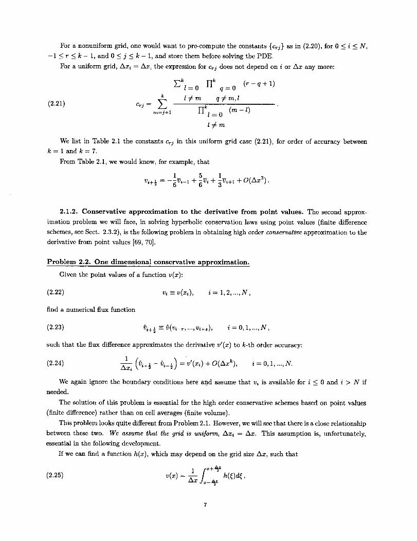
Foranonuniformgrid,onewouldwantto pre-computetheconstants{ccj} asin (2.20),for0 < i < N,
-1 < r < k - 1, and 0 < j < k - 1, and store them before solving the PDE.
For a uniform grid, Ax+ = Ax, the expression for ccj does not depend on i or Ax any more:
(2.21)
E k [Ik (r - g + 1)/=0 q=O
l#m q#m,l
m=j+_ 1-Ikl= o (m - l)
l#m
We list in Table 2.1 the constants c_j in this uniform grid case (2.21), for order of accuracy between
k=l andk=7.
From Table 2.1, we would know, for example, that
1 5 1
Vi+ ½ _- --_Vi_ 1 -_- _Vi "_ _Vi+I @ O(mX3) .
2.1.2. Conservative approximation to the derivative from point values. The second approx-
imation problem we will face, in solving hyperbolic conservation laws using point values (finite differencc
schemes, see Sect. 2.3.2), is the following problem in obtaining high order conservative approximation to the
derivative from point values [69, 70].
Problem 2.2. One dimensional conservative approximation.
Given the point values of a function v(x):
(2.22) vi =- v(x+), i = 1, 2, ..., N,
find a numerical flux function
(2.23) vi+½ = _3(vi-T, ..., v++8), i = 0, 1, ..., N,
such that the flux difference approximates the derivative v'(x) to k-th order accuracy:
(2.24) 1 (fji+½__i_½)=v,(xi)+O(Axk) ' i = 0, 1,...,N.Axi
We again ignore the boundary conditions here and assume that vi is available for i < 0 and i > N if
needed.
The solution of this problem is essential for the high order conservative schemes based on point values
(finite difference) rather than on cell averages (finite volume).
This problem looks quite different from Problem 2.1. However, we will see that there is a close relationship
between these two. We assume that the grid is uniform, Ax_ = Ax. This assumption is, unfortunately,
essential in the following development.
If we can find a function h(x), which may depend on the grid size Ax, such that
1 f _+ -_2_(2.25) v(x) = _xx j___ h(_)d_,
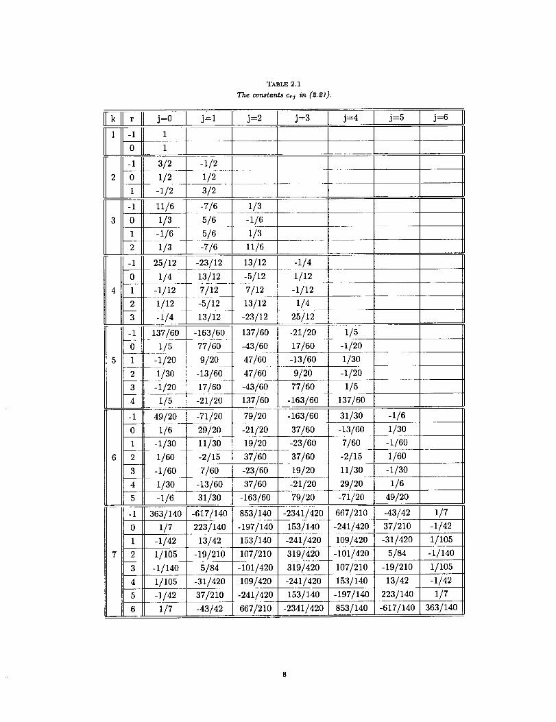
TABLE 2.1
The constants or) in (2.21).
0 1
-I
0
1
J=liJ=2 j=3 j---4
-1
0
1
2
-I
0
3/2 -1/21/2 1/2
-1/2 3/2
4 1
2
3
-1
0
5 1
2
3
4
-1
0
1
6 2
3
4
5
1
7 2
3
4
5
6
11/6 -7/61/3 5/6
-1/6 5/6
1/3 -7/6
137/6o
115
49/20
1/6
-1/30
1/60
-1/60
1/3o-1/6
-1 363/140
o 117-1/42
1/105
-I/140
1/lO5-i/421/7
25112 -23/12
114 13/12-1/12 7/12
1/12 -5/12
-1/4 13112
-163160
1/5 77/60
-1/20 9/20
1/30 -13160
-1/20 17/60
-21/20
-71/2o
29/2011130
-2/15
7/60
-13/60
31/3o
1/3
-1/6
1/311/6
13/12 -I/4
1/12-5/12711213/12 1/4
-23/12
137/60
-43/60
47/60
47/60
-43/60
137/60
79/20
-21/20
19120
-1/12
37/60
-23/60
25/12
-21/20 1/5
17/60 -1/20
-13/60 1/30
9/20 -1/20
77/60 1/5
-163/60 137/60
-163/60 31/3037/60 -13/60-23/60 7/6037t60 -2/15
19/20 11/30
-21/20 29/2079/20 -71/20
j=5
223/140 -197/140
-1/6
1/30
-1/60
1/60
-1/30
j=6
37/60 1/6
-163/60 49/20
-617/140 853/140 -2341/420 667/210 -43/42 1/7
37/210 -1/42153/140
-241/420
319/420
319/420
-2411420
109/420
-101/420
107/210
153/140
-1971140
853/140
13/42 153/140
-19/210 107/210
5/84 -i01/420
-31/420 109/420
37/210 -241/420
-43/42 667/210
-241/420
153/140
-31/420
5/84
-19/210
13/42
223/140
-617/140-23411420
1/105
-II140
1/lO5
-1/42
1/7
363/140
thenclearly
henceall weneedto dois to use
(2.26) _)i+½= h(xi+½) + O(Axk)
to achieve (2.24). We note here that it would look like an O(Ax k+l) term in (2.26) is needed in order to get
(2.24), due to the Ax term in the denominator. However, in practice, the O(Ax k) term in (2.26) is usually
smooth, hence the difference in (2.24) would give an extra O(Ax), just to cancel the one in the denominator.
It is not easy to approximate h(x) via (2.25), as it is only implicitly defined there. However, we notice
that the known function v(x) is the cell average of the unknown function h(z), so to find h(x) we just need
to use the reconstruction procedure described in Sect. 2.1.1. If we take the primitive of h(x):
(2.27)
then (2.25) clearly implies
(2.28)
/H(x) = h(_)d_ ,oc
i /x,+½ iH(x,+½)= _ h(_ld_=Ax Z vj.j=-c_ "x__ ½ j=-c_
Thus, given the point values {vj }, we "identify" them as cell averages of another function h(x) in (2.25),
then the primitive function H(x) is exactly known at the cell interfaces x = xi+ ½. We thus use the same
reconstruction procedure described in Sect. 2.1.1, to get a k-th order approximation to h(xi+½) , which is
then taken as the numerical flux _)i+ ½ in (2.23).
In other words, if the "stencil" for the flux _)i+½ in (2.23) is the following k points:
(2.29) Xi-r, ..., xi+s ,
where r + s = k - 1, then the flux _i+½ is expressed as
k--1
(2.3o) ½= jv _r+j,j=O
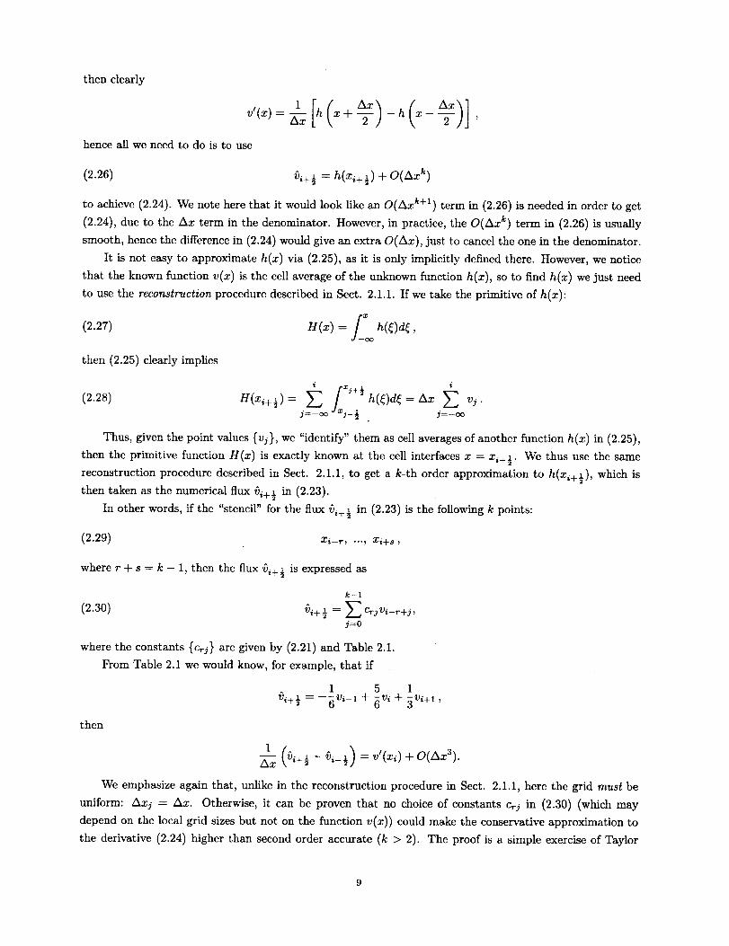
where the constants {c_j} are given by (2.21) and Table 2.1.
Prom Table 2.1 we would know, for example, that if
1 5 1?)i+½ = --_Vi-1 q- _Vi "q- _Vi+I ,
then
1 @,+}_¢)i_½)=v,(xi)+O(Axa).Ax
We emphasize again that, unlike in the reconstruction procedure in Sect. 2.1.1, here the grid must be
uniform: Axj = Ax. Otherwise, it can be proven that no choice of constants c_j in (2.30) (which may
depend on the local grid sizes but not on the function v(x)) could make the conservative approximation to
the derivative (2.24) higher than second order accurate (k > 2). The proof is a simple exercise of Taylor
expansions.Thus,thehighorderfinitedifference(thirdorderandhigher)discussedin theselecturenotescanapplyonlyto uniformorsmoothlyvaryinggrids.
Becauseofthisequivalenceofobtainingaconservativeapproximationto thederivative(2.23)-(2.24)andthereconstructionproblemdiscussedin Sect.2.1.1,wewillonlyneedto considerthereconstructionproblemin thefollowingsections.
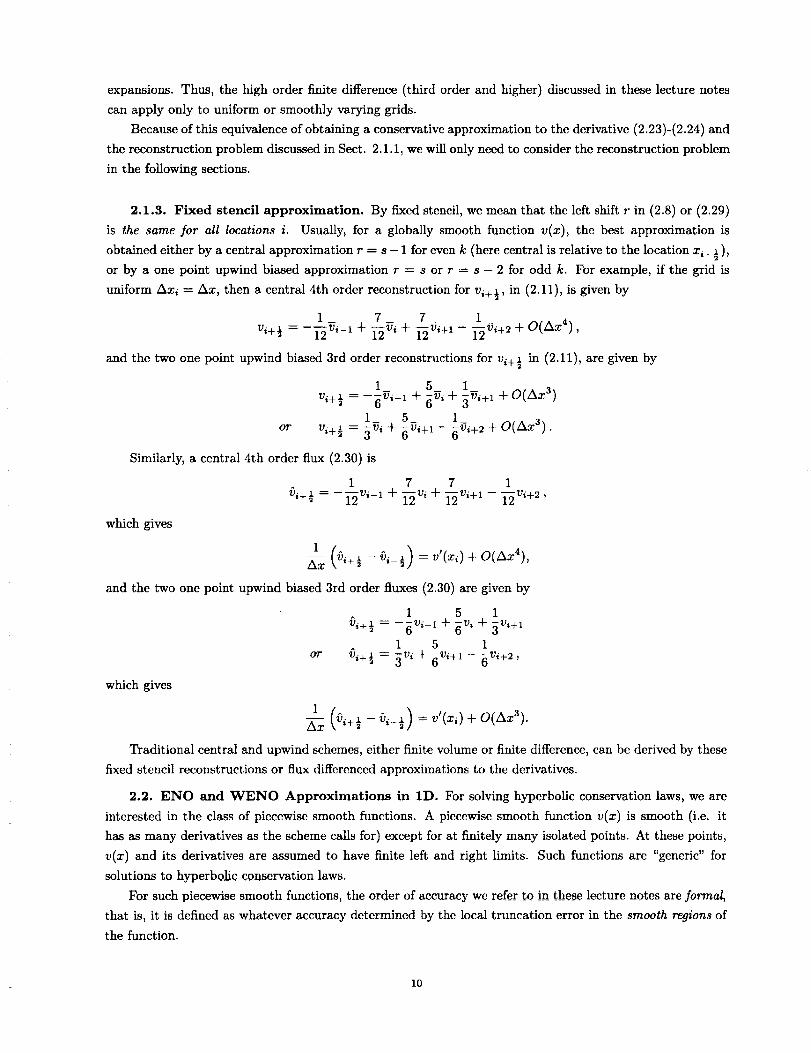
2.1.3. Fixed stencil approximation. By fixed stencil, we mean that the left shift r in (2.8) or (2.29)
is the same for all locations i. Usually, for a globally smooth function v(x), the best approximation is
obtained either by a central approximation r ----s - 1 for even k (here central is relative to the location xi+ ½),
or by a one point upwind biased approximation r = s or r = s - 2 for odd k. For example, if the grid is
uniform Axi ----Ax, then a central 4th order reconstruction for vi+½, in (2.11), is given by
1 7 7 1Vi+ ½ "_- --'i_i-1 "4- i'_V--/ _- i'_Vi+l -- "i-'_Vi+2 -t- O(AX4),
and the two one point upwind biased 3rd order reconstructions for vi+ ½ in (2.11), are given by
1 5 1vi+½ = -_v_-i + _i + 5_,+1 + O(Ax 3)
1 5 1
or vi+½ = 3v,--+ _i+_ - _v,+2 + O(Ax 3) •
Similarly, a central 4th order flux (2.30) is
1 7 7 I')i+½ = -_vi-1 + _vi + _vi+l - ]_vi+2,
which gives
1 ( i+½- = v'(x,)+Ax
and the two one point upwind biased 3rd order fluxes (2.30) are given by
1 5 1
_i+½ = -gvi-1 + gvi + 5vi+l1 5 1
Or Oi+ ½ = gVi + gVi+l -- gVi+2,
which gives
I @i+½ - v,-½) = v'(xi) + O(Ax3).Ax
Traditional central and upwind schemes, either finite volume or finite difference, can be derived by these
fixed stencil reconstructions or flux differenced approximations to the derivatives.
2.2. ENO and VC'ENO Approximations in 1D. For solving hyperbolic conservation laws, we are
intcrested in the class of piecewise smooth functions. A piecewise smooth function v(x) is smooth (i.e. it
has as many derivatives as the scheme calls for) except for at finitely many isolated points. At these points,
v(x) and its derivatives are assumed to have finite left and right limits. Such functions are "generic" for
solutions to hyperbolic conservation laws.
For such piecewise smooth fimctions, the order of accuracy wc refer to in these lecture notes are formal,
that is, it is defined as whatever accuracy determined by the local truncation error in the smooth regions of
the function.
10
Ix11-
0.5 I,-
01-
,.0.5I-
*1 I-/
i --
0.75
0.5
ozsI
OI
-oasI
-o.sl
.TSI
-11
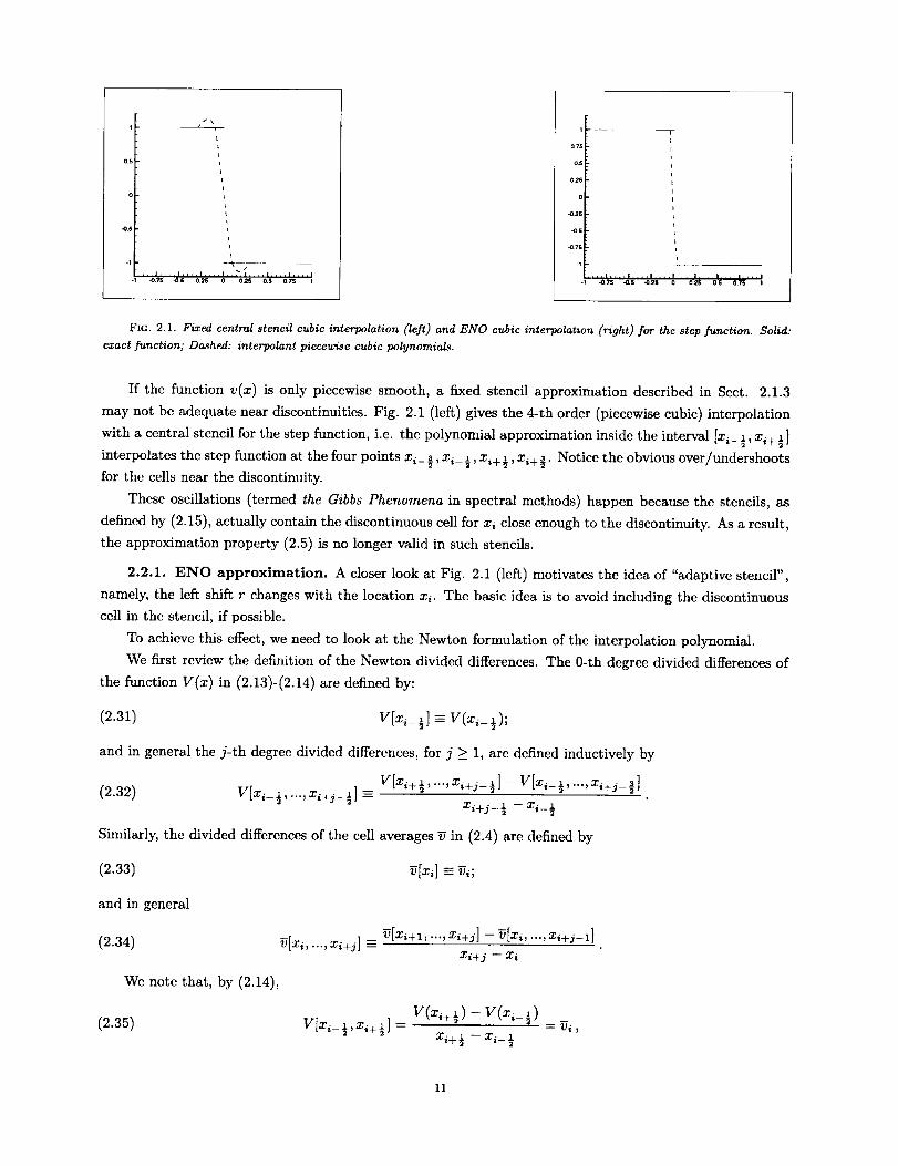
FIG. 2.1. Fixed central stencil cubic interpolation (left} and ENO cubic interpolation (right) for the step function. Solid:
exact function; Dashed: interpolant piecewise cubic polynomials.
If the hmction v(x) is only piecewise smooth, a fixed stencil approximation described in Sect. 2.1.3
may not be adequate near discontinuities. Fig. 2.1 (left) gives the 4-th order (piecewise cubic) interpolation
with a central stencil for the step function, i.e. the polynomial approximation inside the interval Ix i_ ½,xi+ ½]
interpolates the step function at the four points x,__.3, x,__l, x,___..1, xi+ ]. Notice the obvious over/undershoots
for the cells near the discontinuity.
These oscillations (termed the Gibbs Phenomena in spectral methods) happen because the stencils, as
defined by (2.15), actuMly contain the discontinuous cell for xi close enough to the discontinuity. As a result,
the approximation property (2.5) is no longer valid in such stencils.
2.2.1. ENO approximation. A closer look at Fig. 2.1 (left) motivates the idea of "adaptive stencil",
namely, the left shift r changes with the location xi. The basic idea is to avoid including the discontinuous
cell in the stencil, if possible.
To achieve this effect, we need to look at the Newton formulation of the interpolation polynomial.
We first review the definition of the Newton divided differences. The 0-th degree divided differences of
the function Y(x) in (2.13)-(2.14) are defined by:
(2.31) Y[xi_½] -- y(xi_ ½);
and in general the j-th degree divided differences, for j > 1, are defined inductively by
(2.32) V[zi- ½' "'" xi+J- ½] _ V[xi+ ½,..., xi+j_ ½] - V[x i_ ½,..., xi+j_ _]xi+__ ½ - x__ ½
Similarly, the divided differences of the cell averages _ in (2.4) are defined by
(2.33)
and in general
(2.34)
We note that, by (2.14),
(2.35)
xi+ j -- x i
V[z__½,z_+ ½] = V(z_+½) - V(zi_½) = v_,zi+ ½ - xi_ ½
11
i.e. the 0-th degree divided differences of 3 are the first degree divided differences of V(x). We can thus
write the divided differences of V(x) of first degree and higher by those of 3 of 0-th degree and higher, using
(2.35) and (2.32).
The Newton form of the k-th degree interpolation polynomial P(x), which interpolates V(x) at the k + 1
points (2.15), can be expressed using the divided differences (2.31)-(2.32) by
k j--1
j=O
We can take the derivative of (2.36) to get p(x) in (2.16):
k j-1
(2.37) p(x)---- _Y[xi_r_½,...,xi_r+j_½] Zj=l m:0
m=0
j-1
1=0
l _tm
Notice that only first and higher degree divided differences of V(x) appear in (2.37). Hence by (2.35), we
can express p(x) completely by the divided differences of 3, without any need to reference V(x).
Let us now recall an important property of divided differences:
(2.38) V[x i_ ½,..., xi+j_ 3] -- j[ ,
for some _ inside the stencil: x i_ ½ < _ < xi+ j_ ½, as long as the function V(x) is smooth in this stencil. If
V(x) is discontinuous at some point inside the stencil, then it is easy to verify that
(1)(2.39) V[xi_½,...,xi+j_½] = 0 _ .
Thus the divided difference is a measurement of the smoothness of the function inside the stencil.
We now describe the ENO idea by using (2.36). Suppose our job is to find a stencil of k + 1 consecutive
points, which must include x__ ½ and x,+ ½, such that V(x) is "the smoothest" in this stencil comparing with
other possible stencils. We perform this job by breaking it into steps, in each step we only add one point to
the stencil. Wc thus start with the two point stencil
(2.40) 2(i) = ½,x,+ ½),
where we have used S to denote a stencil for the primitive function V. Notice that the stencil S for V has
a corresponding stencil S for _ through (2.35), for example (2.40) corresponds to a single cell stencil
s(i) = {_,,,}
for 3. The linear interpolation on the stencil $2(i) in (2.40) can be written in the Newton form as
P'(x)= + x,+½](x-
At the next step, we have only two choices to expand the stencil by adding one point: we can either add the
left neighbor x__ ], resulting in the following quadratic interpolation
12
or add the right neighbor x_+ ], resulting in the following quadratic interpolation
We note that the deviations from Pl(x) in (2.41) and (2.42), are the same function
multiplied by two different constants
(2.43) V[xi_],x,_½,xi+½], and V[xi_½,x,+½,xi+]].
These two constants are the two second degree divided differences of V(x) in two different stencils. We
have already noticed before, in (2.38) and (2.39), that a smaller divided difference implies the function is
"smoother" in that stencil. We thus decide upon which point to add to the stencil, by comparing the two
relevant divided differences (2.43), and picking the one with a smaller absolute value. Thus, if
(2.44) V[x 3,x. ,,x-,l] < V[xi_ xi+]]t ,-_ =-_ =+_Jl ½'xi+½' '
we will take the 3 point stencil as
otherwise, we will take
$3(i) = {x,__,zi_½,z_+½};
_3(i) = {z__½,x_+½,z_+_}.
This procedure can be continued, with one point added to the stencil at each step, according to the
smaller of the absolute values of the two relevant divided differences, until the desired number of points in
the stencil is reached.
We note that, for the uniform grid case Ax_ = Ax, there is no need to compute the divided differences
as in (2.32). We should use undivided differences instead:
(2.45)
(see (2.35)), and
V < x,__1,z_l,T: >= Y[x__½,z_+½] = v,
(2.46)
V < xi_½, ...,xi+j+ ½ > = V < xi+½,...,xi+j+ ½ > -V < x__½, ...,xi+j_ ½ >,
j>l.
The Newton interpolation formulae (2.36)-(2.37) should also be adjusted accordingly. This both saves com-
putational time and reduces round-off effects.
The FORTRAN program for this ENO choosing process is very simple:
* assuming the m-th degree divided (or undivided) differences
* of V(x), with x_i as the left-most point in the arguments,
* are stored in V(i,m), also assuming that "is" is the
* left-most point in the stencil for cell i for a k-th
* degree polynomial
13
is=ido m=2,k
if(abs (V(is-l,m)). it. abs (V(is,m))) is=is-1
enddo
Once the stencilS(i),hence S(i),in (2.8)isfound, one could use (2.11),with the prestoredvalues of
the constantscrj,(2.20)or (2.21)Ito compute the reconstructedvaluesat the cellboundary. Or, one could
use (2.30)to compute the fluxes.An alternativeway isto compute the valuesor fluxesusing the Newton
form (2.37)directly.The computational cost isabout the same.
We summarize the ENO reconstructionprocedure inthe following
Procedure 2.1. 1D ENO reconstruction.
Given the cell averages {_,} of a function v(x), we obtain a piecewise polynomial reconstruction, of
degree at most k - 1, using ENO, in the following way:
1. Compute the divided differences of the primitive function V(x), for degrees 1 to k, using _, (2.35)
and (2.32).
If the grid is uniform Axi = Ax, at this stage, undivided differences (2.45)-(2.46) should be computed
instead.
2. In cell I_, start with a two point stencil
$_(i) = {x,_½,x,+½}
for V(x), which is equivalent to a one point stencil,
sl(0 = {z,}
for _.
3. For l ----2, ..., k, assuming
s,(o = {xj÷½,...,x_÷__½}
is known, add one of the two neighboring points, xj_ ½ or xj+t+ ½, to the stencil, following the ENO
procedure:
• If
(2.47) < l,
add x j_ ½ to the stencil St (i) to obtain
_,+1(i) = {__½,...,z_+__½};
• Otherwise, add xj+l+ ½ to the stencil St(i) to obtain
_+_(i) = {x_+½,..., x_+t+½}.
4. Use the Lagrange form (2.19) or the Newton form (2.37) to obtain pi(x), which is a polynomial of
degree at most k - 1 in Ii, satisfying the accuracy condition (2.5), as long as v(x) is smooth in Ii.
We could use pi(x) to get the approximations at the cell boundaries:
vj½ = p,(x,+½), v,+½= p,(x,_½).
14
However,it isusuallymoreconvenient,whenthestencilisknown,to use(2.10),with c_j defined
by (2.20) for a nonuniform grid, or by (2.21) and Table 2.1 for a uniform grid, to compute an
approximation to v(x) at the cell boundaries.
For the same piecewise cubic interpolation to the step function, but this time using the ENO procedure
with a two point stencil S2(i) = {x__½,x_+½} in the Step 2 of Procedure 2.1, we obtain a non-oscillatory
interpolation, in Fig. 2.1 (right).
For a piecewise smooth function V(x), ENO interpolation starting with a two point stencil S2(i) =
{x,_½, x_+½ } in the Step 2 of Procedure 2.1, as was shown in Fig. 2.1 (right), has the following properties
[39]:1. The accuracy condition
Pi(x) = Y(x) -4-O(Axk+l), x E I_
is valid for any cell Ii which does not contain a discontinuity.
This implies that the ENO interpolation procedure can recover the full high order accuracy right up
to the discontinuity.
2. P_(x) is monotone in any cell Ii which does contain a discontinuity of V(x).
3. The reconstruction is TVB (total variation bounded). That is, there exists a function z(x), satisfying
z(x) = Pi(x) + O(Axk+l), x E I_
for any cell Ii, including those cells which contain discontinuities, such that
TV(z) <_ TV(V).
Property 3 is clearly a consequence of Properties 1 and 2 (just take z(x) to bc V(x) in the smooth cells
and take z(x) to be P_(x) in the cells containing discontinuities). It is quite interesting that Property 2 holds.
One would have expected trouble in those "shocked cells", i.e. cells Ii which contain discontinuities, for ENO
would not help for such cases as the stencil starts with two points already containing a discontinuity. We
will give a proof of Property 2 for a simple but illustrative case, i.e. when V(x) is a step function
[
= 0, • _<0;V(x)( 1, x>0.
and the k-th degree polynomial P(x) interpolates V(x) at k + 1 points
containing the discontinuity
z½ < z] < ... < zk+½
xjo_ ½ < 0 < Xjo + ½
for some j0 between 1 and k. For any interval which does not contain the discontinuity 0:
(2.48) [x¢_½, xj+ ½], j #j0,
we have
P(xj_½) = V(xj_½) = V(xj+½) = P(xi+½),
15
hence there is at least one point _j in between, xj_½ < _j < xj+½, such that pr(_j) _ 0. This way we can
find k - 1 distinct zeroes for P'(x), as there are k - 1 intervals (2.48) which do not contain the discontinuity
0. However, PP(x) is a non-zero polynomial of degree at most k - 1, hence can have at most k - 1 distinct
zeroes. This implies that P'(x) does not have any zero inside the shocked interval [xjo_½, Xjo+½], i.e. P(x)
is monotone in this shocked interval. This proof can be generalized to a proof for Property 2 [39].
2.2.2. WENO approximation. In this subsection we describe the recently developed WENO (weighted
ENO) reconstruction procedure [53, 43]. WENO is based on ENO, of course. For simplicity of presentation,
in this subsection we assume the grid is uniform, i.e. Axi ----Ax.
As we can see from Sect. 2.2.1, ENO reconstruction is uniformly high order accurate right up to the
discontinuity. It achieves this effect by adaptively choosing the stencil based on the absolute values of divided
differences. However, one could make the following remarks about ENO reconstruction, indicating rooms
for improvements:
1. The stencil might change even by a round-off error perturbation near zeroes of the solution and its
derivatives. That is, when both sides of (2.47) are near 0, a small change at the round off level
would change the direction of the inequality and hencc the stencil. In smooth regions, this "free
adaptation" of stencils is clearly not necessary. Moreover, this may cause loss of accuracy when
applied to a hyperbolic PDE [63, 67].
2. The resulting numerical flux (2.23) is not smooth, as the stencil pattern may change at neighboring
points.
3. In the stencil choosing process, k candidate stencils arc considered, covering 2k - 1 cells, but only
one of the stencils is actually used in forming the reconstruction (2.10) or the flux (2.30), resulting in
k-th order accuracy. If all the 2k - 1 cells in the potential stencils are used, one could get (2k - 1)-th
order accuracy in smooth regions.
4. ENO stencil choosing procedure involves many logical "if" structures, or equivalcnt mathematical
formulae, which are not very efficient on certain vector computers such as CRAYs (however they are
friendly to parallel computers).
There have been attempts in the literature to remedy the first problem, the "free adaptation" of stencils.
In [28] and [67], the following "biasing" strategy was proposed. One first identity a "preferred" stencil
(2.49) S_e! (i) = {x,_r+ 3' .... xi-r+k+ ½}'
which might be central or one-point upwind. One then replaces (2.47) by
vlx _½, ,x. _½11<b vLx.½, I,if
x3+½ > xi__+ ½,
i.e. if the left-most point xj+½ in the current stencil S_(i) has not reached the left-most point x___+½ of the
preferred stencil Sm-_l(i ) in (2.49) yet; otherwise, if
one replaces (2.47) by
z_+½ <xi__+ ½,
b V[xj_½,...,xj+t_½] < V[xj+½,...,xj+l+½] •
16
Here,b > 1 is the so-called biasing parameter. Analysis in [67] indicates a good choice of the parameter
b -- 2. The philosophy is to stay as close as possible to the preferred stencil, unless the alternative candidate
is, roughly speaking, a factor b > 1 better in smoothness.
WENO is a more recent attempt to improve upon ENO in these four points. The basic idea is the
following: instead of using only one of the candidate stencils to form the reconstruction, one uses a convex
combination of all of them. To be more precise, suppose the k candidate stencils
(2.50) st(i) = {x,_r,..., x,_r+__l}, r = 0,...,k - 1
produce k different reconstructions to the value vi+ ½, according to (2.11),
k-1
(2.51) • (r)vi+ ½ = E c_j_i-r+j, r = 0, ..., k - 1,j=0
W-ENO reconstruction would take a convex combination of all v!r)i defined in (2.51) as a new approximation
to the cell boundary value v(xi+½):
k-1
x--" (r)(2.52) v_+ ½ = L WrVi+ ½"
r=O
Apparently, the key to the success of WENO would be the choice of the weights wr. We require
k-1
(2.5a) _r _>0, _r = 1r=O
for stability and consistency.
If the function v(x) is smooth in all of the candidate stencils (2.50), there are constants dr such that
k--1
x--" d (r)(2.54) vi+ ½ = _ rVi+ ½ = V(Xi+l ) + O(Ax2k-I).
r=0
For example, dr for 1 < k < 3 are given by
do = 1, k = 1;2 1
do = g, dl 3' k = 2;
3 3 1
do = i-6' dl = g, d2 = i-0'
We can see that dr is always positive and, due to consistency,
k-1
(2.55) _ dr = 1.r=0
In this smooth case, we would like to have
k_3.
(2.56) wr _-- dr -1- O(Axk-1), r = O, ..., k - 1,
which would imply (2k - 1)-th order accuracy:
k-1
(2.57) x-, (r) = v(x_+½)+ o(Ax 2k-1)vi+½= ?_.,_vi+ ½r=0
17
becausek-1 k-I k-1
WrVi+½ - 2..,arVi+½ \ i+½ v(xi+½r=0 r=0 r=0
k-1
= EO(Axk-1)O(Axk) _- O(Ax2k-1)
r=0
where in the first equality we used (2.53) and (2.55).
When the function v(x) has a discontinuity in one or more of the stencils (2.50), we would hope the
corresponding weight(s) wr to be essentially 0, to emulate the successful ENO idea.
Another consideration is that the weights should be smooth functions of the cell averages involved. In
fact, the weights designed in [43] and described below are C _°.
Finally, we would like to have weights which are computationally efficient. Thus, polynomials or rational
functions are preferred over exponential type functions.
All these considerations lead to the following form of weights:
0/r
(2.58) Wr = k-1 'Es=O C_s
with
r = 0,...,k- 1
dr(2.59) _ = (e +/3r) 2"
Here e > 0 is introduced to avoid the denominator to become 0. Wc take e = 10 -s in all our numerical
tests [43]. /3r are the so-called "smooth indicators" of the stencil S_(i): if the function v(x) is smooth in the
stencil St(i), then
3_ = 0(Ax2),
but if v(x) has a discontinuity inside the stencil St(i), then
3r = o(1).
Translating into the weights wr in (2.58), we will have
_r = o(1)
when the function v(x) is smooth in the stencil St(i), and
o;r = O(Az 4)
if v(x) has a discontinuity inside the stencil St(i). Emulation of ENO near a discontinuity is thus achieved.
One also has to worry about the accuracy requirement (2.56), which must be checked when the specific
form of the smooth indicator/3r is given. For any smooth indicator fl_, it is easy to see that the weights
defined by (2.58) satisfies (2.53). To satisfy (2.56), it sutfices to have, through a Taylor expansion analysis:
(2.60) fir = D (1 + O(Axk-1)), r = 0, ..., k - 1,
where D is a nonzero quantity independent of r (but may depend on Ax).
18
As we have seen in Sect. 2.2.1, the ENO reconstruction procedure chooses the "smoothest" stencil by
comparing a hierarchy of divided or undivided differences. This is because these differences can be used
to measure the smoothness of the function on a stencil, (2.38)-(2.39). In [43], after extensive experiments,
a robust (for third and fifth order at least) choice of smooth indicators/3r is given. As we know, on each
stencil Sr (i), we can construct a (k- 1)-th degree reconstruction polynomial, which if evaluated at x --- x_+ 5'
renders the approximation to the value v(xi+ 5 ) in (2.51). Since the total variation is a good measurement for
smoothness, it would be desirable to minimize the total variation for this reconstruction polynomial inside
Ii. Consideration for a smooth flux and for the role of higher order variations leads us to the following
measurement for smoothness: let the reconstruction polynomial on the stencil Sr(i) be denoted by pr(x), we
define
(2.61) fl_=_'+½/=l ,_½ Ax2t-I (Otpr(x))2\O'x dx.
The right hand side of (2.61) is just a sum of the squares of scaled L 2 norms for all the derivatives of the
interpolation polynomial p_(x) over the interval (x i_ 5' x_+½). The factor Ax 21-1 is introduced to remove
any Ax dependency in the derivatives, in order to preserve self-similarity when used to hyperbolic PDEs
(Sect. 2.3).
We remark that (2.61) is similar to but smoother than the total variation measurement based on the L 1
norm. It also renders a more accurate WENO scheme for the case k -- 2 and 3.
When k = 2, (2.61) gives the following smoothness measurement [53, 43]:
Z0 = (vi+l -
Zl = - v,-1) 2•(2.62)
For k -- 3, (2.61) gives [43]:
(2.63)
13Z0=
13
=13
2Viq-1 + Vi+2) 2 -']'- _(3_i - 4Vi+l -[- vi+2) 2 ,
1_ )2-- 2Vi "q- Vi+l) 2 + _(Vi-1 -- Vi+l ,
1- 2v___ + _)2 + _(v_-2 - 4___ + 3vd 2 .
We can easily verify that the accuracy condition (2.60) is satisfied, even near smooth extrema [43]. This
indicates that (2.62) gives a third order WENO scheme, and (2.63) gives a fifth order one.
Notice that the discussion here has a one point upwind bias in the optimal linear stencil, suitable for
a problem with wind blowing from left to right. If the wind blows the other way, the procedure should be
modified symmetrically with respect to xi+ 5"
In summary, we have the following WENO reconstruction procedure:
Procedure 2.2. 1D WENO reconstruction.
Given the cell averages {_i} of a function v(x), for each cell/_, we obtain upwind biased (2k - 1)-th
order approximations to the function v(x) at the cell boundaries, denoted by v+- ½ and v_+5, in the following
way:
1. Obtain the k reconstructed values v(_)_, of k-th order accuracy, in (2.51), based on the stencilsi-}-_
(2.50), for r = 0, ..., k - 1;
Also obtain the k reconstructed values v (r) of k-th order accuracy, using (2.10), again based on
the stencils (2.50), for r = 0, ..., k - 1;
19
2. Find the constants dr and dr, such that (2.54) and
k--1
vi_ _] = E ;arVi-(r)½= v(xi_½) + O(Az 2k-1 )
are valid. By symmetry,
C[r _ dk-l-r.
3. Find the smooth indicators 3r in (2.61), for all r = 0, ..., k - 1. Explicit formulae for k - 2 and
k = 3 are given in (2.62) and (2.63) respectively.
4. Form the weights w_ and &_ using (2.58)-(2.59) and
wr = k-1 , &r ---- r ----0, ..., k - 1.E_=o a_, (_+ 3r)2'
5. Find the (2k - 1)-th order reconstruction
k-1 k--1
,-,(2.64) v_+ ½ ----L wrv_+ ½..... •r=0 r=0
We can obtain weights for higher orders of k (corresponding to seventh and higher order _:ENO schemes)
using the same recipe. However, these schemes of seventh and higher order have not been extensively tested
yet.
2.3. ENO and WENO Schemes for 1D Conservation Laws. In this section we describe the ENO
and W'ENO schemes for 1D conservation laws:
(2.65) =_(_,t) + f_(u(x,t)) = o
equipped with suitable initial and boundary conditions.
We will concentrate on the discussion of spatial discretization, and will leave the time variable t contin-
uous (the method-of-lines approach). Time discretizations will be discussed in Sect. 4.2.
Our computational domain is a < x < b. We have a grid defined by (2.1), with the notations (2.2)-(2.3).
Except for in Sect. 2.3.3, we do not consider boundary conditions. We thus assume that the values of the
numerical solution are also available outside the computational domain whenever they are needed. This
would be the case for periodic or compactly supported problems.
2.3.1. Finite volume formulation in the scalar case. For finite volume schemes, or schemes based
on cell averages, we do not solve (2.65) directly, but its integrated version. We integrate (2.65) over the
interval Ii to obtain
d-_(x,,t) _ 1 (f(u(xi+½,t)- f(u(x,_½,t))) ,dt Ax_
(2.66)
where
(2.67) 1 ix,+½ u(_,t) d__(x,, t) - _. _,-
is the cell average. We approximate (2.66) by the following conservative scheme
(2.68) d_i(t) 1
2O
where ui (t) is the numerical approximation to the cell average _(xi, t), and the numerical flux ]i+ ½ is definedby
(2.70)
2. Engquist-Osher flux:
with the values u_+½ obtained by the ENO reconstruction Procedure 2.1, or by the WENO reconstructionProcedure 2.2.
The two argument function h in (2.69) is a monotone flux. It satisfies:
• h(a, b) is a Lipschitz continuous function in both arguments;
• h(a, b) is a nondecreasing function in a and a nonincreasing function in b. Symbolically h(T, _);
• h(a, b) is consistent with the physical flux f, that is, h(a, a) = f(a).
Examples of monotone fluxes include:
1. Godunov flux:
h(a, b) = [ mina<_<b f(u) if a < b
[ maxb_<_,<a f(u) if a > b '
(2.71)
3. Lax-Friedrichs flux:
° fobh(a, b) = max(/'(u), O)du + min(f'(u), O)du + f(O).
h(a, b) = 1 [f(a) +/(b) - - a)](2.72)
where a = max_ [f'(u)l is a constant. The maximum is taken over the relevant range of u.
We have listed the monotone fluxes from the least dissipative (less smearing of discontinuities) to the most.
For lower order methods (order of reconstruction is 1 or 2), there is a big differencc between results obtained
by different monotone fluxes. However, this difference becomes much smaller for higher order reconstructions.II 2
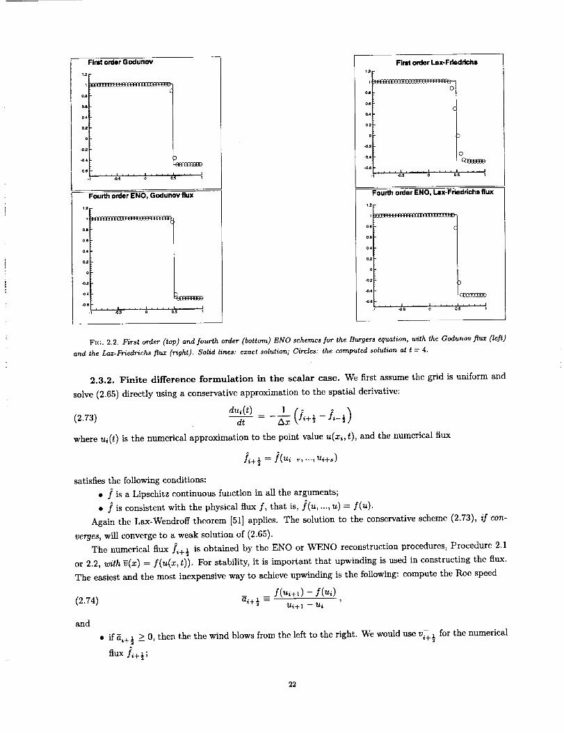
In Fig. 2.2, we plot the results of a right moving shock for the Burgers' equation (f(u) = -_- in (2.65)),
with first order reconstruction using Godunov and Lax-Friedrichs monotone fluxes (top), and with fourth
order ENO reconstruction using Godunov and Lax-Friedrichs monotone fluxes (bottom). We can clearly see
that, while the Godunov flux behaves much better for the first order scheme, the two fourth order ENO
schemes behave similarly. We thus use the simple and inexpensive Lax-Friedrichs flux in most of our highorder calculations.
We remark that, by the classic Lax-Wendroff theorem [51], the solution to the conservative scheme
(2.68), if converges, will converge to a weak solution of (2.65).
In summary, to build a finite volume ENO scheme (2.68), given the cell averages {_} (we will often
drop the explicit reference to the time variable t), we proceed as follows:
Procedure 2.3. Finite volume 1D scalar ENO and WENO.
1. Follow the Procedure 2.1 in Sect. 2.2.1 for ENO, or the Procedure 2.2 in Sect. 2.2.2 for WENO, to
obtain the k-th order reconstructed values uY_+_land u++_½for all i;
2. Choose a monotone flux (e.g., one of (2.70) to (2.72)), and use (2.69) to compute the flux ]i+½ forall i;
3. Form the scheme (2.68).
Notice that the finite volume scheme can be applied to arbitrary nonuniform grids.
21
Find order Godunov
,.2p
Oil-
0.61-
0.4 I.-
021-
01-
-021-
.04 _- ::)
.0.0 I-
-, .... IS .... ; .... O'.S .... ;
Fourth order ENO, Godunov flux
oJl-
o.et.
04 I-
o.2F
oF
-04 I.
_.e [-
.... .0.s; .... ol , . , ' o$1. .... II
Find order Lax-Frledrich$
ooil-
o.61-
o,4 I-
o21-
oD- )
-o21-
-o.4 r,-. 0
-c_mm.0.6 I-
-1 0.5 1
Fourth onclerENO, Lax-Friedrichs flux
1.2 -
1
OJ
OJ
0.4
02
0
-02)
-O4OE_B_BE_
.0.$.... i . . . i .... i .... i
-0.5 0 0.5 '
FIC. 2.2. First order (top) and fourth order (bottom) ENO schemes for the Burgers equation, with the Godunov flux (left)
and the Lax-b_iedrichs flux (right). Solid lines: exact solution; Circles: the computed solution at t = 4.
2.3.2. Finite difference formulation in the scalar case. We first assume the grid is uniform and
solve (2.65) directly using a conservative approximation to thc spatial derivative:
(2.73)dt Ax
where ui(t) is the numerical approximation to the point value u(x_, t), and the numerical flux
L+½ =/(u,-r, ..., _,+,)
satisfies the following conditions:
• ] is a Lipschitz continuous function in all the arguments;
• ] is consistent with the physical flux f, that is, ](u .... , u) = f(u).
Again the Lax-Wendroff theorem [51] applies. The solution to the conservative scheme (2.73), /f con-
verges, will Converge to a weak solution of (2.65).
The numerical flux ]_+½ is obtained by the ENO or WENO reconstruction procedures, Procedure 2.1
or 2.2, with _(x) = f(u(x, t)). For stability, it is important that upwinding is used in constructing the flux.
The easiest and the most inexpensive way to achieve upwinding is the following: compute the Roe speed
_/(_i+1) -/(_i)(2.74) hi+½ = ,
Ui-)-I -- Ui
and
• ff _,+ ½ > O, then the the wind blows from the left to the right. We would use v_+ ½ for the numerical^
flux fi+½;
22
• if ai+½ < 0, then the wind blows from the right to the left. We would use v._] for the numerical^
flux fi+½"
This produces the Roe scheme [62] at the first order level. For this reason, the ENO scheme based on this
approach was termed "ENO-Roe" in [70].
In summary, to build a finite difference ENO scheme (2.73) using the ENO-Roe approach, given the point
values {ui} (we again drop the explicit reference to the time variable t), we proceed as follows:
Procedure 2.4. Finite difference 1D scalar ENO- and WENO-Roe.
1. Compute the Roe speed _,+½ for all i using (2.74);
2. Identify Vi = f(u_) and use the ENO reconstruction Procedure 2.1 or the WENO reconstruction
Procedure 2.2, to obtain the cell boundary values v- 1 if _i+½ > 0, or v +,+_ - i+½ if_i+½ < 0;
3. If the Roe speed at xi+ ½ is positive
then take the numerical flux as:
otherwise, take the the numerical flux as:
a- +½_>o,
= v \½;
= v++½;
4. Form the scheme (2.73).
One disadvantage of the ENO-Roe approach is that entropy violating solutions may be obtained, just
like in the first order ROe scheme case. For example, if ENO-Roe is applied to the Burgers equation
with the following initial condition
u(x,O)= _ -1, if x<0,
L 1, ifx >_ 0,
it will converge to the entropy violating expansion shock:
u(x,t)=_ -1, if x<0,
t 1, ifx _> 0.
Local entropy correction could be used to remedy this [70]. However, it is usually more robust to use a
global "flux splitting":
(27 )
where
(2.76)
f(u) = f+(u) + f-(u)
df+(u) > O, df- (u) < O.du du -
We would need the positive and negative fluxes f+ (u) to have as many derivatives as the order of the scheme.
This unfortunately rules out many popular fluxes (such as those of van Leer [79] and Osher [58]) for high
order methods in this framework.
23
Thesimplestsmoothsplittingis theLax-Friedrichssplitting:
(2.77) f+ (u) --- l (f(u) • _u)
where _ is again taken as _ = max_ If'(u)l over the relevant range of u.
We note that there is a close relationship between a flux splitting (2.75) and a monotone flux (2.69). In
fact, for any flux splitting (2.75) satisfying (2.76),
(2.78) h(a, b) = f+(a) + f-(b)
is clearly a monotone flux. However, not every monotone flux can be written in the flux split form (2.75).
For example, the Codunov flux (2.70) cannot.
With the flux splitting (2.75), we apply the the ENO or WENO reconstruction procedures, Procedure
2.1 or 2.2, with _(x) = f+(u(x, t)) and _(x) = f-(u(x, t)) separately, to obtain two numerical fluxes ]+½^
and fi+ ½' and then sum them to get the numerical flux ]_+ ½.In summary, to build a finite difference (FD) ENO or WENO scheme (2.73) using the flux splitting
approach, given the point values (u,}, we proceed as follows:
Procedure 2.5. FD 1D scalar flux splitting ENO and WENO.
1. Find a smooth flux splitting (2.75), satisfying (2.76);
2. Identify _, -- f+ (u_) and use the ENO or WENO reconstruction procedure, Procedure 2.1 or 2.2, to
obtain the cell boundary values v_+½ for all i;
3. Take the positive numerical flux as
= v_+½;
4. Identify V_ = f-(ui) and use the ENO or WENO reconstruction procedures, Procedure 2.1 or 2.2,
to obtain the cell boundary values v_½ for all i;
5. Take the negative numerical flux as
]_½ = v++½;
6. Form the numerical flux as
i÷½ ^+ ^= fi÷½ + fL½;
7. Form the scheme (2.73).
We remark that the finite difference scheme in this section and the finite volume scheme in Sect. 2.3.1
are equivalent for one dimensional, linear PDE with constant coefficients: the only difference is in the initial
conditions (one uses point values and the other uses cell averages of the exact initial condition). Notice
that the schemes are still nonlinear in this case. However, this equivalence does not hold for a nonlinear
PDE. Moreover, we will see later that there are significant differences in efficiency of the two approaches for
multidimensional problems.
In the following we test the accuracy of the fifth order finite difference WENO schemes on the linear
equation:
u_ ÷ ux = O, -l<x<l
u(x, O) = uo(x) periodic.
24
Method
WENO-5
CENTRAl5
TABLE 2.2
Accuracy on u_ + ux = 0 with uo(x) = sin(_rx).
N
10
20
40
80
160
320
10
20
40
80
160
320
Lo_ error Lo_ order L1 error L1 order
2.98e-2
1.45e-3
4.58e-5
1.48e-6
4.41e-8
1.35e-9
4.98e-3
1.60e-4
5.03e-6
1.57e-7
4.91e-9
1.53e-10
4.36
4.99
4.95
5.07
5.03
4.96
4.99
5.00
5.00
5.00
1.60e-2
7.41e-4
2.22e-5
6.91e-7
2.17e-8
6.79e-10
3.07e-3
9.92e-5
3.14e-6
9.90e-8
3.11e-9
9.73e-ll
4.43
5.06
5.01
4.99
5.00
4.95
4.98
4.99
4.99
5.00
Method
WENO-5
CENTRAl5
TABLE 2.3
Accuracy on u_ + ux = 0 with uo(x) = sin4(lrx).
N
20
40
80
160
320
640
20
40
80
160
320
640
L_ error
1.08e-1
8.90e-3
1.80e-3
1.22e-4
4.37e-6
9.79e-8
5.23e-2
2.47e-3
8.32e-5
2.65e-6
8.31e-8
2.60e-9
L_ order
3.60
2.31
3.88
4.80
5.48
4.40
4.89
4.97
5.00
5.00
L1 error
4.91e-2
3.64e-3
5.00e-4
2.17e-5
6.17e-7
1.57e-8
3.35e-2
1.52e-3
5.09e-5
1.60e-6
4.99e-8
1.56e-9
L1 order
3.75
2.86
4.53
5.14
5.30
4.46
4.90
4.99
5.00
5.00
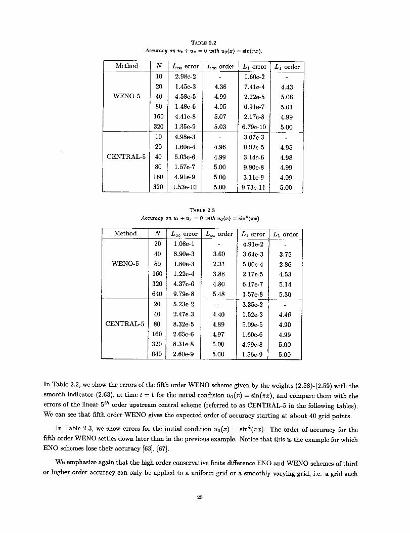
In Table 2.2, we show the errors of the fifth order WENO scheme given by the weights (2.58)-(2.59) with the
smooth indicator (2.63), at time t -- 1 for the initial condition Uo(X) = sin(Trx), and compare them with the
errors of the linear 5 th order upstream central scheme (referred to as CENTRAL-5 in the following tables).
We can see that fifth order WENO gives the expected order of accuracy starting at about 40 grid points.
In Table 2.3, we show errors for the initial condition Uo(X) = sina(lrx). The order of accuracy for the
fifth order WENO settles down later than in the previous example. Notice that this is the example for which
ENO schemes lose their accuracy [63], [67].
We emphasize again that the high order conservative finite difference ENO and WENO schemes of third
or higher order accuracy can only be applied to a uniform grid or a smoothly varying grid, i.e. a grid such
25
that asmoothtransformation
=
will result in a uniform grid in the new variable 4- Here _ must contain as many derivatives as the order of
accuracy of scheme calls for. If this is the case, then (2.65) is transformed to
+ xf(u) = 0
and the conservative ENO or WENO derivative approximation is then applied to f(u)_. It is proven in [58]
that this way the scheme is still conservative, i.e. Lax-Wendroff theorem [51] still applies.
2.3.3. Boundary conditions. For periodic boundary conditions, or problems with compact support
for the entire computation (not just the initial data), there is no difficulty in implementing boundary condi-
tions: one simply set as many ghost points as needed using either the periodicity condition or the compactness
of the solution.
Other types of boundary conditions should be handled according to their type: for reflective or symmetry
boundary conditions, one would set as many ghost points as needed, then use the symmetry/antisymmetry
properties to prescribe solution values at those ghost points. For inflow or partially inflow (e.g. a subsonic
outflow where one of the characteristic waves flows in) boundary conditions, one would usually use the
physical inflow boundary condition at the exact boundary (for example, if x½ is the left boundary and a
finite volume scheme is used, one would use the given boundary value Ub as u_ in the monotone flux at x½;
if x0 is the left boundary and a finite difference scheme is used, one would use the given boundary value Ub
as u0). Apart from that, the most natural way of treating boundary conditions for the ENO scheme is to use
only the available values inside the computational domain when choosing the stencil. In other words, only
stencils completely contained inside the computational domain is used in the ENO stencil choosing process
described in Procedure 2.1. In practical implementation, in order to avoid logical structures to distinguish
whether a given stencil is completely inside the computational domain, one could set all the ghost values
outside the computational domain to bc very large with large variations (e.g. setting u_j = (10j) 1° if
x_j, for j = 1, 2, ..., are ghost points). This way the ENO stencil choosing procedure will automatically
avoid choosing any stencil containing ghost points. Another way of treating boundary conditions is to use
extrapolation of suitable order to set the values of the solution in all necessary ghost points. For scalar
problems this is actually equivalent to the approach of using only the stencils inside the computational
domain in the ENO procedure. WENO can be handled in a similar fashion.
Stability analysis (GKS analysis [30], [76]) can be used to study the linear stability when the boundary
treatment described above is applied to a fixed s.tencil upwind biased scheme. For most practical situations
the schemes are linearly stable [3].
2.3.4. Provable properties in the scalar case. Second order ENO schemes are also TVD (total
variation diminishing), hence have at least subsequences which converge to weak solutions. There is no
known convergence result for ENO schemes of degree higher than 2, even for smooth solutions.
WENO schemes have better convergence results, mainly because their numerical fluxes are smoother. It
is proven [43] that WENO schemes converge for smooth solutions. Also, Jiang and Yu [44] have obtained an
existence proof for traveling waves for WENO schemes. This is an important first step towards the proof of
convergence for shocked cases.
Even though there are very little theoretical results about ENO or WENO schemes, in practice these
schemes are very robust and stable. We caution against any attempts to modify the schemes solely for the
26
purposeof stabilityor convergenceproofs.In [69]wegavearemarkabouta modificationof ENOschemes,whichkeepstheformaluniformhighorderaccuracyandmakesthemstableandconvergentforgeneralmultidimensionalscalarequations.Howeverit waspointedouttherethatthemodificationisnotcomputationallyuseful,hencetheconvergenceresulthaslittle value.
Theremarkin [69]is illustrativehencewereproduceit here.Westartwith a flux splitting(2.75)satisfying(2.76),andnoticethat thefirstordermonotonescheme
(2.79) dui _ 1dt AX, (f+(ui) -- f+(ui-1) q- f-(ui+l) -- f-(ui)) =-- Rl(U)i
is convergent (also for multi space dimensions). We now construct a high order ENO approximation in thc
following way: starting from the two point stencil {xi-1, xi}, we expand it into a k + 1 point stencil in an
ENO fashion using the divided differences of f+(u(x)). We then build the k-th degree polynomial P+(x)
which interpolates f+(u(x)) in this stencil. P-(x) is constructed in a similar way, starting from the two
point stencil {x,, x_+l}. The scheme is finally defined as
(2.80) du__)_= _d (P+(x) ÷ P-ix))I_=_, =- Rk(u),dt dx
This scheme is clearly k-th order accurate but is not conservative. We now denote the differcncc bctween
the high order scheme (2.80) and the first order monotone scheme (2.79) by
(2.81) D(u)i - Rk(u)_ -- Rl(u)i,
and limit it by
(2.82) Z)(u)i = _(D(u)i, MAxa),
where M > 0 and 0 < a < 1 are constants, and the capping function _ is defined by
fre(a, b) = /
%
The modified ENO scheme is then defined by
a, if lal _ b;
b, if a > b;
-b, if a < -b.
(2.83) duid--t- = Rk(u)i -- Rl(u)i + D(u)i.
We notice that, in smooth regions, the difference between the first order and high order residues, D(u),, as
defined in (2.81), is of the size O(Ax), hence the capping (2.82) does not take effect in such regions, if a < 1
or if c_ = 1 and M is large enough, when Ax is sufficiently small. This implies that the scheme (2.83) is
uniformly accurate. Moreover, since
Rk(u)_ -- Rl(u)i <_ MAx _
by (2.82), the high order scheme (2.83) shares every good property of the first order monotone scheme
(2.79), such as total variation boundcdness, entropy conditions, and convergence. From a theoretical point
of view, this is the strongest result one could possibly hope for a high order scheme. However, the mesh size
dependent limiting (2.82) renders the scheme highly impractical: the quality of the numerical solution will
depend strongly on the choice of the parameters M and a, as well as on the mesh size Ax.
27
2.3.5. Systems.Weonly consider hyperbolic m × m systems, i.e.
eigenvalues
(2.84) A1 (u) __... _< Am (u)
and a complete set of independent eigenvectors
(2.85) rl (u), ..., rm(_).
We denote the matrix whose columns are eigenvectors (2.85) by
R(u) = (rl (u), ..., rm(u))(2.86)
Then clearly
(2.87)
thc 3ocobian f'(u) has m real
n-l(u) f'(_) n(_) = A(_)
where A(u) is the diagonal matrix with A1 (u),..., Am(U) on the diagonal. Notice that the rows of R-l(u),
denotcd by 11(u), ..., lm(u) (row vectors), are left eigenvectors of f'(u):
(2.88) l,(_)f'(_) = _(_)t,(_), i = 1,..., m.
There are several ways to generalize scalar ENO or WENO schemes to systems.
The easiest way is to apply the ENO or WENO schemes in a component by component fashion. For the
finite volume (FV) formulation, this means that we make the reconstruction using ENO or WENO for each
of the components of u separately. This produces the left and right values u_+ ½ at the cell interface xi+ ½.
An exact or approximate Riemann solver, h(u_+½, u++½), is then used to build the scheme (2.68)-(2.69).
The exact Riemann solver is given by the exact solution of (2.65) with the following step function as initial
condition
{-(2.89) u(x,O) = ui+½, x < 0;
u++½, x >0.
Notice that the solution to (2.65) with the initial condition (2.89) is self-
If we denote this
evaluated at the center x = 0.
similar, that is, it is a function of the variable _ = z hence is constant along x -- 0.¥,
solution by ui+ ½, then the flux is taken as
h(u_+½,_+ ½) = I(_+ ½1.
In the scalar case, the exact Riemann solver gives the Godunov flux (2.70). Exact Riemann solver can be
obtained for many systems including the Euler equations of compressible gas, which is used very often in
practice. However, it is usually very costly to get this solution (for Euler equations of compressible gas, an
iterative procedure is needed to obtain this solution, see [74]). In practice, approximate Riemann solvers
are usually good enough. As in the scalar case, the quality of the solution is usually very sensitive to the
choice of approximate Riemann solvers for lower order schemes (first or second order), but this sensitivity
decreases with an increasing order of accuracy. The simplest approximate Riemann solver (albeit the most
dissipative) is again the Lax-Friedrichs solver (2.72), except that now the constant a is taken as
(2.90) a=m_x max I_(_)ll _ j<rn
28
where )_j (u) are the eigenvalues of the Jacobian if(u), (2.84). The maximum is again taken over the relevant
range of u.
We summarize the procedure in the following
Procedure 2.6. Component-wise FV 1D system ENO and WENO.
1. For each component of the solution _, apply the scalar ENO Procedure 2.1 or WENO Procedure
2.2 to reconstruct the corresponding component of the solution at the cell interfaces, u/_+½ for all i;
2. Apply an exact or approximate Riemann solver to compute the flux ],+½ for all i in (2.69);
3. Form the scheme (2.68).
For the finite difference formulation, a smooth flux splitting (2.75) is again needed. The condition (2.76)
now becomes that the two Jacobians
(2.91) Of+(u) Of-(u)Ou ' Ou
are still diagonalizable (preferably by the same eigenvectors R(u) as for if(u)), and have only non-negative
/ non-positive eigenvalues, respectively. We again recommend the Lax-Friedrichs flux splitting (2.77), with
given by (2.90), because of its simplicity and smoothness. A somewhat more complicated Lax-Friedrichs
type flux splitting is:
= _(f(u) -4-R(u)_R-l(u) u),f_:(u)
where R(u) and R-l(u) arc defined in (2.86), and
= diag(_l,..., Am)
where _j = maxul)_j(u)l, and the maximum is again taken over the relevant range of u. This way the
dissipation is added in each field according to the maximum size of eigenvalues in that field, not globally.
One could also use other flux splittings, such as the van Leer splitting for gas dynamics [79]. However, for
higher order schemes, the flux splitting must be sufficiently smooth in order to retain the order of accuracy.
With these flux splittings, we can again use the scalar recipes to form the finite difference scheme: just
^+ f/_ ½ component by component.compute the positive and negative fluxes fi+ ½ and
We summarize the procedure in the folIowing
Procedure 2.7. Component-wise FD 1D system ENO and WENO.
1. Find a flux splitting (2.75). The simplest example is the Lax-Friedrichs flux splitting (2.77), with
given by (2.90);
2. For each component of the solution u, apply the scalar Procedure 2.5 to reconstruct the corresponding
component of the numerical flux ]_+½ ;
3. Form the scheme (2.73).
These component by component versions of ENO and WENO schemes are simple and cost effectivc.
They work reasonably well for many problems, especially when the order of accuracy is not high (second or
sometimes third order). However, for more demanding test problems, or when the order of accuracy is high,
we would need the following more costly, but much more robust characteristic decompositions.
To explain the characteristic decomposition, we start with a simple example where f(u) = Au in (2.65)
is linear and A is a constant matrix. In this situation, the eigenvalues (2.84), the eigenvectors (2.85), and
the related matrices R, R -1 and A (2.86)-(2.87), are all constant matrices. If we define a change of variable
(2.92) v = R -1 u,
29
thenthePDE(2.65)becomesdiagonal:
(2.93) vt + Av= = 0
that is, the m equations in (2.93) are decoupled and each one is a scalar linear convection equation of the
form
(2.94) _, + _._ = O.
We can thus use the reconstruction or flux evaluation techniques for the scalar equations, discussed in
Sections 2.3.1 and 2.3.2, to handle each of the equations in (2.94). After we obtain the results, we can "come
back" to the physical space u by using the inverse of (2.92):
(2.95) u = Rv
For example, if the reconstructed polynomial for each component j in (2.93) is denoted by qi(x), then we
form
and obtain the reconstruction in the physical space by using (2.95):
(2.97) p(x) = R q(x)
The flux evaluations for the finite difference schemes can be handled similarly.
We now come to the situation where f_(u) is not constant. The trouble is that now all the matrices R(u),
R-1 (u) A(u) are dependent upon u. We must "freeze" them locally in order to carry out a similar procedure
as in the constant coefficient case. Thus, to compute the flux at the cell boundary xi+½, we would need an
approximation to the Jocobian at the middle value ui+ ½. This can be simply taken as the arithmetic mean
1
(2.98) u_+½ = _ (u, + u_+l) ,
or as a more elaborate average satisfying some nice properties, e.g. thc mean value theorem
(2.99) f(U_+l) - f(u_) = .f'(ui+½ )(ui+l - ui) .
Roe average [62] is such an example for the compressible Euler equations of gas dynamics and some other
physical systems. It is also possible to use two different one-sided Jacobians at a higher computational cost
[25].
Once we have this ui+½, we will use R(ui+½), R-I(ui+½) and A(u_+½) to help evaluating the numerical
flux at x_+½. We thus omit the notation i + 1 and still denote these matrices by R, R -1 and A, etc. Wc
then repeat the procedure described above for linear systems. The difference here being, the matrices R,
R- 1 and A are different at different locations x_+ ½, hence the cost of the operation is greatly increased.
3o
In summary,wehavethefollowingprocedures:
Procedure 2.8. Characteristic-wise FV 1D ENO and WENO
1. Compute the divided or undivided differences of the cell averages _, for all i;
2. At each fixed xi+ 3' do the following:
(a) Compute an average state ui+ 3' using either the simple mean (2.98) or a Roe average satisfying
(2.99);
(b) Compute the right eigenvectors, the left eigenvectors, and the eigenvalues of the Jacobian
f'(ui+½), (2.84)-(2.87), and denote them by
R = R(u_+½), R -1 = R-l(u_+½), A = A(ui+½);
(c) Transform all those differences computed in Step 1, which are in the potential stencil of the
ENO and WENO reconstructions for obtaining u_+½, to the local characteristic fields by using(2.92). For example,
vj = R -1 uj, j in a neighborhood of i;
(d) Perform the scalar ENO or WENO reconstruction Procedure 2.3, for each component of the
characteristic variables _, to obtain the corresponding component of the reconstruction v +i+½;
(e) Transform back into physical space by using (2.95):
u ½,+= t
3. Apply an exact or approximate Riemarm solver to compute the flux ]i+½ for all i in (2.69); then
form the scheme (2.68).
Similarly, the procedure to obtain a finite difference ENO-Roe type scheme using the local characteristic
variables is:
Procedure 2.9. Characteristic-wise FD 1D system, Roe-type.
1. Compute the divided or undivided differences of the flux f(u) for all i;
2. At each fixed xi+ 3' do the following:
(a) Compute an average state ui+½, using either the simple mean (2.98) or a Roe average satisfying
(2.99);
(b) Compute the right eigenvectors, the left eigenvectors, and the eigenvalues of the Jacobian
f'(u_+½), (2.84)-(2.87), and denote them by
R = R(ui+½) , R -1 = R-l(ui+½), A = A(ui+½);
(c) Transform all those differences computed in Step 1, which are in the potential stencil of the
ENO and WENO reconstructions for obtaining the flux ]i+½, to the local characteristic fields
by using (2.92). For example,
vj = R -1 f(uj), j in a neighborhood of i;
(d) Perform the scalar ENO or WENO Roe-type Procedure 2.4, for each component of the char-
acteristic variables v, to obtain the corresponding component of the flux vi+½. The Roe speed
ai+ ½is replaced by the eigenvalue A_(ui+ ½) for the/-th component of the characteristic variables
v;
31
(e) Transform back into physical space by using (2.95):
],+½ = R_+½
3. Form the scheme (2.73).
Finally, the procedure to obtain a finite difference flux splitting ENO or WENO scheme using the local
characteristic variables is:
Procedure 2.10. Characteristic-wise FD 1D system, flux splitting.
1. Compute the divided or undivided differences of the flux f(u) and the solution u for all i;
2. At each fixed x_+ ½, do the following:
(a) Compute an average state u_+½, using either the simple mean (2.98) or a Roe average satisfying
(2.99);
(b) Compute the right eigenvectors, the left eigenvectors, and the eigenvalues of the Jacobian
f'(u_+½), (2.84)-(2.87), and denote them by
n = n(u,+½), R -1 = R-l(u,+½), h = A(u,÷½);
(c) Transform all those differences computed in Step 1, which are in the potential stencil of the^
ENO and WENO reconstructions for obtaining the flux fi+½, to the local characteristic fields
by using (2.92). For example,
vj _- R -1 uj, gj = R -1 f(uj), j in a neighborhood of i;
(d) Pcrform the scalar flux splitting ENO or WENO Procedure 2.5, for each component of the
^+ For thecharacteristic variables, to obtain the corresponding component of the flux gi+ ½"
most commonly used Lax-Friedrichs flux splitting, we can use, for the/-th component of the
characteristic variables, the viscosity coefficient
a---- max ])_z(uj)l;I<_j<N
(e) Transform back into physical space by using (2.95):
3. Form the flux by taking
]_+½ *+: Rg_+½
]'+½ ^+ ](+3= fi+½ +
and then form the scheme (2.73).
There are attempts recently to simplify this characteristic decomposition. For example, for the com-
pressible Euler equations of gas dynamics, Jiang and Shu [43] used smooth indicators based on density and
pressure to perform the so-called pseudo characteristic decompositions. There are also second and sometimes
third order component ENO type schemes [56], [54], with limited success for higher order methods.
32
3. Multi Space Dimensions.
3.1. Reconstruction and Approximation in Multi Dimensions. In this section we describe how
the ideas of reconstruction and approximation in Sect. 2.1 are generalized to multi space dimensions. We
will concentrate our discussion in 2D, although things carry over to higher dimensions as well.
In most part of this section we will consider Cartesian grids, that is, the domain is a rectangle
(3.1)
covered by cells
(3.2)
where
and
The centers of the cells are
(3.3) (xi, yj),
and we still use
(3.4)
and
(3.5)
[a, b] x [c, a_
I_j -- [xi_½,x_+½] x [Yj_½,yj+}] , 1 <i<N=, l <_j < Ny
a = x½ < x} < ... < xN=_ ½ < XN=+½ = b,
c = y] < y] < ... < YNv-½ < YNv+ ½ = d.
1 xi+½), yj__(yj_½+YJ+½) 'xi=- _ (xi_½ + 1
Axi -- xi+ ½ -- xi_ ½, i = 1,2, ..., N=
Avj --Yj+½ - Yj-½, j = 1, 2,..., Ny
to denote the grid sizes. We denote the maximum grid sizes by
(3.6) Ax---- max Axi, Ay-- max Ayj,l<_i_N= I<_j<_N v
and assume that Ax and Ay are of the same magnitude (their ratio is bounded from above and below during
refinement). Finally,
(3,7)
3.1.1. Reconstruction from cell
A ----max(Ax, Ay).
averages. The approximation problem we will face, in solving
hyperbolic conservation laws using cell averages (finite volume schemes, see Sect. 3.3), is still the following
reconstruction problem.
Problem 3.1. Two dimensional reconstruction.
Given the cell averages of a function v(x, y):
_ 1 /vj+½/z,+½(3.8) vii =- AxiAy j , vj_ ½ _=,_½ v(_, rl) d_ drh
i= I,2,...,N=, j= I,2,...,N u,
33
find a polynomial pij(x,y), preferably of degree at most k - 1, for each cell Iij, such that it is a k-th order
accurate approximation to the function v(x, y) inside Iij:
(3.9) p,j(x,y)=v(x,y)+O(Ak), (x,y) e/_j, i=l,...,N_,j=l,...,Nu.
In particular, this gives approximations to the function v(x, y) at the cell boundaries
vi+½, u = pij(xi+½, y),v+_½,y = pij(xi_½, y), i = 1, ..., Yz, yj_½ < y < yj+½
v- 1 = PiJ(x, Yj+½), v+ 1 = pij(x, Yj_½),J = l,...,Nu, x,-½ < x < xi+½z,j+ 2 ,3-
which are k-th order accurate:
(3.10)
and
(3.11)
v[+½,_= v(x,+½,y) + o(_k),
v± O(Ak),_,_+½= v(x, yj+½) +
i=0,1,...,N_, yj_½ <_y<_yj+½
j=0,1,...,Ny, x__½ <x<zi+½.
Again we will not discuss boundary conditions in this section. We thus assume that _ij is also available
for i _< 0, i > N_ and for j <_ 0, j > Ny if needed.
In thc following we describe the general procedure to solve Problem 3.1.
Given the location Iij and the order of accuracy k, we again first choose a "stencil", based on k(k+D
neighboring cells, the collection of these cells still being denoted by S(i, j). We then try to find a polynomial
of degree at most k- 1, denoted by p(x, y) (we again drop the subscript ij when it does not cause confusion),
whose cell average in each of the ceils in S(i,j) agrees with that of v(x, y):
1 fYm+½ [x,+½(3.12) =- - if Itm • S(i,j).
We first remark that there are now many more candidate stencils S(i,j) than in the 1D case, More
importantly, unlike in the 1D case, here we encounter the following essential difficulties:
• Not all of the candidate stencils can be used to obtain a polynomial p(x, y) of degree at most k - 1
satisfying condition (3.12).
For example, it is an easy exercise to show that neither existence nor uniqueness holds, if one wants
to reconstruct a first degree polynomial p(x, y) satisfying (3.12) for the three horizontal cells
s(i, j) = {z,__,j,z,j, zi+_,_}.
To see this, let's assume that
Ii-15 = [-2A,-A] x [0, AI,I,j = [-A,0] x [0, A],
z,+_,_= [0,A½× [0,A],
and the first degree polynomial p(x, y) is given by
then condition (3.12) implies
p(x, y) = a + fix + 7Y
{ a-_az+_
_A'7 : _i-l,j
O_ 1i__{ 1_A _/ = vi,j
which is a singular linear system for _, 13 and %
34
• Even if one obtains such a polynomial p(x, y), there is no guarantee that the accuracy conditions
(3.9) will hold. We again use the same simple example. If we pick the function
y) = o,
then one of the polynomials of degree one satisfying the condition (3.12) is
p(x,y) : A- 2y
clearly the difference
v(x,0)
is not at the size of O(A 2) in xi_ ½ < x < xi+½, as is required by (3.9).
This difficulty will be more profound for unstructured meshes such as triangles. See, for example, [1].
For rectangular meshes, if we use the tensor products of 1D polynomials, i.e. use polynomials in Qk-l:
k-1 k-1
m=O 1=0
then things can proceed as in 1D. We restrict ourselves in the following tensor product stencils:
Srs(i,j)={Ilm :i-r<l<i-Fk-l-r, j-s<_m<j+k-l-s}
then we can address Problem 3.1 by introducing the two dimensional primitives:
/:fV(x, y) = v(_, _l)d_dT1.oo oo
Clearly
V(xi+½,YJ+½ ) = /;:+½ /S:+½ v(_, 71)d_d_
j i
: E E _'mAxlAym'm=--_ l=--O0
hence as in the 1D case, with the knowledge of the cell averages _ we know the primitive function V exactly
at cell corners.
On a tensor product stencil
Srs(i,j)={(xl+½,Ym+½):i-r-l <l<i÷k-l-r, j-s-l <mgj+k-l-s}
there is a unique polynomial P(x, y) in Qk which interpolates V at every point in Sr8(i,j). We take the
mixed derivative of the polynomial P to get:
p(x, y) - 02p(x' y)OxOy
then p(x, y) is in Qk-1, approximates v(x, y), which is the mixed derivative of V(x, y), to k-th order:
v(x, y) - p(x, y) = k)
35
and also satisfies (3.12):
Az_ Ay,.,, ., v,,,- ½., _,- ½ p(_' _7)d_ drI
1 fym+½ fx,+½ _2p-- _ (_, _1)d_ dq
_ 1 (P(x_+½,y,_+½) - P(xl+½,Ym_½)AxtAym
-P(xt-½, Ym+½) + P(xl-½, Y,,_-½))
_ :_____L__(v(z_+½, y,,,+½) - y(z_+½,y,,,_½)AxtAym
-v(x,_½,y,,,+_) + v(z,__,y.,_½))
i /_-+½ /"+½-- Ax_Ay,_ _,___½ .,_,_½ v(_'rl)d_ &7 = _t,_ ,
i-r<l<i+k-l-r, j-s<rn<j+k-l-s.
This gives us a practical way to perform the reconstruction in 2D. We first perform a one dimensional
rcconstruction (Problcm 2.1), say in the y direction, obtaining one dimensional cell averages of the fimction
v in the other direction (say in the x direction). We then perform a reconstruction in the other direction.
It should be remarked that the cost to do this 2D reconstruction is very high: For each grid point, if
the cost to perform a one dimensional reconstruction is c, then we need 2c per grid point to perform this 2D
reconstruction. In general n space dimensions, the cost grows to nc.
We also remark that to use polynomials in Q_-I is a waste: to get the correct order of accuracy only
polynomials in pk-1 is needed. However, there is no natural way of utilizing polynomials in pk-1 (see the
comments above and also the paper of Abgrall [1]).
The reconstruction problem, Problem 3.1, can also be raised for general, non-Cartesian meshes, such as
triangles. However, the solution becomes much more complicated. For discussions, see for example [1].
3.1.2. Conservative approximation to the derivative from point values. The second approx-
imation problem we will face, in solving hyperbolic conservation laws using point values (finite difference
schemes, see Sect. 3.2), is again the following problem in obtaining high order conservative approximation
to the derivative from point values [69, 70]. As in the 1D case, here we also assume that the grid is uniform
in each direction. We again ignore the boundary conditions and assume that v 0 is available for i < 0 and
i > N_, and for j < 0 and j > N w
Problem 3.2. Two dimensional conservative approximation.
Given the point values of a function v(x, y):
(3.13) vo=-v(x,,yj), i= l,2,...,Nx, j= I,2,...,Nv,
find numerical flux functions
(3.14)
and
_3i+½,._= 9(vi-,-,j, ..., vi+k-l-,-,j), i = O, 1, ..., N_
(3.15) _?i,j+ ½-- _?(vi.j_s, ..., vi,j+k-a-_), j = 0, 1, ..., N u
36
suchthat thefluxdifferencesapproximatethederivativesv_(x, y) and vu(x , y) to k-th order accuracy:
(3.16)
and
(3.17)
i = 0, 1, ..., N:_,
1j = 0, 1,..., Ny,
The solution of this problem is essential for the high order conservative schemes based on point values
(finite difference) rather than on cell averages (finite volume).
Having seen the complication of reconstructions in the previous subsection for multi space dimensions,
it is a good relieve to see that conservative approximation to the derivative from point values is as simple in
multi dimensions as in 1D. In fact, for fixed j, if we take
w(x) = v(x,
then to obtain v_(x,,yj) = w'(x_) we only need to perform the one dimensional procedure in Sect. 2.1,
Problem 2.2, to the one dimensional function w(x). Same thing for vu(x , y).
As in the 1D case, the conservative approximation to derivatives, of third order accuracy or higher, can
only be applied to uniform or smoothly varying meshes (curvilinear coordinates). It cannot be applied to
general unstructured meshes such as triangles, unless conservativc is given up.
3.2. ENO and WENO Approximations in Multi Dimensions. For solving hyperbolic conserva-
tion laws in multi space dimensions, we are again interested in the class of piecewise smooth functions. We
define a piecewise smooth function v(x, y) to be such that, for each fixed y, the one dimensional function
w(x) = v(x, y) is piecewise smooth in the sense described in Sect. 2.2. Likewise, for each fixed x, the
one dimensional function w(y) = v(x, y) is also assumed to be piecewise smooth. Such functions are again
"generic" for solutions to multi dimensional hyperbolic conservation laws in practice.
In the previous section, we have already discussed the problems of reconstruction and conservative
approximations to derivatives in multi space dimensions. At least for the Cartesian type grids, both the
reconstruction and the conservative approximation can be obtained from one dimensional procedures.
For the reconstruction, we first use a one dimensional ENO or WENO reconstruction, Procedure 2.1
or 2.2, on the two dimensional cell averages, say in the y direction, to obtain one dimensional cell averages
in x only. Then, another one dimensional reconstruction in the remaining direction, say in the x direction,
is performed to recover the function itself, again using the one dimensional ENO or WENO methodology,
Procedure 2.1 or 2.2.
For the conservative approximation to derivatives, since they are already formulated in a dimension by
dimension fashion, one dimensional ENO and WENO procedures can be trivially applied. In effect, the
FORTRAN program for the 2D problem is the same as the one for the 1D problem, with an outside "do
loop".
What happens to general geometry which cannot be covered by a Cartesian grid?
If the domain is smooth enough, it usually can be mapped smoothly to a rectangle (or at least to a union
of non-overlapping rectangles). That is, the transformation
(3.1s) = dx, y), n = n(x, y)
37
mapsthephysicaldomain_ where(x,y) belongs, to a rectangular computational domain
(3.19) a < _ < b, c < _/< d.
We require the transformation functions (3.18) to be smooth (i.e. it has as many derivatives as the accuracy
of the scheme calls for). Using chain rule, we could write, for cxample,
(3.20) vx = _xv_ + _/_v_
We can then use our ENO or WENO approximations on v_ and v,, as they are now defined in rectangular
domains. The smoothness of _ and _/_ will guarantee that this leads to a high order approximation to v2
as well through (3.20).
If the domain is really ugly, or if one wants to use unstructured meshes for other purposes (e.g. for
adaptivity), then ENO and WENO approximations for unstructured meshes must be studied. This is a
much less matured subject at present. We refer the readers to [1] for some efforts in this direction.
3.3. ENO and WENO Schemes for Multi Dimensional Conservation Laws. In this section we
describe the ENO and W'ENO schemes for 2D conservation laws:
(3.21) ut(x, y, t) + fz(u(x, y, t)) + gv(u(x, y, t)) = 0
again equipped with suitable initial and boundary conditions.
Although we present everything in 2D, most of the discussion is also valid for higher dimensions.
We again concentrate on the discussion of spatial discrctizations, and will leave the time variable t
continuous (the method-of-lines approach). Time discretizations will be discussed in Sect. 4.2.
In most of the discussion in this section, our computational domain is rectangular, given by (3.1). Our
grids will thus be Cartesian, given by (3.2) and (3.3). Unstructured meshes will only be mentioned briefly.
We do not discuss boundary conditions in this section. We thus assume that the values of the numerical
solution are also available outside the computational domain whenever they are needed. This would be the
case for periodic or compactly supported problems. Two dimensional boundary condition treatments are
similar to the one dimensional case discussed in Sect. 2.3.3.
3.3.1. Finite volume formulation in the scalar ease. For finite volume schemes, or schemes based
on cell averages, we do not solve (3.21) directly, but its integrated version. We integrate (3.21) over the
interval Iij to obtain
d_,j(t) _ 1 ( fvj+½ f(u(x,+½,Y,t)dy- f_J+½ f(u(x,_½,y,t))dy
dt Axi Ayj \. _j_ ½ . uj_ ½
(3.22) + g(_(z,y_÷½,t)az - g(u(z,y__½,t))a__,_½ .2,_½
where
(3.23) _ij (t) = 1 fY_+½ fx'+½u(_,_l,t)d_d_lAx_Ay_. uj_ ½ J 2,_ ½
is the cell average. We approximate (3.22) by the following conservative schemc
dt Ax_ Ayj
38
^
where the numerical flux fi+ ½,j is defined by
where j3_ and w_ are Gaussian quadrature nodes and weights, for approximating the integration in y:
1 fY_+½ f(u(xi+½, y, t) dyAyj , y¢_ ½
inside the integral form of the PDE (3.22), and +ui+½,y are the k-th order accurate reconstructed values
obtained by ENO or WENO reconstruction described in the previous section. As before, the superscripts ±
imply the values are obtained within the cell Iij (for the superscript -) and the ceil Ii+l,j (for the superscript
+), respectively. The flux gi,j+½ is defined similarly by
for approximating the integration in x:
1 f=,+½ g(u(x, Yj+½,t)dxAxi ,z__½
inside the integral form of the PDE (3.22). ±us,j+ ½ are again the k-th order accurate reconstructed values
obtained by ENO or WENO reconstruction described in the previous section, h is again the one dimensional
monotone flux, examples being given in (2.70)-(2.72).
We summarize the procedure to build a finite volume ENO or WENO 2D scheme (3.24), given the cell
averages {uij } (we again drop the explicit reference to the time variable t), and a one dimensional monotone
flux h, as follows:
Procedure 3.1. Finite volume 2D scalar ENO and WENO.
1. Follow the procedures described in Sect. 3.2, to obtain ENO or WENO reconstructed values at
± u=t=the Gaussian points, ui+½,uj+Z_z_y _ and x,+Z_z_,,j+½" Notice that this step involves two one
dimensional reconstructions, each one to remove a one dimensional cell average in one of the two
directions. Also notice that the optimal weights used in the WENO reconstruction procedure are
different for different Gaussian points indexed by a;^ ^
2. Compute the flux f_+½,j and gi,j+½ using (3.25) and (3.26);
3. Form the scheme (3.24).
We remark that the finite volume scheme in 2D, as described above, is very expensive due to the following
reasons:
• A two dimensional reconstruction, at the cost of two one dimensional reconstruction per grid point,
is needed. For general n space dimensions, the cost becomes n one dimensional reconstruction per
grid point;
• More than one quadrature points are needed in formulating the flux (3.25)-(3.26), for order of
accuracy higher than two. Thus, for ENO, although the stencil choosing process needs to be done
only once, the reconstruction (2.10) has to be done for each quadrature point used in the flux
formulation. For WENO, the optimal weights arc also different for each quadrature point. This
becomes much more costly for n > 2 dimension, as then the fluxes are defined by integrals in n - 1
dimension and a n - 1 dimensional quadrature rule must be used.
39
Thisiswhymultidimensionalfinitevolumeschemesoforderof accuracyhigherthan2arerarelyused.For2D,basedon [34],Casper[11]hascodedupafourthorderfinitevolumeENOschemefor Cartesiangrids,seealso[12].3DfinitevolumeENOcodeoforderof accuracyhigherthan2doesnotexistyet,to theauthor'sknowledge.
At the second order level, the cost is greatly reduced because:
• There is no need to perform a reconstruction, as the cell average _ij agrees with the point value at
the center u(xi, yj) to second order O(A2);
• The quadrature rule in defining the flux (3.25)-(3.26) needs only one (mid) point.
One advantage of finite volume ENO or WENO schemes is that they can be defined on arbitrary meshes,
provided that an ENO or W'ENO reconstruction on that mesh is available. See, for example, [1].
3.3.2. Finite difference formulation in the scalar case. Here we assume a uniform grid and solve
(3.21) directly using a conservative approximation to the spatial derivative:
(3.27) du,j(t) 1 (.f,+½,j _.fi_½,j) - 1 (.Oi,j+ - gi,j-½)
where u_j(t) is the numerical approximation to the point value u(xi, yj, t).A
The numerical flux fi+ ½,j is obtained by the one dimensional ENO or WENO approximation procedure,
Procedure 2.4 or 2.5, with v(x) = f(u(x, yj,t)) and with j fixed. Likewise, the numerical flux gi,j+½ is
obtained by the one dimensional ENO or WENO approximation procedure, with v(y) = f(u(xi, y, t)) and
with i fixed.
All the one dimensional discussions in Sect. 2.3.2, such as upwinding, ENO-Roe, flux splitting, etc., can
be applied here dimension by dimension.
The discussion here is also valid for higher spatial dimension n. In effect, it is the same one dimensional
conservative derivative approximation applied to each space dimension.
It is a straight forward exercise [13] to show that, in terms of operation count, the finite difference ENO
or WENO schemes are about a factor of 4 less than the finite volume counterpart of the same order. In 3D
this factor becomes about 9.
We thus strongly recommend the usage of the finite difference version of ENO and WENO schemes (also
called ENO and WENO schemes based on point values), whenever possible.
3.3.3. Provable properties in the scalar ease. Second order ENO schemes are also maximum norm
non-increasing. Of course, this stability is too weak to imply any convergence. As was mentioned before,
there is no known convergence result for ENO schemes of order higher than 2, even for smooth solutions.
WENO schemes have better convergence results also in the current multi-D case, mainly because their
numerical fluxes are smoother. It is proven [43] that WENO schemes converge for smooth solutions.
We again emphasize that, even though there are very little theoretical results about ENO or WENO
schemes, in pr_tice they are very robust and stable. We once again caution against any attempts to modify
the schemes solely for the purpose of stability or convergence proofs. In fact the modification of ENO
schemes in [69], presented in Sect. 2.3.4, which keeps the formal uniform high order accuracy, actually
produces schemes which are convergent to entropy solutions for general multi dimensional scalar equations.
However it waspointed out there that the modification is not computationally useful, hence the convergence
result has little value.
3.3.4. Systems. The advice here is that, when the fluxes are computed along a cell boundary, a one
dimensional local characteristic decomposition normal to the boundary is performed. Also, the monotone
40
flux isreplacedwithaonedimensionalexactor approximateRiemannsolver.Thus,thediscussionin Sect.2.3.5canbeappliedhere.
Therearediscussionsin the literatureabouttruly multi-dimensionalrecipes.However,thesetendtobecomeextremelycomplicatedfororderofaccuracyhigherthantwo,sotheyhavenotbeenusedextensivelyin practice.Anotherreasonto suggestagainstusingsuchcomplicatedtruly multidimensionalrecipesfororderof accuracyhigherthan twois that, whiledimensionby dimensionschemesasadvocatedin theselecturenotesarenot rotationallyinvariant,the directionrelatednon-symmetryactuallydiminisheswithincreasedorder[13].
4. _arther Topics.
4.1. Further Topics in ENO and WENO Schemes. In this section we discuss some miscellaneous
(but not necessarily unimportant!) topics in ENO and WENO schemes.
4.1.1. Subcell resolution. This idea was first raised by Harten [35]. The observation is that, since
in interpolating the primitive V, two points must be included in the initial stencil (see Procedure 2.1), one
cannot avoid having at least one cell for each discontinuity, inside which the reconstructed polynomial is
not accurate (O(1) error there). We can clearly see this O(1) error in the ENO interpolation in Figure 2.1.
The reconstruction in this shocked cell, although inaccurate, will always be monotone (Property 2 in Sect.
2.2.1), so stability will not be a problem. However, it does cause a smearing of the discontinuity (over one
cell, initially).
If we are solving a truly nonlinear shock, then characteristics flow into the shock, thus any error one
makes during time evolution tends to be absorbed into the shock (we also say that the shock has a self
sharpening mechanism). However, we are less lucky with a linear discontinuity, such as a discontinuity
carried by the linear equation ue ÷ us = 0. Such linear discontinuities are also called contact discontinuities
in gas dynamics. The characteristics for such cases are parallel to the discontinuity, hence any numerical
smearing tends to accumulate and the discontinuity becomes progressively more smeared with time (Harten1 1
argues that the smearing of the discontinuity is at the rate of O(Ax -_--_) where k is the order of the scheme.
Although higher order schemes have less smearing, when time is large the smearing is still very significant.
Harten [35] makes the following simple observation: in the shocked cell I_, instead of using the reconstruc-
tion polynomial p_ (x), which is highly inaccurate (the only useful information it carries is the cell average
in the cell), one could try to find the location of the discontinuity inside the cell Ii, say at xs, and then use
the neighboring reconstructions p,_l(X) extended to x8 from left and P_+I (x) extended to x_ from right. To
find the shock location, one could argue that pi-l(X) is a very accurate approximation to v(x) up to the
discontinuity x_ from left, and pi+l(X) is a very accurate approximation to v(x) up to the discontinuity x_
from right. We thus extend p__l ix) from the left into the cell I_, and extend P_+I (x) from the right into the
cell Ii, and require that the cell average _ be preserved:
(4.1) pi-l(X) dx + pi+l(x) dx = Ax_i.
i---,} J_Ca
It can be proven that under very general conditions, (4.1) has only one root x_ inside the cell Ii, hence one
could use Newton iterations to find this root.
Subcell resolution can be applied to both finite volume and finite difference ENO and WENO schemes
[35], [70], However, it should be applied only to sharpen contact discontinuities. It is quite dangerous to
apply the subcell resolution to a shock, since it might generate entropy violating expansion shocks in the
numerical solution.
41
Another very serious restriction about subcell resolution is that it is very difficult to be applied to 2D.
However, see Siddiqi, Kimia and Shu [73], where a geometrical ENO is used to extend the subcell resolution
idea to 2D for image processing problems (we termed it geometric ENO, or GENO).
4.1.2. Artificial compression. Another very useful idea to sharpen a contact discontinuity is the
artificial compression, first developed by Harten [32] and further improved by Yang [83]. The idea is to
increase the magnitude of the slope of a reconstruction, of course subject to certain monotonicity restrictions,
near such a discontinuity. Notice that this goes against the idea of limiting, which typically decreases the
magnitude of the slope of a reconstruction.
Artificial compression can be applied both to finite volume and to finite differencc ENO and WENO
schemes [83], [70], [43]. Unlike subcell resolution, artificial compression can also be applied easily to multi
space dimensions, at least in principle.
4.1.3. Other building blocks. It is not necessary to stay within polynomial building blocks, although
polynomials are the most natural functions to work with. For some applications, other building blocks, such
as rational functions, trigonometric polynomials, exponential functions, radial functions, etc., may be more
appropriate. The idea of ENO or WENO can be applied also in such situations. The key idea is to find
suitable "smooth indicators", similar to the Newton divided differences for the polynomial case, for applying
the ENO or WENO idea. See [16] and [40] for some examples.
4.2. Time Discretization. Up to now we have only considered spatial discretizations, leaving the
time variable continuous (method of lines). In this section we consider the issue of time discretization. The
techniques discussed in this section can also be applied to other types of spatial discretizations using the
method of lines approach, such as various TVD and TVB schemes [52, 78, 65] and discontinuous Galerkin
methods [18, 19, 20, 21, 17].
4.2.1. TVD Runge-Kutta methods. A class of TVD (total variation diminishing) high order Runge-
Kutta methods is dcveloped in [69] and further in [29].
These Runge-Kutta methods are used to solve a system of initial value problems of ODEs written as:
(4.2) ut=L(u),
resulting from a method of lines spatial approximation to a PDE such as:
(4.3) ut=--f(u)x.
Wc have written the equation in (4.3) as a 1D conservation law, but the discussion which follows apply to
general initial value problems of PDEs in any spatial dimensions. Clearly, L(u) in (4.2) is an approximation
(e.g. ENO or WENO approximation in these lecture notes), to the derivativc -f(u)_ in the PDE (4.3).
If we assume that a first order Euler forward time stepping:
(4.4) u"+1 = u"_+ AtL(u")
is stable in a certain norm:
(4.5) [lu'_+l[[ < [lu'_[t
under a suitable restriction on At:
(4.6) At <_ At1,
42
then we look for higher order in time Runge-Kutta methods such that the same stability result (4.5) holds,
under a perhaps different restriction on At:
(4.7) At _ c At1.
where c is termed the CFL eoe_cient for the high order time discretization.
We remark that the stability condition (4.5) for the first order Euler forward in time (4.4) is easy to
obtain in many cases, such as various TVD and TVB schemes in 1D (where the norm is the total variation
norm) and in multi dimensions (where the norm is the L _ norm), see, e.g. [52, 78, 65].
Originally in [69, 66] the norm in (4.5) was chosen to be the total variation norm, hence the terminology
"TVD time discretization".
As it stands, the TVD high order time discretization defined above maintains stability in whatever norm,
of the Euler forward first order time stepping, for the high order time discretization, under the time step
restriction (4.7). For example, if it is used for multi dimensional scalar conservation laws, for which TVD
is not possible but maximum norm stability can be maintained for high order spatial discretizations plus
forward Euler time stepping (e.g. [20]), then the same maximum norm stability can be maintained if TVD
high order time discretization is used. As another example, if an entropy inequality can be proved for the
Euler forward, then the same entropy inequality is valid under a high order TVD time discretization.
In [691, a general Runge-Kutta method for (4.2) is written in the form:
i-1
k=0
u (°) = u n, u (m) = un+ 1 .
Clearly, if all the coefficients are nonnegative a_k _ 0, _k _> 0, then (4.8) is just a convex combination ofi--1
the Euler forward operators, with At replaced by _-At, since by consistency _-_k=O C_ik ----1. We thus have
Lemma 4.1. [69] The Runge-Kutta method (4.8) is TVD under the CFL coefficient (4.7):
(_ik(4.9) c = min--,
i,k _ik
provided that a_k >_ 0, /_ik >_ 0.
In [69], schemes up to third order were found to satisfy the conditions in Lemma 4.1 with CFL coefficient
equal to 1.
The optimal second order TVD Runge-Kutta method is given by [69, 29]:
(4.10) u O) = u" + AtL(u n)
un+l ---- _un-F lu(l) + _AtL(u(1)),
with a CFL coefficient c-- 1 in (4.9).
The optimal third order TVD Runge-Kutta method is given by [69, 29]:
(4.11)
uO) = u ,_ + AtL(u n)
u (2) __ _3un .._ _u (1) --__AtL(u (1))
u_+l = 3u" + _u(2) + _AtL(u(2)),
43
with a CFL coefficient c = 1 in (4.9).
Unfortunately, it is proven in [29] that no four stage, fourth order TVD Runge-Kutta method exists with
nonnegative _ik and flsk. We thus have to consider the situation where (_k _> 0 but f_k might be negative.
In such situations we need to introduce an adjoint operator ]_,. The requirement for L is that it approximates
the same spatial derivative(s) as L, but is TVD (or stable in another relevant norm) for first order Euler,
backward in time:
(4.12) u_+1 = u n - Atg(u")
This can be achieved, for hyperbolic conservation laws, by solving the backward in time version of (4.3):
(4.13) ut = f(u)x.
Numerically, the only difference is the change of upwind direction. Clearly, L can be computed with the
same cost as that of computing L. We then have the following lemma:
Lemma 4.2. [69] The Runge-Kutta method (4.8) is TVD under the CFL coefficient (4.7):
(4.14) c --- min a_k
provided that aik >_ 0, and L is replaced by L for negative flik.
Notice that, if for the same k, both L(u (k)) and L(u (k)) must be computed, the cost as well as storage
requirement for this k is doubled. For this reason, we would like to avoid negative _ik as much as possible.
An extensive search performed in [29] gives the following preferred four stage, fourth order TVD Runge-
Kutta method:
= u n + 1AtL(un)u (1)
u(2) = 649 u(0) 10890423 . - n 951 (1) 5000 11600 _AtL(u ) + 1_u + 7-_AtL(u( ))
u(3)= 53989_u n 102261 . - n 4806213 (1)2500000 50-000600/xtL(u ) + _0 u
5121 - 1) 3--_-00u23619 (2) _,,v,,,,_AtL(u(_))(4.15) 2-_oAti(u < ) + +
6127 (1) 1AtL(u(1))+ 7873 c2_u"+l = lu'_ + l AtL(u'_) + 3--o-_U + _, _-6-_ u" "
1 3 _AtL(u(a))+gu( ) +
with a CFL coefficient c -- 0.936 in (4.14). Notice that two L's must be computed. The effective CFL
coefficient, comparing with an ideal case without L's, is 0.936 × _ -- 0.624. Since it is difficult to solve the
global optimization problem, we do not claim that (4.15) is the optimal 4 stage, 4th order TVD Runge-Kutta
method.
A fifth order TVD Runge-Kutta method is also given in [69].
For large scale scientific computing in three space dimensions, storage is usually a paramount considera-
tion. There are therefore discussions about low storage Runge-Kutta methods [81], [10], which only require
2 storage units per ODE equation. In [29], we considered the TVD properties among such low storage
Runge-Kutta methods and found third order low storage TVD Runge-Kutta methods.
44
The general low-storage Rtmge-Kutta schemes can be written in the form [81], [10]:
du (_) = A_du (i-1) + AtL(u (_-1))
(4.16) u (0 = u (i-1) + Bidu (_), i = 1, ..., m
u (°)=u '_, u (m)=u '_+i, A0=0
Only u and du must be stored, resulting in two storage units for each variable.
Carpenter and Kennedy [10] have classified all the three stage, third order (m=3) low storage Runge-
Kutta methods, obtaining the following one parameter family:
z, ---V/36c_+ 36_- 135c_+ 84c2- 12
z2 --2c_ + c2 - 2
z3 ----12c_ - 18c_ + 18c_ - 11c2 + 2
z4 = 36c_ - 36c_ + 13c_ - 8c2 + 4
zs = 69c_ - 62c_ + 28c2 - 8
z6 ----34c_ - 46c_ + 34c_ - 13c2+ 2
(4.17) B1 = c2
B2 = 12c2(c2- 1)(3z2- zl) - (3z2- z,) _144c2(3c2- 2)(c2- 1)2
B3 ----- -24(3c2 - 2)(c2- 1)2(3z2- z_)2- 12c2(c2- 1)(3_2- _)
--z,(6c_ - 4c2 + 1) + 3z3A2 --
(2c_+ 1)zl - 3(_2+ 2)(2_2- 1)2
A3 --24zlc2(c2 - 1) 4 + 72c2z6 + 72c_(2c2 - 13)
In [29] we converted this form into the form (4.8), by introducing three new parameters. Then we
searched for values of these parameters that would maximize the CFL restriction, by a computer program.
The result seems to indicate that
(4.18) c2 = 0.924574
gives an almost best choice, with CFL coefficient c -- 0.32 in (4.9). This is of course less optimal than (4.11)
in terms of CFL coefficients, however the low storage form is useful for large scale calculations.
We end this subsection by quoting the following numerical example [29], which shows that, even with a
very nice second order TVD spatial discretization, if the time discretization is by a non-TVD but linearly
stable Runge-Kutta method, the result may be oscillatory. Thus it would always be safer to use TVD
Runge-Kutta methods for hyperbolic problems.
The numerical example uses the standard minmod based MUSCL second order spatial discretization [79].
We will compare the results of a TVD versus a non-TVD second order Runge-Kutta time discretizations.
The PDE is the simple Burgers equation
=0(4.19)
with a Rieman_n initial data:
(4.20) u(x,O)=_ 1, if x_<0
[ -0.5, if x>0
45
The nonlinear flux 1 2(_u)_ in (4.19) is approximated by the conservative difference
1
where the numerical flux ]i+½ is defined by
with
1
u.-,+2t = ui + _rninmod(ui+ l - u_, ul - ui-1),
1u+__½..= Ui+l - ,_minm°d(ui+2 - ui+l, ui+l - ui)
The monotone flux h is the Godunov flux defined by (2.70), and the minmod function is given by
minmod(a, b) = sign(a) + sign(b) min(la[, Ibl).2
It is easy to prove, by using Harten's Lemma [33], that the Euler forward time discretization with this second
order MUSCL spatial operator is TV-D under the CFL condition (4.6):
Ax(4.21) At <
- 2 maxj
Thus At = Ax2maxj lu;I will be used in all our calculations. Actually, apart from a slight difference (the
minmod function is replaced by a minimum-in-absolute-value function), this MUSCL scheme is the same as
the second order ENO scheme discussed in Sect. 2.3.1.
The TVD second order Runge-Kutta method we consider is the optimal one (4.10). The non-TVD
method we use is:
(4.22) U (1) = un - 20AtL(u n)
41 n 1AtL(u(X))"u n+l = un + _-_AtL(u ) -
It is easy to verify that both methods are second order accurate in time. The second one (4.22) is however
clearly non-TVD, since it has negative f_'s in both stages (i.e. it partially simulates backward in time with
wrong upwinding).
If the operator L is linear (for example the first order upwind scheme applied to a linear PDE), then
both Runge-Kutta methods (actually all the two stage, second order Runge-Kutta methods) yield identical
results (the two stage, second order Runge-Kutta method for a linear ODE is unique). However, since our
L is nonlinear, we may and do observe different results when the two Runge-Kutta methods are used.
In Fig. 4.1 we show the result of the TVD Runge-Kutta method (4.10) and the non-TVD method (4.22),
after the shock moves about 50 grids (400 time steps for the TVD method, 528 time steps for the non-TVD
method). We can clearly see that the non-TVD result is oscillatory (there is an overshoot).
Such oscillations are also observed when the non-TV'D Runge-Kutta method coupled with a second order
TVD MUSCL spatial discretization is applied to a linear PDE (ut + ux = 0) (the scheme is still nonlinear
due to the minmod functions). Moreover, for some Runge-Kutta methods, if one looks at the intermediate
stages, i.e. u (i) for 1 < i < m in (4.8), one observes even bigger oscillations. Such oscillations may render
difficulties when physical problems are solved, such as the appearance of negative density and pressure for
46
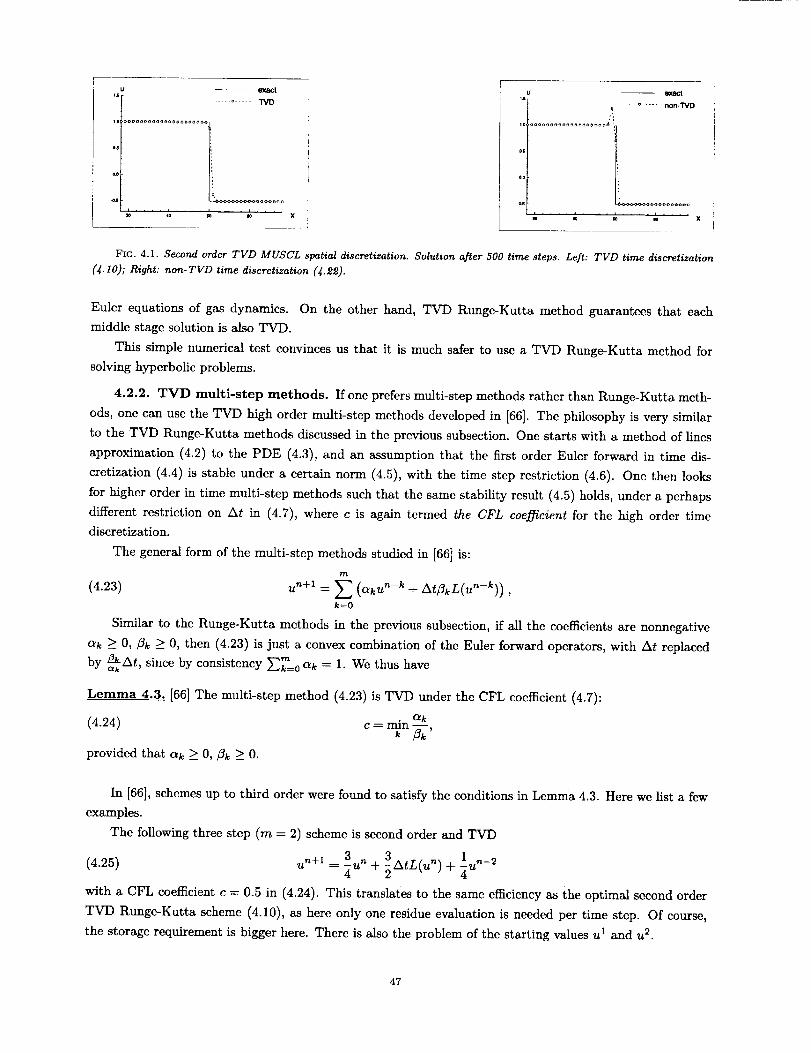
0+0
-- m_c|
..... o--- TVD
_°°°_°°°°°°°°°°°°°°°'qt:o_o_+ooo+o+ocoooo_!
, .... , ....... , , , ,SO 40 so I0
is
:0
0:
0oooooooooooo_ooooo_
.... * ..... non-TVO
• i ....w lo i0 io x
FIG. 4.1. Second order TVD MUSCL spatial discretization. Solution after 500 time steps. Left: TVD time discretization(4.10); Right: non-TVD time discretization (_._).
Euler equations of gas dynamics. On the other hand, TVD Runge-Kutta method guarantees that each
middle stage solution is also TVD.
This simple numerical test convinces us that it is much safer to use a TVD Runge-Kutta method for
solving hyperbolic problems.
4.2.2. TVD multi-step methods. If one prefers multi-step methods rather than Runge-Kutta meth-
ods, one can use the TVD high order multi-step methods developed in [66]. The philosophy is very similar
to the TVD Runge-Kutta methods discussed in the previous subsection. One starts with a method of lines
approximation (4.2) to the PDE (4.3), and an assumption that the first order Euler forward in time dis-
cretization (4.4) is stable under a certain norm (4.5), with the time step restriction (4.6). One then looks
for higher order in time multi-step methods such that the same stability result (4.5) holds, under a perhaps
different restriction on At in (4.7), where c is again termed the CFL coej_cient for the high order timediscretization.
The general form of the multi-step methods studied in [66] is:
(4.23) u n+l = _ (_ku n-k + Atl3kL(un-k)),k=O
Similar to the Runge-Kutta methods in the previous subsection, if all the coefficients are nonnegative
c_k ___0, fl_ > 0, then (4.23) is just a convex combination of the Euler forward operators, with At replaced
by _-_-kAt, since by consistency _'-:k___0C_k = 1. We thus have
Lemma 4.3. [66] The multi-step method (4.23) is TVD under the CFL coefficient (4.7):
. _k
(4.24) c =
provided that _k >_ 0, _k _> 0.
In [66], schemes up to third order were found to satisfy the conditions in Lemma 4.3. Here we list a few
examples.
The following three step (m = 2) scheme is second order and TVD
(4.25) un+Z 3 ,_ _ 1 ___= -_u + AtL(u n) + _u
with a CFL coefficient c = 0.5 in (4.24). This translates to the same efficiency as the optimal second order
TVD Runge-Kutta scheme (4.10), as here only one residue evaluation is needed per time step. Of course,
the storage requirement is bigger here. There is also the problem of the starting values u I and u 2.
47
The following five step (m = 4) scheme is third order and TVD
25 n 25 n 7 ,_-4 5(4.26) un+l = -_u + -_AtL(u ) + -_u + AtL(u n-')
with a CFL coefficient c : 0.5 in (4.24). This translates to a better efficiency than the optimal third order
TVD Runge-Kutta scheme (4.11), as here only one residue evaluation is needed per time step. Of course,
the storage requirement is much bigger here. There is also the problem of the starting values u 1, u 2, u 3 and
U 4 .
There are many other TVD multi-step methods satisfying the conditions in Lemma 4.3 listed in [66]. It
seems that if one uses more storage (larger m) one could get better CFL coefficients.
In [66] we have been unable to find multi-step schemes of order four or higher satisfying the condition
of Lemma 4.3. As in the Runge-Kutta case, we can relax the condition ilk --> 0 by introducing the adjoint
operator L. We thus have
Lemrna 4.4. [66] The multi-step method (4.23) is TV'D under the CFL coefficient (4.7):
_k(4.27) c = man --k tilkl'
provided that ak > 0, and L is replaced by L for negative ilk.
Again, notice that, if we have both positive and negative ilk's, then both L(u n) and L(u n) must be
computed, the cost as well as storage requirement will thus be doubled.
We list here a six step (m = 5), fourth order multi-step method which is TVD with a CFL coefficient
c = 0.245 in (4.24) [66]:
237 nu _+_ = 71_80u" + _-_AtL(u )
81 un_ a 165 n-4 1 n-s_ _AtL(un-S)(4.28) +_-_ + _AtL(u ) + -_u
4.2.3. The Lax-Wendroff procedure. Another way to discretize the time variable is by the Lax-
Wendroff procedure [51]. This is also refcrred to as the Taylor series method for discretizing the ODE (4.2).
We will again use the simple 1D scalar conservation law (4.3) as an example to illustrate the procedure,
however it applies to more general multidimensional systems.
Starting from a Taylor series expansion in time:
• At 2
(4.29) u(x, t + At) = u(x, t) + ut(x, t)At + uu(x, t)_ + ...
The expansion is carried out to the desired order of accuracy in time. For example, a second order in time
would need the three terms written out in (4.29). We then use the PDE (4.3) to replace the time derivatives
by the spatial derivatives:
(4.30)
ut(x, t) : - f (u(x, t) )_ = - f'(u(x, t)) ux(x, t);
utt(x, t) = -(f(u(x, t))tx : -(ft (u(x, t) ut(x, t) )x
= ((f'(_(x, t))2_(x, t))x
= 2f'(u(x, t)) f"(u(x, t) (ux(x,t))2 -}-(f'(u(x, t)))2 uxx(x, t);
48
This little exercise in (4.30) should convince us that it is always possible to write all the time derivatives
as functions of the u(x, t) and its spatial derivatives. But the expression could be terribly complicated,
especially for multidimensional systems.
Once this is done, we substitute (4.30) into (4.29), and then discretize the spatial derivatives of u(x, t)
by whatever methods we use. For example, in the cell averaged (finite volume) ENO schemes discussed
in Sect. 2.3.1, we proceed as follows. We first integrate the PDE (2.65) in space-time over the region
[x,_½,x,+½] x [tn, t n+l] to obtain
(4.31) _n+l = _n _ Ax--'-_i f(u(xi+½, t))dt - f(u(xi_½, t))dt
Then, we use a suitable Gaussian quadrature to discretize the time integration for the flux in (4.31):
1 _tl '*+_(4.32) -_ f(u(xi+ ½, t))dt _ E waf(u(x,+ 3' tn + _aAt),Ct
where 3a and w_ are Gaussian quadrature nodes and weights. Next we replace each
f(u(xi+½, tn + t3aAt)
by a monotone flux:
(4.33) f(u(x,+½,t n + _aAt) _ h (u(x-_+½,t n + _aAt), u(x++½,t n + _At)) ,
and use the Lax-Wendroff procedure (4.29)-(4.30) to convert
u(x, ½,tn + Z zxt)
to u(x_i+ ½, t _) and its spatial derivatives also at t_, which can then be obtained by the reconstructions p(x)
inside Ii and Ii+l. Notice that the accuracy is just enough in this procedure, as each derivative of the
reconstruction p(x) will be one order lower in accuracy, but this is compensated by the At in front of it in
(4.29).
This Lax-Wendroff procedure, comparing with the method of lines approach coupled with TVD Runge-
Kutta or multi-step time discretizations, has the following advantages and disadvantages.
Advantages:
1. This is a truly one step method, hence it is quite compact (a second order method in space and time
uses only three cells on time level n to advance to time level n + I for one cell), and there are no
complications such as boundary conditions needed in middle stages;
2. It utilizes the PDE more extensively than the method of lines approach. This is also one reason that
it can be so compact.
Disadvantages:
1. The algebra is very, very complicated for multi dimensional systems. This also increases operation
counts for complicated nonlinear systems;
2. It is more difficult to prove stability properties (e.g. TVD) for higher order methods in this frame-
work;
3. It is difficult and costly to apply this procedure to the conservative finite difference framework
established in Sections 2.3 and 3.3.
49
4.3. Formulation of the ENO and WENO Schemes for the Hamilton-Jacobi Equations. In
this section we describe high order ENO and W'ENO approximations to the Hamilton-Jacobi equation:
f Ct +H(¢_,¢_) = 0(4.34)
¢(x, y,0) = ¢°(x, y)
where H is a locally Lipschitz continuous Hamiltonian and the initial condition ¢0 (x, y) is locally Lipschitz
continuous. We have written the equation (4.34) in two space dimensions, but the discussion is valid for
other space dimensions as well.
As is well known, solutions to (4.34) are Lipschitz continuous but may have discontinuous derivatives,
regardless of the smoothness of ¢°(x, y). The non-uniqueness of such generalized solutions also necessitates
the definition of viscosity solutions, to single out a unique, practically relevant solution. The viscosity
solution to (4.34) is a locally Lipschitz continuous function ¢(x, y, t), which satisfies the initial condition and
the following property: for any smooth function tb(x, y, t), if (Xo, Y0, to) is a local maximum point of ¢ - ¢,
then
(4.35) ¢_(xo,yo,to) + H(¢x(x0, yo,to) + ¢_(x0,yo,to)) < 0,
and, if (x0, Y0, to) is a local minimum point of ¢ - _b, then
(4.36) ¢_(xo,y0,to) + H(¢_(_0, yo,to) + ¢_(_0, y0,to)) > 0.
Of course, the above definition means that whenever ¢(x, y, t) is differentiable, (4.34) is satisfied in the
classical sense. Viscosity solution dcfined this way exists and is unique. For details and equivalent definitions
of viscosity solutions, see Crandall and Lions [22].
Hamilton-Jacobi equations are actually easier to solve than conservation laws, because the solutions are
typically continuous (only the derivatives are discontinuous).
As before, given mesh sizes Ax, Ay and At, we denote the mesh points as (xi, yj, tn) = (lAx, jAy, nat).
The numerical approximation to the viscosity solution ¢(x_, yj, tn) of (4.34) at the mesh point (x_, yj, tn)
is denoted by ¢_j. We again use a semi-discrete (discrete in the spatial variables only) formulation as a
middle step in designing algorithxns. In such cases, the numerical approximation to the viscosity solution
¢(x_, y3, t) of (4.34) at the mesh point (xi, yj, t) is denoted by ¢ij (t), the temporal variable t is not discretized.
We will also use the notations D_=¢ij = ....+(_'+_A_--¢O)and D:_¢ij = _=(¢"J+_--_'J)A_to denote the first order
forward/backward difference approximations to the left and right derivatives of ¢(x, y) at the location (x,, yj).
Since the viscosity solution to (4.34) is usually only Lipschitz continuous but not everywhere differen-
tiable, the formal order of accuracy of a numerical scheme is again defined as that determined by the local
truncation error in the smooth regions of the solution. Thus, a monotone scheme of the form
(4.37) . = (¢,__,___,...,¢_+_,_+_)
where G is a non-decreasing function of each argument, is called a first order scheme, although the provable
1 [23]. In the semi-discrete formulation, a five point monotoneorder of accuracy in the Lo¢ norm is just
scheme (it does not pay to use more points for a monotone scheme because the order of accuracy of a
monotone scheme is at most one [36]) is of the form
(4.38) d¢ij (t) = -/?/(D_ ¢_j (t), D __¢ij (t), D__ ¢ij (t), D y_¢ij (t)).
5o
ThenumericalHamiltonian// is assumed to be locally Lipschitz continuous, consistent with H: /:/(u, u, v, v) --
H(u, v), and is non-increasing in its first and third arguments and non-decreasing in the other two. Sym-
bolicaUy H(l, T, _, T)- It is easy to see that, if the time derivative in (4.38) is discretized by Euler forward
differencing, the resulting fully discrete scheme, in the form of (4.37), will be monotone when At is suitably
small. We have chosen the semi-discrete formulation (4.38) in order to apply suitable nonlinearly stable high
order Runge-Kutta type time discretization, see Sect. 4.2.
Semi-discrete or fully discrete monotone schemes (4.38) and (4.37) are both convergent towards the
viscosity solution of (4.34) [23]. However, monotone schemes are at most first order accurate. As before, we
will use the monotone schemes as building blocks for higher order ENO and WENO schemes.
ENO schemes were adapted to the Hamilton-Jacobi equations (4.34) by Osher and Sethian [59] and
Osher and Shu [60]. As we know now, the key feature of the ENO algorithm is an adaptive stencil high order
interpolation which tries to avoid shocks or high gradient regions whenever possible. Since the Hamilton-
Jacobi equation (4.34) is closely related to the conservation law (3.21), in fact in one space dimension
they are exactly the same if one takes u -- Cx, it is not surprising that successful numerical schemes for
the conservation laws (3.21), such as ENO and WENO, can be applied to the Hamilton-Jacobi equation
(4.34). ENO and WENO schemes, when applied to Hamilton-iIacobi equations (4.34), can produce high
order accuracy in the smooth regions of the solution, and sharp, non-oscillatory corners (discontinuities in
derivatives).
There are many monotonc Hamiltonians [23], [59], [60]. In this section we mainly discuss the following
tWO:
1. For the special case H(u, v) = f(u 2, v 2) where f is a monotone function of both arguments, such as
the example H(u, v) = _ + v 2, we can use the Oshcr-Sethian monotone Hamiltonian [59]:
(4.39) I:I°S(u+, u-, v+ , v-) = f(u 2, v_)
where, if f is a non-increasing function of u 2, u s is implemented by
(4.40) u 2 = (min(u-, 0)) 2 + (max(u +, 0)) 5
and, if f is a non-decreasing function of u 2, u 2 is implemented by
(4.41) u 2 = (min(u +, 0)) 2 + (max(u-, 0)) 2
Similarly for v 2. This Hamiltonian is purely upwind (i.e. when H(u, v) is monotone in u in the
relevant domain [u-, u +] x Iv-, v+], only u- or u + is used in the numerical Hamiltonian according
to the wind direction), and simple to program. Whenever applicable it should be used. This flux is
similar to the Engquist-Osher monotone flux (2.71) for the conservation laws.
2. For the general H we can always use the Godunov type Hamiltonian [5], [601:
(4.42) -fI°(u +, u-, v +, v-) -- ext_e_(,,-,_+) ext_er(v-,_+) H(u, v)
where the extrema are defined by
{ min_<_<b if a _< b(4.43) eXtuEl(a'b) = maxb<u< a if a > b
Codunov Hamiltonian is obtained by attempting to solve the Riemann problem of the equation
(4.34) exactly with piecewise linear initial condition determined by u=k and v _:. It is in general not
51
unique, because in general minu max, H(u, v) _ maxv minu H(u, v) and interchanging the order of
the two ext's in (4.42) can produce a different monotone Hamiltonian.
Godunov Hamiltonian is purely upwind and is the least dissipative among all monotone Hamiltonians
[57]. However, it might be extremely difficult to program, since in general analytical expressions for
things like min,, maxv Hiu , v) can be quite complicated. The readers will be convinced by doing the
exercise of obtaining the analytical expression and programming H G for the ellipse in ellipse case in
image processing where H(u, v) = x/au 2 + 2buy + cv 2. For this case the Osher-Sethian Hamiltonian
H °s does not apply.
We are now ready to discuss about higher order ENO or WENO schemes for i4.34). The framework is
quite simple: we simply replace the first order scheme (4.38) by:
d(4.44) _¢,j (t) = -/?/(u + (t), u_ it), v + it), v_ (t))
where u_it ) are high order approximations to the left and right x-derivatives of ¢(x, y, t) at ix,, yj, t):
(4.45) u_(t) = 0¢, +_-_tx,, yj, t) + O(Ax r)
Similarly for v_ (t). Notice that there is no cell-averaged version now.
The key feature of ENO to avoid numerical oscillations is through the following interpolation procedure
to obtain u_it ) and v_(t). These are just the same ENO procedure we discussed before in Sect. 2.2. We
repeat it here with its own notations:
ENO Interpolation Algorithm: Given point values f(x¢), j = 0, +1, +2,..- of a (usually piecewise
smooth) function f(x) at discrete nodes xj, we associate an r-th degree polynomial P_/2(x) with each
interval [xj, Xj+l], with the left-most point in the stencil as xk_:l , constructed inductively as follows:
(1) P/411/2(x) = f[xj] + f[xj,xj+l]i x xj), (1)- k,.i. = j;(l -- 1) f,l -- 1
(2) If kin, . and P[i+w2(x) are both defined, then let
a (l) ._ f[Xk_;_),'", Xk_;_}+l]
b(l) --- f[xk_::)-l''' '' Xk_::) +l-l]
and
(0 = k(t-_) q) bq-_)(i) If [aq) t > {b_[, then c (l) = b(0 and kmi n -ml, --1; otherwise c q) = a(0 and kmi n = "'mi, ;
(ii) PJ'+ll/2(x ) = pLl-1, , c(t) ,'-,k_:_)+l-1,3+1/_(X) + lii=k(_._) (x- xi) •
In the above procedure f[.,..-, .] are the standard Newton dividcd differences, inductively defined as
f[xl,x2,... ,xk+l] = I[_2,---,_+_]-f[_,.-.,z_] with ][xl] = f(xl).
ENO Interpolation Algorithm starts with a first degree polynomial Pj!+ll/2(x) interpolating the function
f(x) at the two grid points xj and xj+l. If we stop here, we would obtain the first order monotone scheme.
When higher order is desired, we will in each step add just one point to the existing stencil, chosen from
the two immediate neighbors by the size of the two relevant divided differences, which measures the local
smoothness of the function f(x).
The approximations to the left and right x-derivatives of ¢ are then taken as
(4.46) u_ = _x P_/2d(xi)"
: 52
whereP_I/2j (x) is obtained by the ENO Interpolation Algorithm in the x-direction, with y = yj and t both
fixed, v_ are obtained in a similar fashion. The resulting ODE (4.44) is then discretized by an r-th order
TVD Runge-Kutta time discretization in Sect. 4.2 to guarantee nonlinear stability. More specifically, the
high order Runge-Kutta method we use in Sect. 4.2 will maintain TVD (total-variation-diminishing) or other
stability properties, if these properties are valid for the simple first order Euler forward time discretization
of the ODE (4.44). Notice that this is different from the usual linear stability requirement for the ODE
solver. We thus obtain both nonlinear stability and high order accuracy in time. The second order (r -- 2)
and third order (r = 3) methods we use which has this stability property are given by (4.10) and (4.11),
respectively.
Time step restriction is taken as
(4.47) At _xx max_,,v U(u,v) + max H(u, v) _< 0.6
where the maximum is taken over the relevant ranges of u, v. Here 0.6 is just a convenient number used in
practice. This number should be chosen between 0.5 and 0.7 according to our numerical experience.
WENO schemes can be used in a similar fashion for Hamilton-Jacobi equations [45]. We will not presentthe details here.
5. Applications.
5.1. Applications to Compressible Gas Dynamics. One of the main application areas of ENO
and WENO schemes is compressible gas dynamics.
In 3D, Euler equations of gas dynamics are written as
+ f(u)x + 9(u) + h(Uh = o
where
U = (p, pu, pv, pw, E),
f(U) = (pu, pu 2 + P, puv, puw, u(E + P)),
g(U) = (pv, puv, pv 2 + P, pvw, v(E + P)),
h(U) = (pw, puw, pvw, pw 2 + P, w(E + P)).
Here p is density, (u, v, w) is the velocity, E is the total energy, P is the pressure, related to the total energy
E by
E- P 1 2 v 2-1 + p(u + +w 2)
with 7 = 1.4 for air.
For the form of Navier-Stokes equations, for the eigenvalues and eigenvectors needed for the characteristic-
wise ENO and WENO schemes, and for those equations appearing in curvilinear coordinates, see, e.g. [71].
We mention the following applications of ENO and WENO schemes for compressible flow calculations:
53
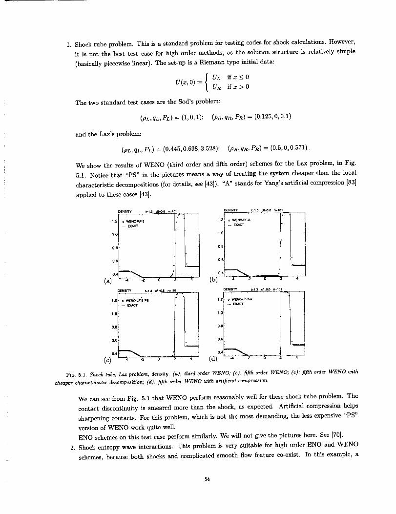
1. Shocktubeproblem.Thisisa standardproblemfortestingcodesforshockcalculations.However,it is not thebesttest casefor highordermethods,asthe solutionstructureis relativelysimple(basicallypiecewiselinear).Theset-upisaRiemanntypeinitial data:
( UL ifx<0U(x, 0) )
UR if z > 0
The two standard test cases are the Sod's problem:
(PL, qL,PL) = (1,0,1); (PR, qR, PR) = (0.125,0,0.1)
and the Lax's problem:
(PL, qL, PL) = (0.445, 0.698, 3.528); (PR, qa, PR) = (0.5, 0, 0.571).
We show the results of WENO (third order and fifth order) schemes for the Lax problem, in Fig.
5.1. Notice that "PS" in the pictures means a way of treating the system cheaper than the local
characteristic decompositions (for details, see [43]). "A" stands for Yang's artificial compression [83]
applied to these cases [43].
1.2
1.0
0.8
0.6
0.4
(a)
0.8
0.6
0.4'
(c)
:)e'NS_ . _!.¢ _-0.6 ,=,O,r_ , !o , • /
o WENO-RF-34
--EXACT°
J ., I0 2 4
1.2 o WENO-LF-'5-1=S
-- EXACT
1.0
_-2
[_NS [TY , t_1.3 Cfl=_.8 fl--'0] _.=
DENSITY t=1.3 cfl=0.8 n=101
1.2_ o WENO-RF-5
-- EXACT .
1.0_
0.8
0.6
(b) _ "_ 0 2 ' 4
DENSITY t=1.3 eft=0.6 n=101
1.2[ o W',_IO-LF-5-A--EXACT
1.0[
0.8[
O.6F
(d) -4 -2 o
4
J4
I
I
2 4
FIG. 5.1. Shock tube, Lax problem, density. {a): third order WENO; (b): fifth order WENO; (c): fifth order WENO with
cheaper characteristic decomposition; (d): fifth order WENO with artificial compression.
.
We can see from Fig. 5.1 that WENO perform reasonably well for these shock tube problem. The
contact discontinuity is smeared more than the shock, as expected. Artificial compression helps
sharpening contacts. For this problem, which is not the most demanding, the less expensive "PS"
version of WENO work quite well.
ENO schemes on this test case perform similarly. We will not give the pictures here. See [70].
Shock entropy wave interactions. This problem is very suitable for high order ENO and WENO
schemes, because both shocks and complicated smooth flow feature co-exist. In this example, a
54
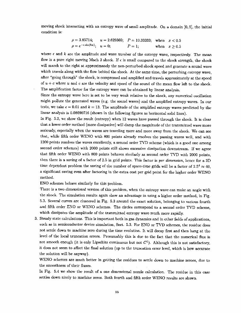
moving shock interacting with an entropy wave of small amplitude. On a domain [0, 5], the initial
condition is:
p = 3.85714; u--- 2.629369; P = 10.33333; when x < 0.5
p = e-eSin(kx); U = 0; P = 1; when x > 0.5
where e and k are the amplitude and wave number of the entropy wave, respectively. The mean
flow is a pure right moving Mach 3 shock. If e is small compared to the shock strength, the shock
will march to the right at approximately the non-perturbed shock speed and generate a sound wave
which travels along with the flow behind the shock. At the same time, the perturbing entropy wave,
after "going through" the shock, is compressed and amplified and travels approximately at the speed
of u + c where u and e are the velocity and speed of the sound of the mean flow left to the shock.
The amplification factor for the entropy wave can be obtained by linear analysis.
Since the entropy wave here is set to be very weak relative to the shock, any numerical oscillation
might pollute the generated waves (e.g. the sound waves) and the amplified entropy waves. In our
tests, we take • = 0.01 and k = 13. The amplitude of the amplified entropy waves predicted by the
linear analysis is 0.08690716 (shown in the following figures as horizontal solid lines).
In Fig. 5.2, wc show the result (entropy) when 12 waves have passed through the shock. It is clear
that a lower order method (more dissipative) will damp the magnitude of the transmitted wave more
seriously, especially when the waves are traveling more and more away from the shock. We can see
that, while fifth order WENO with 800 points already resolves the passing waves well, and with
1200 points resolves the waves excellently, a second order TVD scheme (which is a good one among
second order schemes) with 2000 points still shows excessive dissipation downstream. If wc agree
that fifth order WENO with 800 points behaves similarly as second order TVD with 2000 points,
then there is a saving of a factor of 2.5 in grid points. This factor is per dimension, hence for a 3D
time dependent problem the saving of the numbcr of space-time grids will be a factor of 2.54 _ 40,
a significant saving even after factoring in the extra cost per grid point for the higher order WENO
method.
ENO schemes behave similarly for this problem.
There is a two dimensional version of this problem, when the entropy wave can make an angle with
the shock. The simulation results again show an advantage in using a higher order method, in Fig.
5.3. Several curves are clustered in Fig. 5.3 around the exact solution, belonging to various fourth
and fifth order ENO or WENO schemes. The circles correspond to a second order TVD scheme,
which dissipates the amplitude of the transmitted entropy wave much more rapidly.
3. Steady state calculations. This is important both in gas dynamics and in other fields of applications,
such as in semiconductor device simulation, Sect. 5.3. For ENO or TVD schemes, the residue does
not settle down to machine zero during the time evolution. It will decay first and then hang at the
level of the local truncation errors. Presumably this is due to the fact that the numerical flux is
not smooth enough (it is only Lipschitz continuous but not C1). Although this is not satisfactory,
it does not seem to affect the final solution (up to the truncation error level, which is how accurate
the solution will be anyway).
WENO schemes are much better in getting the residues to settle down to machine zeroes, due to
the smoothness of their fluxes.
In Fig. 5.4 we show the result of a one dimensional nozzle calculation. The residue in this case
settles down nicely to machine zeros. Both fourth and fifth order WENO results are shown.
55
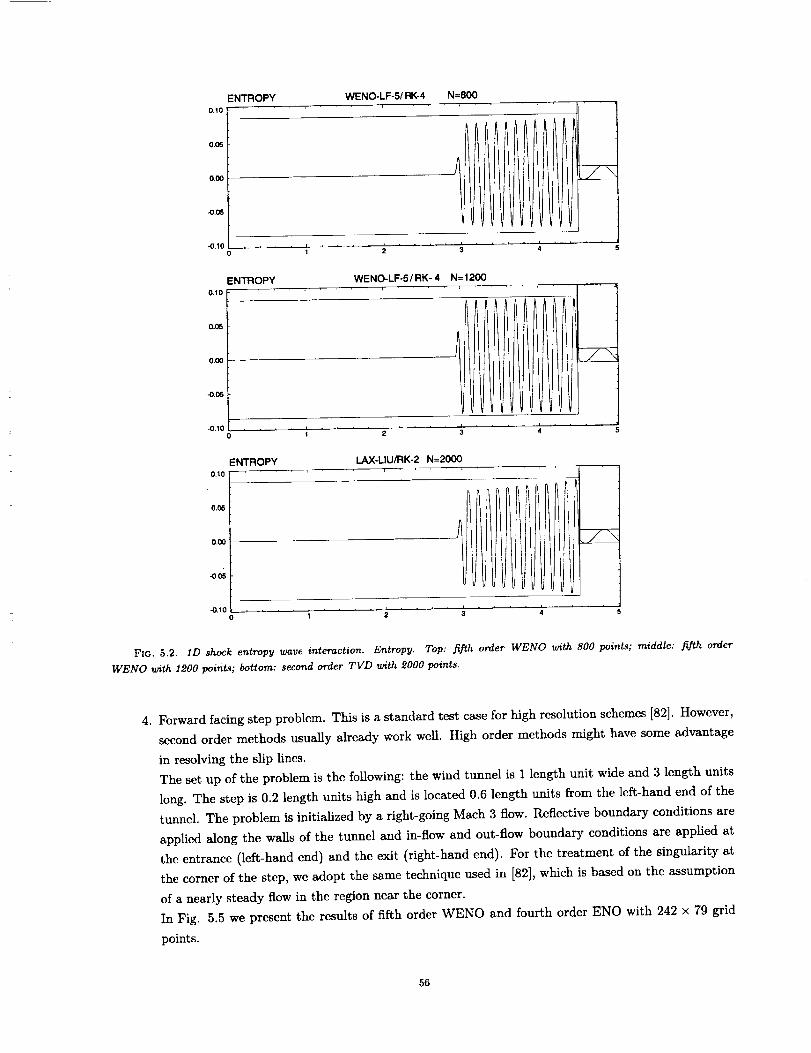
0.10
0.06
0,00
.0,05
ENTROPY WENO-LF-5/RK-4 N=800
0.10
0.05
0.00
-0.06
ENTROPY WENO-LF-5/RK- 4 N=1200r T 1
i
-0.10
0 I 2 3 4
0.10
0.05
ENTROPY LAX-LIU/RK-2 N=2000
0 I 2 3
Fzc. 5.2. ID shock entropy wave interaction. Entropy. Top: fifth order WENO with 800 points; middle: fifth order
WENO with 1_00 points; bottom: second order TVD with _000 points.
4, Forward facing step problem. This is a standard test case for high resolution schemes [82]. However,
second order methods usually already work well. High order methods might have some advantage
in resolving the slip lines.
The set up of the problem is the following: the wind tunnel is 1 length unit wide and 3 length units
long. The step is 0.2 length units high and is located 0.6 length units from the left-hand end of the
tunnel. The problem is initialized by a right-going Mach 3 flow. Reflective boundary conditions are
applied along the walls of the tunnel and in-flow and out-flow boundary conditions are applied at
the entrance (left-hand end) and the exit (right-hand end). For the treatment of the singularity at
the corner of the step, wc adopt the same technique used in [82], which is based on the assumption
of a nearly steady flow in the region near the corner.
In Fig. 5.5 we present the results of fifth order WENO and fourth order ENO with 242 × 79 grid
points.
56
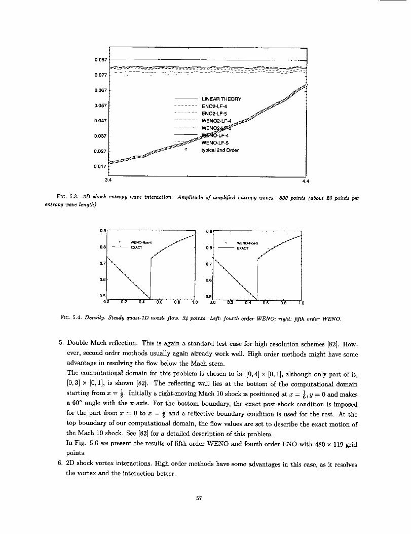
0.087
0.077
0.067
0.057
0.047
0.037
0.027
0.017 -
3.4
-- LINEAR THEORY
[ ....... ENo -LF .............ENO2-LF-5...... WENO2-LF_
................ W_
WENO-LF-5
o typical 2nd Order
4.4
Fzc. 5.3. $D shock entropy wave interaction. Amplitude of amplified entropy waves. 800 points (about PO points per
entropy wave length).
[I " WENO.-Roe_4
0.6
0.5 ....0.0 0.2 0.4 0.6 0.8 1.0
0.gr • , , , , -
i o WENO-Roe-5
O.S
11.5
0.0 0.2 0.4 0.6 0.8 1.0
FIG. 5.4. Density. Steady quasi-lD nozzle flow. 3,_ points. Left: fourth order WENO; right: fifth order WENO.
5. Double Mach reflection. This is again a standard test case for high resolution schemes [82]. How-
ever, second order methods usually again already work well. High order methods might have some
advantage in resolving the flow below the Mach stem.
The computational domain for this problem is chosen to be [0, 4] × [0, 1], although only part of it,
[0, 3] × [0, 1], is shown [82]. The reflecting wall lies at the bottom of the computational domain
starting from x = 1. Initially a right-moving Mach 10 shock is positioned at x = I, Y = 0 and makes
a 60 ° angle with the x-axis. For the bottom boundary, the exact post-shock condition is imposed
for the part from x = 0 to x = _ and a reflective boundary condition is used for the rest. At the
top boundary of our computational domain, the flow values are set to describe the exact motion of
the Mach 10 shock. See [82] for a detailed description of this problem.
In Fig. 5.6 we present the results of fifth order WENO and fourth order ENO with 480 × 119 grid
points.
6. 2D shock vortex interactions. High order methods have some advantages in this case, as it resolves
the vortex and the interaction better.
57
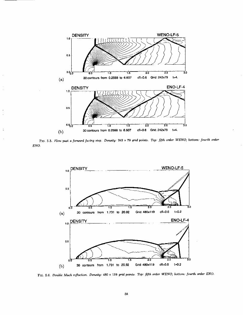
(a)
1,0
0,5
0.%'.0
DENSITY
/
0.5 i .0 1.5
30 contours from 0.2568 to 6.807
WENO-LF-5
" 2'.o .... 2'.s " ' 3.0
cfl=0.6 Grid: 242x79 t--4.
1.0
0,5
O.Oo,.o
(b)
DENSITY ENO-LF-4
0.5 1.0 1.5 2.0 2.5 3.0
30 contours from 0.2568 to 6.607 cfl=0,6 Grid: 242x79 t=4.
FIG. 5.5. Flow past a for'ward facing step. Density: 242 x 79 grid points. Top: fifth order WENO; bottom: fourth order
ENO.
1.0
0.5
(a)
0,0
)ENSITY WENO-LF-5
0.5 1.0 1.5 2.0 2.5 ;_.0
30 contours from 1.731 to 20.92 Grid: 480xl 19 cfl=0,6 t--0.2
(b)
1,0
0.5
)ENSITY ENO-LF-4
0.0 0.5 1.0 1.5 2.0 2.5 3.0
30 contours from 1.731 to 20.92 Grid:480x119 cfl=0.6 t=0.2
Fzc. 5.6. Double Mach reflection. Density: 480 x 119 grid points. Top: fifth order WENO; bottom: fourth order ENO.
58
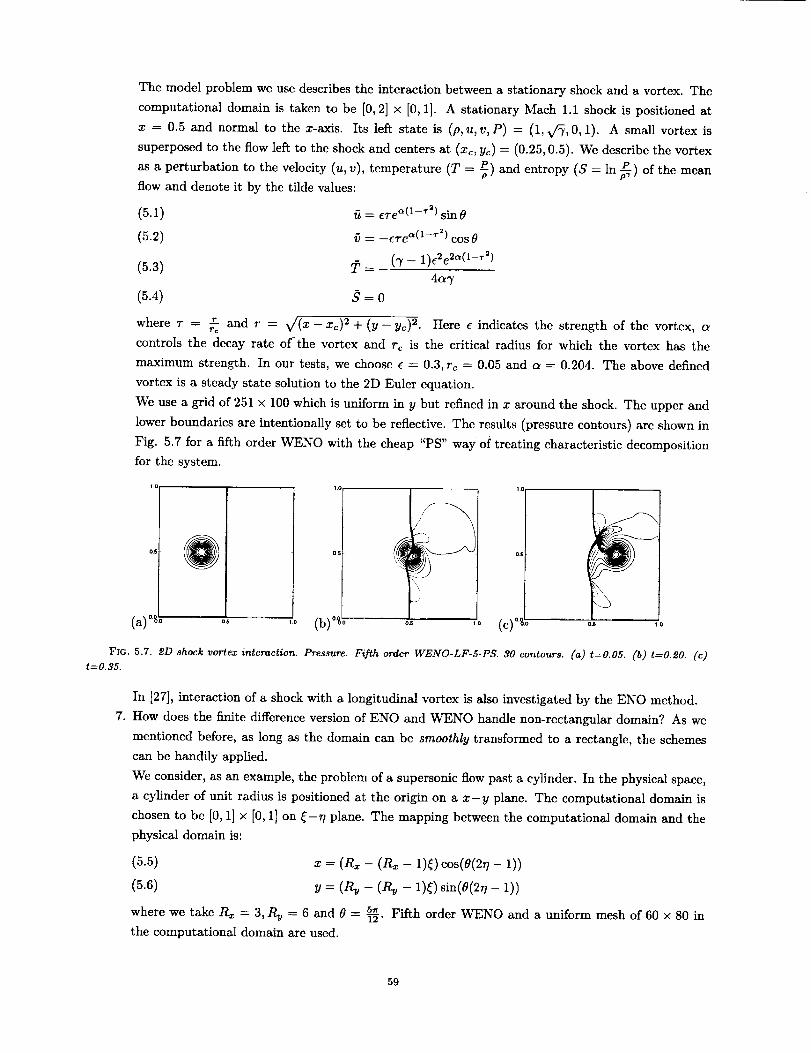
The model problem we use describes the interaction between a stationary shock and a vortex. The
computational domain is taken to be [0, 2] x [0, 1]. A stationary Mach 1.1 shock is positioned at
x -- 0.5 and normal to the x-axis. Its left state is (p, u, v, P) = (1, yr_, 0, 1). A small vortex is
superposed to the flow left to the shock and centers at (xc, Ye) = (0.25, 0.5). We describe the vortex
as a perturbation to the velocity (u, v), temperature (T = P) and entropy (S = In _) of the meanflow and denote it by the tilde values:
(5.1) fi = e're _(1-_2) sin #
(5.2) _ = -eve _(1-_2) cos t_
(5.3) _ = _ (7 - 1)c 2e2_(t-_2)4c_7
(5.4) S = 0
--_ and r = v/(x - xe) 2 + (y - yc)2. Here e indicates the strength of the vortex, awhere 7- -- ro
controls the decay rate of the vortex and re is the critical radius for which the vortex has the
maximum strength. In our tests, we choose e = 0.3, re -- 0.05 and a = 0.204. The above defined
vortex is a steady state solution to the 2D Euler equation.
We use a grid of 251 × 100 which is uniform in y but refined in x around the shock. The upper and
lower boundaries are intentionally set to be reflective. The results (pressure contours) arc shown in
Fig. 5.7 for a fifth order WENO with the cheap "PS" way of treating characteristic decomposition
for the system.
05
(a)°_ ..... (b)°.t] (c)O.%O_S , .0
FIC. 5.7. PD shock vortex interaction. Pressure. Fifth order WENO-LF-5-PS. 30 contours. (a) t=O.05. (b) t--0.20. (c)t=0.35.
7.
In [27], interaction of a shock with a longitudinal vortex is also investigated by the ENO method.
How does the finite difference version of ENO and WENO handle non-rectangular domain? As we
mentioned before, as long as the domain can be smoothly transformed to a rectangle, the schemes
can be handily applied.
We consider, as an example, the problem of a supersonic flow past a cylinder. In the physical space,
a cylinder of unit radius is positioned at the origin on a x-y plane. The computational domain is
chosen to be [0, 1] × [0, 1] on _-_7 plane. The mapping between the computational domain and the
physical domain is:
(5.5) x = (R_ - (R_ - 1)_)cos(O(2_ - 1))
(5.6) y = (P_ - (P_ - 1)_)sin(o(2_- 1))
where we take R, = 3, tlv = 6 and _ = 5_ Fifth order WENO and a uniform mesh of 60 × 80 in
the computational domain are used.
59
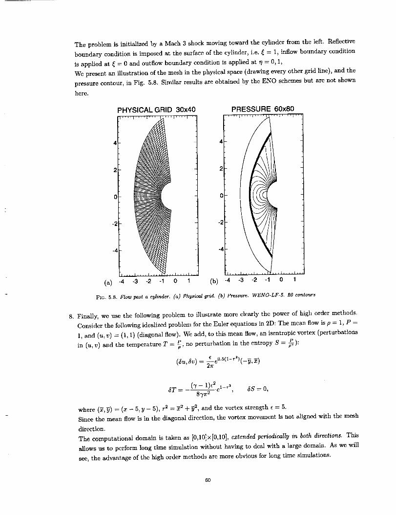
Theproblemis initializedbya Mach3 shockmovingtowardthecylinderfromtheleft.Reflectiveboundaryconditionis imposedat thesurfaceof thecylinder,i.e._= 1, inflow boundary condition
is applied at _ -- 0 and outflow boundary condition is applied at _/-- 0, 1,
We present an illustration of the mesh in the physical space (drawing every other grid line), and the
pressure contour, in Fig. 5.8. Similar results are obtained by the ENO schemes but are not shown
here.
PHYSICAL GRID 30x40 PRESSURE 60x80
4 4
2 2
(] 0
(a) -4 -3 -2 -_ 0 1 (b) -4 -3 -2 -1 0 1
FIC. 5.8. Flow past a cylinder. (a) Physical grid. (b) Pressure. WENO-LF-5. 20 contours
8. Finally, we use the following problem to illustrate more clearly the power of high order mcthods.
Consider the following idealized problem for the Euler equations in 2D: The mean flow is p --- 1, P =
1, and (u, v) = (1, 1) (diagonal flow). We add, to this mean flow, an isentropic vortex (perturbations
in (u, v) and the temperature T ---- -,P no perturbation in the entropy S -- _-_).P 'p
(_u, _v) = _e °'5(1-'b (-_, _)
3T = (9'- 1) C2 1 r 2e - , 5S = O,87r 2
where (5, y) ----(x - 5, y - 5), r 2 = _2 + _2, and the vortex strength e = 5.
Since the mean flow is in the diagonal direction, the vortex movement is not aligned with the mesh
direction.
The computational domain is taken as [0,10]×[0,10], extended periodically in both directions. This
allows us to perform long time simulation without having to deal with a large domain. As we will
see, the advantage of the high order methods are more obvious for long time simulations.
6O
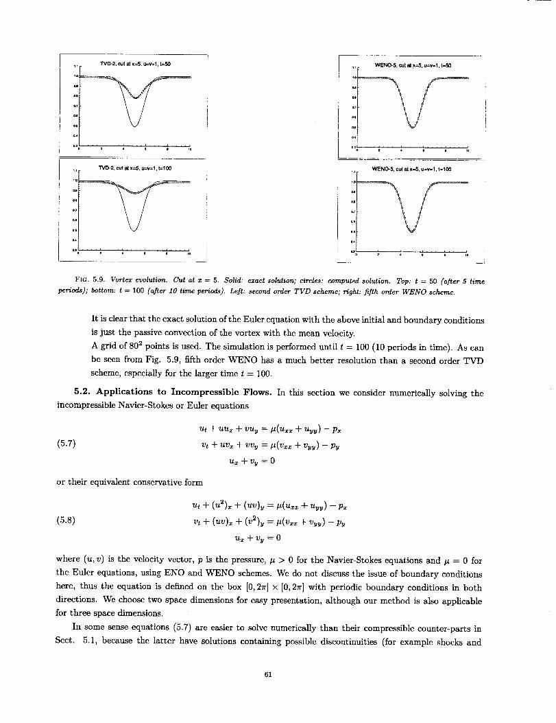
. TVD-2, cut at x=5, u=v=l, t=50
al
........ , , , . . , .....
TVD-2, cut at x=5, u=v=l, t=100
07
O.I
U
OA
]
,. , . , .... ,i = e | vo
WENO-5, cut at x=5, u=v=l, t=100
o.?
al
o.s
a4
. _ , , ju _ _ e i 1o
FIG. 5.9. Vortex evolution. Cut at z = 5. Solid: exact solution; circles: computed solution. Top: t = 50 (after 5 timeperiods); bottom: t = 100 (after 10 time periods}. Left: second order TVD scheme; right: fifth order WENO scheme.
It is clear that the exact solution of the Euler equation with thc above initial and boundary conditions
is just the passive convection of the vortex with the mean velocity.
A grid of 802 points is used. The simulation is performed until t = 100 (10 pcriods in time). As can
be seen from Fig. 5.9, fifth order WENO has a much better resolution than a second order TVD
scheme, especially for thc larger time t = 100.
5.2. Applications to Incompressible Flows. In this section we consider numerically solving the
incompressible Navier-Stokes or Euler equations
(5.7)ut + uux + vuy = #(ux= + uvv ) - p=
vt + uv= + vvv = #(v== + vuu ) - py
Ux -F Vv = 0
or their equivalent conservative form
(5.8) v, + ( v)x + = + -
IZ x q- Vy = 0
where (u, v) is the velocity vector, p is the pressure, /_ > 0 for the Navier-Stokes equations and/z = 0 for
the Euler equations, using ENO and WENO schemes. We do not discuss the issue of boundary conditions
here, thus the equation is defined on the box [0, 2r] × [0, 27r] with periodic boundary conditions in both
directions. We choose two space dimensions for easy presentation, although our method is also applicable
for three space dimensions.
In some sense equations (5.7) are easier to solve numerically than their compressible counter-parts in
Sect. 5.1, because the latter have solutions containing possible discontinuities (for example shocks and
61
contact discontinuities). However, the solution to (5.7), even if for most cases smooth mathematically, may
evolve rather rapidly with time t and may easily become too complicated to be fully resolved on a feasible
grid. Traditional linearly stable schemes, such as spectral methods and high-order central difference methods,
are suitable for the cases where the solution can be fully resolved, but typically produce signs of instability
such as oscillations when small scale features of the flow, such as shears and roll-ups, cannot be adequately
resolved on the computational grid. Although in principle one can always overcome this difficulty by refining
the grid, today's computer capacity seriously restricts the largest possible grid size.
As we know, the high resolution "shock capturing" schemes such as ENO and WENO are based on the
philosophy of giving up fully resolving rapid transition regions or shocks, just to "capture" them in a stable
and somehow globally correct fashion (e.g., with correct shock speed), but at the same time to require a
high resolution for the smooth part of the solution. The success of such an approach for the conservation
laws is documented by many examples in these lecture notes and the references. One example is the one
and two dimensional shock interaction with vorticity or entropy waves [70], [71]. The shock is captured
sharply and certain key quantities related to the interaction between the shock and the smooth part of the
flow, such as the amplification and generation factors when a wave passes through a shock, are well resolved.
Another example is the homogeneous turbulence for compressible Navier-Stokes equations studied in [71].
In one of the test cases, the spectral method can resolve all the scales using a 2562 grid, while third order
ENO with just 642 points can adequately resolve certain interesting quantities although it cannot resolve
local quantities achieved inside the rapid transition region such as the minimum divergence. The conclusion
seems to be that, when fully resolving the flow is either impossible or too costly, a "capturing" scheme such
as ENO can be used on a coarse grid to obtain at least some partial information about the flow.
We thus expect that, also for the incompressible flow, we can use high-order ENO or WENO schemes
on a coarse grid, without fully resolving the flow, but still get back some useful information.
A pioneer work in applying shock capturing compressible flow techniques to incompressible flow is by
Bell, Colella and Glaz [6], in which they considered a second order Godunov type discretization, investigated
the projection into divergence-free velocity fields for general boundary conditions, and discussed accuracy of
time discretizations. Higher order ENO and WENO schemes for incompressible flows are extensions of such
methods.
We solve (5.8) in its equivalent projection form
(5.9) ()u __p _ _ v 2 +# +V t UV V "Ox y xx yy
where P is the H°dge pr°jecti°n int° divergence-free ficlds' i'e" if ( ft ) = P ( U ) ' then ftx + _y = O and_v
_3u - fix = vy - ux. See, e.g., [6]. For the current periodic case the additional condition to obtain a unique
projection P is that the mean values of u and v are preserved, i.e., f:" ]:_ ft(x, y)dxdy = f:_r f:, u(x, y)dxdy
and y) xd :We use Nx and N u (even numbers) equally spaced grid points in x and y, respectively. The grid sizes
are denoted by Ax = _ and Ay = N___,,and the grid points are denoted by xi = lAx and yj = jAy. The
approximated numerical values of u and v at the grid point (x_, yj) are denoted by u0 and vii.
We first describe the numerical implementation of the projection P. In the periodic case this is easily
62
achieved in the Fourier space. We first expand u and v using Fourier collocation:
(5.10) uN(x,y)= vN(x.y)=Z: Z:
where I = V/S] -, ftkz and _3kl are the Fourier collocation coefficients which can be computed from the point
values uij and v_j, using either FFT or matrix-vector multiplications. The detail can be found in, e.g., [9].
Derivatives, either by spectral method or by central differences, involve only multiplications by factors d_ or
d_t in (5.10) because e z(k_+ty) are eigenfunctions of such derivative operators. For example,
(5.11)
forspectralderivatives;
(5.12)
d_ = Ik, _ -- I1
21sin(_) 21sin(_)d_- Ax ' d_t= Ay
for the second order central differences which, when used twice, will produce the second order central
difference approximation _,,.,-2w,+w,_, for w_, andAx_
d_ = 2Iv/(1 - cos(kAx))(7 - eos(kAx))Ax
(5.13) _ = 2iv/(1 - cos(lAy))(7- eos(l_y))Ay
for the fourth order central differences which, when used twice, will produce the fourth order central difference
approximation 1s(_°'*_+_'-Q-(_'#2+_-_)-3°_'12A_ for w_. High order filters, such as the exponential filter [55],
[46]:
_a(A- )21'(5.14) a_ = e-_(_ )_, af = e -"_-
where 2p is the order of the filter and a is chosen so that e -_ is machine zero, can be used to enhance thc
stability while keeping at least 2p-th order of accuracy. This is especially helpful when the projection P is
used for the under-resolved coarse grid with ENO methods. We use the fourth order projection (5.13) and
the filter (5.14) with 2p = 8 in our calculations. This will guarantee third order accuracy (fourth order in
L1) of the ENO scheme. We will denote this combination (the fourth order projection plus the eighth order
()filtering) by P4. To be precise, if u = P4 and ukl and Vkt are Fourier collocation coefficients of_? v
u and v, then the Fourier collocation coefficients of ti and 0 are given by
z ud_t (dUttfi - d_9) -d_(d_t f_ - d_9)(5.15) u=aka , (_k)2-_(_-(_-----_, v=a_a_ (d_)2 +-(-d_l--_
where a z and cr_ are defined by (5.14) with 2p -- 8, and d_ and d_t are defined by (5.13).
Next we shall describe the ENO scheme for (5.8). Since (5.8) is equivalent to the non-conservative form
(5.7), it is natural to implement upwinding by the signs of u and v, and to implement ENO equation by
equation (the component version described in Sect. 2.3.5). The r-th order ENO approximation of, e.g., (u2),
is thus carried out using the ENO Procedure 4.2. We mention a couple of facts needing attention:
1. Take f(x) = u2(x, y) with y fixed. We start with the point values fi = f(x,);
63
(5.17)
obtaining:
2. The stencil of the reconstruction is determined adaptively by upwinding and smoothness of f(x). It
starts with either xj or xj+l according to whether u > 0 or u < 0.
There are two ways to handle the second derivative terms for the Navier-Stokes equations. One can
absorb them into the convection part and treat them using ENO. For example, f(x) = u2(x, y) can be
replaced by f(x) = u2(x, y) - .u(x, y)_, where u(x, y)_ itself can be obtained using either ENO or central
difference of a suitable order. The remaining procedure for computing f(x)x would be the same as described
above. Another simpler possibility is just to use standard central differences (of suitable order) to compute
the double derivative terms. Our experience with compressible flow is that there is little difference between
the two approaches, especially when the viscosity # is small.
In the above we have described the discretization for the spatial derivatives
[(-) (-)(5.16) L O _ - - +. +UV Y 2 V V X = X i
x y $x, yy
Y=Yj
We then use the third order TVD (total variation diminishing) Runge-Kutta method (4.11) to discretize the
resulting ODE:
(U)=p.LOV ¢
(5.18)
(:)("
n+l
V
[(.)n= P4 + AtL13
u I u 1Ate,)=P4 + _ +
v v 4 J
=P4 +_ -J-gA jjV V
Notice that we have used the property P4 o P4 =/)4 in obtaining the discretization (5.18) from (5.17).
This explicit time discretization is expected to be nonlinearly stable under the CFL condition
(5.19) At ax i I+ +2. _+ <1t i,j
For small. (which is the case we are interested in) this is not a serious restriction on At.
We present some numerical examples in the following.
Example 5.1: This example is used to check the third order accuracy of our ENO scheme for smooth
solutions. We first take the initial condition as
(5.20) u(x, y, O) = - cos(x) sin(y), v(x, y, O) = sin(z) cos(y)
which was used in [6]. The exact solution for this case is known:
(5.21) u(x, y, 0 = - cos(z) sin(y)e-_"*, v(x, y, t) = sin(z) cos(y)_-_"_
We take Ax =Ay = 1 with N = 32, 64,128 and 256. The solution is computed up to t = 2 and the L2
error and numerical order of accuracy are listed in Table 5.1. For the. -- 0.05 case, we list results both
64

TABLE 5.1
Accuracy of ENO Schemes for (12.2).
N #=0
L2 error order
32 9.10(-4)
64 5.73(-5) 3.99
128 3.62(-6) 3.98
256 2.28(-7) 3.99
-- 0.05, central
L2 error ?rder
5.28(-4)3.2o(-5)1.93(-6)
1.18(-7)
±
# = 0.05, ENO
L2 error_ order
4.87(-4) _4.04
4.05
4.03 1.16(-7)
3.09(-5) 3.98
1.89(-6) 4.03
4.03
N
32
64
128
256
L2 diff
1.14(-1)
1.40(-2)
1.46(-3)
1.11(-4)
g=0
order
3.02
3.26
3.77
/_ ----0.05, central
error L2 diff order error
3.20(-2)
1.96(-3) 2.78(-3) 3.52 2.66(-4)
1.69(-4) 1.81(-4) 3.94 1.26(-5)
8.78(-6) 1.09(-5) 4.06 6.91(-7)
# -- 0.05, ENO
L2 diff order t error
.....2.93(-3) 3.62 2.60(-4)
1.80(-4) 4.02 1.18(-5)
1.10(-5) 4.04 7.15(-7)
with fourth order central approximation to the double derivative terms (central) and with ENO to handle
the double derivative terms by absorbing them into the convection part (ENO). We can clearly observe fully
third order accuracy (actually better in many cases because the spatial ENO is fourth order in the L1 sense)
in this table.
Example 5.2: This is our test example to study resolution of ENO schemes when the grid is coarse. It
is a double shear layer taken from [6]:
(5.22) u(x, y, O) = _ tanh((y - 7r/2)/p) y < 7r v(x, y, O) = 5 sin(x)( tanh((37r/2- y)/p) y > 7r
where we take p -- _r/15 and 5 - 0.05. The Euler equations (# = 0) are used for this example. The solution
quickly develops into roll-ups with smaller and smaller scales, so on any fixed grid the full resolution is lost
eventually. For example, the expensive run we performed using 5122 points for the spectral collocation code
(with a 18-th order filter (5.14)) is able to resolve the solution fully up to t = 8, Fig. 5.10, top left, as
verified by the spectrum of the solution (not shown here), but begins to lose resolution as indicated by the
wriggles in the vorticity contour at t -- 10 (not shown here). On the other hand, the ENO runs with 642
and 1282 points produces smooth, stable results Fig. 5.10, top right and bottom left. In Fig. 5.10, bottom
right, we show a cut at x -- r for v at t -- 8. This gives a better feeling about the resolution in physical
space. Apparently with these coarse grids the full structure of the roll-up is not resolved. However, when
we compute the total circulation
(5.23) ca = f w(x,y)dxdy = f udx + vdyJ_ Jo fl
around the roll-up by taking _ = L_,f"-_-J3"1× [0, 2_] and using the rectangular rule (which is infinite order
accurate for the periodic case) on the line integrals at the right-hand-side of (5.13), we can see that this
number is resolved much better than the roll-up itself, Table 5.2.
As an application of ENO scheme for incompressible flow, we consider the motion of an incompressible
fluid, in two and three dimensions, in which the vorticity is concentrated on a lower dimensional set [31].
65
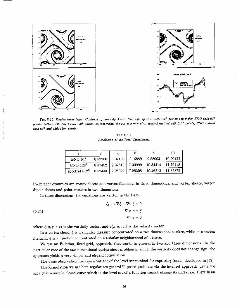
v_
oo _ r, ?,s
u EmI_IB
4o t.I
o
7'lDo|_ soo1:
L_
i.
o,o [ v cuts at t=8, x=pl
Qo .... _o .... _0 *o ,o ie *.o
FIc. 5.10. Double shear lazier. Contours of vorticity, t = 8. Top left: spectral with 5122 points; top right: ENO with 642
points; bottom left: ENO with 1282 points; bottom right: the cut at = = vr of v, spectral method with 5122 points, ENO method
with 642 and with 1282 points.
TABLE 5.2
Resolution of the Total Circulation.
ENO 642
ENO 1282
2 4 6 8 10
0.87300 3.07100 7.16889 9.88063 10.90122
2.97810 7.30999 10.34414 11.794180.87452
0.87433 2.98029 7.28308 10.46212 11.85875
Prominent examples are vortex sheets and vortex filaments in three dimensions, and vortex sheets, vortex
dipole sheets and point vortices in two dimensions.
In three dimensions, the equations are written in the form
6 + vV_ - Vv _ = o
(5.24) V x v =
V.v =0
where _(x, y, z, t) is the vorticity vector, and v(x, y, z, t) is the velocity vector.
In a vortex sheet, _ is a singular measure concentrated on a two dimensional surface, while in a vortex
filament, _ is a function concentrated on a tubular neighborhood of a curve.
We use an Eulerian, fixed grid, approach, that works in general in two and three dimensions. In the
particular case of the two dimensional vortex sheet problem in which the vorticity does not change sign, the
approach yields a very simple and elegant formulation.
The basic observation involves a variant of the level set method for capturing fronts, developed in [59].
The formulation we use here regularizes general ill-posed problems via the level set approach, using the
idea that a simple closed curve which is the level set of a function cannot change its index, i.e. there is an
66
automatictopologicalregularization.Thisisveryhelpfulfornumericalcalculations.Theregularizationisautomaticallyaccomplishedthroughtheuseofdissipativeschemes,whichhastheeffectof addinga smallcurvatureterm(whichvanishesasthegridsizegoestozero)to theevolutionoftheinterface.Theformulationallowsfortopologicalchanges,suchasmergingofsurfaces.
Themainideais to decompose_intoa productof theform
(5.25) _=p(_)_
whereP is a scalar function, typically an approximate 5 function. The variable _ is a scalar function whose
zero level set represents the points where vorticity concentrates, and _/ represents the vorticity strength
vector. This decomposition is performed at time zero and is of course not unique.
The observation is that once a decomposition is found, the following system of equations yields a solution
to the Euler equations, replacing the original set of equations (5.24).
(5.26)
_ot + vVtp = 0
rh + vVr/- Vv r/= 0
V x v = P(_o)r/
V.v=O
These equations have initial conditions
where _0, _0 and P are chosen so that (5.25) holds at time t = 0. Notice that (5.25) and (5.26) imply
that V_ is orthogonal to 7, and div(_) = 0. This is enforced in the initial condition and is maintained
automatically by (5.25) and (5.26).
When P is a distribution, such as a 5 function, approaching P with a sequence of smooth mollifiers P_
yields a sequence of approximating solutions. This is the approach used in numerical calculations, sincc the
5 function can only be represented approximately on a finite grid. The parameter e is usually chosen to be
proportional to the mesh size.
The advantage of this formulation, is that it replaces a possibly singular and unbounded vorticity function
_, by bounded, smooth (at least uniformly Lipschitz) functions _ and _?. Therefore, while it is not feasible
to compute solutions of (5.24) directly, it is very easy to compute solutions of (5.26).
In two dimensions, the vorticity is given by
(o)_= 0
x, y)
and hence the Euler equations arc given by
wt + vVw = 0
=
div(v) = 0
67
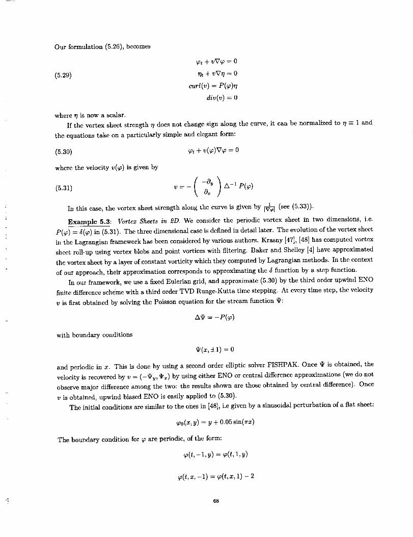
Ourformulation(5.26),becomes
(5.29)
where y is now a scalar.
_t + vVqo = 0
rh + vVr/= 0
curl(v) = P(qo)r l
div(v) = 0
If the vortex sheet strength z/does not change sign along the curve, it can be normalized to r/= 1 and
the equations take on a particularly simple and elegant form:
(5.30)
where the velocity v(_o) is given by
_ot+ v@)V_ = o
-Oy) /X_ _ P(qo)(5.31) v = - O=
In this case, the vortex sheet strength along the curve is given by _ (see (5.33)).
Example 5.3: Vortex Sheets in 2D. We consider the periodic vortex sheet in two dimensions, i.e.
P(_) = d(_) in (5.31). The three dimensional case is defined in detail later. The evolution of the vortex sheet
in the Lagrangian framework has been considered by various authors. Krasny [47], [48] has computed vortex
sheet roll-up usin'g vortex blobs and point vortices with filtering. Baker and Shelley [4] have approximated
the vortex sheet by a layer of constant vorticity which they computed by Lagrangian methods. In the context
of our approach, their approximation corresponds to approximating thc 5 function by a step function.
In our framework, we use a fixed Eulerian grid, and approximate (5.30) by the third order upwind ENO
finite difference scheme with a third order TVD Runge-Kutta time stepping. At every time step, the velocity
v is first obtained by solving the Poisson equation for the stream function g/:
A_ = -P(qo)
with boundary conditions
_,(=,+1) = o
and periodic in x. This is done by using a second order elliptic solver FISHPAK. Once • is obtained, the
velocity is recovered by v = (-@u, _=) by using either ENO or central difference approximations (we do not
observe major difference among the two: the results shown are those obtained by central difference). Once
v is obtained, upwind biased ENO is easily applied to (5.30).
The initial conditions are similar to the ones in [48], i.e given by a sinusoidal perturbation of a flat sheet:
vo(=,y) = y + 0.05sin(,r=)
The boundary condition for _ are periodic, of the form:
v(t, -1, y) = _,(t,1,y)
v(t, =,-1) = _(t, =, 1) - 2
68
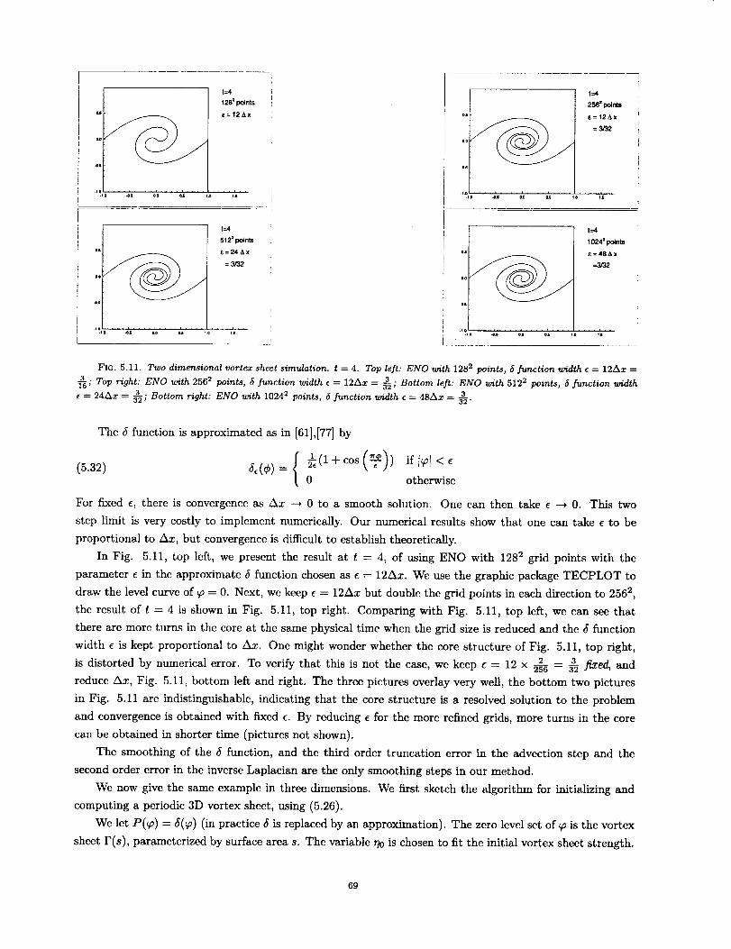
t=4
128 = points
z=12&x
u
ae
_s
t=4
512 = points
_=24&x
=3/32
.o_ oo o.s lo i.s
c_s
t=4
256 _ points
z= 12/,x
= 3132
°f t=4
10248 points
_E=48Ax
--3/32
..,,,lJ
FIO. 5.11. Two dimensional vortex sheet simulation, t = 4. Top left: ENO with 1282 points, 5 function width _ = 12Ax =
3; Top right: ENO with 25@ points, _ function width e = 12Ax = 3; Bottom left: ENO with 512_ points, 5 function width= 24Ax = 3; Bottom right: ENO with 1024_ points, 5 function width e = 48Ax = 3
32"
The _ function is approximated as in [61],[77] by
{ _(l+eos(_)) ifl_ l<c(5.32) _(¢) = 0 otherwise
For fixed e, there is convergence as Ax --, 0 to a smooth solution. One can then take e --* 0. This two
step limit is very costly to implement numerically. Our numerical results show that one can take c to be
proportional to Ax, but convergence is difficult to establish theoretically.
In Fig. 5.11, top left, we present the result at t = 4, of using ENO with 1289_ grid points with the
parameter e in the approximate _ function chosen as e = 12Ax. We use the graphic package TECPLOT to
draw the level curve of _ = 0. Next, we keep e = 12Ax but double the grid points in each direction to 2562,
the result of t = 4 is shown in Fig. 5.11, top right. Comparing with Fig. 5.11, top left, we can see that
there are more turns in the core at the same physical time when the grid size is reduced and the _ function
width e is kept proportional to Ax. One might wonder whether the core structure of Fig. 5.11, top right,
is distorted by numerical error. To verify that this is not the case, we keep e = 12 × _ = 3 fixed, and
reduce Ax, Fig. 5.11, bottom left and right. The three pictures overlay very well, the bottom two pictures
in Fig. 5.11 are indistinguishable, indicating that the core structure is a resolved solution to the problem
and convergence is obtained with fixed c. By reducing e for the more refined grids, more turns in the core
can be obtained in shorter time (pictures not shown).
The smoothing of the J function, and the third order truncation error in the advection step and the
second order error in the inverse Laplacian are the only smoothing steps in our method.
We now give the same example in three dimensions. We first sketch the algorithm for initializing and
computing a periodic 3D vortex sheet, using (5.26).
We let P(qa) = _(qo) (in practice _ is replaced by an approximation). The zero level set of _ is the vortex
sheet F(s), parameterized by surface area s. The variable T0 is chosen to fit the initial vortex sheet strength.
69
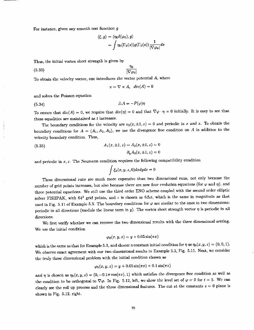
Forinstance,givenanysmoothtestfunctiong
=/ d8
Thus, the initial vortex sheet strength is given by
(5.33) _?olv 01
To obtain the velocity vector, one introduces the vector potential A, where
v = V x A, div(A) = O
and solves the Poisson equation
(5.34) AA = -P(_)_?
To ensure that div(A) = O, we require that divO? ) = 0 and that V_. 77= 0 initially. It is easy to see that
these equalities are maintained as t increases.
The boundary conditions for the velocity are v2(x,+l, z) = 0 and periodic in x and z. To obtain the
boundary conditions for A = (A1,A2,A3), we use the divergence free condition on A in addition to the
velocity boundary condition. Thus,
(5.35) Al(x,-F1, z) = A3(x, ±1, z) = 0
OyA_(x, ±1, z) = 0
and periodic in x, z. The Neumann condition requires the following compatibility condition
/ {2(x, O)dxdydz -- 0Y, Z,
Three dimensional runs are much more expensive than two dimensional runs, not only because the
number of grid points increases, but also because therc are now four evolution equations (for _ and _/), and
three potential equations. We still use the third order ENO scheme coupled with the second order elliptic
solver FISHPAK, with 643 grid points, and e is chosen as 6Ax, which is the same in magnitude as that
used in Fig. 5.11 of Example 5.3. The boundary conditions for _ arc similar to the ones in two dimensions:
periodic in all directions (module thc linear term in y). The vortex sheet strength vector _ is periodic in all
directions.
We first verify whether we can recover the two dimensional results with the three dimensional setting.
We use the initial condition
y, z) = y + 0.05sin( )
which is the same as that for Example 5.3, and choose a constant initial condition for T/as _0(x, y, z) = (0, 0, 1).
We observe exact agreement with our two dimensional results in Example 5.3, Fig. 5.11. Next, we consider
the truly three dimensional problem with the initial condition chosen as
_0(x, y, z) = y + 0.05 sin(rx) + 0.1 sin(lrz)
and 7? is chosen as r/0(x, y, z) = (0,-0.11r cos(rz), 1) which satisfies the divergence free condition as well as
the condition to be orthogonal to V_. In Fig. 5.12, left, wc show the level set of _ = 0 for t = 5. We can
clearly see the roll up process and the three dimensional features. The cut at the constants z = 0 plane is
shown in Fig. 5.12, right.
7O
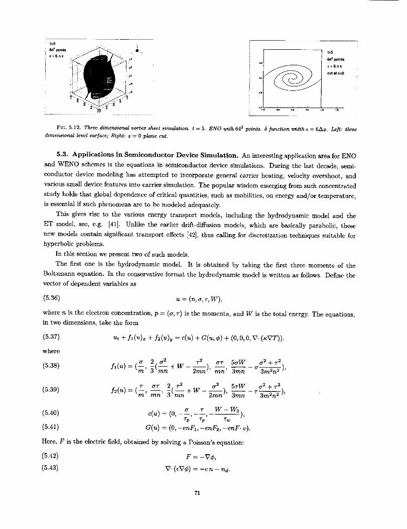
1=5
i 64 _ po_.tS¢=6Ax
' ................................................ "" ..............
t=5
64:' points
¢:6AX
cut at z=O
o.
,0.6
FIG. 5.12. Three dimensional vortex sheet simulation, t = 5. ENO with 643 points. _ function width e = 6Ax. Left: threedimensional level surface; Right: z = 0 plane cut.
5.3. Applications in Semiconductor Device Simulation. An interesting application area for ENO
and WENO schemes is the equations in semiconductor device simulations. During the last decade, semi-
conductor device modeling has attempted to incorporate general carrier heating, velocity overshoot, and
various small device features into carrier simulation. The popular wisdom emerging from such concentrated
study holds that global dependence of critical quantities, such as mobilities, on energy and/or temperature,
is essential if such phenomena are to be modeled adequately.
This gives rise to the various energy transport models, including the hydrodynamic model and the
ET model, see, e.g. [41]. Unlike the earlier drift-diffusion models, which are basically parabolic, these
new models contain significant transport effects [42], thus calling for discretization techniques suitable for
hyperbolic problems.
In this section we present two of such models.
The first one is the hydrodynamic model. It is obtained by taking the first three moments of the
Boltzmann equation. In the conservative format the hydrodynamic model is written as follows. Define the
vector of dependent variables as
(5.36) u = (n, a, r, W),
where n is the electron concentration, p = (a, _-) is the momenta, and W is the total energy. The equations,
in two dimensions, take the form
(5.37)
where
(5.38)
ut + f l (U)x + f2(u)y = c(u) + G(u, ¢) + C0, 0, 0, V. (e_VT)).
a 2(a 2 r 2 ar 5aW a 2+T 2fl(u) = (m' 5 _ + W - _mn) , ran' 3ran a 3--mS-_-n2)'
(5.39)7-
f2(u)=(m ' ar 2(r 2 a2 5rW _2+r2ran' 5 _ + w - 2--_), 3ran T3--_-_-_21'
(5.40) c(u) (0, ° r w-w0
(5A1) G(=) = (0, -_=F_, -enF2, -e_F. _).
Here, F is the electric field, obtained by solving a Poisson's equation:
(5.42) F = -re,
(5.43) V-(eve) = -e n - rid.
71
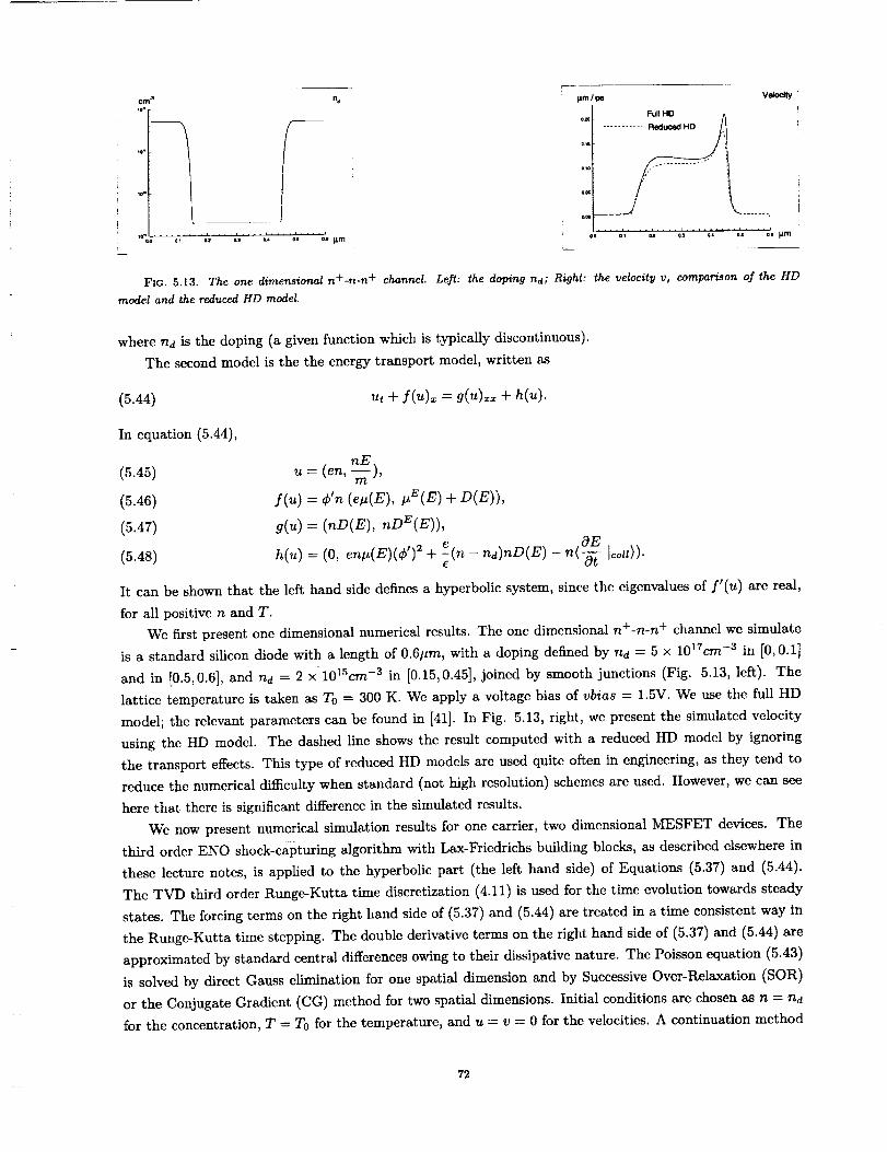
to-
1o-__
I_./_ Vek_Ity
*x F_I HD /_
aa
a* *, " o_ o_' o, U ol I,Lm
FxG. 5.13. The one dimensional n+-n-n + channel. Left: the doping rid; Right: the velocity v, comparison of the HD
model and the reduced HD model.
where na is the doping (a given function which is typically discontinuous).
The second model is the the energy transport model, written as
(5.44)
In equation (5.44),
(5.45)
(5.46)
(5.47)
(5.48)
+ f(u) = g(,,)x, +
nEu = m)'
f(u) = ¢'n (etz(E), #E(E) + D(E)),
g(u) = (nD(E), nDE(E)),
e OE
h(u) = (0, enl_(E)(¢') 2 + _(n - n_)nD(E) - n{-ff{ Icott) ).
It can be shown that the ]eft hand side defines a hyperbolic system, since the eigenvalues of f'(u) are real,
for all positive n and T.
We first present one dimensional numerical results. The one dimensional n+-n-n + channel wc simulate
is a standard silicon diode with a length of 0.6#m, with a doping defined by na = 5 × 10¹⁷c'm -3 in [0,0.1]
and in [0.5,0.6], and na = 2 × 1015cm -3 in [0.15,0.45], joined by smooth junctions (Fig. 5.13, left). The
lattice temperature is taken as To = 300 K. We apply a voltage bias of vbias = 1.5V. We use the full HD
model; the relevant parametcrs can be found in [41]. In Fig. 5.13, right, we present the simulated velocity
using the HD modcl. The dashed line shows the result computed with a reduced HD model by ignoring
the transport effects. This type of reduced HD models are used quite often in engineering, as they tend to
reduce the numerical difficulty when standard (not high resolution) schemes are used. However, we can see
here that there is significant difference in the simulated results.
We now present numerical simulation results for one carrier, two dimensional MESFET devices. The
third order ENO shock-capturing algorithm with Lax-Friedrichs building blocks, as described elsewhere in
these lecture notes, is applied to the hyperbolic part (the left hand side) of Equations (5.37) and (5.44).
The TVD third order Runge-Kutta time discretization (4.11) is used for the time evolution towards steady
states. The forcing terms on the right hand side of (5.37) and (5.44) are treated in a time consistent way in
the Runge-Kutta time stepping. The double derivative terms on the right hand side of (5.37) and (5.44) are
approximated by standard central differences owing to their dissipative nature. The Poisson equation (5.43)
is solved by direct Gauss elimination for one spatial dimension and by Successive Over-Relaxation (SOR)
or the Conjugate Gradient (CG) method for two spatial dimensions. Initial conditions are chosen as n = na
for the concentration, T = To for the temperature, and u = v = 0 for the velocities. A continuation method
72
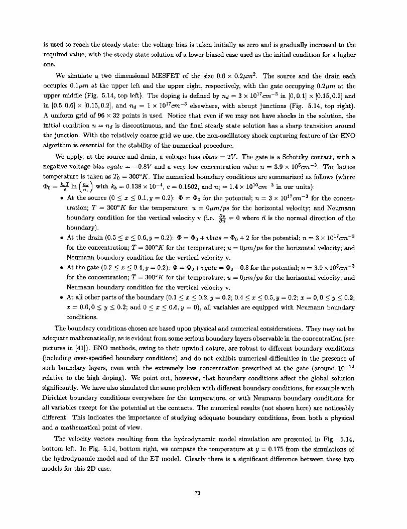
is used to reach the steady state: the voltage bias is taken initially as zero and is gradually increased to the
required value, with the steady state solution of a lower biased case used as the initial condition for a higher
one.
We simulate a two dimensional MESFET of the size 0.6 x 0.2_m 2. The source and the drain each
occupies 0.1#m at the upper left and the upper right, respectively, with the gate occupying 0.2#m at the
upper middle (Fig. 5.14, top left). The doping is defined by nd -- 3 x 1017cm -3 in [0, 0.1] x [0.15,0.2] and
in [0.5,0.6] x [0.15,0.2], and nd= 1 x 1017cm -3 elsewhere, with abrupt junctions (Fig. 5.14, top right).
A uniform grid of 96 x 32 points is used. Notice that even if we may not have shocks in the solution, the
initial condition n -- nd is discontinuous, and the final steady state solution has a sharp transition around
the junction. With the relatively coarse grid we use, the non-oscillatory shock capturing feature of the ENO
algorithm is essential for the stability of the numerical procedure.
We apply, at the source and drain, a voltage bias vbias = 2V. The gate is a Schottky contact, with a
negative voltage bias vgate = -0.8V and a very low concentration value n -- 3.9 x 10Sere -3. The lattice
temperature is taken as To = 300°K. The numerical boundary conditions are summarized as follows (where
(_-_) with kb 0.138 x 10-a, e 0.1602, and n, lax 101°cm -3 in our units):(I)0 ---- in n_ = = =
• At the source (0 < x < 0.1, y = 0.2): ¢ = (I)0 for the potential; n = 3 x 10¹⁷c-_2 -3 for the concen-
tration; T = 300°K for the temperature; u -- O#m/ps for the horizontal velocity; and Neumann
boundary condition for the vertical velocity v (i.e. o, --- 0 where g is the normal direction of the
boundary).
• At the drain (0.5 < x < 0.6, y = 0.2): ¢ -- ¢0 + vbias -- (I)0 + 2 for the potential; n = 3 x 10¹⁷ern -3
for the concentration; T -- 300°K for the temperature; u = O#m/ps for the horizontal velocity; and
Neumann boundary condition for the vertical velocity v.
• At the gate (0.2 < x < 0.4, y = 0.2): _) - _Po+vgate -- _0-0.8 for the potential; n = 3.9 x 10Sere -3
for the concentration; T = 300°K for the temperature; u = O#m/ps for the horizontal velocity; and
Neumann boundary condition for the vertical velocity v.
• At all other parts of the boundary (0.1 < x < 0.2, y = 0.2; 0.4 < x < 0.5,y= 0.2; x = 0,0 < y < 0.2;
x -- 0.6, 0 _< y < 0.2; and 0 < x < 0.6, y -- 0), all variables are equipped with Neumann boundary
conditions.
The boundary conditions chosen are based upon physical and numerical considerations. They may not be
adequate mathematically, as is evident from some serious boundary layers observable in the concentration (see
pictures in [41]). ENO methods, owing to their upwind nature, are robust to different boundary conditions
(including over-specified boundary conditions) and do not exhibit numerical difficulties in the presence of
such boundary layers, even with the extremely low concentration prescribed at the gate (around 10 -12
relative to the high doping). We point out, however, that boundary conditions affect the global solution
significantly. We have also simulated the same problem with different boundary conditions, for example with
Dirichlct boundary conditions everywhere for the temperature, or with Neumann boundary conditions for
all variables except for the potential at the contacts. The numerical results (not shown here) are noticeably
different. This indicates the importance of studying adequate boundary conditions, from both a physical
and a mathematical point of view.
The velocity vectors resulting from the hydrodynamic model simulation are presented in Fig. 5.14,
bottom left. In Fig. 5.14, bottom right, we compare the temperature at y = 0.175 from the simulations of
the hydrodynamic model and of the ET model. Clearly there is a significant difference between these two
models for this 2D case.
73
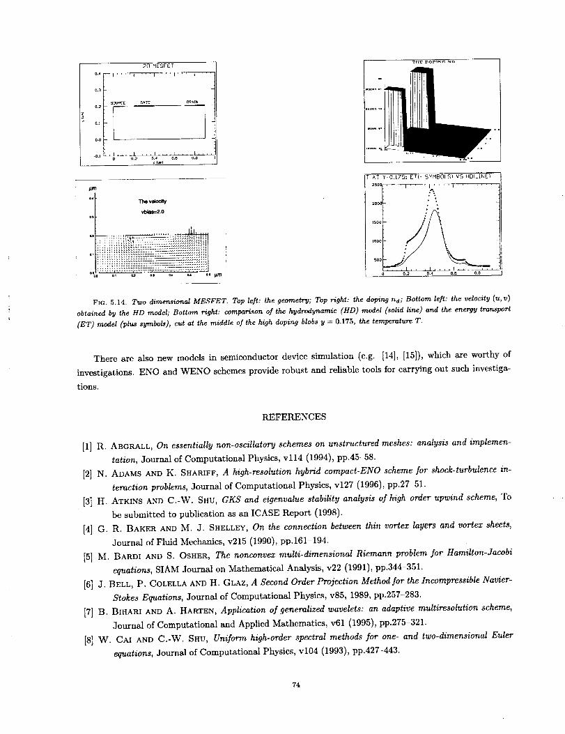
0.4
O.3
0 ..if'
0.1
0.0
"0.1
20 MESFET
o 0.2 o.d o.1_ a,8
_l,m
a,i
Tt'mwlodty
vl:gaw=2.0as
a2_ .................. _ ....
T AT Y-OATS:_.ETU SYMBOLS) VS HIDILINEI 1II
2000_ ,
°°E&iooo
0.2 0.4 O_ 0.8
FIG. 5.14. Two dimensional MESFET. Top left: the geometry; Top right: the dopin 9 ha; Bottom left: the velocity (u,v)
obtained by the HD model; Bottom right: comparison of the hydrodynamic (HD) model (solid line) and the energy transport
(ET) model (plus symbols), cut at the middle of the high doping blobs y = 0.175, the temperature T.
There are also new models in semiconductor device simulation (e.g. [14], [15]), which are worthy of
investigations. ENO and WENO schemes provide robust and reliable tools for carrying out such investiga-
tions.
REFERENCES
[1] R. ABGRALL, On essentially non-oscillatory schemes on unstructured meshes: analysis and implemen-
tation, Journal of Computational Physics, vl14 (1994), pp.45- 58.
[2] N. ADAMS AND K. SHARIFF, A high-resolution hybrid compact-ENO scheme for shock-turbulence in-
teraction problems, Journal of Computational Physics, v127 (1996), pp.27 51.
[3] H. ATKINS AND C.-W. SHU, GKS and eigenvalue stability analysis of high order upwind scheme, To
be submitted to publication as an ICASE Report (1998).
[4] G. R. BAKER AND M. J. SHELLEY, On the connection between thin vortex layers and vortex sheets,
Journal of Fluid Mechanics, v215 (1990), pp.161--194.
[5] M. BARDI AND S. OSHER, The nonconvex multi-dimensional Riemann problem for Hamilton-Jacobi
equations, SIAM Journal on Mathematical Analysis, v22 (1991), pp.344-351.
[6] J. BELL, P. COLELLA AND H. GLAZ, A Second Order Projection Method for the Incompressible Navier-
Stokes Equations, Journal of Computational Physics, v85, 1989, pp.257-283.
[7] B. BZHARI AND A. HARTEN, Application of generalized wavelets: an adaptive multiresolution scheme,
Journal of Computational and Applied Mathematics, v61 (1995), pp.275-321.
[8] W. CAI AND C.-W. SHU, Uniform high-order spectral methods for one- and two-dimensional Euler
equations, Journal of Computational Physics, v104 (1993), pp.427-443.
74
[9] C. CANUTO, M.Y. HUSSAINI, A. QUARTERONI AND T. A. ZANG, Spectral Methods in Fluid Dynamics,
Springer-Verlag, 1988.
[10] M. CARPENTER AND C. KENNEDY, Fourth-order 2N-storage Runge-Kutta schemes, NASA TM 109112,
NASA Langley Research Center, June 1994.
[11] J. CASPER, Finite-volume implementation o] high-order essentially nonoscillatory schemes in two di-
mensions, AIAA Journal, v30 (1992), pp.2829 2835.
[12] J. CASPER AND H. ATKINS, A finite-volume high-order ENO scheme ]or two dimensional hyperbolic
systems, Journal of Computational Physics, vl06 (1993), pp.62 76.
[13] J. CASPER, C.-W. SHU AND H. ATKINS, Comparison of two formulations for high-order accurate
essentially nonoscillatory schemes, AIAA Journal, v32 (1994), pp.1970-1977.
[14] C. CERCIGNANI, I. GAMBA, J. JEROME AND C.-W. SHU, Applicability of the high field model: an
analytical study via asymptotic parameters defining domain decomposition, VLSI Design, to appear.
[15] C. CERCIGNANI, I. GAMBA, J. JEROME AND C.-W. SHU, Applicability of the high field model: a
preliminary numerical study, VLSI Design, to appear.
[16] S. CHRISTOFI, The study o] building blocks ]or ENO schemes, Ph.D. thesis, Division of Applied Math-
ematics, Brown University, September 1995.
[17] B. COCKBURN, Discontinuous Galerkin method, Lecture Notes in Mathematics, CIME Subseries,
Springer-Verlag, to appear.
[18] S. COCKBURN AND C.-W. SHe, TVB Runge-Kutta local projection discontinuous Galerkin finite ele-
ment method for conservation laws II: general framework, Mathematics of Computation, v52 (1989),
pp.411-435.
[19] B. COCKBURN, S.-Y. LIN AND C.-W. SHU, TVB Runge-Kutta local projection discontinuous GaIerkin
finite element method ]or conservation laws III: one dimensional systems, Journal of Computational
Physics, v84 (1989), pp.90 113.
[20] B. COCKBURN, S. Hou AND C.-W. SHU, The Runge-Kutta local projection discontinuous Galerkin
finite element method ]or conservation laws IV: the multidimensional case, Mathematics of Compu-
tation, v54 (1990), pp.545 581.
[21] B. COCKBURN AND C.-W. SHU, The Runge-Kutta discontinuous Galerkin method ]or conservation
laws V: multidimensional systems, preprint. Submitted to Journal of Computational Physics.
[22] M. CRANDALL AND P. LIONS, Viscosity solutions of Hamilton-Jacobi equations, Transactions of the
American Mathematical Society, v277 (1983), pp.l-42.
[23] M. CRANDALL AND P. LIONS, Two approximations of solutions of Hamilton-Jacobi equations, Mathe-
matics of Computation, v43 (1984), pp.l-19.
[24] A. DOLEZAL AND S. WONG, Relativistic hydrodynamics and essentially non-oscillatory shock capturing
schemes, Journal of Computational Physics, v120 (1995), pp.266-277.
[25] R. DONAT AND A. MARQUINA, Capturing shock reflections: an improved flux formula, Journal of
Computational Physics, v125 (1996), pp.42-58.
[26] W. E AND C.-W. SHU, A numerical resolution study o] high order essentially non-oscillatory schemes
applied to incompressible flow, Journal of Computational Physics, vll0 (1994), pp.39 46.
[27] G. ERLEBACHER, Y. HUSSAINI AND C.-W. SHU, Interaction of a shock with a longitudinal vortex,
Journal of Fluid Mechanics, v337 (1997), pp.129 153.
[28] E. FATEMI, J. JEROME AND S. OSHER, Solution of the hydrodynamic device model using high order non-
oscillatory shock capturing algorithms, IEEE Transactions on Computer-Aided Design of Integrated
75
CircuitsandSystems,vl0 (1991),pp.232244.[29]S. GOTTLIEBANDC.-W. SHU, Total variation diminishing Runge-Kutta schemes, Mathematics of
Computation, to appear.
[30] B. GUSTAFSSON, H.-O. KREISS AND A. SUNDSTROM, Stability theory of difference approximations for
mixed initial boundary value problems, II, Mathematics of Computation, v26 (1972), pp.649 686.
[31] E. HARABETIAN, S. OSHER AND C.-W. SHU, An Eulerian approach for vortex motion using a level
set reguIarization procedure, Journal of Computational Physics, v127 (1996), pp.15-26.
[32] A. HARTEN, The artificial compression method for computation of shocks and contact discontinuities
III: self-adjusting hybrid schemes, Mathematics of Computation, v32 (1978), pp.363-389.
[33] A. HARTEN, High resolution schemes for hyperbolic conservation laws, Journal of Computational
Physics, v49 (1983), pp.357-393.
[34] A. HARTEN, Preliminary results on the extension of ENO schemes to two dimensional problems, in
Proceedings of the International Conference on Hyperbolic Problems, Saint-Etienne, 1986.
[35] A. HARTEN, ENO schemes with subcell resolution, Journal of Computational Physics, v83 (1989),
pp.148 184.
[36] A. HARTEN, J. HYMAN AND P. LAX, On finite difference approximations and entropy conditions for
shocks, Communications in Pure and Applied Mathematics, v29 (1976), pp.297-322.
[37] A. HARTEN AND S. OSHER, Uniformly high-order accurate non-oscillatory schemes, I, SIAM Journal
on Numerical Analysis, v24 (1987), pp.279 309.
[38] A. HARTEN, B. ENGQUIST, S. OSHER AND S. CHAKRAVARTHY, Uniformly high order essentially non-
oscillatory schemes, III, Journal of Computational Physics, v71 (1987), pp.231-303.
[39] A. HARTEN, S. OSHER, B. ENGQUIST AND S. CIJAKRAVARTHY, Some results on uniformly high order
accurate essentially non-oscillatory schemes, Applied Numerical Mathematics, v2 (1986), pp.347-
377.
[40] A. ISKE AND T. SONER, On the structure of function spaces in optimal recovery of point functionals
for ENO-schemes by radial basis functions, Numerische Mathematik, v74 (1996), pp.177 201.
[41] J. JEROME AND C.-W. SHU, Energy models for one-carrier transport in semiconductor devices, in IMA
Volumes in Mathematics and Its Applications, v59, W. Coughran, J. Cole, P. Lloyd and J. White,
editors, Springer-Verlag, 1994, pp.185 207.
[42] J. JEROME AND C.-W. SHU, Transport effects and characteristic modes in the modeling and simulation
of submicron devices, IEEE Transactions on Computer-Aided Design of Integrated Circuits and
Systems, v14 (1995), pp.917 923.
[43] G. JIANG AND C.-W. SHU, Efficient implementation of weighted ENO schemes, Journal of Computa-
tional Physics, v126 (1996), pp.202-228.
[44] G. JIANC AND S.-H. YU, Discrete shocks for finite difference approximations to scalar conservation
laws, SIAM Journal on Numerical Analysis, to appear.
[45] G. JIANC AND D. PENG, Weighted ENO schemes for Hamilton-Jacobi equations, SIAM Journal on
Scientific Computing, submitted.
[46] D. A. KOPRIVA, A Practical Assessment of Spectral Accuracy for Hyperbolic Problems with Disconti-
nuities, Journal of Scientific Computing, v2, 1987, pp.249 262.
[47] R. KRASNY, A study of singularity formation in a vortex sheet by the point-vortex approximation,
Journal of Fluid Mechanics, v167 (1986), pp.65-93.
[48] R. KRASNY, Desingularization of periodic vortex sheet roll-up, Journal of Computational Physics, v65
76
(1986),pp.292-313.[49]F. LADEINDE,E. O'BRIEN,X. CAI ANDW. LIU,Advection by polytropic compressible turbulence,
Physics of Fluids, v7 (1995), pp.2848 2857.
[50] F. LAFON AND S. OSHER, High-order 2-dimensional nonosciUatory methods for solving Hamilton-Jacobi
scalar equations, Journal of Computational Physics, v123 (1996), pp.235 253.
[51] P. D. LAX AND B. WENDROFF, Systems of conservation laws, Communications in Pure and Applied
Mathematics, vl3 (1960), pp.217-237.
[52] R. J. LEVEQUE, Numerical Methods for Conservation Laws, Birkhauser Verlag, Basel, 1990.
[53] X.-D. LIU, S. OSHER AND T. CHAN, Weighted essentially nonoscillatory schemes, Journal of Compu-
tational Physics, vl15 (1994), pp.200-212.
[54] X.°D. LIU AND S. OSHER, Convex ENO high order multi-dimensional schemes without field by field
decomposition or staggered grids, UCLA CAM (Computational and Applied Mathematics) Report
No. 97-26. Journal of Computational Physics, to appear.
[55] A. MAJDA, J. MCDONOUGH AND S. OSHER, The Fourier Method for Nonsmooth Initial Data, Math-
ematics of Computation, v32, 1978, pp.1041 1081.
[56] H. NESSYAHU AND E. TADMOR, Non-oscillatory central differencing for hyperbolic conservation laws,
Journal of Computational Physics, v87 (1990), pp.408-463.
[57] S. OSHER, Riemann solvers, the entropy condition, and difference approximations, SIAM Journal on
Numerical Analysis, v21 (1984), pp.217-235.
[58] S. OSHER AND S. CHAKRAVARTHY, Upwind schemes and boundary conditions with applications to Euler
equations in general geometries, Journal of Computational Physics, v50 (1983), pp.447-481.
[59] S. OSHER AND J. SETHIAN, Fronts propagating with curvature-dependent spee& algorithms based on
Hamilton-Jacobi formulation, Journal of Computational Physics, v79 (1988), pp.12 49.
[60] S. OSHER AND C.-W. SHU, High-order essentially nonoscillatory schemes for Hamilton-Jacobi equa-
tions, SIAM Journal on Numerical Analysis, v28 (1991), pp.907-922.
[61] C.S. PESKIN, Numerical analysis of blood flow in the heart, Journal of Computational Physics, v25
(1977),pp220 252[62] P. L. ROE, Approximate Riemann solvers, parameter vectors, and difference schemes, Journal of Com-
putational Physics, v43 (1981), pp.357-372.
[63] A. ROGERSON AND E. MEIBERG, A numerical study of the convergence properties of ENO schemes.
Journal of Scientific Computing, v5 (1990), pp.151 167.
[64] J. SETHIAN, Level Set Methods: Evolving Interfaces in Geometry, Fluid Dynamics, Computer Vision,
and Material Science, Cambridge Monographs on Applied and Computational Mathematics, Cam-
bridge University Press, New York, New York, 1996.
[65] C.-W. SHU, TVB uniformly high order schemes for conservation laws, Mathematics of Computation,
v49 (1987), pp.105 121.
[66] C.-W. SHU, Total-Variation-Diminishing time discretizations, SIAM Journal on Scientific and Statis-
tical Computing, v9 (1988), pp.1073 1084.
[67] C.-W. SHU, Numerical experiments on the accuracy of ENO and modified ENO schemes, Journal of
Scientific Computing, v5 (1990), pp.127-149.
[68] C.-W. SHU, Preface to the republication of "Uniform high order essentially non-oscillatory schemes,
III," by Harten, Engquist, Osher, and Chakravarthy, Journal of Computational Physics, vl31 (1997),
pp.1 2.
77
[69]C.-W. SHU AND S. OSHER, Efficient implementation of essentially non-oscillatory shock capturing
schemes, Journal of Computational Physics, v77 (1988), pp.439-471.
[70] C.-W. SHU AND S. OSHER, Efficient implementation of essentially non-oscillatory shock capturing
schemes II, Journal of Computational Physics, v83 (1989), pp.32-78.
[71] C.-W. SHU, T.A. ZANG, G. ERLEBACHER, D. WHITAKER, AND S. OSHER, High order ENO schemes
applied to two- and three- dimensional compressible flow, Applied Numerical Mathematics, v9 (1992),
pp.45-71.
[72] C.-W. SHU AND Y. ZENG, High order essentially non-oscillatory scheme for viscoelasticity with fading
memory, Quarterly of Applied Mathematics, to appear.
[73] K. SIDDIQI, B. KIMIA AND C.-W. SHU, Geometric shock-capturing ENO schemes for subpixel in-
terpolation, computation and curve evolution, Computer Vision Graphics and Image Processing:
Graphical Models and Image Processing (CVGIP:GMIP), to appear.
[74] J. SMOLLER, Shock Waves and Reaction-Diffusion Equations, Springer-Verlag, New York, 1983.
[75] G. A. SOD, Numerical Methods in Fluid Dynamics, Cambridge University Press, Cambridge, 1985.
[76] J. STRIKWERDA, Initial boundary value problems for the method of lines, Journal of Computational
Physics, v34 (1980), pp.94-107.
[77] M. SUSSMAN, P. SMEREKA, AND S. OSHER, A level set approach for computing solutions to incom-
pressible two phase flow, Journal of Computational Physics, v114 (1994), pp.146-159.
[78] P. K. SWEBY, High resolution schemes using flux limiters for hyperbolic conservation laws, SIAM
Journal on Numerical Analysis, v21 (1984), pp.995-1011.
[79] B. VAN LEER, Towards the ultimate conservative difference scheme V. A second order sequel to Go-
dunov's method, Journal of Computational Physics, v32 (1979), pp. 101-136.
[80] F. WALSTEIJN, Robust numerical methods for 2D turbulence, Journal of Computational Physics, vl14
(1994), pp.129-145.
[81] J.H. WILLIAMSON, Low-storage Runge-Kutta schemes, Journal of Computational Physics, v35 (1980),
pp.48 56.
[82] P. WOODWARD AND P. COLELLA, The numerical simulation of two-dimensional fluid flow with strong
shocks, Journal of Computational Physics, v54, 1984, pp.115-173.
[83] H. YANG, An artificial compression method for ENO schemes, the slope modification method, Journal
of Computational Physics, v89 (1990), pp.125-160.
78

Form ApprovedREPORT DOCUMENTATION PAGE OMB No. 0704-0188
Public reporting burden for this collection of information is estimated to average 1 hour per response, including the time for reviewing instructions, searching existing data sources,
&athedng and maintaTning the data needed, and completing and reviewing the collection of information. Send comments regarding this burden estimate or any other aspect of this
collc_--t;on of inform.at;on, inclucI.Tng suggestions for reducing this burden, to Washington Headquarters Services, Directorate for Information Operations and Reports, 1215 JefFerson
Da_s H4ghway, Suite 1204, Arhngton, VA 22202-4302. and to the Office of" Management and Budget, Paperwork Reduction Project (0704-0188), Washington, DC 20503.
|. AGENCY USE ONLY(Leave blank) 2, REPORT DATE 3. REPORT TYPE AND DATES COVERED
November 1997 Contractor Report
4. TITLE AND SUBTITLE 5. FUNDING NUMBERS
Essentially Non-Oscillatory and Weighted Essentially Non-Oscillatory
Schemes for Hyperbolic Conservation Laws
6. AUTHOR(S)
Chi-Wang Shu
7. PERFORMING ORGANIZATION NAME(S) AND ADDRESS(ES)
Institute for Computer Applications in Science and Engineering
Mail Stop 403, NASA Langley Research Center
Hampton, VA 23681-0001
9. SPONSORING/MONITORING AGENCY NAME(S) AND ADDRESS(ES)
National Aeronautics and Space Administration
Langley Research Center
Hampton, VA 23681-2199
C NAS1-19480
WU 505-90-52-01
8. PERFORMING ORGANIZATIONREPORT NUMBER
ICASE Report No. 97-65
10. SPONSORING/MONITORINGAGENCY REPORT NUMBER
NASA CR-97-206253
ICASE Report No. 97-65
11. SUPPLEMENTARY NOTES
Langley Technical Monitor: Dennis M. Bushnell
Final Report
To appear in Lecture Notes in Mathematics, CIME Subseries, Springer-Verlag
12a. DISTRIBUTION/AVAILABILITY STATEMENT 12b. DISTRIBUTION CODE
Unclassified-Unlimited
Subject Category 64
Distribution: Nonstandard
Availability: NASA-CASI (301)621-0390
13. ABSTRACT (Maximum 200 words)
In these lecture notes we describc the construction, analysis, and application of ENO (Essentially Non-Oscillatory)
and WENO (Weighted Essentially Non-Oscillatory) schemes for hyperbolic conservation laws and related Hamilton-
3acobi equations. ENO and WENO schemes are high order accurate finite difference schemes designed for problems
with piecewise smooth solutions containing discontinuities. The key idea lies at the approximation level, where a
nonlinear adaptive procedure is used to automatically choose the locally smoothest stencil, hence avoiding crossing
discontinuities in the interpolation procedure as much as possible. ENO and WENO schemes have been quite suc-
cessful in applications, especially for problems containing both shocks and complicated smooth solution structures,
such as compressible turbulence simulations and aeroacoustics.
These lecture notes are basically self-contained. It is our hope that with these notes and with the help of the
quoted references, the reader can understand the algorithms and code them up for applications. Sample codes arealso available from the author.
14. SUBJECT TERMS
essentially non-oscillatory, conservation laws, high order accuracy
17. SECURITY CLASSIFICATION
OF REPORTUnclassified
_ISN 7540-01-280-5500
18. SECURITY CLASSIFICATION 19, SECURITY CLASSIFICATION
OF THIS PAGE OF ABSTRACTUnclassified
15. NUMBER OF PAGES
83
16. PRICE CODE
AO_20. LIMITATION
OF ABSTRACT
i
Standard Form 298(Rev. 2-89)Prescribedby ANSI Std. Z39-18298-102