Embed Size (px)
Citation preview
NASA Contractor Report 4531
Three-Dimensional
Boundary-Layer Program
(BL3D) for Swept Subsonic
or Supersonic Wings
With Application to
Laminar Flow Control
Venkit Iyer
ViGYAN, Inc.
Hampton, Virginia
Prepared for
Langley Research Center
under Contract NASl-19672
National Aeronautics and
Space Administration
Office of Management
Scientific and Technical
Information Program
1993
i'np.o
p4I
.,1.
Z
UlrO
imw
O
¢n
,<QZ3Z 14. _ 0
0 3.Jb.4 _.,_ I,L.
Z_W ,,,J Z '<
I EW< m
,-I uJ _-41.-- O_
,COP- _ U
Z C3 ::¢ _ C)
0
0
4-
:E
https://ntrs.nasa.gov/search.jsp?R=19940008600 2020-04-02T12:19:01+00:00Z


Summary
This report deals with the theory, formulation, and solution of compressible three-
dimensional boundary-layer equations with applications to general swept subsonic or
supersonic wings in laminar flow. A number of modifications and new features are
incorporated, based on an earlier general procedure described in NASA CR 4269, Jan.
1990. A more efficient algorithm has been employed, and overall improvements have
been made that result in a user-friendly computer code. An interface routine is presented
that uses the inviscid Euler solutions as input. Code modifications are implemented for
application in laminar flow control design applications. Output of solution profiles and
quantities required in boundary-layer stability analysis is included. Conversion routines
to compare results with Navier-Stokes profiles are also presented.
This report is a stand-alone document that provides all the necessary details for
numerical calculation of three-dimensional swept-wing boundary layers. Examples of
applications and validation with thin-layer Navier-Stokes solutions are presented. A
user's manual is included as an appendix.
Keywords
Boundary layer
Compressible flow
Laminar flow control
Transition prediction
Swept-wing flow
iii PRECF.._I_IG PAGE BLANK NOT FILMED

Table of Contents
Summary
Nomenclature
1.
2.
.
,
.
INTRODUCTION
FORMULATION
2.1 Three-Dimensional Boundary-Layer Coordinates
2.2 Three-Dimensional Boundary-Layer Equations
2.3 Transformation
2.4 Transformed Equations
2.5 Quasi-Two-Dimensional Equations for Initial
Conditions
2.6 Equations in Vector Form
DISCRETIZATION
3.1 Differencing Formulas
3.2 Linearized System at (i,j)
3.3 Boundary Conditions
3.4 Discretization in the (i,j) directions
INVISCID INTERFACE
4.1 Attachment-Line Relocation
4.2 Edge Values by Interpolation
4.3 Edge Values From BL-EDGE Equations
BL3D EXAMPLE CASES
5.1
5.2
5.3
5.4
5.5
5.6
5.7
Geometry and Conditions for Case 1
Euler Solution for Case 1
Euler - BL3D Interface for Case 1
BL3D Solution for Case 1
BL3D Results for Case 1
Results With Suction for Case 1
Geometry and Conditions for Case 2
Page
iii
vii
1
3
3
6
9
11
14
17
21
21
22
24
28
30
31
32
32
34
34
35
36
38
40
42
42
V
PRECEDING PAGE FJLArJ,X _j'3.,T FtLMt_.L,_

Euler Solution and BL3D Interface for Case 2
BL3D Solution for Case 2
43
43
REFERENCES 45
FIGURES 46
APPENDIX A
Coefficients of the Linearized System of Compressible Three-DimensionalBoundary-Layer Equations Discretized With a Fourth-Order Pade Formula
A-1toA-7
APPENDIX B
User's Manual for the BL3D ProgramB-1toB-26

Nomenclature
A1, A2, A3, A4
al_ a2_ a3
a kl,rn
Bi, i = 1,6
/)i, i = 3, 6
/)3,bl, b2, b3,
b4, b5
bk/,m
Ci, i = 1,6
Ci, i = 3, 6
d4,d GG a, C24,C25,C26, C34, C35,
G6CsxDi, i = 1, 5
O3,b4
dsl, ds2
El, i = 1,4F
ffeG
g12
H
HLhb h2
h_I
i,j,kke
k_L
coefficients in the transformed continuity equation (see eqs. (47)-(50))
coefficients in the (-direction differencing formula (see eqs.(129)-(130))
diagonal elements of the linear system given by eq. (101) or (108)
coefficients in the transformed ( momentum equation (see eqs.(55)-(60))coefficients
coefficients
(see eq. (91))
(see eq. (94))
coefficients in the q-direction differencing formula(see eqs. (131)-(133))
superdiagonal elements of the linear system given by eq. (101) or(lO8)coefficients in the transformed r/momentum equation (see eqs.(62)-(67))
coefficients (see eq. (92))
coefficients (see eq. (95))
pressure coefficient
metric coefficients (see eqs. (6)-(12))
skin-friction coefficient in x direction normalized with free-stream values
coefficients in the transformed energy equation (see eqs. (69)-(70))coefficients (see eq. (96))
incremental arc lengths, nondimensional, in the x and y directions (seeeqs. (4)-(5))
coefficients (see eq. (87))u/u_
an arbitrary function
v/v_
metric coefficient (see eq. (3))
total enthalpy, nondimensional (see eq. (24))
free-stream total enthalpy, dimensional (see eq. (23))
metric coefficient (see eqs. (1)-(2))
metric term (see eq. (8))
Heindices in the (, r/, and ( directions
index k that corresponds to the boundary-layer edge
factor for stretching the grid in the _ direction (see eq. (128))
vii
L*I
M
M_
t/X,
nxlim, nylim
P
Pr
PLQq
qs
qwR*
RecF
Reoo
Re 0
[s]Sl, $2
T
TLU*
C.X9
U l, V I, W l
Us, l_s
Vr
W
(v
Co
x, y, z
ak ilk @, 6k
7
¢
reference length, dimensional
I/Pr
c¢free-stream Mach number
maximum number of boundary-layer grid points in x and y directions
limits set on _, ny to restrict computation to a smaller region
static pressure, nondimensionallaminar Prandtl number
free-stream pressure, dimensional
vector (see eq. (85))absolute velocity, nondimensional (see eq. (25))
normalized suction rate defined as qs = (pawl)/(pooU=)
wall heat flux, dimensional
gas constant
crossflow Reynolds number (see eq. (138))
free-stream Reynolds number, based on reference length L_ (see eq.
(29))momentum-thickness Reynolds number (see eq. (139))
residual, right-hand side of equation (108)
solution vector at location (i, j)
nondimensional arc lengths in the x and y directions (see eqs. (4)-(5))
temperature, nondimensionalfree-stream temperature, dimensional
free-stream velocity, dimensionalvelocities in streamwise and spanwise directions, nondimensional
velocities, nondimensional, in Cartesian coordinate directions
boundary-layer velocities along and orthogonal to the edge streamline
reference velocity for vtransformed normal velocity (see eqs. (44)-(45))
scaled normal velocity (see eq. (28))surface-normal velocity, nondimensional
boundary-layer coordinates in streamwise, spanwise, and normal
directions, nondimensionalCartesian coordinates, nondimensional
stretched boundary-layer normal coordinate (see eq. (27))
elements of block tridiagonal system (see eqs. (122)-(t24))
angle between x- and y-coordinate linesratio of specific heats
step size in ( (see eq. (110))
transformed normal coordinate (see eq. (36))
viii

_*0.1
0
A
AO, A1, /_2, A3
#/]
p
XI_ X2_ X3
¢, ¢1, ¢2, ¢3
ff)W
Cq
_at
Subscripts:
e
k=l
k = ke
m_
r
w
x, y, z
_,_,(
1,2
Superscripts:
!
t
n
T
prefix used to indicate change in a solution vector or solution vectorelement at iteration level n and at location (i, j) (see eq. (105), for
example)
boundary-layer thickness, dimensional, at which v, reduces to 10
percent of its maximum valuetransformed boundary-layer surface coordinates
(p lp)sweep angle
coefficients (see eq. (97))
absolute viscosity, nondimensional
kinematic viscosity, nondimensional
density, nondimensional
x/Pe#eSlUe
coefficients (see eq. (87))surface partial derivative functions (see eqs. (14)-(17))
coefficient in normal velocity transformation (see eq. (115))
coefficient in wall heat flux transformation (see eq. (118))
relaxation parameterrelaxation parameter for attachment-line iteration
factor used in finite differencing in ( direction
boundary-layer edgeat the wall
at boundary-layer edgemaximumreference value
wall quantity
partial derivatives in x, y, and z directionspartial derivatives in _, 7/, and ¢ directions
free-stream quantity
x and y directions
dimensional quantityCartesian coordinate (as in x', y', z')
partial derivative in ( (except for x', y', z')iteration number
transpose
ix
Abbreviations:
BL
BL3D
INV
L
LISW
LHS
NS
RHS
Z
Boundary layer
Boundary layer three dimensionalInviscid
Left-pointing
Locally infinite swept wingLeft-hand side
Navier-Stokes
Right-hand side
Zig-zag

1. INTRODUCTION
A renewed interest has developed in the design of wings with extensive lengths of
laminar flow in the subsonic and supersonic regimes. Design for laminar flow by passive
or active means is a multiparameter optimization problem that involves such variables as
surface pressure gradients, leading-edge radius, sweep, suction rates, and free-stream
conditions. To aid in the design process, a reliable computational procedure is needed
to predict boundary-layer stability. An important part of this computational prediction is
the accurate generation of smooth mean-flow profiles. This report addresses the issue
of generating these profiles.
Two options are available for mean-flow prediction. The first one is the use of an
accurate thin-layer Navier-Stokes solver in which particular attention is paid to such
issues as grid resolution and numerical dissipation. However, for repeated preliminary
design calculations, the Navier-Stokes solution is expensive. The second option is
the use of an accurate boundary-layer method coupled with an inviscid Euler solution,
which is particularly attractive for experimentation with different pressure and suction
distributions.
This report deals with the theory, formulation, and solution of compressible three-
dimensional boundary-layer equations, with specific reference to general swept subsonic
or supersonic wings in laminar flow. A number of modifications and new features are
incorporated from an earlier general procedure described in NASA CR 4269, Jan. 1990
(i.e., ref. 1; see also ref. 2). However, the present report is a stand-alone document
that provides all of the necessary details for numerical calculation of three-dimensional
swept-wing boundary layers.
The modifications to the original procedure provide a more efficient algorithm. The

solution scheme has been modified to solve the continuity, energy, and momentum equa-
tions simultaneously, with iterative update of nonlinear terms. Streamwise and spanwise
differencing schemes have been modified to ensure that the boundary-layer solution
is consistent with the boundary-layer-edge boundary conditions. Overall improvements
have been made that result in a more user-friendly computer code. An interface rou-
tine has been developed to use the Euler solutions as input. Code modifications have
been implemented for application in laminar flow control design. The modified code also
provides the output of profiles and quantities that are required in boundary-layer stability
analysis. Conversion routines that enable one to compare the boundary-layer solution
profiles with Navier-Stokes solution profiles are also provided.
Two applications of the code are presented: a subsonic case and a supersonic
case. For the subsonic case, validations with the thin-layer Navier-Stokes solutions are
presented. Detailed comparisons are made of the solution profiles and other boundary-
layer properties. For the supersonic case, comparisons are given of the present code
with a conical swept wing boundary-layer code developed by Kaups and Cebeci (ref. 3).
A user's manual is included as an appendix to this report. The complete program
package is archived in the NASA Langley computer system mass storage and can be
made available per individual request.
2. FORMULATION
2.1 Three-Dimensional Boundary-Layer Coordinates
We start with the definition of the surface-oriented curvilinear nonorthogonal coordi-
nates used in the three-dimensional boundary-layer equations.
Let us assume that the surface of interest is defined in terms of Cartesian coordinates
(x'*, y'*, z'*) in dimensional units (see Figure l(a)). The free-stream quantities are
(M_, P_o, T*) with a corresponding free-stream velocity U_o.
The body coordinates are normalized with a reference length L_o; the Cartesian
components of velocity (u'*, v'*, w'*) are normalized by the reference velocity U%. The
resulting normalized coordinates are ( x', y', z_), and the normalized velocity components
are ( _', v', w'). (See Figure 1(b).) The normalization of other flow quantities is discussed
in the next section.
The boundary-layer coordinates are defined in the two surface directions x and y,
where x is the predominant streamwise direction and y is the general spanwise direction
(not necessarily along the constant percent chord direction for a wing). The coordinate z
is mutually perpendicular to both z and y. The coordinates x and y are surface conforming,
but do not need to be measured as surface arc lengths. For example, for the case
of the attachment-line flow on a swept wing, the boundary-layer coordinate y may be
defined along the attachment line on the surface, but can be expressed as distance
in the spanwise direction perpendicular to the chord. The coordinates x and y can
also be normalized to the (0, l) range in the computational domain. The three basic
metric quantities (hi, h.2, gl_) defined later in this section characterize the stretching and
shearing of the physical grid into the computational grid.
The grid line x = 0 coincides with the starting location of the boundary layer as

shown in Figure 1(c) (in this case, the attachment line of a swept wing). The choice of
z = 0 is important because the system of equations becomes singular at the boundary-
layer origination point, and a special set of equations must be solved here to initialize
the solution.
The transformation of quantities from the (x I, yl z') to the (x, #, z) system is deter-
! ! Imined by the set of six partial derivatives (x_, y_, z=, xy, yy, z_y). Note that in boundary-
layer theory, the planes where z = constant are assumed to be parallel to the surface,
which means that the surface partial derivatives are sufficient to characterize the trans-
formation from one system to another. These partial derivatives enter into the three-
dimensional boundary-layer equations via the three metric quantities (hi, h2, g12) de-
fined as
h_ .= V/(_,)_+ (y,)_ + (z,) _ (1)
h2= + + (2)
I ! 1 I I lg12 = hl h2 cos fl = XxXy -F YxYy + zxzy (3)
The metric coefficients h_ and h2 represent the stretching in the two surface coordinate
directions with reference to the physical grid. The nondimensional surface arc lengths
in the two directions sl and s2 are defined by the two incremental relations
dsa = hi dx (4)
ds2 = h2 dy (5)

Further, the quantity 912/hlh2 is the cosine of the angle/_ between the two coordinates
x and y. The additional coefficients, based on hi, h2 and 912, are defined as
V/ 2 ) 2C13 = hlh5 - 912 (6)
024 = 919_, f912 i }C13 [_1 hlx @ hly -- h-_ gl2x(7)
C25 - C231.{hshly - 2912h2x}," hs = hlh2 l+ _hih2j
hi { g12 h2y } (9)C26 -- C23 912y -- h2h2._ h2
h2{ 912 hlx}C34 = C2-.-_,3 gl2x - hlhly hi(10)
1
C35 -- C123 {]_sh2x -- 2912hly} (11)
, }, g12 _.ql_ h2y + h2x -- -- gl2y (12)636 -- 023 1, ].12 h2
The transformation of velocities from (u', v', u,r) to (u, v, d,) is accomplished by
the inversion of the system given below. Note that 5, is the symbol used for the
nondimensional surface-normal velocity; the symbol _v is reserved for later use as
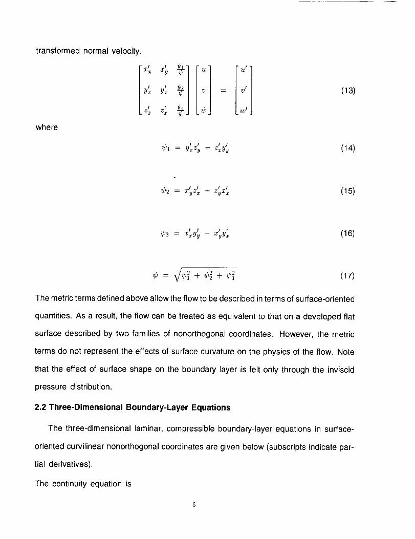
transformed normal velocity.
where
1X x
y,
IZ x
xy ¢ u
I
z_ ¢ _ _wJ
U t
W I
(13)
t_ 1 I i i ry_ zu (14)--__ _ Zxyy
I .,,I ! l_2 _ Xy_'x -- ZyXx (15)
= Xxyy -- Xyy x (16)
V/ ,,/,2 (17)¢ = + + 3
The metric terms defined above allow the flow to be described in terms of surface-oriented
quantities. As a result, the flow can be treated as equivalent to that on a developed flat
surface described by two families of nonorthogonal coordinates. However, the metric
terms do not represent the effects of surface curvature on the physics of the flow. Note
that the effect of surface shape on the boundary layer is felt only through the inviscid
pressure distribution.
2.2 Three-Dimensional Boundary-Layer Equations
The three-dimensional laminar, compressible boundary-layer equations in surface-
oriented curvilinear nonorthogonal coordinates are given below (subscripts indicate par-
tial derivatives).
The continuity equation is

hi pu + k, h,2 pv + (Clap =x Y
(18)
The momentum equation in the x direction is
)fl llx -'}- -_21ty + I_lik + C24 l/2 --[- C25 ttv -it- C26 v 2
hlh_ hlgl2 ) 1
The momentum equation in the y direction is
-(19)
p Vx -'[- _2 Vy + tVV_ -t- C34u 2 --l- C35 uv -t- C361)2
)1{'h2912 p, h2h2 py "/M2
(20)
The energy equation is written in terms of the nondimensional total enthalpy H. When
perfect gas and constant specific heats are assumed, the dimensional total enthalpy I-I*
is defined as
H* R*_ T* + 1 q,Z (21)
where
,2 = u,,Z + v,*2 + w_*2 _ u .2 + v .2 + 2u'v'cos/3 (22)q
The nondimensional total enthalpy H = H*/H_ is based on the reference value
1R*7 T_ + U_ (23)
H* - -_-1
which results in the definition
T + 0.5(_/-1)M 2qz
1 + 0.5(3 _ - 1) ML(24)

with T = T*/T_o and
q2 = u 2 + v 2 + 2uvcosfl (25)
The resulting energy equation is
[. .(1) ]p(uHx + vHv + (vIIs) = _r.rH_ + 2 1______.r (q2);
In the equations above, _ and t_ are stretched quantities with a free-stream Reynolds
number scaling applied as
_" = _"_ (27)
where
,b = _ RV/-R--_ (28)
Redo * * * (29)= ULL_/._
Other variables are normalized as p* by p;_', T* by T2_; P* by P_; and t_* by u_.* The
equation of state is then written as
P = p T (30)
The pressure coefficient can be written as
2(P- 1)C,,--/ML
The variation of viscosity with temperature is modeled by the Sutherland law as
. /_,*T *1.5,a -
T* + T*
'7'* = 198.6°R = 110.33 K
(31)
(32)
tt* = 2.27x 10 -s lb-secft 2 oR1/2
- 1.458 x 10 -6 N - secm 2 K1/2

In nondimensional form, the Sutherland law is expressed as
T .s(1 + r,) t,; r,*# = T+T, ; #" - ; T, = T---;-t_;o o_ (33)
With the assumption that pressure is constant in the normal direction and that the normal
derivatives tend to zero at the boundary-layer edge (which is denoted by the subscript
e), the right-hand sides (RHS) of equations (15) and (16) can be replaced by the edge
quantities to yield
p ux + -_2uy +
lit c
_U_ _- C24u 2 n c C25 uv 2c C26v 2) - (#u_)_
-t- -_2 tte,y -1- C24 tte -_- C25 ?/eVe _t_ C26 t,
(34)
)Yx -1- -'_2Vy nL tVt_£, @ C34 t t2 @ C35 uv -[- C36 y2 - (flv_)_
= Pe Ve,x @ -'_2Ve,y @ C34U e -[- C35 UeVe nL C36t'
(35)
The equations are hyperbolic in the stream-surface directions and parabolic in the
surface-normal direction. The boundary conditions (ue, re, He) are specified at the
boundary-layer edge. The value of _,, and one of the values, Tw, Hw, or //',o, are
specified at the surface. The solution profiles at x = 0 and y = 0 are required to initiate
the solution marching procedure.
2.3 Transformation
A transformation is required for the 5 and _ variables to handle the singularity of the
equations at x = 0. The transformation also reduces the boundary-layer growth in the
computational coordinates. Further, a transformation for _ is necessary to express the
resulting equations in a closed form.

The transformation is defined as
= pe/_e _1 p d5 (36)0
Z:
= x; 71 = y; sl = fhldx (37)
0
0Although _ = x, the partial derivative _ is actually _ ly,_, and the partial derivative
is ._ J,1,¢. A similar distinction exists between _ and _. The transformations of the
gradients of an arbitrary function f between the (x, y, ,_) and ((, r/, _,') systems are given
by
1 0 _= 0 1 i.
0 0 _¢
fu (38)
1 0 C_
0 1 _'y
0 0 _.;
(39)
Because the (3 × 3) matrices are inverses of each other, the following relations are
valid:
OC 1 ¢ ue(40)
OC 4/ u_ (41)0"-_" = -- "_ p VPe/-te 81
a_ _ _ _/ u_ (42)Oy. Zrl P VPe #e S l
We also define the new variables F and G and a transformed normal velocity variable
w such that
F = u/u_; G = v/v_ (43)
10

_1 O( sl 0( Sl t,, 0(w = ,b---- + F + --C-- (44)
uc 0S /71 O-7 h2 u, 09
where v, is an arbitrary reference velocity for v. The transformed velocity w simplifies
the continuity equation by the explicit removal of the density term. The transformation
for w can also be rewritten as
_/ ,Sl (,t} U V ) (45)
2.4 Transformed Equations
The application of the transformations for _.and _bto equations (18), (34), (35), and
(26) is straightforward and is described in detail in reference 1. (Note that in the present
report the notations for coefficients have been simplified.) The results are summarized
here. The continuity equation reduces to
t_U¢ = A 1 F,_ @ A 2 F @ A 3 Gq --_ A4 G (46)
st (47)At = -_11
sl ¢', (49)Aa -h,2 Ue
S_l {Cla O'v-----L-r } (50)A4 = - C13 ¢ h,z_ ,y
]1

(_ = _¢/Pe //e "Sl tie (51)
Also note that at the boundary-layer edge the transformed normal velocity becomes
we,¢ = A2 + A3 Gem + A4 Gc (52)
At the boundary-layer edge, the partial derivatives of £, G, ¢ and the metric coefficients
in the x or # direction are the same as the corresponding partial derivatives in the ,_ or
direction.
To set up the fourth-order Pade differencing, we introduce three new variables L, M,
and/, defined as the partial derivatives with respect to _ of the basic variables P, G, and
fl, respectively. The ( momentum equation reduces to
(lL -wF)¢ = /31 (F2)_ -4- /32 (FG), 7 + /33 F 2 + /34 F G + /35 G 2 4- /36 0 (53)
The new variables introduced are defined as
\pope/
The coefficients B, are given as
/31 -=- -- A1 (55)
B2 = - A3 (56)
-B4,_l Vr _q1 Vr
u_; u_,._ - A4 + C2s- (58)h2 tl c
12
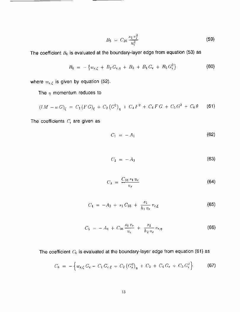
/35 = C2681¢'r2
The coefficient B6 is evaluated at the boundary-layer edge from equation (53) as
(59)
v, = -{,,¥._+ B2c.., + v3+ _,c._+ B5c_} (60)
where wc,¢ is given by equation (52).
The q momentum reduces to
(lM-wG)( = CI(FG)_ + C2(G°"),7 + C3F 2 + C4FG + CsG 2 + C60 (61)
The coefficients C, are given as
C1 = - A1 (62)
C2 = - A3 (63)
C3 - C34.sl u_ (64)'/3/.
C4 = -A2 + .sl C35 + 81 (65)-- Vr, _t_1 Vr
C5 A4 + C36 81 vr sl (66)= -- _ + _ Vr,T/ue h2 'ue
The coefficient C6 is evaluated at the boundary-layer edge from equation (61) as
13
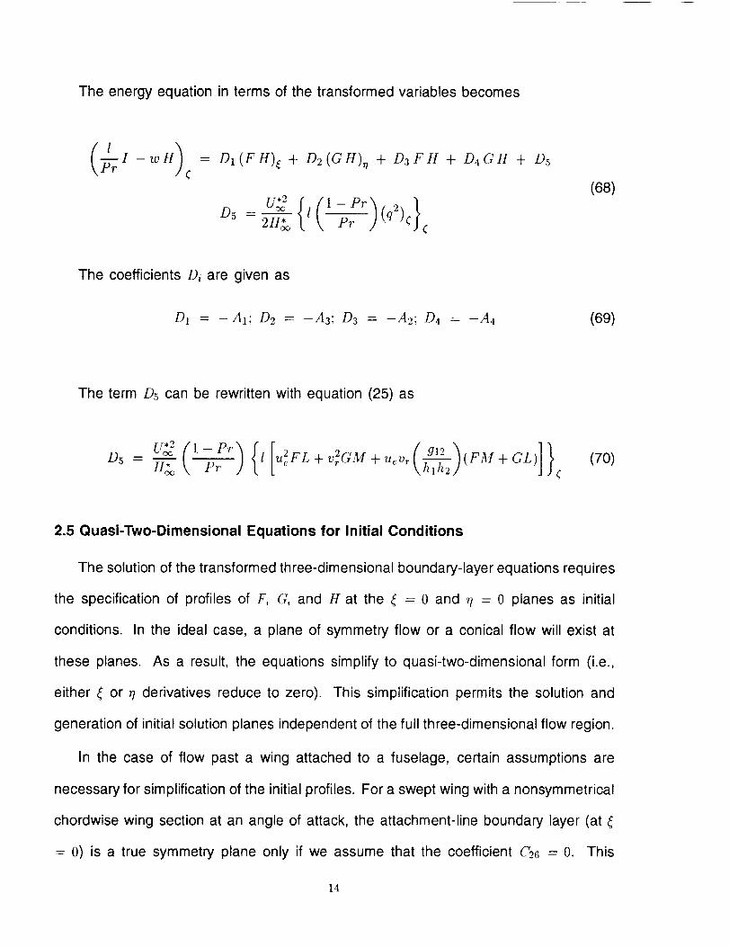
The energy equation in terms of the transformed variables becomes
(' )I -w H = D1 (FH)_ + D2 (GH), 7 + D3 F H + D4 G H + D5¢
_ U_ (1 - PrD5 2H_o {l Pr ) (q2)(}(
The coefficients D, are given as
(68)
D1 = -A1; D2 = -A3; D3 = -A2; D.I = -A4 (69)
The term D5 can be rewritten with equation (25) as
(,){[ ]}-Pr ( g,2 "_D5 - H_¢ fir l u_FL + v2_GM + ucv, k._j(FM + GL) ¢
(70)
2.5 Quasi-Two-Dimensional Equations for Initial Conditions
The solution of the transformed three-dimensional boundary-layer equations requires
the specification of profiles of F, G, and H at the ( -- 0 and q = 0 planes as initial
conditions. In the ideal case, a plane of symmetry flow or a conical flow will exist at
these planes. As a result, the equations simplify to quasi-two-dimensional form (i.e.,
either ,_ or q derivatives reduce to zero). This simplification permits the solution and
generation of initial solution planes independent of the full three-dimensional flow region.
In the case of flow past a wing attached to a fuselage, certain assumptions are
necessary for simplification of the initial profiles. For a swept wing with a nonsymmetrical
chordwise wing section at an angle of attack, the attachment-line boundary layer (at ,_
= O) is a true symmetry plane only if we assume that the coefficient C26 = 0. This
14

assumption is reasonable if the curvature of the attachment line is not significant. A
more drastic assumption is necessary for the q = 0 plane. We restrict the calculation
to a certain region on the wing, where the boundary-layer assumptions are valid. At
the q = 0 boundary, we assume that the q gradients of the flow variables are equal to
zero. However, we permit variation of the metric terms as well as the boundary-layer
edge quantities in both the ( and q directions. With this assumption, the equations
again reduce to quasi-two-dimensional form. This assumption is a more general version
of the conical flow assumption and is termed as the locally infinite, swept-wing (LISW)
assumption. The profiles at the ,_ = 0, 77= 0 location are generated by assuming that
the attachment line is infinite swept locally as well.
The equations that are valid for an LISW flow are obtained by setting the coefficients
A3 (hence, B2, C2, and 132)to zero. In the finite-differencing scheme, the q-direction dif-
ferencing coefficients are also set to zero. To obtain smooth solutions near this boundary,
the full three-dimensional solution is relaxed to the LISW solution by incorporating a fac-
tor _ = _(q) to be applied to these coefficients for a few planes adjacent to the r/ = 0
plane. A value of _ = 0 gives the LISW solution, whereas a value of _ = 1 gives the
full three-dimensional solution. A similar assumption of LISW flow is used at the 7-/=
T/m,x boundary as well.
The quasi-two-dimensional equations that are valid for an attachment line are more
involved because the ( momentum equation becomes singular at ( = 0 by substituting
u = 0. The gradient Ou/#( is finite, however. The effect of the strong inviscid flow
acceleration fe = o%e/0( on the attachment-line boundary layer is characterized by taking
the ,_ derivative of the ( momentum equation. The new definitions for the transformed
15

normal coordinate and normal velocity are
f d_Pe/_e hi
o
(71)
(72)
With these special transformations, the transformed equations are in the same form as
before (equations (46), (53), (61), and (68)) except that the following coefficients are
changed:
A1 = 0 (73)
A2 = - 1 (74)
hi Vr
A3 -- h2 f_ (75)
h, { CvT'_ (76)A4 - C13¢ C13 h2feJ,y
¢ = Jp,.,hlL (77)
B3 = 2 (78)
B 4 = hl Vr fe41 -- A4 4- C25 hiv____L (79)h2f_ L
2hl Vr
B5 : C26,x f_ (80)
16
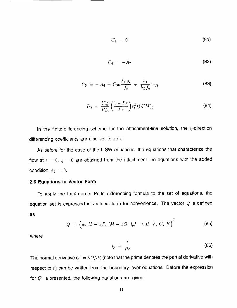
c3 = o (81)
C4 = -A2 (82)
hi vT hi (83)C5 = -A4 + C36_ + h2f_vr'_/
U_ (1-Pr) 2(lGM) ¢ (84)D5 H_ ° Pr Vr
In the finite-differencing scheme for the attachment-line solution, the (-direction
differencing coefficients are also set to zero.
As before for the case of the LISW equations, the equations that characterize the
flow at ( = 0, 7/ = 0 are obtained from the attachment-line equations with the added
condition .43 = 0.
2.6 Equations in Vector Form
To apply the fourth-order Pade differencing formula to the set of equations, the
equation set is expressed in vectorial form for convenience. The vector Q is defined
as
where
(86)
The normal derivative Q' = OQ/OC (note that the prime denotes the partial derivative with
respect to C) can be written from the boundary-layer equations. Before the expression
for Q' is presented, the following equations are given.
17

The density ratio 8 can be written from equation (24) in terms of the elements of Q as
0 = ElF 2 + E2FG + E3G 2 +E4H
X2 2 X2E1 - ue; E2 = - 2 -- ue vr cos /3
3/3 X3
X2 2. E4 X]E 3 -- Vr ; = --X3 X3
"y-i 2X1 = i + ---_-_I_o; X2 = X1 - i; X3 = HeXI - X2 q_
z
(87)
The viscosity ratio I can be written from equation (33) as
The normal derivatives l' and 0' can be derived in the form
(88)
0' = 2EIFL +E2(FM+GL) +2E3GM + E4I (89)
i, = 10.___'{ 1 t } (90)V'_ 2v"-0 (1 + T.IT,)
The QI' element is obtained from equation (46). The Q2' element is obtained by
substituting for 0 from equation (87) into equation (53).
Q_ = B1 (F2)_ + B2(FG). + /_3F 2 + B4FG + /_5C 2 -4- /_6H
/_3 - B3 + E1 B6; _4 = B4 + E2 B6; /_5 = B5 + E3 B6; B6 = B6 E4
(91)
The element Q3' is similarly obtained as
Q_ = C1 (FG), + C2 (a2), 7 + C'%.3F 2 + C.4FC + C.s G2 + C.6H
C'3 = C3 -t- E1C6; C'4 = C4 -4- E2C6; C5 = C5 -4- E3C6; C'6 = C6E4
(92)
18
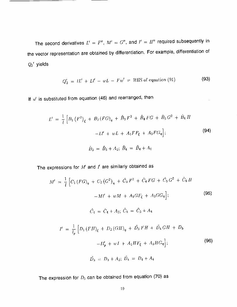
The second derivatives L' = F", M' = G', and I' = H" required subsequently in
the vector representation are obtained by differentiation. For example, differentiation of
Q2' yields
(2'2 = 1L' + LI' -wL- Fw' = RHSofequation(91) (93)
If _ is substituted from equation (46) and rearranged, then
LI 1= 7 [ ul (F2)(
+ B2 (FG), 7 + [?3 F2 + [_4 FG + [Y5 G 2 + [_6 H
-L# + wL + A1FF( + A3FG,_];(94)
B3 = /_a+A2; B4 = /_4+A4
The expressions for ,,t# and /' are similarly obtained as
M' = _1 [CI(FG), 7 + C2(G2),1 + Ca F2 + 04FG + CsG 2 + C6H1
-Ml' + wM + A1GF( + AaGG,7];(95)
C4 _ C4 qL A2; d_5 = C,5 qt_ A4
[i1
= 17 [D1 (FH)_ + D2(GH),_ + 15aFH + 154GH + D5
_.; + w1+ A,.r, + A..c..]; (96)
/53 = Da + A2; 1)4 = D4 + A4
The expression for D5 can be obtained from equation (70) as
19

D5
U .2 1 - PrAo - _ _, 2. A3 = AOUeVrCOS t_tt* Pr , A1 = Aou_2; t2 = Aovr,
(97)
Note that ,_1 = A3 = 0 for the attachment-line equations. The final vector repre-
sentation is given as
<2
1L - wF
IM - wG
lpI -- wHF
G
H
(98)
I =
/ AIF4 + A2F + A3Gq + A4G~ '3'
BI(F2)( + B2(FG). + B3F 2 + B4FG + B5G" + t_6H
CI(FG)(+C2(G 2) +¢3F 2+04Fc+C,5c 2+06H
DI(FH)( + D2(GH)_ + D3FH + D4GH + .D5L
31
I
(99)
AlL( + A2L + A3M, I + A4M "_
2BI(FL)( + B2(FM + GL)o + 2133FL + 1_4(F3,I + GL) + 2135G'M + BG[
C,(FM + GL)_ + 2C2(GM), 7 + 2('3PL + (-;4(PM + GL) + 2CsGM + ('GI
D,(FI + fIL)( + D2(GI + HM), 1 + D3(FI + HL) + D4(G[ + [Jill) + Dr5
L' (equation (94))
M' (equation (95))
I' (equation (96))
(loo)
2O
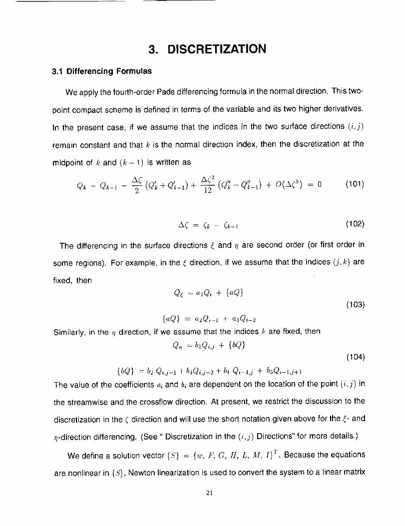
3. DISCRETIZATION
3.1 Differencing Formulas
We apply the fourth-order Pade differencing formula in the normal direction. This two-
point compact scheme is defined in terms of the variable and its two higher derivatives.
In the present case, if we assume that the indices in the two surface directions (i,j)
remain constant and that k is the normal direction index, then the discretization at the
midpoint of k and (k- 1) is written as
Qk - Qk-; A(_2 (Q_ + Q_--1) + _A_2 (Q_ - Qk-1)" + O(A_ 5) = 0 (101)
(102)
The differencing in the surface directions ( and q are second order (or first order in
some regions). For example, in the ,_ direction, if we assume that the indices (j, k) are
fixed, then
Q( = alQi + {aQ}
{_Q} = a2Qi-1 + a3Q,_2
Similarly, in the q direction, if we assume that the indices k are fixed, then
@1 = blQi,j + {bQ}
(103)
(104)
{bQ} = b2 Qi,j-1 + b3Qi,j-'2. + b4 Qi-l,j -F bsQi-l,j+1
The value of the coefficients ai and b, are dependent on the location of the point (i,j) in
the streamwise and the crossflow direction. At present, we restrict the discussion to the
discretization in the ( direction and will use the short notation given above for the (- and
q-direction differencing. (See " Discretization in the (i,j) Directions" for more details.)
We define a solution vector {5'} = {w, F, C, H, L, M, I} T. Because the equations
are nonlinear in {S}, Newton linearization is used to convert the system to a linear matrix
21

inversion problem. If superscript n denotes the current iteration stage, let us define {55'}
as
{5S} = S n-s n-] (105)
A linear system is now set up to solve for {5S} in terms of the solution at iteration level
n - 1. For example, a term that involves (F,,)2 is written as
(F") 2 = (F n-' +5F)2_ (F'_-')2+2F '_-' 5F (106)
In what follows, the superscript n - 1 is dropped and is taken to imply the known values
of {S} at iteration n- 1.
are given below:
A few examples of the linearized formulas with this notation
(Fn) 2 = F 2 -4- 2F 5F
F{ = F_ + alSF
F_ = F,_ + blSF (107)
F" F_ = FF_ + SF(alF + F_)
3.2 Linearized system at (i,I)
The system is explicit in ( and rt because of our choice of the finite-differencing
scheme and is implicit in the surface-normal direction. The linearized system is repre-
sented at location (i,j), which corresponds to the solution at iteration level n as
["" at_t,m b_m'"] {5S/_} = {r_} (108)
where a k and bk_,m _,mare elements of the (7 x 7) blocks in the diagonal and superdiagonal
locations of the linearized block bidiagonal system. The superscript k denotes that the
22
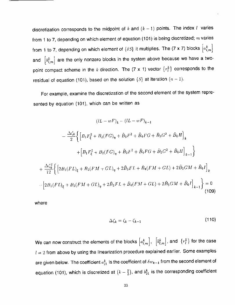
discretization corresponds to the midpoint of k and (k - t) points. The index I varies
from 1 to 7, depending on which element of equation (101) is being discretized; m varies
from 1 to 7, depending on which element of {55} it multiplies. The (7 x 7) blocks z,m
bk ] are the only nonzero blocks in the system above because we have a two-and t,m
point compact scheme in the k direction. The (7 x 1) vector {r_} corresponds to the
residual of equation (101), based on the solution {S} at iteration (n- 11.
For example, examine the discretization of the second element of the system repre-
sented by equation (101), which can be written as
(IL - wF)k - (IL- wP)k_ 1
2 k
-[2BI(FL)( + B2(F,_I + GL)q + 2#3FL + [34(FJ'il + GL) + 2#5G_I +/Y6/] k-1 } = 0
(109/
where
A(k = (k - (k-1 (110)
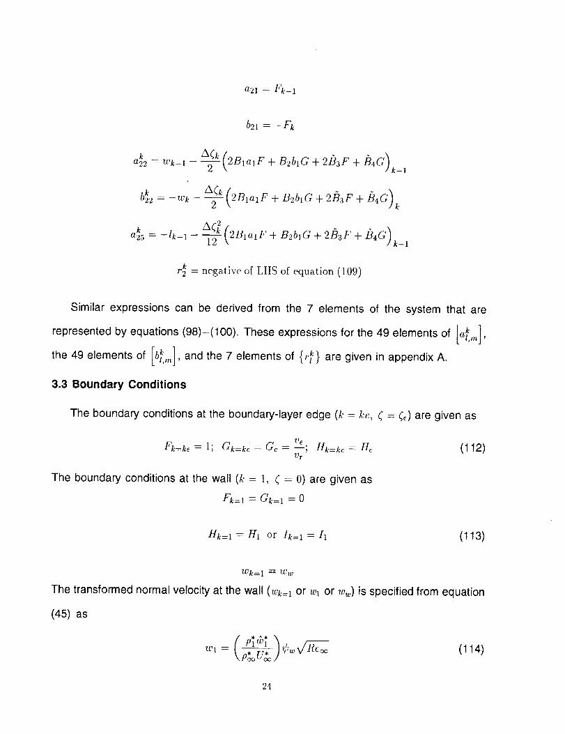
[a' I [bk ] and {rt k} for thecaseWe can now construct the elements of the blocks z,= , t,= ,
l = 2 from above by using the linearization procedure explained earlier. Some examples
are given below. The coefficient a_l is the coefficient of 5wk_l from the second element of
equation (101), which is discretized at (k- ½1, and b_l is the corresponding coefficient
23
a21 = Fk_ 1
b21 =--Fk
ak2 = Wk-l ----AG
2 /k-1
bk2 =--wk- --ACk
(2_lalr 4- B2blG 4- _b3r 4- h4G)2 \ ,'k
ak25 = --Ik-1 -- (2BlalF + B2blG 4- 2i)3F + .B4G'_12 \ / _-1
r2k = negative of LtIS of equation (109)
Similar expressions can be derived from the 7 elements of the system that are
a krepresented by equations (98)-(100). These expressions for the 49 elements of [ l,m],L J
[bk ] and the 7 elements of {r_} are given in appendix A.the 49 elements of t,,,, ,
3.3 Boundary Conditions
The boundary conditions at the boundary-layer edge (k = k,, ¢ = Ce) are given as
Fk=k_ = 1; Gk=k_ = Ge = --;v_ Hk=k_ = H_ (112)Vr
The boundary conditions at the wall (k = 1, ( = 0) are given as
fk=l = Gk=l = 0
Hk=l = H1 or lk= 1 -----11 (113)
Wk= 1 = W w
The transformed normal velocity at the wall (wk=l or w, or Ww) is specified from equation
(45) as
24
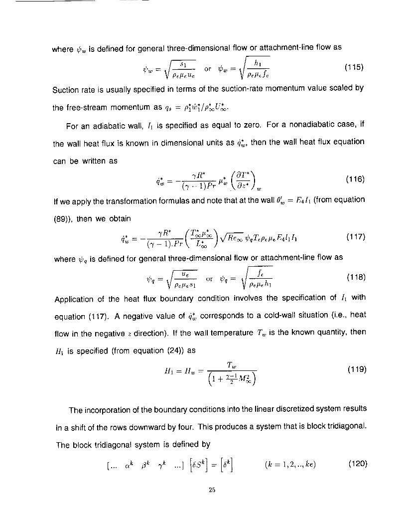
where _'w is defined for general three-dimensional flow or attachment-line flow as
i Sl i hithw = or _bw= (115)
pe#_ ue Pcffe f e
Suction rate is usually specified in terms of the suction-rate momentum value scaled by
the free-stream momentum as q, = plwl/poouoo.
For an adiabatic wall, [1 is specified as equal to zero. For a nonadiabatic case, if
the wall heat flux is known in dimensional units as _,_, then the wall heat flux equation
can be written as
.. ,.,/R* . (OT*'_ (116)qw = (_/ZSpr#W \Oz*Jw
If we apply the transformation formulas and note that at the wall O" = E411 (from equation
(89)), then we obtain
., 7R* (T*It*)_ ¢qTepetteE411[ 'q_ = ('7- 1).Pr L*
where _q is defined for general three-dimensional flow or attachment-line flow as
(117)
__p u_ _/ f_ (118)or Cq_q eZ81 fle#e hl
Application of the heat flux boundary condition involves the specification of Ix with
equation (117). A negative value of ,_, corresponds to a cold-wall situation (i.e., heat
flow in the negative z direction). If the wall temperature T,,, is the known quantity, then
HI is specified (from equation (24)) as
H1 = Hw =T_
1 _-1 M2 "_+2 ocj
(119)
The incorporation of the boundary conditions into the linear discretized system results
in a shift of the rows downward by four. This produces a system that is block tridiagonal.
The block tridiagonal system is defined by
[...
25
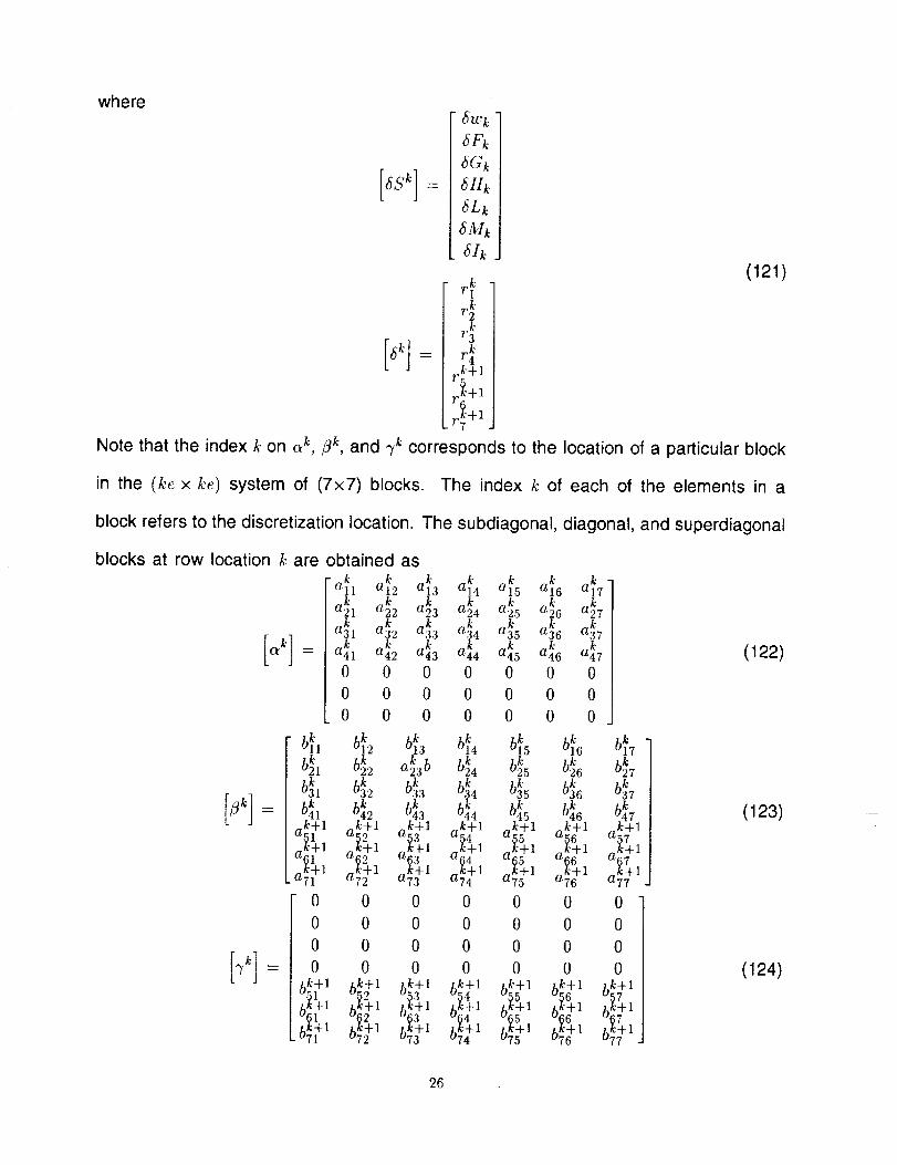
where
6S k]
"&wk7
5Gk= 611k
6Lk ]
+M++l_a[k J
(121)r_
r_[+,]=
iiiNote that the index k on a k, ilk, and @ corresponds to the location of a particular block
in the (ke x ke) system of (7x7) blocks. The index k of each of the elements in a
block refers to the discretization location. The subdiagonal, diagonal, and superdiagonal
blocks at row location k are obtained as
a3kl
a4kl
0
0
0
blkl blk2
bkl bk2
q, Gbkl bk2
akt 1
a_+l
.}}10
0
0
0
bk+_
,,1+.+a,++'+,+4a,++a,+++ '+++4a+++a+++a2k2 a23
a+2 a+3 a_4 a3k5 ak6
a4k2 a4k3 a4k4 a4k5 a4k+
0 0 0 0 0
0 0 0 0
0 0 0 0
+'1+++'h +',++a+3b bk24 b#5
bk33 bk4 bk35
¢,3 G +4ak+1 ak+l akS: 1 a k+l
a_+ 1 a_: 1 ak6+41 a_t 1
0 0 0 0
0 0 0 0
0 0 0 0
0 0 0 0
bblff: :lffll :..,.,}t._-:, bblff:
a_17a_7
ak7
ak47
0
0 0
0 0
_k46ak+l
a_+l
0
0
0
0
bk+_
b_7b_7G
_k+l
:_-1
a7 +1
0
0
0
0
bk¢ 1
b_7q-1
(122)
(123)
(124)
26
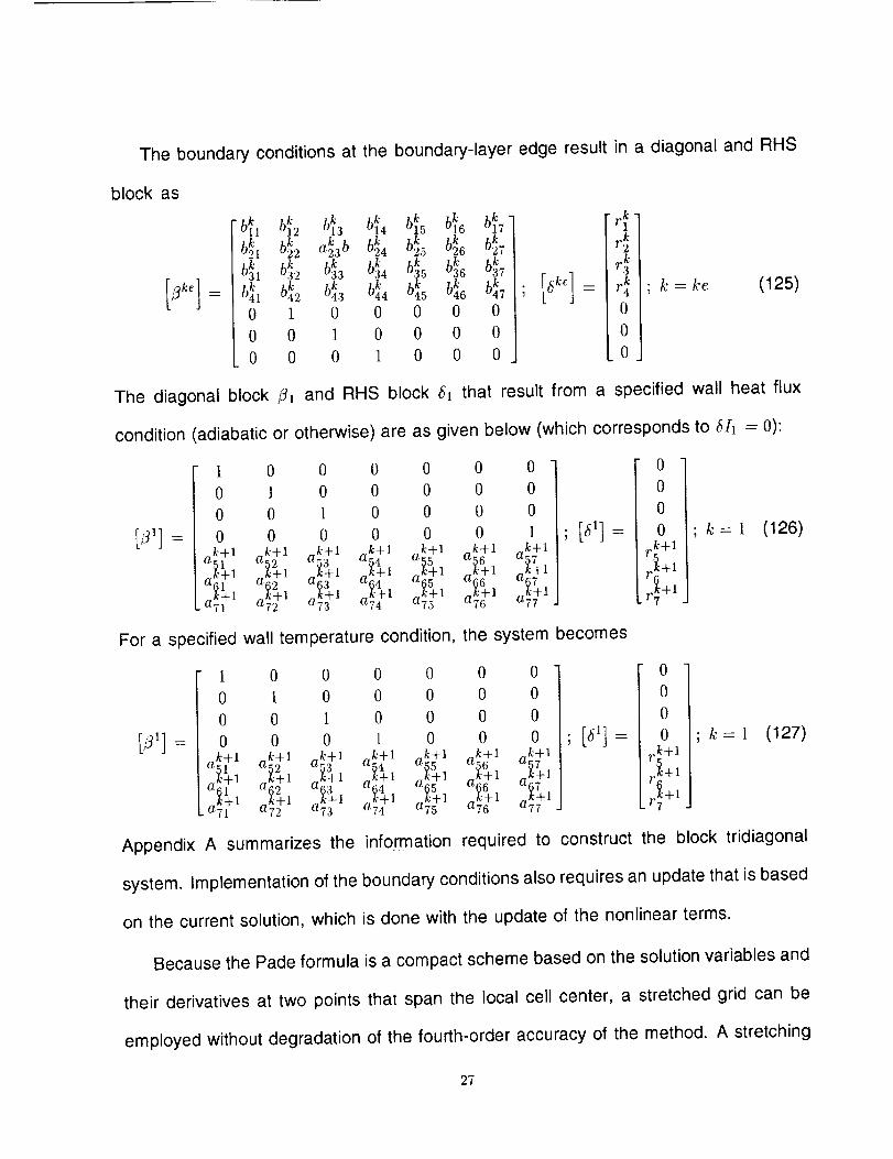
The boundary conditions at the boundary-layer edge result in a diagonal and RHS
block as
0 1 0 0 0 0 0
0 0 1 0 0 0 0
0 0 0 1 0 0 0
4
4r4k ; k = ke
0
0
(125)
The diagonal block _'1 and RHS block 51 that result from a specified wall heat flux
condition (adiabatic or otherwise) are as given below (which corresponds to 5[1 = 0):
1 0 0 0 0 0 0
0 1 0 0 0 0 0
0 0 l 0 0 0 0
0 0 0 0 0 0 1
aktl _k+l k+l k+l k+l ok+l k+l
a_? 1
For a specified wall temperature condition, the system becomes
1 0 0 0 0 0 0
0 1 0 0 0 0 0
0 0 1 0 0 0 0
0 0 0 1 0 0 0
aktl _k+l ak_, _k+l ak_l ak_l _k+l•"4 a_+l
0
0
0
0
rk+l
r_-+l
F_ +1
; k = 1 (126)
0
0
0
0
rk+l
ir_+ 1
L4+1
;k=l (127)
Appendix A summarizes the information required to construct the block tridiagonal
system. Implementation of the boundary conditions also requires an update that is based
on the current solution, which is done with the update of the nonlinear terms.
Because the Pade formula is a compact scheme based on the solution variables and
their derivatives at two points that span the local cell center, a stretched grid can be
employed without degradation of the fourth-order accuracy of the method. A stretching
27

constant k, is defined to exponentially stretch the grid in the ( direction as
(128)
3.4 Discretization in the (i,j) Directions
In the fully three-dimensional region (away from the attachment line and side bound-
aries, j = 1 or j = ny]im), the differencing in the surface directions ( and 7j is done to
second-order accuracy. In accordance with the parabolic nature of the equations, the
derivative is obtained by the three-point upwind-differenced formula
(fe)_,j = a_f,,j + a2f,-_,j + a3fi-2,j
9 9 '3
al = (A(;- zx(,_,)lA; = -A ;la; = zx _,lA (129)
A = ,--._iA_i-l(A_i 4- A_i-1); A_i = _i,j - _i-l,j; A_i-1 = _i-l,j - _i-2,j
When i = 2, the first-order formula with just two points is used, which results in the
coefficients
al = l/A(2 = 1/(,_2 -,_1); a2 = -al; a3 = 0 (130)
A function _i is used to blend the first-order and second-order formulas in a small number
of marching steps. The short notation {aF} used in equation (103) can thus be expanded
in terms of the coefficients given above. At ,_ = 0, the attachment-line equations do not
contain any 0/0( terms; this condition is incorporated into the solution scheme by setting
up a flag set to zero for the attachment-line solution and to unity for i > 1.
The q differencing is accomplished with a combination of two schemes. For situations
where the profile G is positive at all normal grid-point locations, the standard left-pointing
three-point second-order scheme (which we refer to as the L scheme) is used. When
28
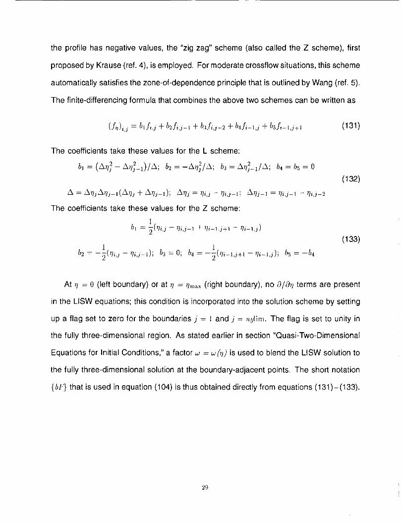
the profile has negative values, the "zig zag" scheme (also called the Z scheme), first
proposed by Krause (ref. 4), is employed. For moderate crossflow situations, this scheme
automatically satisfies the zone-of-dependence principle that is outlined by Wang (ref. 5).
The finite-differencing formula that combines the above two schemes can be written as
(fTI)i,j = blfi,j + b2fi,j-1 + b3fi,j-2 -k b4fi-l,j + b5fi-l,j+l (131)
The coefficients take these values for the L scheme:
bl = (_q_ - A,__,)/_; b2 = -Aq_/A; b3 = _q__l/_; b4 = b5 = 0
A = ,2._rl/A.qj_l('2._q. / + Arlj_l); /kq./ = qi,j - Ill,j-l; _--_r]j-1 = 7]i,j-1 - Tli,j-2
The coefficients take these values for the Z scheme:
]bl = _(71ij - qi,j-a + _ti-lj+a - T/i_a,j)
1 1b2 =--_(_,._-qij-1); b3 =0; b4 =--_(qi-ij+_-qi-_,j); b5 =-b4
(132)
(133)
At q -- 0 (left boundary) or at q -- T/re,× (right boundary), no O/Oq terms are present
in the LISW equations; this condition is incorporated into the solution scheme by setting
up a flag set to zero for the boundaries j = ! and j = nylim. The flag is set to unity in
the fully three-dimensional region. As stated earlier in section "Quasi-Two-Dimensional
Equations for Initial Conditions," a factor _ = _ (_) is used to blend the LISW solution to
the fully three-dimensional solution at the boundary-adjacent points. The short notation
{b£} that is used in equation (104) is thus obtained directly from equations (131)-(133).
29

4. INVISCID INTERFACE
The three-dimensional boundary-layer solution procedure is based on the specifica-
tion of the edge quantities u_, v_, and T_ on a surface grid defined in the coordinate
directions ( and q. In addition, the computation of the edge density p_ requires the spec-
ification of the inviscid pressure P or the pressure coefficient Cp (for flows that involve
a shock between the free stream and the attachment line). In the general case, for a
nonorthogonal boundary-layer grid, the metric quantities h_, h2, and g12are also assumed
to be given. Further, the edge value of viscosity t_ is computed from T_ with the Suther-
land formula (equation (33)). The above quantities are referenced to the free-stream
quantities (U_o, P_o, and T_) and the reference length L_o.
If we assume that a negligible interaction occurs between the viscous and inviscid
regions, the edge conditions can be obtained by solving the three-dimensional Euler
equations on a sufficiently fine mesh. In some cases such as low-speed flow, a
potential panel code may be substituted in place of the Euler solver, after which an
interface procedure is necessary to process the inviscid results to express them in the
form required by the boundary-layer code. Specifically, this procedure involves (a) the
accurate location of the inviscid attachment line, (b) the generation of the boundary-layer
grid which originates from the attachment line on the upper or lower surface, (c) the
calculation of the edge velocities in surface grid-oriented directions, and (d) the output
of quantities in the required form for the boundary-layer code.
Two approaches are used to calculate the edge velocities (u_, v_) and edge tem-
perature T_. The first approach is to interpolate the inviscid pressure distribution onto
the boundary-layer grid and then calculate the edge velocities and temperature by solv-
ing the limiting equations of the boundary-layer equations at the boundary-layer edge.
3O

These limiting equations (henceforth called the BL-EDGE equations) are hyperbolic and
can be solved with a marching method that is analogous to the boundary-layer solution
procedure. The source term in these equations is the pressure gradient in the two di-
rections ( and T/. The second method involves the interpolation of all the required edge
quantities from the inviscid grid to the boundary-layer grid.
The first procedure is, in principle, more consistent with the boundary-layer solution
method; however, the solution of the BL-EDGE equations may be slightly different from
the solution of the Euler equations. This mismatch in the edge quantities from the two
solutions is attributed to (a) the terms dropped in the BL-EDGE equations, based on the
boundary-layer assumption, and (b) variations in the finite-differencing schemes. In one
case, we have the edge velocities computed from the Euler equations, whereas, in the
other case, the edge velocities are computed from the limiting boundary-layer equations,
based on the Euler pressure gradient. The BL-EDGE equations also assume that the
edge total enthalpy is a constant, which is not necessarily true for the Euler solution.
Note also that accurate enforcement of the condition _3P/c3x = 0 at the attachment line
is difficult from a coarse inviscid grid, which may necessitate that the interpolation near
the attachment line be linear rather than spline to ensure a negative pressure gradient
at the attachment line. The interface program includes an option to calculate the edge
conditions by either method.
4.1 Attachment-Line Relocation
After the surface pressure distribution is obtained from the inviscid calculation, the
initial location of the attachment line is obtained by scanning for a maximum pressure in
the vicinity of the leading edge of the wing. However, note that the true attachment-point
location may be located within a bandwidth of one grid point on either side. The true
31
location of the attachment point is where the surface velocity in the direction normal to
the attachment line is equal to zero.
In this procedure, the Cartesian velocity components of the Euler solution are con-
verted to surface-oriented velocities that correspond to a boundary-layer surface grid
generated from the initial attachment-line location. This velocity conversion is based on
equations (13)-(17). In general, the component u_ at the initial attachment point will be
nonzero. This point is then relocated in the positive or negative direction, depending on
the value and sign of u_ and the local estimated value of 0,_/0s1. For example, for the
upper surface at an angle of attack, a relocation in the positive direction means that the
point is moved to include more of the lower surface; this is done when u_ has a positive
value. After the points are relocated with this logic, a new boundary-layer surface grid
is generated from these attachment-line locations. New values of velocity components
are obtained by interpolation. This procedure is repeated until the value of u_ at each at-
tachment point is less than a specified tolerance value. A parameter _,t is used to relax
the relocation displacement and to ensure that the iterated locations remain within the
grid-point bandwidth mentioned above. Upon convergence, the pressure is interpolated
with a spline routine from the inviscid grid to the final boundary-layer grid.
4.2 Edge Values by Interpolation
Edge velocities and temperature are obtained by spline interpolation. For a fine
inviscid grid, this method usually produces smooth edge conditions comparable to the
solution from the BL-EDGE equations.
4.3 Edge Values from BL-EDGE Equations
The three-dimensional boundary-layer equations (eqs. (19) and (20)), when applied
32
at the edge of the boundary layer, result in the BL-EDGE equations and are given as
ue Ve . ( hlh_ h1912 ) 1--hl tte,z -t- _ tte,y nt- C24 lz;_ -t- C25 uct¥ -[- 026v 2 = Cf3_ Px + --C_3 PY _/p_M_ (134)
ue ve ('h2g,2 Pz h_h2 _ 1 (135)'tPe M_
Further, H_ is assumed to be constant. With P specified from the inviscid solution, the
following equation provides closure for this hyperbolic set of equations:
Te=Hc(I-t-'_M_) "7-1_. M_q_(136)
The solution to the above system is obtained with a discretization that is identical to the
full three-dimensional boundary-layer equations in the two surface directions. With the
abbreviated notations for the _ and r/directions, a discretization with Newton linearization
yields the system
[ ' (2alue+{aue}+blvc____-[l(alt'e + {ave})
where
+ {b,,o}) ]7_2(allte_-[- 2blt¥ -[- {bye})
nl 0£ o 2 oy (137)
The terms marked by an underline apply to the three-dimensional region only. These
terms are set to zero per the LlSW condition at j = I and j = ny. Note that the Py terms
are retained for LlSW, however.
The solution is obtained by inversion of the system, which is followed by an iterative
update for nonlinear terms.
33
5. BL3D EXAMPLE CASES
Two test cases are presented here. The first test case is that of a moderately swept
(A = 33°) tapered wing in subsonic flow. The streamwise cross sections of this wing
correspond to NACA 0012; however, for generality, calculations of metrics and other
parameters are done with the assumption that the wing is defined in terms of discrete
coordinates. The second test case is a highly swept (._ = 70°) wing in supersonic
flow, similar in planform to that of the F16XL aircraft, with cross sections defined in
discrete coordinates. For both cases, the inviscid results are obtained by solving the
Euler equations. The computer code CFL3D (ref. 6) is used for this purpose, with the
viscous terms set to zero for the Euter calculation. An interface routine processes the
results and feeds the resulting edge conditions to BL3D. For validation (case 1 only),
the results obtained from BL3D are compared with the results from the thin-layer Navier-
Stokes code, which is also obtained with CFL3D. For the supersonic wing case, we
present comparisons of the BL3D results with the solution from a conical swept wing
boundary-layer code developed by Kaups and Cebeci (ref. 3). In addition, runs are
made with a uniform suction distribution (case 1 only). These results are also compared
with the corresponding Navier-Stokes solution.
5.1 Geometry and Conditions for Case 1
The planform of this wing is a trapezoid for which the root chord is 1 ft and the
leading-edge sweep is constant at 32.73 °. The wing has a span of 2 ft and the trailing-
edge sweep is constant at 18.88 °, which results in a tip chord of 0.398 ft. The tip-section
leading edge is at x'* = 1.286 ft and the tip-section trailing edge is at x'* -- 1.68.1 ft.
The streamwise cross section of the wing corresponds to the NACA 0012 section. The
free-stream conditions are Moo = 0.5, ,_ = 2°, P* = 2116 psf, and Y_o= 520°R. The wing
34

is assumed to be symmetrical about the root chord plane.
5.2 Euler Solution for Case 1
The surface distribution used in the Euler grid consists of constant percent chord lines
and constant percent span lines. In the spanwise direction, the grid has 41 points on the
wing surface, which corresponds to a span distance of 0.05 ft between grid lines. In the
chordwise wraparound direction, the grid has 257 points, and in the wall-normal direction
the grid has 49 points that are stretched exponentially. The grid is further extended into
the wake region and off the tip of the wing. The Euler computation is done with the code
CFL3D. The results from the calculation are obtained at the centers of the grid cells;
thus, 40 cell centers exist in the spanwise direction. Let us denote these locations by
the symbol j(INV). To avoid the region very close to the symmetry plane and the wingtip,
we restrict our analysis to the region 7 < j(INV) < 35, which corresponds to 0.325 < gr. <
1.725. The middle location of this region is at j(INV) = 21, which corresponds to y'* = 1.025.
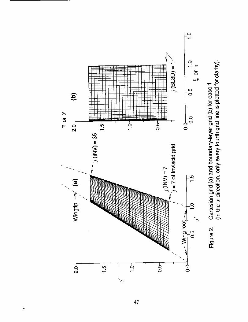
Figure 2(a) shows the surface distribution of the Euler grid-cell center points (note
that only every fourth point is plotted in the chordwise direction for clarity). Figure 2(b)
shows the corresponding boundary-layer grid on the upper surface. The boundary-layer
grid originates from the attachment line, and the z-coordinate is measured in terms of
the surface arc length, which is normalized by a length such as the local chord length or,
in the present case, by the maximum arc length. The spanwise coordinate y is defined
as the local span distance from the symmetry plane.
The inviscid results used in the interface routine are the three Cartesian components
of the velocity on the wing surface, the inviscid wall density, and the temperature.
The pressure coefficient on the surface can be calculated from the above. Alternately,
the pressure coefficient can be specified, and the edge temperature can be calculated
35
(assuming that the edge density is given). Figure 3 shows the variation of the pressure
coefficient obtained from the Euler solution at three span locations where j(INV) = 7, 21,
and 35. Note that the effect of the taper is to create a favorable pressure gradient in
the spanwise direction.
5.3 Euler-BL3D Interface for Case 1
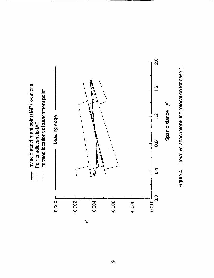
The details of the procedure for relocating the inviscid attachment line are presented
in Figures 4-7. Figure 4 shows a plot of the iterated attachment-line locations. This plot
is in terms of (fl, _) of these surface points and corresponds to a view from upstream of
the wing leading edge (not to scale). The initial attachment-line location that corresponds
to the peak in the pressure coefficient near the leading edge is shown in solid symbols.
The inviscid grid points on the upper and lower sides of this line are shown as dashed
lines. These lines bound the uncertainty on the true attachment-line location because of
the coarseness of the inviscid grid. Also shown in Figure 4 are the iterated locations of
the attachment line. As explained in "Attachment-Line Relocation," the iteration is based
on a relocation strategy such that the local inviscid velocity vector is exactly tangential
to the attachment line. Note that the line that joins the final attachment-line locations is
much smoother than the original line.
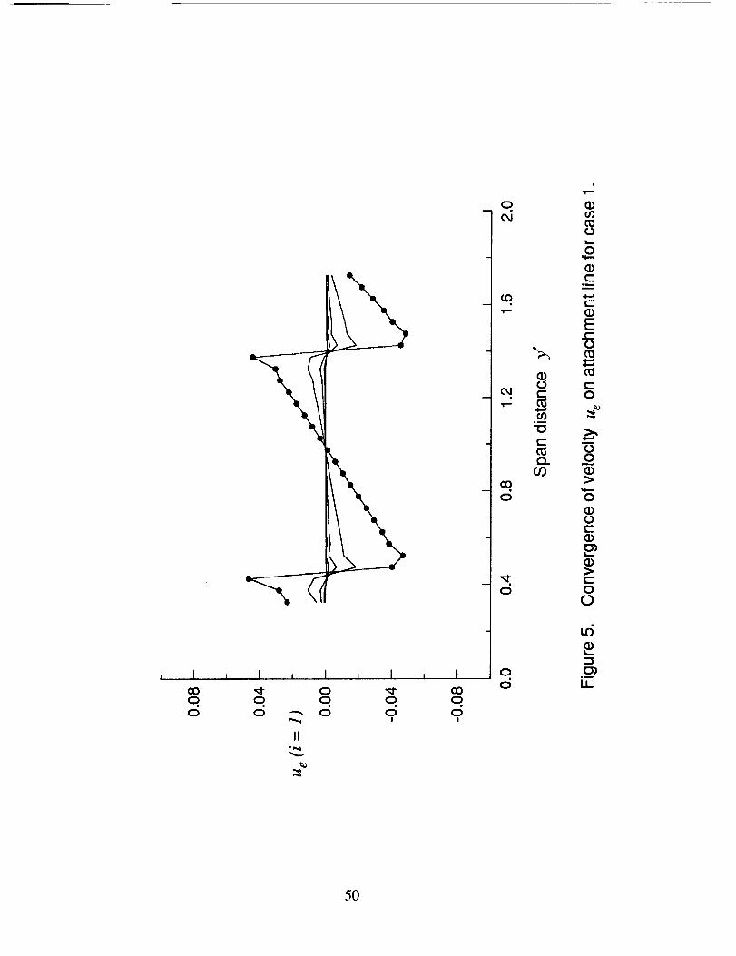
Figure 5 shows the velocity ue interpolated at the attachment-line location that
corresponds to successive iterations. Note that the initial values of u_ are relatively
high (_+0.04) and that the objective of driving _t_ to near zero (< 0.0001) is achieved
in seven iterations. Figure 6 shows the corresponding variations of the velocity _,_on
the attachment line. Here again, the final v_ variation is smooth. Figure 7 shows the
resulting variation of Cp on the attachment line.
The boundary-layer surface grid is generated from the attachment line on the upper
36

or lower side. In the present case, 40 points are generated in the chordwise direction
between the attachment line and the local 5 percent chord location. Beyond this point,
the boundary-layer grid coincides with the inviscid grid, and no interpolation is required.
The stretching of the surface distribution near the attachment line is done so that the grid
blends smoothly with the inviscid grid (at the 5 percent chord location in the present case).
After the generation of the surface grid, the inviscid pressure is interpolated to the
boundary-layer grid. The boundary-layer calculation is restricted to the region that is
bounded by the j(INV) = 7 and j(INV) = 35 spanwise locations. The regions outside
these limits are unsuitable; the locally infinite-swept wing assumption does not apply in
these regions because of the proximity of the flow to the symmetry plane or the wingtip.
The boundary-layer grid notation denoted by j(BL3D) is thus based on the left boundary
of j(INV) = 7. In other words, the j(BL3D) = 1 location is identical to the j(INV) = 7 location.
Figure 8 shows the chordwise variation of the interpolated Cp values on the boundary-
layer grid at three spanwise locations. The interpolation is accomplished with a spline
routine. In the present case, because the inviscid grid has good resolution near the
leading edge and the inviscid results are smooth in this region, no smoothing is required.
However, in the absence of the above, a smooth spline interpolation may be required.
In this event, the amount of smoothing and the resulting interpolated pressures must
be carefully monitored. If the streamwise pressure gradient at the attachment line is
not negative, a marching of the boundary-layer solution away from the attachment line
may not be possible. Spline and other higher order interpolation methods are likely to
introduce nonnegative pressure gradients at the attachment line. Hence, in some cases,
a locally linear interpolation may be required near the attachment line to ensure negative
pressure gradients.
All physical distances, such as the root chord length, are normalized by a reference
37

length L*. Further, the boundary-layer grid # (and _-) coordinate is defined as the local
chordwise arc length divided by the local maximum arc length up to the trailing edge. The
boundary-layer grid y- (and also T/-) coordinate is defined as the local spanwise distance.
With this definition, the metric quantities can be computed with equations (1)-(3). For
the present case, the variation of hi, h_, and g12 in the chordwise direction at the j(BL3D)
= 1 location is shown in Figure 9.
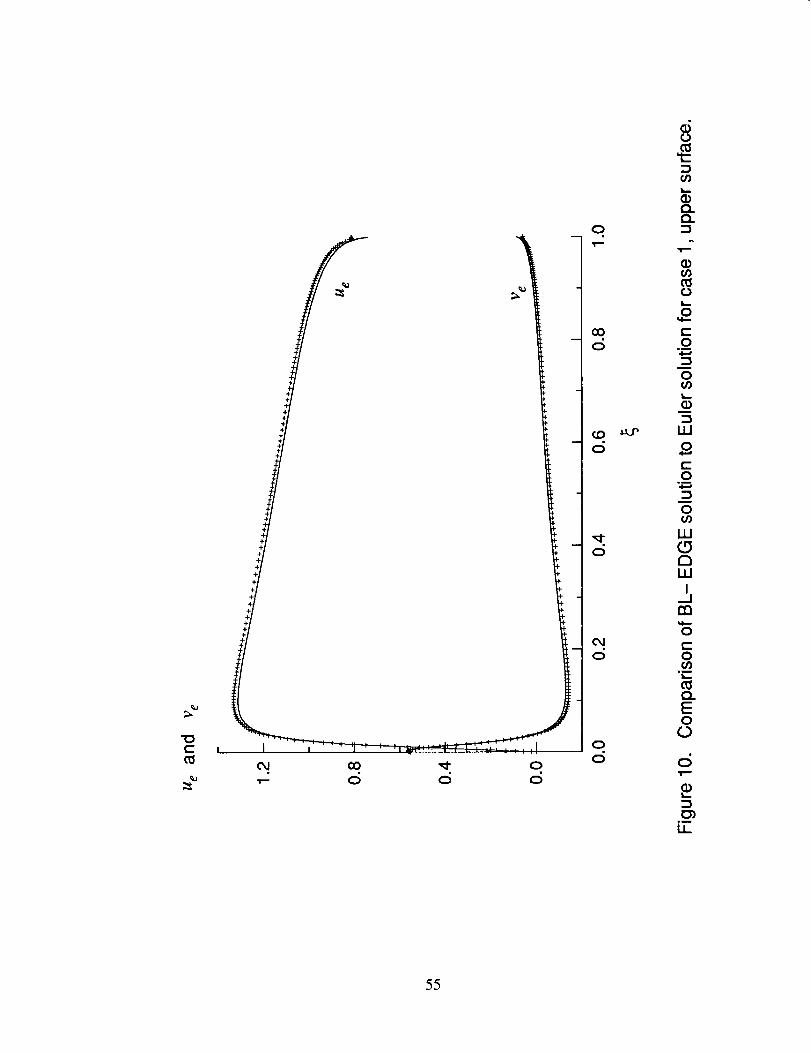
As explained in "Edge Values by Interpolation," the edge velocities can be obtained
by direct interpolation. In this method, the three Cartesian velocity components from
the inviscid solution are interpolated. Subsequently, the edge velocities in the z and y
directions are obtained by an inversion of the system given by equations (13)-(17). The
edge temperature is also interpolated to complete the interface to the BL3D program.
In the second method, the BL-EDGE equations are solved with the input pressure
distribution as outlined in "Edge Values from BL-EDGE Equations." Figure 10 shows a
comparison of the edge velocities obtained by either method at the j(BL3D) = 1 location.
Note that the two results agree well. Figure 11 shows contour plots of the edge velocity
ue on the upper surface of the wing that are obtained from the two methods. A slight
difference in the variation is caused by the fact that the BL-EDGE solution assumes
a locally swept-wing condition at j(BL3D) = 1 and j(BL3D) = 29. Another cause for
this difference is that the finite differencing used in the Euler solution is different from
that used in the BL-EDGE solution. However, for the present case, both results are
acceptable. Figure 12 shows the corresponding comparison of the edge velocity v_. The
edge temperature variations also compare well.
5.4 BL3D Solution for Case 1
The three-dimensional boundary-layer solution follows the sequence below:
38
(a) Input boundary-layer edge data. The input consists of the boundary-layer grid
dimensions (u=, ny); the coordinates (x, y); the metric quantities hi, h2 and g12; and
edge values u_, re, and T_. Further, if the streamline between the free stream and
the boundary-layer attachment line contains a shock (nonisentropic region), then the
input of Cp or P is required to calculate the edge density p_. Other inputs are the
free-stream conditions, the reference length, and other parameters that pertain to the
solution procedure.
(b) Setup of initial profiles. Solution profiles that correspond to the similarity solution
for a flat plate or wedge are used as initial profiles to start the locally infinite, swept
attachment-line solution at i = 1, j - 1 of the boundary-layer grid.
(c) Setup of edge coefficients. This setup is based on the edge conditions and
gradients. The coefficients A_, B_, C,, and D, are calculated.
(d) LISW solution. This solution is obtained at the two boundaries j = 1 and j = ny]im
by marching in the x direction. The terms that involve derivatives in the y direction are
set to zero for this case. Further, at i -- 1, the attachment-line equations are solved.
(e) Solution of the three-dimensional region. Given the initial plane solution and
the side boundary solution, the three-dimensional region can now be solved with the L
scheme or the Z scheme for the span derivatives. A switching from the L scheme to the
Z scheme occurs when the profile of G has a negative element.
Depending on the pressure distribution, the solution region can be restricted to (1,
nxlim), (1, nylim). After the convergence of the solution at each (i, 3) point, quantities
such as the boundary-layer thickness, the skin-friction coefficient, and the crossflow
Reynolds number are calculated.
39

5.5 BL3D Results for Case 1
Comparison of the BL3D solution is made with profiles that are obtained from the
solution of the NS equations with the code CFL3D. This code was run on a grid with the
same surface distribution as the Euler grid, but with 81 points in the wall-normal direction.
The grid stretching was designed to include about 30 to 40 points in the boundary layer
of the flow. The flow was assumed to have an abrupt transition to turbulence at the 25
percent location on the wing. This assumption ensures that the flow remains attached
and thereby avoids the numerical problems caused by the laminar separated regions.
The profile comparisons are restricted to locations upstream of the 25 percent chord
station. Because of the large amount of data, the comparison plots are presented for a
few locations in the flow that are representative of the entire flow solution.
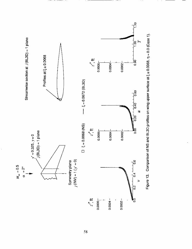
Figures 13-18 compare of the BL3D and NS profiles at the j(BL3D) = 1 plane.
We present comparisons at six locations in the chordwise direction. These locations
approximately correspond to chord locations of 1, 2, 3, 6, 12, and 23 percent. Shown
are the profiles of spanwise velocity v, chordwise velocity u, and temperature T. At
these locations, the spanwise velocity profile assumes different shapes with inflection and
reversal regions. The NS profiles are shown in open square symbols. The BL3D profiles
at this j location are the solution of the LISW equations. In spite of this assumption,
very good agreement is obtained until the 23 percent chord location. Note that the edge
velocities used as input for the BL3D computation are the interpolated values from the
inviscid code. The edge velocities that are computed from the NS solution are slightly
different than those from the Euler solution. This difference is the main contributor to
the lack of better agreement between the two solutions. Also, some differences are
attributable to the fact that the profiles are not compared at exactly the same location.
The temperature profiles at the 12 percent chord location and beyond are different
4O

presumably because the boundary-layer interaction becomes more significant in this
region. Furthermore, some differences near the attachment point are caused by the fact
that the attachment point from the NS solution is shifted slightly compared with the Euler
location. Overall, the agreement is satisfactory and validates the BL3D results.
The program also calculates the crossflow within the boundary layer relative to the
local edge streamline direction. In the present report, crossflow is defined as negative
when pointed toward the wing root. In Figure 19, we compare the streamwise velocity
profiles u8 at six representative locations with the corresponding NS profiles. Figure 20
shows the corresponding crossflow velocity profiles of v,. The crossflow that is predicted
by the BL3D code is slightly larger than the NS solution in the negative crossflow region.
The crossflow Reynolds number Rec£ is defined as
ReC_ p = Ue'maxOO'lPe (138)
* ,* and 8_.1 is thewhere V,,m,_×is the maximum absolute value of the crossflow velocity v_
normal distance at which the v_ profile decays to less than 10 percent of V*,m_,x (when
scanned from the edge down to the wall). This parameter has a strong correlation to
the growth of crossflow instabilities in a three-dimensional boundary layer. Figure 21
shows the variation of this parameter in the chord direction at the j(BL3D) = 1 location
compared with the NS solution.
Figures 22-30 present the profiles at the j(BL3D) = 15 location at the { = 1.025
spanwise station. The overall comparison is good, although in some locations differences
in profiles exist mainly because of the fact that the edge conditions from the NS and
Euler results are different.
Figure 31 shows the contours of the boundary-layer thickness and the skin-friction
coefficient in the x direction obtained from the BL3D calculation. The contours are smooth
41

and blend smoothly with the infinite swept-wing solutions at the j boundary locations.
Note that the flow is close to laminar separation as indicated by the near-zero values
of Cf,x at ,_ = 0.25.
Figure 32 shows the contours of the crossflow Reynolds number and the maximum
absolute percent crossflow on the upper surface. The values of RecF for this case are
under 100, and the maximum crossflow reaches a maximum of about 12 percent.
5.6 Results With Suction for Case 1
Solutions were obtained from the NS and BL3D solvers with boundary-layer suction.
A constant amount of suction q, (equal to 0.0005) was assumed. Figure 33 shows a
comparison of the resulting solution profiles at the j(BL3D) = 15 plane. The profiles with
no suction are also shown for comparison. Figure 34 shows the resulting Rec£ values;
a substantial reduction is produced in the crossflow with suction.
The attachment-line Reynolds number Re0 is defined as
V 'k i1_ '_
Ree = _,i=l m,i=lfle,i=l (139)#*,i=]
where e* is the momentum thickness. This parameter is important because of
attachment-line stability considerations. Figure 35 shows a comparison of the Re8 values
at the attachment line both with and without suction. The comparison with the values
obtained from the NS solution is satisfactory.
5.7 Geometry and Conditions for Case 2
Case 2 is the boundary-layer flow on a supersonic wing of 700 sweep at a free-
stream Mach number Moo of 1.6 and at an angle of attack of 0 °. The planform is similar
to the wing of the F16XL aircraft. The other input free-stream conditions correspond
42
to an altitude of 40,000 ft ( P% = 393.13 psf, Tgo = 390°R). The free-stream Reynolds
number is 3.06x 10⁶ per ft.
Figure 36 shows a top view of the Euler grid used in this case, with an inset showing
a chordwise section. The wing is assumed to be symmetric about the (x'*, z'*) plane at
the span station j(INV) = 1, which is at a distance of 27 in. from the fuselage axis. The
flow region of interest corresponds to the y'* range of 72.8 to 132.2 in.
5.8 Euler Solution and BL3D Interface for Case 2
The inviscid pressure distribution on the wing upper surface, obtained from the Euler
solution, is shown in Figure 37. Here, the streamwise distances are shown in terms
of x'* '* which corresponds to the chordwise distance from the local leading-edge-- .r LE ,
location. The variation of pressure coefficient and the wing cross section at the span
location j(INV) = 16 (90.2 in. from fuselage axis) is shown in Figure 38. Attached laminar
flow does not exist beyond a x'* _* distance of 3 ft; hence, the calculations reported-- .7:LE
here are for an x'* - xL£'* of less than 3 ft.
The interface program is essentially in the same form as case 1, except for minor
changes in reading in and manipulation of the Euler solution input. The boundary-layer
grid is specified as containing 40 points clustered within the 2 percent chordwise location.
The edge velocities and temperature are calculated either by direct interpolation or by
solution of the BL-EDGE equations. Good comparisons of the edge values u_, v_, and
T_ from the two methods were obtained, as shown in Figures 39-41. Figure 42 shows a
comparison at the span station j(BL3D) = 5. In the following section, the boundary-layer
solution at this span station will be presented in detail.
5.9 BL3D Solution for Case 2
Following the interface run, the present code BL3D was run in a region bounded by
43

1 < j(BL3D) < 9. The results reported here correspond to the solution at j(BL3D) = 5.
For comparison, the Kaups-Cebeci code was also run at this section.
Figure 43 shows the comparison of the us, vs, T profiles at two chordwise locations
close to the attachment line at the span station j(BL3D) = 5. The agreement is good,
except for a very small reduction in the magnitude of the crossflow profile obtained
from BL3D. Figure 44 shows the comparison of the profiles at two locations (1 ft and
2.26 ft in surface arc length away from the attachment line). Here, the streamwise and
temperature profiles agree well. The crossflow profile from BL3D shows slightly reduced
crossflow. Note that because the flow becomes increasingly three dimensional away
from the attachment line the two codes are expected to differ in solutions.
Figure 45 shows a comparison of the resulting crossflow Reynolds number values
from the two computations. Again, the reduced crossflow predicted by BL3D can be
noted.
44

°
.
°
°
=
°
References
lyer, V., "Computation of three-dimensional compressible boundary layers to fourth-
order accuracy on wings and fuselages," NASA CR 4269, Jan. 1990.
lyer, V. and Harris, J. E. , "Fourth-order accurate three-dimensional compressible
boundary-layer calculations," Joumal of Aircraft, Vol. 27, No. 3, Mar. 1990, pp.
253-261.
Kaups, K. and Cebeci, T. , "Compressible laminar boundary layers with suction
on swept and tapered wings," Journal of Aircraft, Vol. 24, No. 7, July 1977, pp.
661-667.
Krause, E. , Hirschel, E. and Bothmann, T. , "Die numerische integration der be-
wegungsgleichungen dreidimensionaler, laminarer, kompressibler grenzschichten,"
DGLR-Fachbuch-reihe, Band 3, Braunschweig 1969, pp. 03-1 to 03-49.
Wang, K., "On the determination of the zones of influence and dependence for three-
dimensional boundary-layer equations," Fluid Mechanics, Vol. 48, Part 2, 1971, pp.
397-404.
Thomas, J. L. , Taylor, S. L. and Anderson, W. K., "Navier-Stokes computation of
vortical flows over low aspect ratio wings," AIAA-87-0207, Jan. 1987.
45

t-O
r-
E
u3r- b_
I= _o
O >
v
. E
o_ _o°_-_
s_ _ _
o t- O ,,•"_ O -_tJ3 _
(I) O II> rn _
t'_ vv
t-
O
t_t-
OO
_D
"Ot-
O
t-O
r-
E
!
t-
Ii
46
It)
,i
oI,--
_-o
O Oin i
(/)
v
(--"l_ .--,i1._
(I) E_
i, :3_o
0-Q >,
(- O
(_ O
"(3 Q
i:_. _--(-- "O
.E
E
eJ
E_Ii
47

II
,_ / "\ z
// \g
-,._
OO
O
O--.1
I , I , I ; l , I
O '_ _d d _5
!
d
O "O
El-
O
oi.
O
o
O
t-O
O
O:z3
U.I
EO
c-O
.i
c-OO
OO
fflfflO
Q.
o5
I1
48
i , I 1 i , i , I ,
c) c_J _ _0 00 00 0 0 0 0 _--o o o o o o0 0 0 0 0 0
l I I i I I
_ 00d
0
oo"If" .m
a)m
0
5..
-i
LL
0
0
49
I00qO
I , I i IO
O O oO _ O o
II
o-oJ
"p_
(7)
c-
(_.GO
00o
.,¢c_
I00oo
!
od
(2)
O
(-i
c-(DE(-c.)(II
(IIc-O
,i
OO
O
OE(!.)_rjI,,,.
c-O
O
ui(D
{D'}.i
LL
5O

0
t_
II
I
0O0
0
I
0
0
H
I
0
0
0
'I["-"
O_
0
0
, 0
00t-t_
"0
t-
c_O0
t_0
0
CDe"
°mm
CD
Et-
O0
0
0
00t-O
0
t-O'
0
II
51

m
u
m
I00I'_d
I0
c_
1
II
I , | ...........
00,1
c_
0
_0
O00
c_
0(5
0COI'_d
0
Nffl
"0
ffl
0L_
t--.mm
r-
Et-O
e-
00
fflffl
0
(D0
00
LL
52

c_c_
vc
Tim
QL
c_C_
C
0
Q.
0t-O
C_lira
c_
a_
In
c_JLL
53

II
n
v
0,1o30
II
0
t_
t-
, I
oJ 0o
ot_
'1::
0
c_
0
o
0
t-
o"o-__
0E
0I-O
I,.....
L..
54
0
O
0
0
CJ
0
0
O
C__cz
llm
C_L
ctJc_c_im
0
C0
im
0
lID
W
t-O
om
0
Wc_
WJ
i-Jrn
0
c-OcS_tin
c__L
E0
c_
L_
LL
55

E
-o.o
_cw
rn
[ J i J I i I , I ,
O cO (_ 00 ,_" o
o
I,._
Q.
Q)
O
O
OO
CD
Q;
"O
O
c-O
EOO
LL
56

0
_w
m ' o,
I , I i I i I _ I
o _ _ _O_ ,r- T- O O
o.o
t_
O.O.
¢1)03
o
c.)O03
(1)
"O(2)
Ot-Oo_i.__
t_O.EO
O
c_
Ii
57
II
a
v
O
o
° 1OO
o
OJ
/o
II II _8 _
_ e
77
/e..-
E _.E >_Z
_ I , I ,CO
N O OO OO O
O O
Om_
r
8 _
doood
(2)
v
O
qO
II
Z
CO oo _ oO o
d dII
[]
I I
oo
o
ooo
6
o
1
" o o o_N O O O
O O Od d 6
O
O
o
II
COo0
0
III
.¢-,
(D(J
e-
t-o
121
e-
Z
o
e-o._m
E0
0
c6
23
U-
58

c-
Q.
II
c_('O.._I
v
-,.,_
.i.-,
o
IS
E
.,i-,
00
oII II
8
,,i=-
O
O
c-O c_
II Q-
u'_ il@d "-"
n '7!
_J Of-
Z,,v
E .-.E >
Or) _.-
acO_Innv
O
c5II
O
. . I . I . I .
"N 0 O0 o 0o o. oo o d
c_
rn
o
o
II
(/)Zv ,I:::
L.I 00 0do
II
_tp
[]
o
r.0 _j- @,lo o0 oO od d
-o
d
"N 0 0 00 _ 0d d d
0
o.0
II
o
_5_II
r-
e-0
ffl
en
e-
Z
0
e-0
E00
,4
I1
59

e-
ll
r_tO cO_1n'lv
"""b °
.g
Q)
00
_ coooo
o
IL ..... 1..... _L_ °
•_- oJ do oo oo oo o
0
oI1
o
0v
o
oII
o
0
Ill
{0
-!
t-O
Q)
=_ _.. $ ' o_o _ _ o o° o°;_ ,-- d d d d
H J,
.g / t []
_ o____ d
o,IdCO _- k'N ,
@ O O O"b,.1 O O O
O O Od d c5
o_
r_o r),_1nn
t-
O9z
o
c-o
c_Q.Eo
O
ii
60

t-C_
0.
II
C_
nnv
0
E
cO
LOo.0
III
Q_
n
\
c-
II Q-
L,_ ii
co r_
o_ /, _ /
0 0,1
II II _8 _
// _ 0
r-
E _E >>,Z
D03__]env
LO0
0
II
z
0
0
II
[]
_, _ Od ,_ o o o
o o od d d
61

r.-
0..
II
r7CO._1COv
t-o
.w
o
o9
E
d
Or)
o
q_c:
II O.
n
/
O 0,1
II [I
_ e
F 7/
// 0
It
E _E >_Z
-,.,,._
o
* ._J_._J I , I , I 0._- o _ _ d
o. o o o0 0 0 0
r7
COv
OJ
o
II
I
O9Z----
d dI1
[]
o
g
8d
I, I ; I, I _o
g 8o o od d d
'_t-,1 OO
d
1.___ 1o _ _
o oo oo o o
"1""
0v
o
0
II
',r'-"
c',J
0
Ill
0
e5
c
t---O
o_
121
_Jm
t'-
Z
O
l.--o
t_¢'1
OO
.__LI_
62
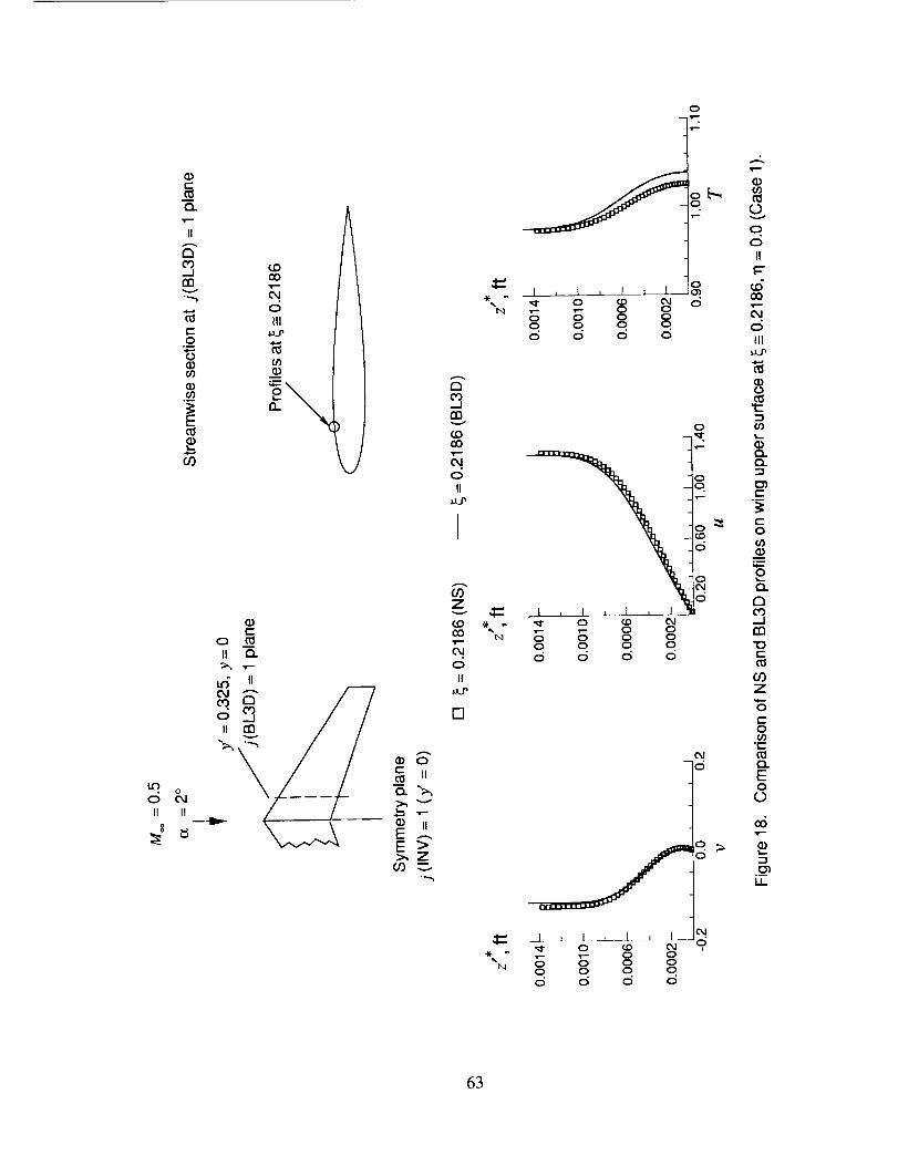
0
II
g
t-
Q.
II
D
n_v
-._,.
/-o
°_
E
II
00
o
a_
k;
II C_.
Lt_ tl0.1 "-"
d toII
F 7
/ ¢- 11
4--_ 'V"--
IIEE >>,7
-._
D
COv
¢.0cO
0
11
¢J)Z
¢£)co
C_l
0
II
[]
t_
N
c:)
I _ l i _ | I J_
o _ eJ do o o
o. o o o.o d o o
o
d[ I 1 I [ I I
0 0 O 0d d d o
._ • ..1--_ _1_ ___1__0 tad i'M
d d d d
o
d
04
o,
0
C_
0
_0
0
o
e--
e--0ffl
_.1en
f-
z,.e..-
0i--0
.i
e_E00
LI_
63
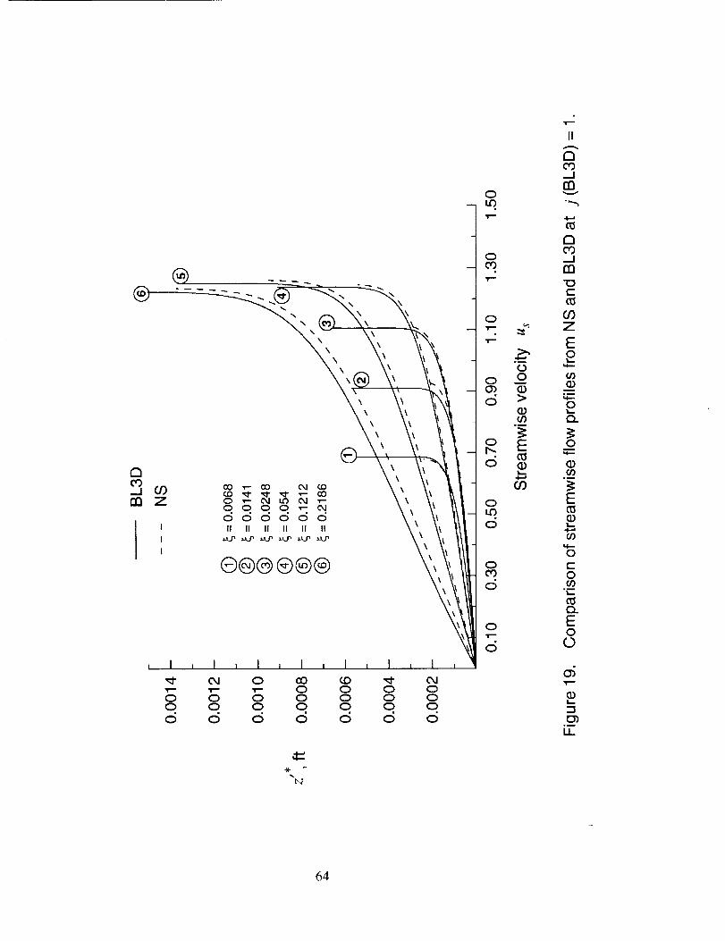
®
tncO_j tY)rn Z 0 T- Cxl _ _ T-
O 0 0 0 _-- 04
odoodII II II II II II
®@®®@®
I I
00
0
I l I l
0J 0 cO_ 0
0 0 00 0 0d d o
c.o0000
OOOd
o_1OOoO
OLO
O
O
O
d
od
o
O
OcOd
o
d
.m
oo
E
cO
II
r_COmlrnv
r_CO.._1m"Oc-
_0Z
EO
m.i
Oin
Q.
Oi
E
O0
Oc-O
.w
EOO
c_
LL
64

a03-Jrn
o
00d
CO _- CO O,I qD
qqoq_._ °0 0 0 0 0 0
II II II II II II
®@@®@®
cO0000
\
I , I , I ,
0 0 00 0 00 0 0
0 0 0
od
d
ooo
0
0
Od
!
O
o,
o
II
1210")_1rnv
121o')__1m
t--
r.OZ
E0
M,--
ffl
0
0
0
oI,I.,-
0c-0
E0
0
d
I.L
65

[]
n
[]
[] []
[]
[]
[][]
[][]
[]
[]0
[]
[]
D
0
n
0 0
LO-- Od
0
o
c_
oo
o_0
00
O0
I1
CO._1tY1v
IZItO.-Irn"13t-tO
COZ
Eo
(P
E
t-
U)"100c-
CIZ
0
0
0
0
t-O
a.
E00
0,1
q)Iw.
O_I.L
66
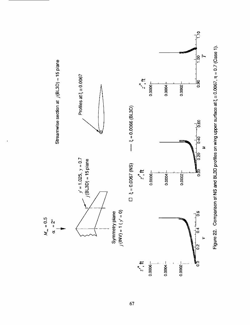
c-
Q.
H
D
m
c-O
¢D
E
o
0 ¢'xI
U II
8
o
J¢D
_ 0 0 0t'q 0 (_ 0
d d d
6'7

t-
O.
II
C_
nnv
E0
II II
8
E
o
t_
II
o o o I_
/I d d d III
°d _
_ -- - 0 .
_ o
0 E
N " oo g mo o
o
g
_1_ .l _ L_J_ I , _o._ " o o o
"t,_ 0 0 00 0 0cS cS d
6_
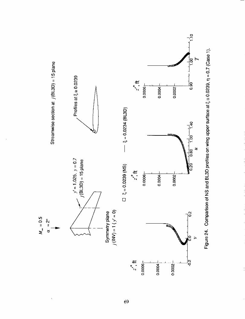
0
1.0
COII
0
o A_ Ill
v
._oo
(11.__
E
CO
o
0 _II II
121
env
0")
0
0II
o
o
c_II
- oo o° o_o o d
d d III
_ 0
* _ o o o"t_ o o o
o o od d d
69

II
r_
v
e-0.w
o
E
f#')
u_o
II II
8
o--T,-
oJ
_ _ ,_'" g o o
N O. o oo 6 d
70
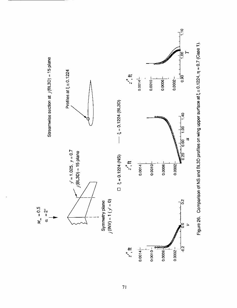
0
c
L_
II
O
v
c-O
o
L_o
II II
8
E
O0
D
v
c_II
II _ O0
J' _ •
. II
[]
g-,_E .-.E >:_Z
._1 ; I i I , 1 _
b-I 0 0 0 0
o o od o o o
'oo.i--
I , ] , I , Z0 _ C,,,I
','- 0 00 0 00 0 0 0d d d d
0
oo.
d
od
c_
!__±=_ 1 __:_ [
•== 0 00 0 00 0 0
d d
0
II
(M
o
o
e_
e--°--
e"om
o
e-I
121t_.._1en
Z
oe--o
._-t_
Eo
0
_d
.__u_
71
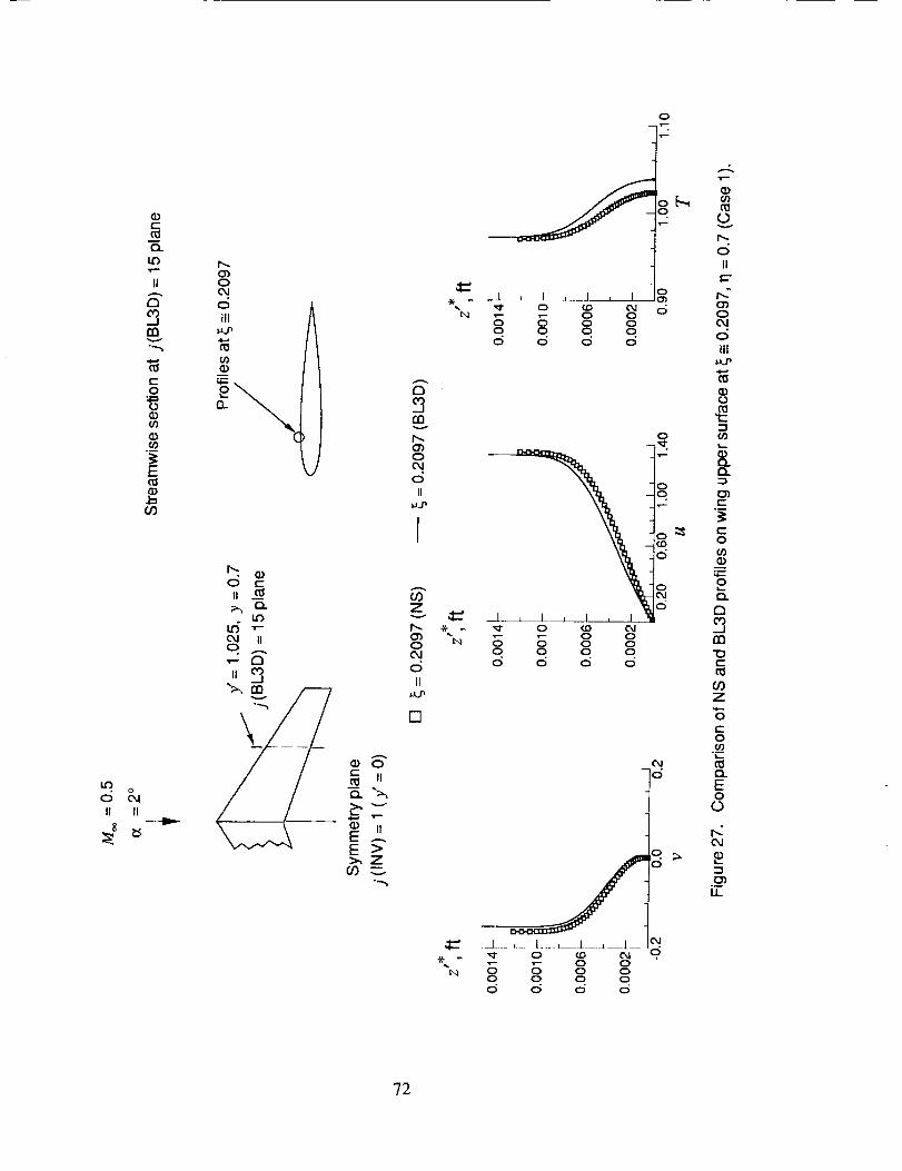
t-C_
Q.
Lt_
II
tn
en
0
Q
E
o00
kO
csII II
O_0OJ
0
t_
13-
c5 _It
o4 II0 ,._,,•,- D
If __.1
";_,m
\_ 0e-
llEE .-.E >
•...._
ood
o
I , _ I , I I°•,-- 0 00 0 00 0 0d o o
c',
rmv
o'_004
0
li
coZ
r-. _-O_o N
0
II
[]
o
_" 0 f_D•- 0 00 0 0 00 0 0 0o d d d
oo
c5
oc5
o
,.. _ _ 0 0L',-.1 0 0 0 0
0 0 0 0d d d
0v
II
0
o
Ill
o
Q.
c-O
U)
r_CO
m
_3c-
O_
Z
0
t-o00t-
Q.
E0
C)
r_c_
U_
72
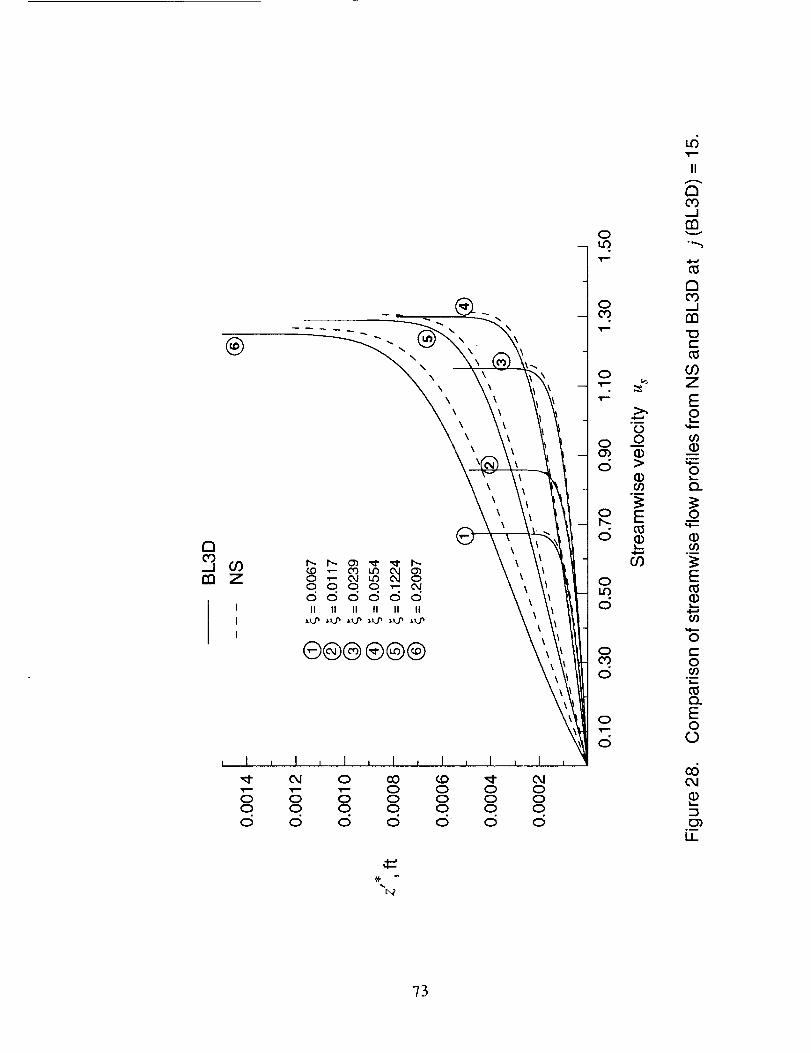
aCO_Jr_
®
®@@®@®
C_I O OO _ _" C_Iv- v-- v- O O O OO O O O O O OO O O O O O Od o d d d d d
_4
Ou3
Oco
O
O
d
od
o
O
O03d
o
d
.l-.a.m
oo
E
or)
Ld
II
CO
mv
C_CO_..I[]
"1:3c-
Z
EO
O
(3.
O
E
09
Oc-OO0.i
(3.EOO
0d
t33
II
73
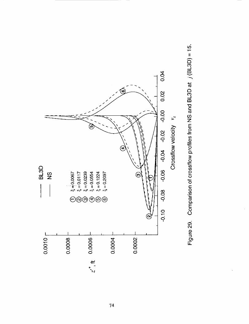
I i I0 cO_- 00 00 0d o
0 ",- 0_1 0o q o o,-.- _oodddo11 11 I1 11 II II
®@@®@®
\
d
Od
Ood
!
8
' OI-
Ot.oOd
!
coo
o
O
o,
II
Jrnv
n
Jm
"ot-
Z
EO
00u.m
Ot_
Om
Oo
Ot-O
.mib-
Q_EO
O
c_O4
II
74

atO
m Z
[]
[ !
0
[]
n
O'
O0
c_
[]
D
[]
[]
[]
[]
[]
[][]
[][]
rl[]
0[]
0
0
[]
[][]
[]
0 O O_0 ml" OJ
0
0
00
O0
L6
II
tO._Jrnv
nO0_Jrn
t-C_
cOZ
E,o
J_
E
C
"I0
0r-
rr
0
0
0
0
t-O00
O.
E00
d
IJ-
"75

CO
C_j
oO
O
O
O
O
c_'tz
O_Q.
(I)
o
"O
c_
(/3cD
u.I
¢.-
In
c_i
!
c_"0c--
o
0
-I0c0
c_
c_
L_
LL
76
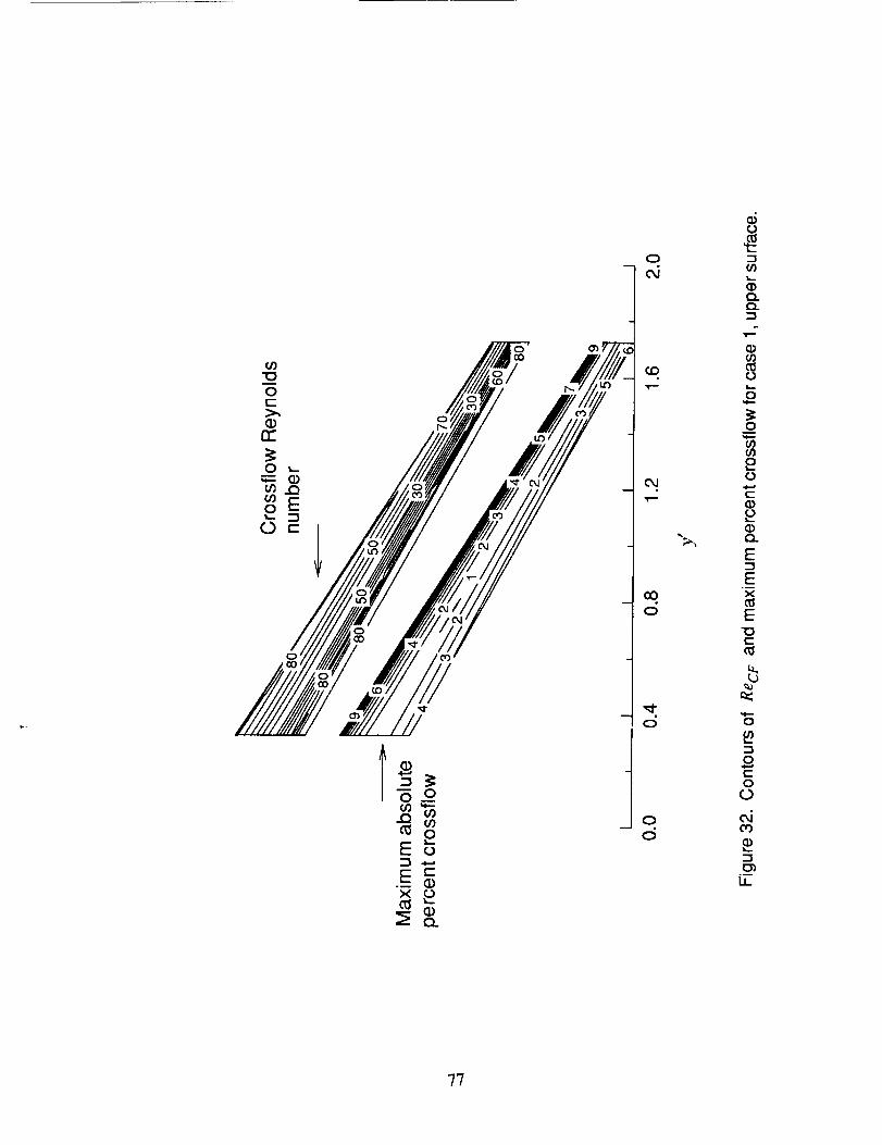
Q_
Q..
C_
O
Om
o
Q.
E
Exc_E
"Occ_
O
0
O
c_c_
c_
LL
77

q)
Q.
'T""
II
co
t--o
u)
q)
0 o4
II II
E
o__.T--
0
c_II
C_o
o
III
Eo
Iz}
_Jm
E
cOz
O
co
"E
e_EO
O
?8

I [] III
I !
OO
I
O
/I
IIII(
/
D
D
[]
D
o[]
\I c
// o
/ []/ n
/ o/ []
//
/
0 0
0C_l0
0
0
00
O0
0
(./)
1.0
II
aco_.1rn
Dco_Jrn
"0c-
O0Z
Eo
E
cz0')"ooc->,
n-
o
u_u_o
0
oc-O09
c_O.EOO
0--
79
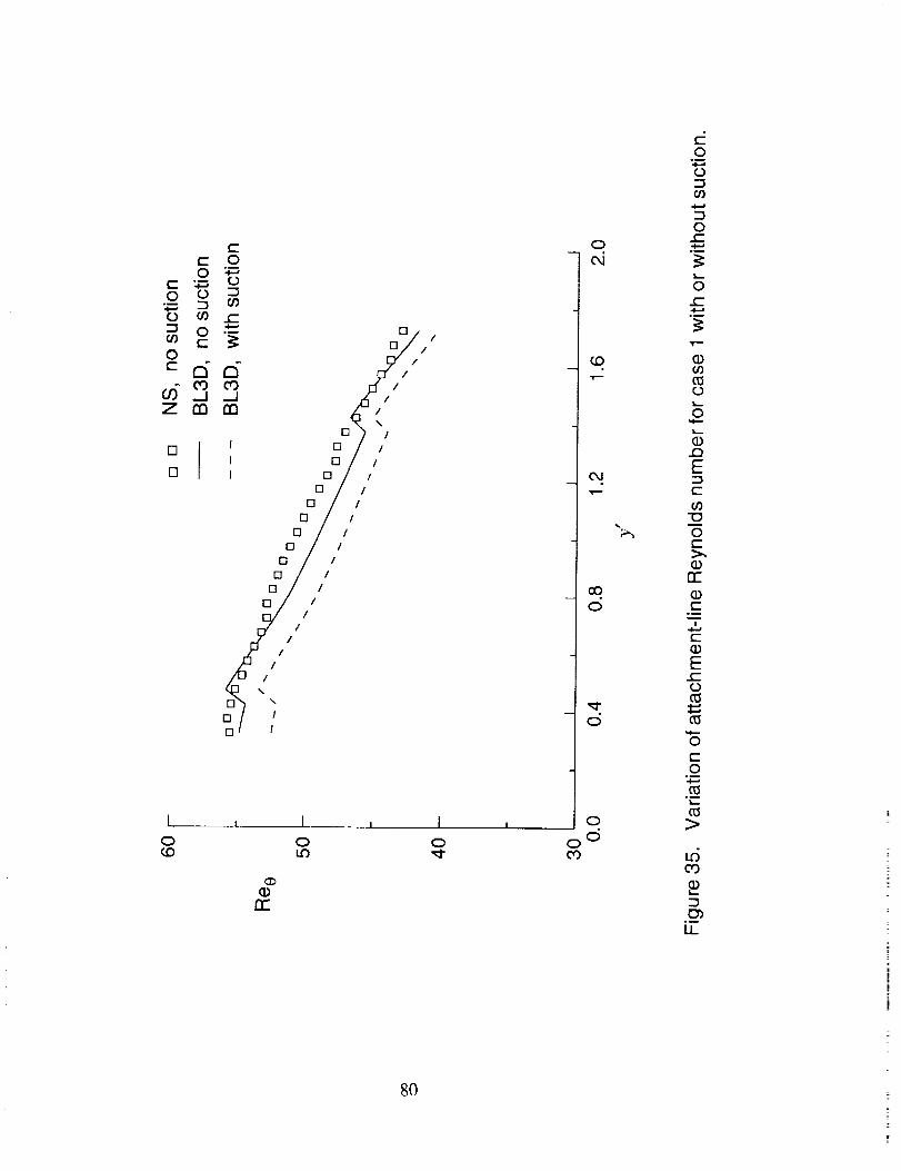
Cc 00
0
=Sd--1 J
Z rn rn
[] II
[] I
[][3[]
[][]
[] /13 /
[] /o /
D /[] /
[] !O /
!/
//
/%
[] \II
[][]
//
//\
I/
/I
I
I
I
I
I0_D
rr"
I
0LO
I0 0
03
80
0
O4
_O
Od
00
0
0
00
d0
O
O
O
O
O
(D.O
E(-
00"O
O(.-
rr-
C
C
Ec-O
O¢..O
u5CO
LL

L._
ii
>Z
c-O
0i
ioo
, i ,oo
,i
"_ "_ I"--
II II I1
> > >Z Z Z
I i J I
o (Do 0
G)0Lo
oo
o°
ooc_
o-- 0
w--
e_
0")
0
E0(1)C_(D
oi
c-OtO
(DC_
cO
0'4--
"0.i
C_
(Di
-sU2
CO
(D
C_°_
LL
81
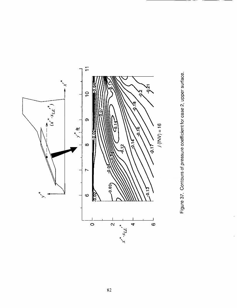
T B
I J I i
*
_OT m
II
Zmv
vC
T,B
Q.Q.
c_
0
C
0
--I
OL
0
_D
0
C
0c_
r<cO
0
Z_
LL
82

LOII
aO3_.1
c-O
C
0..00
].j 'e6pe 6u!peel leOOl o_,eA!].eleJ ,,:_
_ _ _ 0o o d o o
I I I ' tl ' I I I
\I
_ _ _
Illltl d0 0 0 0 00 0 0 0 0
_ 0 _
o _ o d o,
0
o.
o
0
E£
oi--
!
ai
o
._-
13O3Jrn0
13
0I3.
e-
roZl=
00
13_"
o5O3
Cr_LL
$3

c-O
.m
0
C
(D
LI.I
(.-0
.m
00')
ILl
r'lU..I
I-.Irn
0
II
>Z
00
01.0'm"
00
.)(-
0
G_
00
O
c-O
.m
0
U.I
121Iii
I-.Irn"0r-
ILl
E0
0
if)
0
c-O0
0
t-O
E00
LI_
84
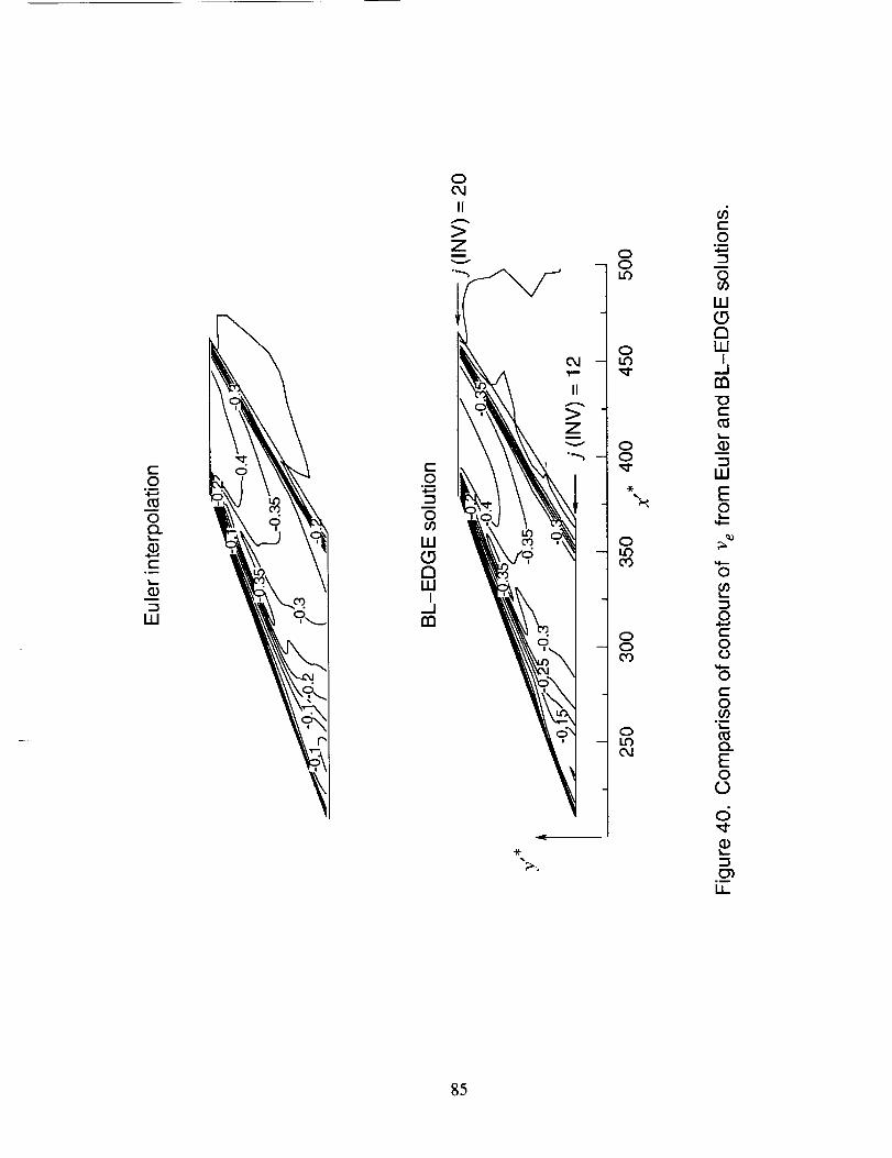
t-O
°u
0tn
ot-
LLI
t-O
0
LO0DLLi
I_ln_
0
II
Z
-K-
II
Z
0- 0
L_
0
00
0
CO
00CO
0I._
C0
i--
0_0
W0rnU.l
I_lr_
t-
O
W
EO
M',,,,-
O
O
CO
Ot-O
.r--
Q.
EO
o
d
1.1_
85
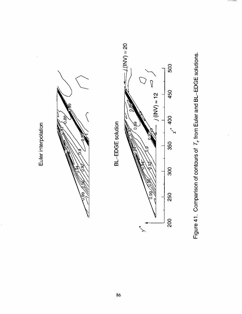
t-O
°m
OQ_
t-
L.
t-O.i
O
W(DnIllI
..Jrn
O-- O
u9
O
OO_-
OLOCO
OOO3
OLO
OOOJ
_6t-O
.i
OO9
LU(DtnIllI
..J
nn"Ot-
CD
Ill
EO
O
_0
O
t-O
O
t-O
tn
EO
CD
(D
II
86

0o
o
c_
o0")o
0o
I
oo
O
I=
(/)
Q.a.
oor)
o
o°_
O
W
O.m
O
W
rnW
I
nn
O
O
.m
Q.EOO
.o
U_
87

1,1,1,1,. O _ O
o o o od d d d
o
O
-o
, o u'_ o un doJ _ _ o"1_ o o o o
o o o _z)c5 c_ d d
OJ _ O
"_ o o _ oO O O
d d d d
CO--O
d
d
d
d
d
o
co
Eo
o
u0co
oII
CO O.J OJ ','- O__O "'lx_ O O O O _ O
O. O. O O O Oe9 o o o o d oQ.o
i.o
oo
II
o"ooo
aco_Jn_
o
c_
CO 04 O,I ",-- O'_ O O O O O O
O O O O O O
d d d d d d
,DO
oq'ID
o !o
oO
o
:30_
[] , O _ O _ O _ d_ O_I _ 0
[] "_ o o o o _ oO O O O O
d d d d d d
O_
OJ
O
II
t-
COO
O
II
O
O
O
0O
.m
O
tn
t-O
.i
O00
Ot-O0O
.i
EO
O
o5
I..L
88
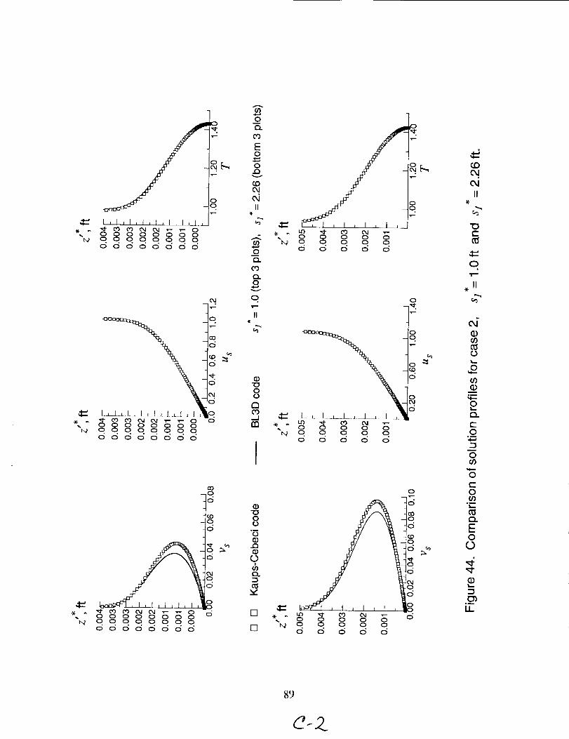
I , I , I , I , I , I L I , I_._J
0 0 0 0 0 0 0 0"_b2 0 0 0 0 0 0 0 0
dddodddd
___000000000
_00000000
dddddddd
0
OEI
d
c5
dO4
d
R0
.)(. . _I" _ _ C_i L_J _ _-- 0• _ 0 0 0 0 0 0 0 0
ix? 0 0 0 0 0 0 0 0
dddddddd
CO{:3
d
d
d
0
(/)oEl.
Eo
o..ov
t,OO,IOaII
tag0O.
tOt'_0
0
II
o
oo
¢0_Jn7
0
oo
oo
o0
[]
[]
0 0 0_1"_ 0 0 0 0 0
d o o d d
oF.,
o
0
"lx_ 00
Lr) _1" e') 0,10 0 0 0 0
o o o o.0 0 0 0
LF) _ O') 0,10 0 0 0
'_1'-4 0 0 0 0 0d d d d d
O
o
c_
od
od
, gd
r4_
OJII
E
O
11
O00
O
o00O
,m
O
EO
.n
O
O
O
Eoo
o
o_
LL
89

0
[] / "g 7_
[] _ .,= 4
--- ° v m
Oo\
I t I , I ,0 0 0 0 0 0 0 0 0 0 0 0 00 0 0 0 0 0 0 0 0 0 0 00,.I _ 0 O_ CO I_ _D _ _ CO 0.1 ',--
oJ(D0_
o
0
II
c)cO.Jrnv
00
CD
E
e-0_"00e-
rr
ou
¢J0¢,00o
0c-O
._-
O.E00
U_
9O

Appendix A
Coefficients of the Linearized System of Compressible Three-Dimensional
Boundary-Layer Equations Discretized With a Fourth-Order Pade Formula
(1) Coefficients of Continuity Equation:
alkl = --I
akl2 = --Clk(Cll)k_ 1
akl3 = --Clk@12 )k_ 1
akl4 = 0
akl5 = --C2k(ell)k_l
a_ = --_k(_l_)k-1a_7 = 0
b_l = 1
b_2 = --Clk@ll) k
b_3= -_1k(_12)kb_4 = 0
b_6 = C2k(el2)k
b_7 = 0
r_ =--(qll)k+(qll)k_l A-Clk(ql2)k+elk(ql2)k_l -- e2k(q13)k-t-C2k(q13)k_l
qll = W
ql_ = A1F_ + A2F + A3G, 1 + A4G
q13 = A1L( + A2L + A3M, 1 + A4M
Cll = alA] + A2
e12 = blA3 + A4
1A_clk = _- _,_
A-1

(2) Coefficients of _ Momentum Equation:
a2kl = Fk-1
a2k2 = Wk-1 -- Clk(e21)k-1 -- C2k(e22)k-1
ak3 = --Clk(623)k_ 1 -- C2k(e24)k_ 1
ak4 = --¢lkB6
ak 5 -- --lk_l -- C2k(e21)k_l
bk22 = --Wk -- Clk(e21)k -4- C2k(e22)k
bk23 = --¢lk(e23)k 3L C2k(e24)k
bk4 = -c]k B6
b2k5= tk + c2k(e21)kb2k6= c2k(*23)kb2k7= c2k_6
r2k = --(q21)k -I- (q21)k-i -1- Clk(q22)k -F Clk(q22)k_l --C2k(q23)k -1- C2k(q23)k_l
q21 = (1L - wF)
q22 = B1 (F2)_ + B2(FG)u +/_3F 2 + [34FG +/35G 2 +/_6H
q23 = 2BI(FL)_ + B2(FM + GL),_ + 2[_3FL + B4(FM + GL) + 2115GM + [3_I
e23: (blB2-t-B4)F+2[_sG
A-2
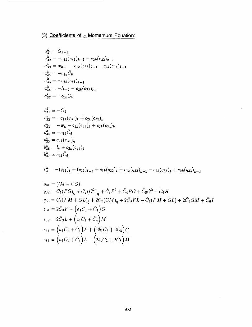
(3) Coefficients of _ Momentum Equation:
ak31 = Gk_ 1
ak32 = --Clk(e31)k_ 1 -- c2k(e32)k_ 1
ak33 = wk_ 1 -- Clk(eZZ)k_ 1 -- C2k(eZ4)k_ 1
ak34 = --clkC 6
ak35 = --c2k(e31)k_ 1
a_ = -c2kdo
b3kl =-Gk
b3k3= -wk - _lk(_33)k+ _2k(_34)_b3k4= -_1_d6b3_5= ¢2_(_31)kbk36 = lk "4- C2k(e33)k
bk37= _2kd6
r_ = --(q31)k+(q31)k_l-t-Clk(q32)k+Clk(q32)k_l --C2k(q33)k-t-C2k(q33)k_l
q31 = (IM - wG)
q32= C,(FC)_+ C2(C2),q33 =
e31 --
e32 =
633 =
¢34 =--
+ C3F 2 + C4FG + C'sG 2 + C'6H
CI(FM + GL)_ + 2C2(GM), 1 + 2CaFL + C4(FM + GL) + 2CsGM + C6I
(o, 12C3L -4- (alCl-t-C4)M
(alC1-4-C4) FnL (2blC2-Jc2C5)_
(alCI-FC4)L+ (261C2-1-2C5)"
A-3
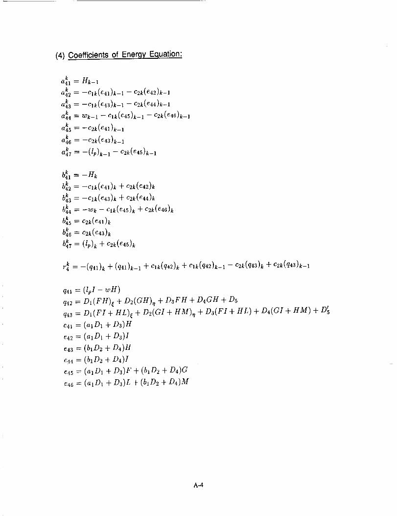
(4) Coefficients of Energy Equation:
a_l = Hk-1
a_2 = --Clk(e41)k_ 1 --C2k(e42)k-1
a_3 = --Clk(e43)k_l --C2k(e44)k-1
a_4 = Wk_l--Clk(e45)k_ 1 --c2k(e46)k-1
a_5 =--C2k(e41)k_l
a_6 = --C2k(e43)k_ 1
bkl = -Hk
b4k2= -_k(.41)_ + c2k(.42)_
bk43 = --Clk(e43)k + C2k(e44)k
b_ = -_k - _k(_4_)k+ _2k(_46)k
b_7= (lp)k+ _2k(_45)k
r_ -- --(q41)k+(q41)k_l-l-Clk(q42)k+Clk(q42)k-l--C2k(q43)k -t-c2k(q43)k-1
q41 = (lfl - wH)
q42 = DI(FH)_ + D2(GH), I
q43 =
e41 _---
e42 --'--
e43 =
C44 =
C45 _---
e46 =
+ D3FH + D4GH + D5
DI(FI + HL)_ + D2(GI + HM)_ + D3(FI + HL) + D4(GI + HM) + 015
(aiD1 + D3)H
(aiD1 + D3)I
(biD2 + D4)H
(biD2 + D4)I
(aiD1 + D3)F + (biD2 + D4)G
(aiD1 + D3)L + (biD2 + D4)M
A-4
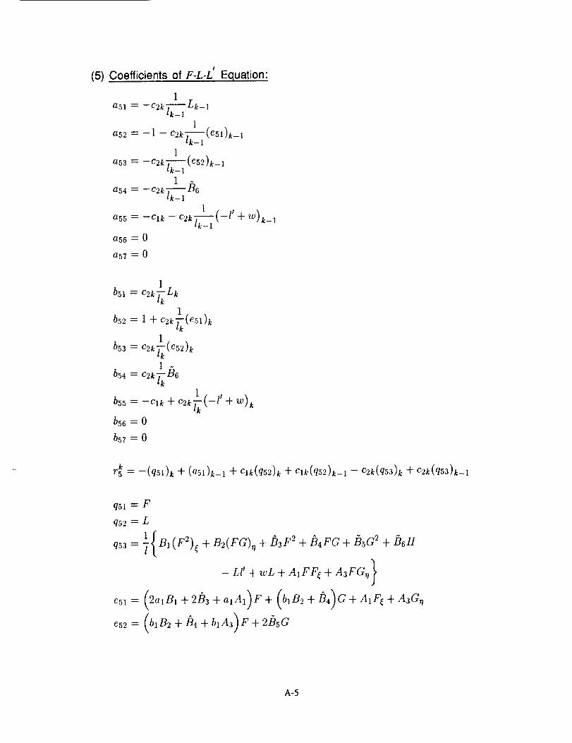
I
(5) Coefficients of F-L-L Equation:
a51 =
a52 =
a53 =
a54 =
a55 =
a56 =
a57 =
--C2k l-__l Lk-1
1
-1 - c2k1--__l(_sl)__11
--C2kl__l(e52)k-1
1 (--l'+wlk_l--Clk -- C2k __lk--_
0
b51 = C2k_kLk
1
bs_= 1+ c2k_(e51)k
b53 = C2k_-_(e52)k
b54 = C2k B6
b55 = --elk -_- C2k _--_(--l' A- W)k
b56 = 0
b57 = 0
r_ = --(qS1)k+(OS1)k_l +Clk(q52)k+Clk(q52)k_l--C2k(q53)k+C2k(q53)k-1
q51 = F
q52 = L
1{q53 = _ BI(F2)_ + B2(FG)_ +/?3F 2 + B4FG +/_sG 2 +/)6H
- Ll' + wL + A1FF_ + A3FG,}
651 --_ (2al"l 7L2[_3-_-alA1)F-_ (blB2-_-[_4)G-_-A1F,_-A3 G71
652 : (biB2-_- [_4 -4- blA3)F -_- 2B5G
A-5

I
(6) Coefficients of G-M-M Equation"
a61 = --C2k-].Z_1k-1lk-1
a62 = --C2k _ l--'_-(e61)k_l%-1
1
a65 = 0
1 i_ = -c,_ - c_l-__(-l +_)_-1a67 = 0
b_l = c2k_Alk
b62= c2k¼(_6a)k1
b63 = 1 + c2k_(e62)k
b_4 = c2kld6tk
b65 = 0
b66 = --Clk -t- C2k _-_(--l' "4- W)k
b67 = 0
rk = --(q61)k q- (q61)k-1 q- Clk(q62)k + Clk(q62)k-1 -- C2k(q63)k+C2k(q63)k-1
q61 : G
q62 = ._I
1{q63 = 7 CI(FG)_ + c_(c_). + d_r 2+ d_Fc + d_c 2+ d_H
- Ml' + wM + A1GF_ + AaGGu_)
¢61 = 2(_3F + (a,C, + C4 q-alA1)G
e62= (alCI+C4)F+(2blC2+2Cs+blA3)G+AIF,+A3Grl
A-6

!
(7) Coefficients of H-I-! Equation:
a71 = --c2k (lp)k_ 1--Wk_ 1
1
a72 = -_2k (lp)__1(_71)k-11
1= -1 - c2k_(_73)k_la74
t I I
_'P]k-1
a75 =0
a76 ---- 0
1.77 = -_1_ - _2k,I _ (-l_ + w)_-x
k'P]k-I
1
571 ---- C2k(_v)tWkP)k
1
b72 =-- C2k (_._L(e71)k
1b73 = C2k--(e72)k
(lp)k1
b74 = 1 q- C2k._-'_-_---.(673) k(lp)k
b75 = 0
b76 = 0
1b77 = -clk + c2k--(-lp + w)k
(Ip)k
rk = --(q71)k + (q71)k-1 + Clk(q72)k + Clk(q72)k-1 -- C2k(q73)k + c2k(q73)k-1
q71 = H
q72 = I
q73 = _-_{DI(FH),+ D2(GH). + D3FH + D4GH + D5
- II'p + wI + A1HF_ + A3HG,_}
e71= (a,D, + [93 + a]A1)H
e72 = (blD2 -4- [_4 + blA3)H
e73= (alDI+D3)F+ (blD2+£)4)G+A1F_+A3Go
A-7


Appendix B
User's Manual for the BL3D Program
The BL3D program package consists of a collection of program files, input files, and
output files that relate to the solution of three-dimensional boundary-layer flow on a swept
wing. In addition to the BL3D program files, the program package includes files related
to the Euler and Navier-Stokes calculations for the two example cases and the interface
programs. Some of these files are not directly related to the core program BL3D, but
were developed for the validation of the code. These include Euler and Navier-Stokes
grid and solution files as well as programs used in processing the Navier-Stokes results
for comparison with the BL3D results. All the files have been archived on the NASA
Langley Masstor system and can be made available per individual request.
Table 1 at the end of this section gives a list of important computer variable names
used in the programs and the corresponding translation to the variables used in the
formulation as listed in "Nomenclature". This list may be useful for customizing the
program for a particular application.
Program Structure
The files are divided into subdirectories as follows. Each subdirectory contains a
README file with a short description of the contents of the subdirectory and instructions
for running the programs.
bl3d/euler/casel. Contains files that correspond to generation of the Euler
solution for case 1 (subsonic swept wing) with the code CFL3D. The program CFL3D
is not included.
bl3d/interface/casel. Contains interface programs and input files used in
processing the Euler solution for case 1 and generation of the data file required in the
BL3D run.
B-I,
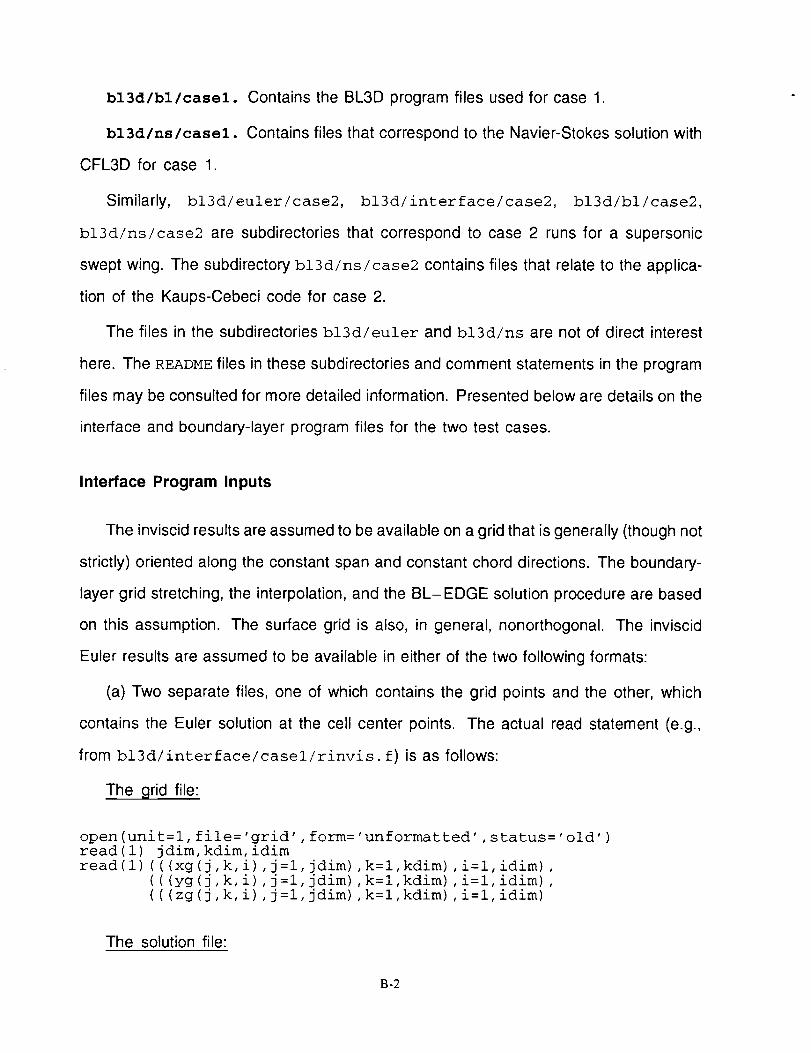
bl3d/bl/casel.
bl3d/ns/casel.
CFL3D for case 1.
Contains the BL3D program files used for case 1.
Contains files that correspond to the Navier-Stokes solution with
Similarly, bl3d/euler/case2, bl3d/interface/case2, bl3d/bl/case2,
bl3d/ns/case2 are subdirectoriesthatcorrespond to case 2 runs for a supersonic
swept wing. The subdirectory bl3d/ns/case2 contains files that relate to the applica-
tion of the Kaups-Cebeci code for case 2.
The files in the subdirectories bl3d/euler and bl3d/ns are not of direct interest
here. The README files in these subdirectories and comment statements in the program
files may be consulted for more detailed information. Presented below are details on the
interface and boundary-layer program files for the two test cases.
Interface Program Inputs
The inviscid results are assumed to be available on a grid that is generally (though not
strictly) oriented along the constant span and constant chord directions. The boundary-
layer grid stretching, the interpolation, and the BL-EDGE solution procedure are based
on this assumption. The surface grid is also, in general, nonorthogonal. The inviscid
Euler results are assumed to be available in either of the two following formats:
(a) Two separate files, one of which contains the grid points and the other, which
contains the Euler solution at the cell center points. The actual read statement (e.g.,
from bl3d/interface/casel/rinvis, f) is as follows:
The grid file:
open(unit=l,file='grid',form='unformatted',status='old')read(l) jdim, kdim, idim
read(1) (((xg(j,k,i),j=l,jdim),k=l,kdim),i:l,idim),
(((yg(j,k,i),j=l,jdim),k=l,kdim),i:l,idim),
(((zg(j,k,i),j=l,jdim),k=l,kdim),i=l,idim)
The solution file:
B-2
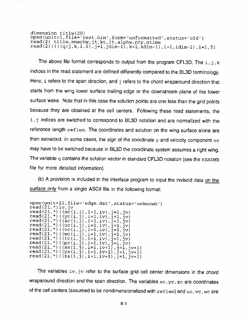
dimension titlw(20)
open(unit=l,file='rest.bin',form='unformatted',status='old,)
read(2) titlw, xmachw, jt,kt, it,alphw, ntr,ntime
read(2) ((((q(j,k,i,l),j=l,jdim-l),k=l,kdim-l),i=l,idim-l),l=l,5)
The above file format corresponds to output from the program CFL3D. The i, j, k
indices in the read statement are defined differently compared to the BL3D terminology.
Here, i refers to the span direction, and j refers to the chord wraparound direction that
starts from the wing lower surface trailing edge or the downstream plane of the lower
surface wake. Note that in this case the solution points are one less than the grid points
because they are obtained at the cell centers. Following these read statements, the
i, j indices are switched to correspond to BL3D notation and are normalized with the
reference length reflen. The coordinates and solution on the wing surface alone are
then extracted. In some cases, the sign of the coordinate y and velocity component vc
may have to be switched because in BL3D the coordinate system assumes a right wing.
The variable q contains the solution vector in standard CFL3D notation (see the README
file for more detailed information).
(b) A provision is included in the interface program to input the inviscid data on the
surface only from a single ASCII file in the following format:
open (uniread (2 I,
read (2 i,
read(21,*) (
read(21,*) (
read(21,*) (
read(21,*) (
read(21,*) (
read(21,*) (
read(21,*) (
read(21,*) (
read(21,*) (
read(21,*) (
t=21, file='edge.*)iv, jv
*) ((xc(i,j) ,i=l,
(yc(i j) ,i=l,
(zc(i j) ,i=l,
(uc(i j) i=l
(vc(i j) i=l
(wc(i j) i=l
(tc(i j) i=l
(pc(i j) i=l
(xs(i j) i=l(ys(i j) i=l
(zs(i j) ,i=l
dat',status='unknown')
iv)
iv)
iv)
iv)iv)
iv)
iv)
iv)
j=1 iv)j=1 iv)j=1 jr)j=1 iv)j=1 iv)j=1 iv)j=1 iv)j=1 iv)
iv+l) ,j=l, jv+l)iv+l) ,j=l, jv+l)
iv+l) ,j:l, iv+l)
The variables iv, jv refer to the surface grid cell center dimensions in the chord
wraparound direction and the span direction. The variables xc, yc, zc are coordinates
of the cell centers (assumed to be nondimensionalized with reflen) and uc, vc, wc are
B-3
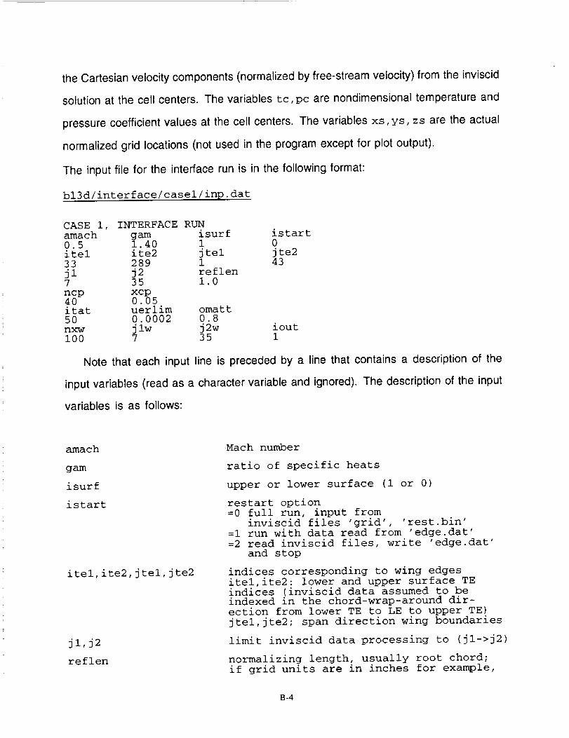
the Cartesian velocity components (normalized by free-stream velocity) from the inviscid
solution at the cell centers. The variables tc,pc are nondimensional temperature and
pressure coefficient values at the cell centers. The variables xs, ys, zs are the actual
normalized grid locations (not used in the program except for plot output).
The input file for the interface run is in the following format:
bl3d/interface/casel / inp. dat
CASE i, INTERFACE RUNamach gam isur f is tar t0.5 1.40 1 0itel ite2 jtel jte233 289 1 43
jl j2 reflen7 35 1.0
ncp xcp40 0.05itat uerlim omatt50 0. 0002 0.8
nxw j lw j 2w iouti00 7 35 1
Note that each input line is preceded by a line that contains a description of the
input variables (read as a character variable and ignored). The description of the input
variables is as follows:
amach
gam
isurf
istart
itel,ite2,jtel,jte2
jl,j2
reflen
Mach number
ratio of specific heats
upper or lower surface (i or 0)
restart option=0 full run, input from
inviscid files 'grid', 'rest.bin'
=i run with data read from 'edge.dat'
=2 read inviscid files, write 'edge.dat'
and stop
indices corresponding to wing edges
itel,ite2: lower and upper surface TEindices (inviscid data assumed to beindexed in the chord-wrap-around dir-
ection from lower TE to LE to upper TE)
jtel,jte2; span direction wing boundaries
limit inviscid data processing to (jl->j2)
normalizing length, usually root chord;
if grid units are in inches for example,
B_
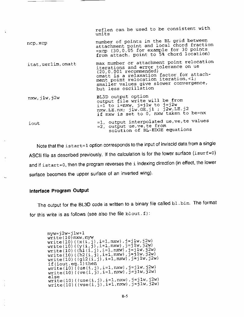
ncp,xcp
itat,uerlim, omatt
nxw, jlw, j2w
iout
reflen can be used to be consistent withunits
number of points in the BL grid betweenattachment point and local chord fraction=xcp (30,0.05 for example for 30 pointsfrom attach, point to 5% chord location)
max number or attachment point relocation
iterations and error tolerance on ue
(20,0.001 recommended)omatt is a relaxation factor for attach-
ment point relocation iteration,<l;smaller values give slower convergence,
but less oscillation
BL3D output option
output file write will be fromi=l to i=nxw, j=jlw to j=j2w
nxw. LE.nx; jlw. GE.jl ; j2w. LE.j2if nxw is set to 0, nxw taken to be=nx
=i, output interpolated ue,ve,te values
=2, output ue,ve,te fromsolution of BL-EDGE equations
Note that the istart=l option corresponds to the input of inviscid data from a single
ASCII file as described previously. If the calculation is for the lower surface (isurf=0)
and if istart=0, then the program reverses the i indexing direction (in effect, the lower
surface becomes the upper surface of an inverted wing).
Interface Program Output
The output for the BL3D code is written to a binary file called bl.bin. The format
for this write is as follows (see also the file blout, f):
nyw=j 2w- j lw+lwrite (i0 )nxw, nywwrite(10) ((x(i,j),i=l,nxw),j=jlw, j2w)
write(10) ((y(i,j),i=l,nxw) ,j=jlw, j2w)
write(10) ((hl(i,j),i=l,nxw),j=jlw, j2w)
write (I0) (write (i0) (
if (iout. eqwrite (i0) (
write (i0) (elsewrite (i0) (
write (I0) (
(h2 (i, j ) ,i=l, nxw) ,j=j lw, j2w)
(g12 (i, j) ,i=l,nxw) ,j=j lw, j2w)
.i) then(ue (i, j ) ,i=l, nxw) ,j=j lw, j2w)
(ve (i, j ) ,i=l, nxw) ,j=j lw, j2w)
(use (i, j) ,i=l, nxw) ,j =j lw, j2w)
(vse(i,j) ,i=l,nxw) ,j=jlw, j2w)
B-5
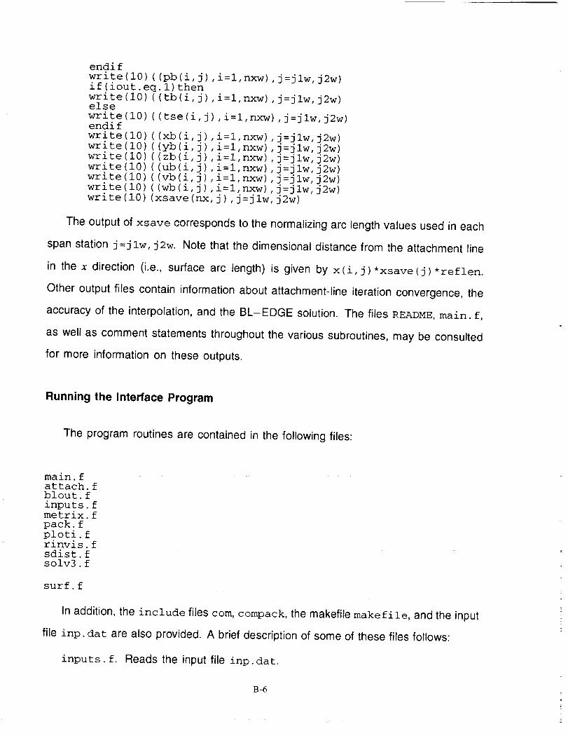
endi fwrite(lO) ((pb(i,j),i=l,nxw),j=jlw, j2w)if (iout. eq. i) thenwrite(lO) ((tb(i,j),i=l,nxw),j=jlw, j2w)elsewrite (i0)endi fwrite (I0 )write (i0 )write (i0)write (I0)write (i0)write (i0)write (i0)
((tse(i,j),i=l,nxw),j=jlw, j2w)
((xb(i,j),i=l,nxw),j=jlw, j2w)( (yb (i, j ) , i=l, nxw) , j:jlw, j2w)( (zb(i, j) , i=l, nxw) , j=jlw, j2w)( (ub(i, j) , i=l, nxw) ,j=j lw, j2w)( (vb(i, j) ,i=l, nxw) ,j=j lw, j2w)
((wb(i,j),i=l,nxw),j=jlw, j2w)
(xsave (nx, j ) ,j=jlw, j2w)
The output of xsave corresponds to the normalizing arc length values used in each
span station j=jlw, j2w. Note that the dimensional distance from the attachment line
in the x direction (i.e., surface arc length) is given by x (i, j ) *xsave (j) *reflen.
Other output files contain information about attachment-line iteration convergence, the
accuracy of the interpolation, and the BL-EDGE solution. The files README, main. f,
as well as comment statements throughout the various subroutines, may be consulted
for more information on these outputs.
Running the Interface Program
The program routines are contained in the following files:
main. fattach.fblout.f
inputs.fmetrix.f
pack. f
ploti.frinvis.fsdist.fsolv3.f
sur f. f
In addition, the include files corn, compack, the makefile makefile, and the input
file into. dat are also provided. A brief description of some of these files follows:
inputs.f. Reads the inputfile inp.dat.
B-6

rinvis, f. Reads the inviscid data; extracts required data needed for the upper or
lower surface; normalization of coordinates and flow quantities.
attach, f. Locates the initial attachment line (for first pass only); generates a
boundary-layer surface grid that originates from the currently defined attachment line;
calls sdist, f for a suitable grid stretching.
metrix, f. Calculates metric quantities hi, h2, g12 based on currently defined
boundary-layer grid.
surf. f. Solves the BL-EDGE equations if this input option is selected.
blout, f. Outputs the file bl.bin required for BL3D run.
pack. f. Library of cubic tension spline interpolation routines.
The include file corn has the following parameter statements (which correspond to
case 1 in this example):
parameter(jdim=321,kdim=49,idim=53)
parameter(ivm=257,jvm=43)
parameter(nxm=3OO,nym=jvm)
The dimensions depend on the inviscid grid size and the boundary-layer grid size;
see comment statements in the file corn for selection of these values.
The include file compack is used in conjunction with the spline routines in pack. f.
The program is run as follows: choose appropriate dimensions in the parameter
statements in the file corn; remove all. o files if corn is modified; then type make followed
by a. out to run the program. The output files fort. 3, fort. 20, fort. 30, fort. 31,
fort. 32, fort. 50, fort. 51, fort. 99 are useful for plotting or checking the results.
Please refer to the various subroutines for a description of these outputs.
An appropriate selection of input quantities and inviscid data of good resolution are
required for successful completion of the interface run. Run times on the Cray are only a
B-7
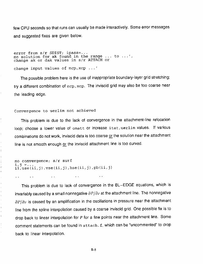
few CPU seconds so that runs can usually be made interactively. Some error messages
and suggested fixes are given below.
error from s/r SDIST; ipass=...
no solution for ak found in the range ...
change ak or dak values in s/r ATTACH or
to• • • ;
change input values of ncp,xcp ...'
The possible problem here is the use of inappropriate boundary-layer grid stretching;
try a different combination of ncp, xcp. The inviscid grid may also be too coarse near
the leading edge.
Convergence to uerlim not achieved
This problem is due to the lack of convergence in the attachment-line relocation
loop; choose a lower value of omatt or increase itat,uerlim values. If various
combinations do not work, inviscid data is too coarse 9_[the solution near the attachment
line is not smooth enough or the inviscid attachment line is too curved.
no convergence; s/r surf
i,j =...ii,use(ii,j) ,vse(ii,j) ,hse(ii,j) ,pb(ii,j)
• • • • • • • • • •
This problem is due to lack of convergence in the BL-EDGE equations, which is
invariably caused by a small nonnegative coP/oqx at the attachment line. The nonnegative
OP/Ox is caused by an amplification in the oscillations in pressure near the attachment
line from the spline interpolation caused by a coarse inviscid grid. One possible fix is to
drop back to linear interpolation for P for a few points near the attachment line. Some
comment statements can be found in attach, f, which can be "uncommented" to drop
back to linear interpolation.
B-8

Boundary-Layer Program Inputs
The inputs to the boundary-layer program are composed of two files:
(a) The boundary-layer edge data file bl. bin. This binary file is created by running
the interface program and is assumed to be available in the current directory (bl/casel,
for example). The format for this file has been described previously. This file is read
in the subroutine rinvis.
(b) The boundary-layer input options file inp. dat. This file is read in the subroutine
inputs and is assumed to be in the following format (note that each input line is
preceded by a line that contains a description of the input variables, which is read as
a character variable and ignored):
bl3d/bl/casel/inp.dat
CASE 1 : BL INPUTSAMACH PFS TFS PRL IWALL0.5 2000 520 0.72 0
ZMAX AK NXLIM NYLIM8.0 1.05 68 29ITMAX EPSF EPSG EPSH IORD
20 l.e-6 l.e-6 l.e-06 5
The description of the input variables is given below:
REFLEN I_IT1.0 0
amach
pfs
tfs
prl
iwall
reflen
free-stream Mach number
free-stream static pressure (lb/ft2)
free-stream static temperature (deg R)
laminar Prandtl number
wall boundary condition=0 adiabatic wall
=i wall temperature, deg R specified(read in 'main. f')
=2 wall heat flux specified ,ib/(ft.sec)
(read in main.f)
note: suction rates are also specified in
reference length in ft.(similar to input in interface program, but
'main.f'
in ft.)
B-9

iunit
zmax
ak
nxlim
nylim
itmax
epsf
epsh
iord
US or SI units, =0 for US units
SI units not currently implemented
maximum value of transformed variable
corresponding to boundary-layer edge
stretching coefficient by which points are
distributed away from the wall
number of stations to march in x direction
number of span-wise stations in y direction
maximum number of iterations at each (i,j)
convergence criterion for f-prime at wall
convergence criterion for h-prime at wall
value of i for which scheme becomes fully
order in the stream-wise direction
'zeta'
point
second-
Boundary-Layer Program Outputs
The output from the boundary-layer program is output to several fort. files. The
convergence information can be found in fort. 2. Most of the results are output from
subroutine phys and can be modified as required. The output quantities include
z*, u, v, 7" profiles; boundary-layer thickness, displacement thickness, and skin-friction
coefficient; streamwise and crossflow profiles; and crossflow Reynolds number. Please
refer to subroutine phys for more details. Note that these "writes" are for each (i,
j) location (with j as the inner loop).
Output Format for Stability Analysis
The output of profiles and their derivatives to first and second order, as well as
edge-normalizing quantities, are made in the format described below.
open(unit=7,file='fort.7'
write(7)title
Title in character*80.
,form='unformatted',status='unknown')
B-IO

write(7)nxlim, nylim, reflen
nxlim is number of chordwise stations.
nylim is number of spanwise stations.
reflen is reference length, dimensional.
write (7) pfs, tfs, ufs, amach, rofs
Quantities P_o, T_o, U_o, Moo, p*.
For each profilei=l,nxlim; _=l:nylim:
write (7)i,j,nz,x(i,j),y(i,j) ,xbs,ybs,zbswrite (7)hl(i,j),h2(i,j),gl2(i,j) ,sls
write (7) ues,ves, tes, roes,pes, res, ales,prl, deltax, thetax, rcr
i is streamwise index.
j is spanwise index.
nz is no. of points in profile (constant).
x (i, j ) is boundary-layer coordinate x.
y (i, j ) is boundary-layer coordinate y.
xbs, ybs, zbs are Cartesian coordinates x'*, 2'*, z'*.
hl (i, j ) ,h2 (i, j ) ,g12 (i, j ) are metricshl,h2,g12.
sls is s_*, dimensional arc-length in the x direction.
ues, ves, tes, roes, pes are edge quantities u,, ve, Te, p,, P,.
For i=l, Ou,/Os, is output instead of u, .
res is local Reynolds number based on s_, u,, Ue •
ales is reference length by which normal distance is scaled.
ales = l* = ,_ for i=l.
B-ll
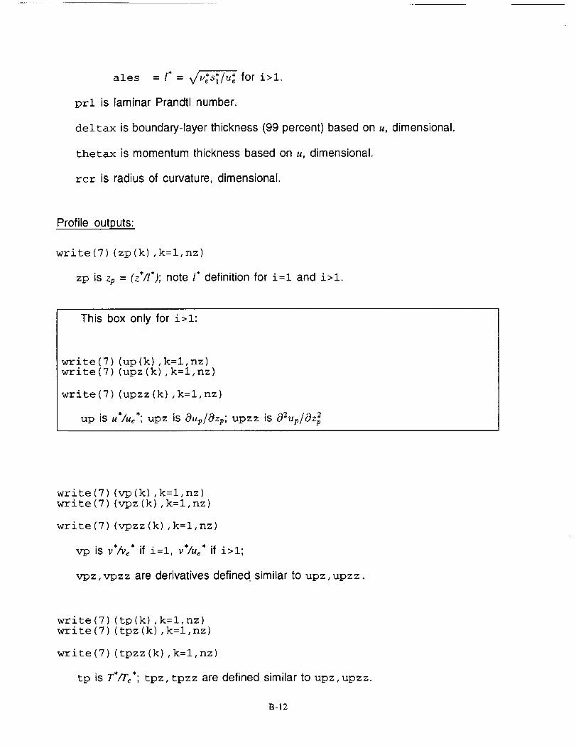
ales = 1" = _/yesl/u_ for i>l.
prl is laminar Prandtl number.
deltax is boundary-layer thickness (99 percent) based on u, dimensional.
thetax is momentum thickness based on u, dimensional.
rcr is radius of curvature, dimensional.
Profile outputs:
write(7) (zp(k),k=l,nz)
zp is zp = (z*/l*); note 1" definition for i=l and i>l.
This box only for i>1:
write(7) (up(k),k=l,nz)
write (7) (upz (k) ,k=l,nz)
write (7) (upzz (k) ,k=l, nz)
up is u*/.,*; upz is O%/Ozp; upzz is 02up/Oz 2
write(7) (vp(k),k=l,nz)
write(7) (vpz(k),k=l,nz)
write(7) (vpzz(k),k=l,nz)
Vp is 1}*lYe* if i=l, V*/Ue* if i>l;
_z,vpzz are derivatives defined similar to upz, upzz.
write(7) (tp(k),k:l,nz)
write(7) (tpz (k),k=l,nz)
write(7) (tpzz (k),k=l,nz)
tp is T*/Te*; tpz, tpzz are defined similar to upz, upzz.
B-12
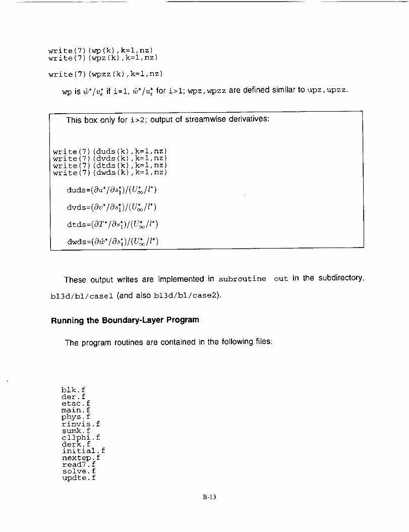
write(7) (wp(k),k=l,nz)
write(7) (wpz(k),k=l,nz)
write(7) (wpzz(k) ,k=l,nz)
wp is _*/v* if i=l, _*/u 2 for i>l; wpz, wpzz are defined similar to upz, upzz.
This box only for i>2; output of streamwise derivatives:
write(7) (duds(k) ,k=l,nz)write (7) (dvds (k) ,k=l, nz)
write(7) (dtds(k),k=l,nz)write (7) (dwds (k) ,k=l, nz)
duds=(a.*la, )l(U lt*)
/l*)
dtds=( OT* / cgS*l) / ( U_o/ l* )
These output writes are implemented in subroutine out in the subdirectory,
bl3d/bl/casel (and also bl3d/bl/case2).
Running the Boundary-Layer Program
The program routines are contained in the following files:
blk. fder. fetac. fmain. f
phys. frinvis, fsumk. f
cl3phi, fderk. finitial, f
nextep, fread7, fsolve, f
updte, f
B-13

conv. f
edge. finputs, fout. fref. fsum. f
In addition, the include files com and compack, the makefile makefile, and the
input file inp. dat are also provided. A brief description of important subroutines follows:
inputs, f. Reads input file inp.dat.
ref. f. Calculates reference quantities.
rinvis, f. Reads boundary-layer edge data bl.bin.
initial, f. Sets up initial profile at the attachment point i = l, j = ].
main. f. Calls various routines; specification of wall temperature or wall heat flux;
specifies wall suction rate.
edge. f. Specifies edge coefficients depending on boundary point or interior point;
calls cl3phi, f, etac. f to calculate some additional edge parameters.
etac. f. Sets up the y differencing coefficients based on the local crossflow direction
(L scheme or Z scheme).
blk. f. Sets up and solves the (7x7xnz) block tridiagonal system.
updte, f. Updates nonlinear quantities 0, 0', I, f, Ds, and l at k = ! for the current
iteration.
updte, f. Checks convergence.
phys. f. Outputs dimensional quantities, boundary-layer properties; calculates
crossflow.
nexstep, f: storing of variables prior to stepping in i.
out. f: output of quantities and profiles for boundary-layer stability analysis.
The include file corn has the following parameter statement (for casel in this
example):
B-14

par ame ter ( nx= 10 0, ny=2 9, nz = 61 )
The nx and ny values are as written out from the interface program. The value of
nz corresponds to the number of points in the boundary-layer normal direction.
The program is run with input files inp. dat and bl. bin. Appropriate dimensions
in parameter statement in the file corn are selected; then remove all . o files if com
was modified. Type make, followed by a. out to run the program. Runs can be made
interactively for moderate grids. The program execution stops at the (L ]) location where
the boundary layer separates; this results from the calculation of negative temperature
in subroutine update. An error message is printed out, and the incipient separation
condition can be checked by the local skin-friction coefficient.
B-15
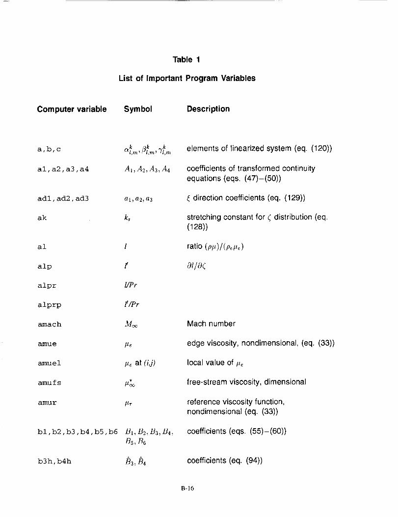
Computer variable
Table 1
List of Important Program Variables
Symbol Description
adl, ad2, ad3
ak
al
alp
alpr
alprp
amach
amu e
amuel
amufs
amur
bl,b2,b3,b4,b5,b6
b3h,b4h
a_m, _k k, l,m, _l,m
A1, A2, ,43, A4
al, a2, a3
k_
l
f
I/Pr
l'/Pr
Mc¢
#e
_e at (i,j)
/lr
B1, B2, B3, B4,
Bs, B6
B3: B4
elements of linearized system (eq. (120))
coefficients of transformed continuity
equations (eqs. (47)-(50))
,_ direction coefficients (eq. (129))
stretching constant for ( distribution (eq.
(128))
ratio (Pl_)/(P_#_)
o /o¢
Mach number
edge viscosity, nondimensional, (eq. (33))
local value of #_
free-stream viscosity, dimensional
reference viscosity function,nondimensional (eq. (33))
coefficients (eqs. (55)-(60))
coefficients (eq. (94))
B-16

Computer variable Symbol Description
b3t,b4t,b5t,b6t
bdl,bd2,bd3,bd4,
bd5
bet
bet2
ci,c2,c3,c4,c5,c6
c4h,c5h
c3t, c4t, c5t, c6t
c13
c132
cl3phix
cl3phiy
c24,c25,c26
c26x
c34,c35,c36
cbetal
cdl,cd2
chil,chi2,chi3
9'/(7-1)
(;- 1)/2
C1, C2, C3, C4,
Cs, C6
04,0
04,
Cl3
0132
(C13¢/hl),x
{ C13¢Yr / ( ]12tte) },y
C24, C2s, C26
£9C26/c9x
C34, C35, C36
_os (5),,j
l 12_ 12
XI_ X2, X3
coefficients (eq. (91))
7t direction differencing coefficients (eq.
(132))
coefficients (eqs. (62)-(67))
coefficients (eq. (95))
coefficients (eq. (92))
metric coefficient (eq. (6))
metric coefficient (eq. (48))
metric coefficient (eq. (50))
coefficients (eq. (19))
coefficient (eq. (80))
coefficients (eq. (20))
angle between grid lines (eq. (3))
constants (eq. (101))
coefficients (eq. (87))
B-17

Computer variable Symbol Description
dl,d2,d3,d4,d5
d5p
d3 t, d4 t
del fp, delgp,
delhp
delfpmax,
delgpmax,
delhpmax,
deltax
duds
el, e2, e3, e4
eps f, epsg, epsh
fl, f2
fe
fel
fey
fp
fpl, fp2
Dl, D2, D3, D4,
D5
ODs/O(
D3,D4
aSS, aS6, OS¢
max. of
0S5, aS6,0S7
F
(OuJOx)i=l
coefficients (eqs. (68)-(69))
coefficients (eq. (96))
solution vector elements (eq. (108))
convergence indicators
boundary-layer thickness based on F
reaching 99 percent value, dimensional
attachment-line velocity gradient
coefficients (eq. (87))
convergence criterion for change in
f',g', h' at wall (k = 1)
U/?Ae
F at i - 1 and i - 2
attachment-line velocity gradient
local value of fe
used in eq. (76)
a(_,l,_o)la(
ati-landi-2
B-18
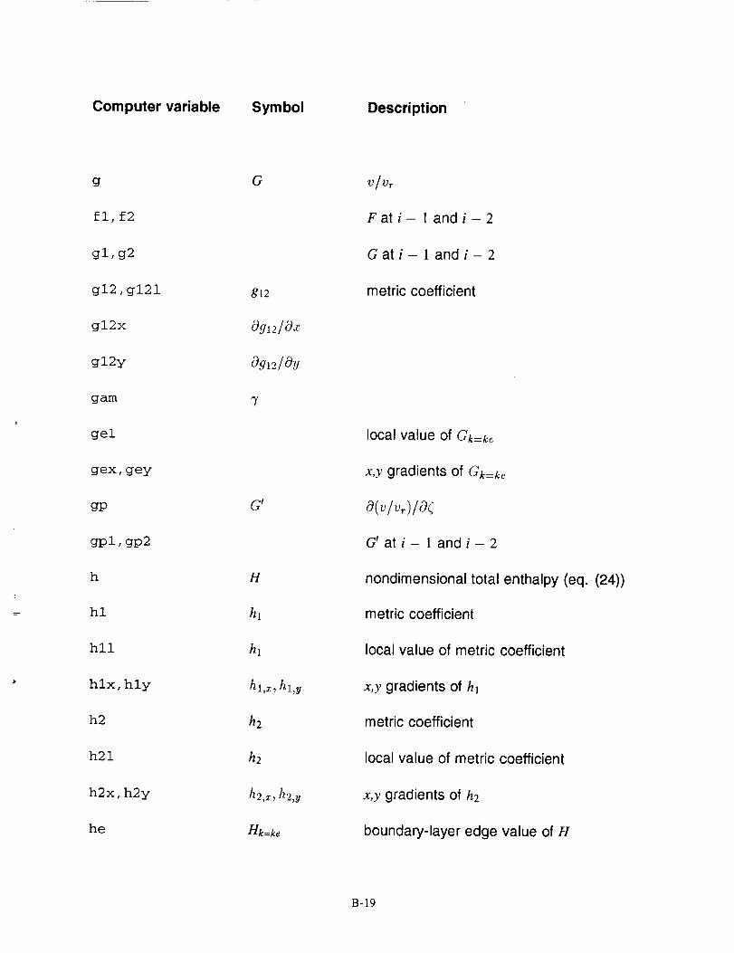
Computer variable Symbol Description
g
fl, f2
G
gl, g2
gl2,gl21 812
gl2x Og12/_gx
gl2y 09912/ogy
gam 7
gel
gex,gey
gP
gpl, gp2
h
hl
hll
hlx,hly
h2
h21
h2x,h2y
he
G I
H
hl
ha
hi,z, hl,y
h2
h2
h2,x, h2,y
Hk=ke
v/vr
F at i - 1 and i - 2
Gati- 1 and/- 2
metric coefficient
local value of Gk=ke
x,y gradients of Gk=k_
8(v lvr ) /cg¢
G rat/-land/-2
nondimensional total enthalpy (eq. (24))
metric coefficient
local value of metric coefficient
x,y gradients of hi
metric coefficient
local value of metric coefficient
x,y gradients of h2
boundary-layer edge value of H
B-19
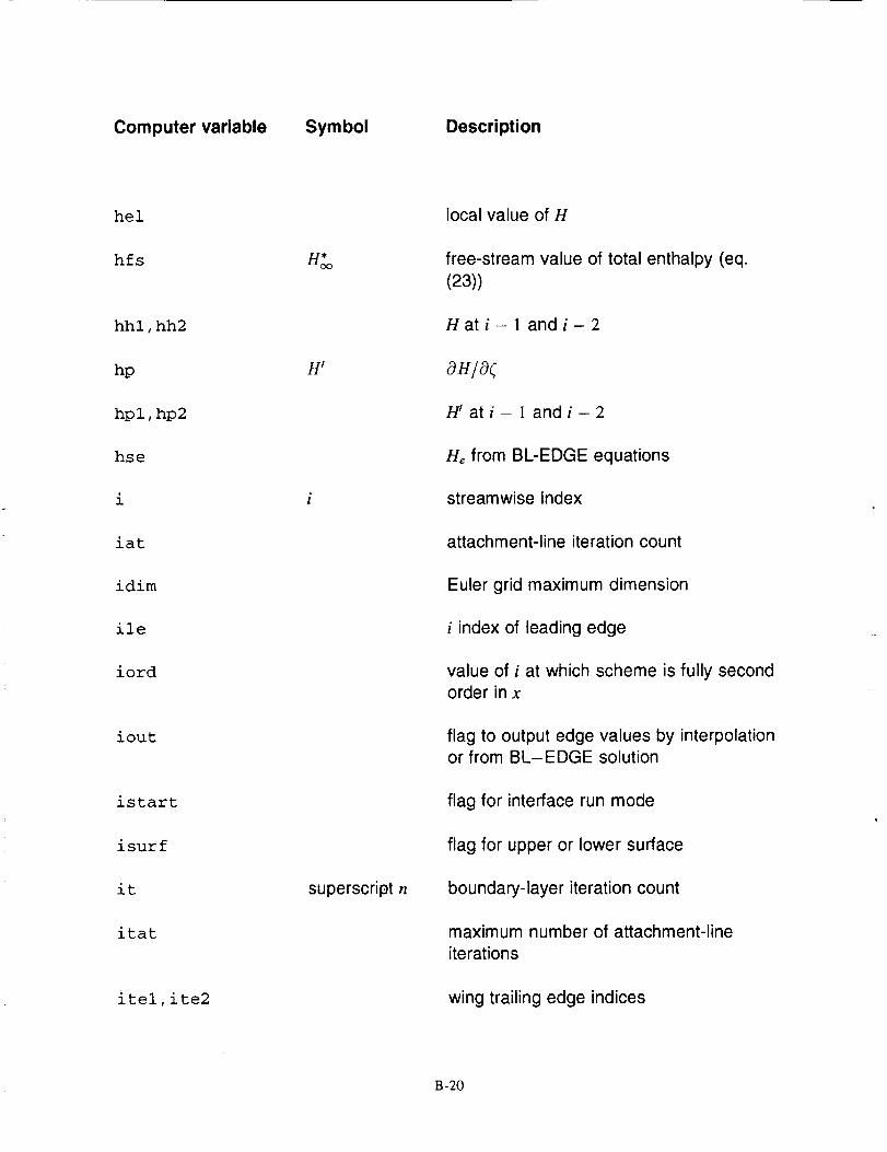
Computer variable Symbol Description
hel
hfs H i
hhl,hh2
hp H'
hpl, hp2
hse
i i
iat
idim
ile
iord
iout
istart
isurf
it
itat
itel,ite2
superscript n
local value of H
free-stream value of total enthalpy (eq.
(23))
Hati- landi-2
aHla
H'ati- ]andi-2
He from BL-EDGE equations
streamwise index
attachment-line iteration count
Euler grid maximum dimension
i index of leading edge
value of i at which scheme is fully secondorder in x
flag to output edge values by interpolationor from BL-EDGE solution
flag for interface run mode
flag for upper or lower surface
boundary-layer iteration count
maximum number of attachment-line
iterations
wing trailing edge indices
B-20

Computer variable Symbol Description
itmax
iunit
iv
ivm
iwall
J
jl,j2,j3,j4,j5
j lw, j2w
jdim
j tel, j te2
jv
jvm
kdim
i flagx
iflagy
maximum number of boundary-layeriterations
flag for U.S. units or S.I. units
number of points in streamwise direction,from interface run
maximum dimension for iv
flag for wall boundary condition
spanwise index
neighboring points of (i, j ) used in y
differencing
spanwise indices that correspond to
interface output
Euler grid maximum dimension
wing symmetry plane and tip indices
number of points in spanwise directionfrom interface run
maximum dimension for jv
Euler grid maximum dimension
flag to signify attachment-point solution orthree-dimensional solution
flag to signify LISW or generalthree-dimensional case
B-21
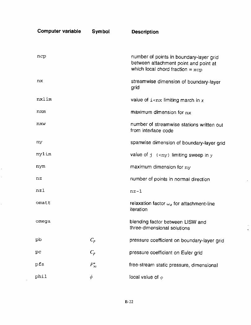
Computer variable Symbol Description
ncp
nx
nxlim
nxm
nxw
ny
nylim
nym
nz
nzl
omatt
omega
pb G
pc Cp
pfs
phil
number of points in boundary-layer gridbetween attachment point and point at
which local chord fraction = ×cp
streamwise dimension of boundary-layergrid
value of i<nx limiting march in x
maximum dimension for nx
number of streamwise stations written outfrom interface code
spanwise dimension of boundary-layer grid
value of j (<ny) limiting sweep in ),
maximum dimension for ny
number of points in normal direction
nz-I
relaxation factor _,, for attachment-lineiteration
blending factor between LISW andthree-dimensional solutions
pressure coefficient on boundary-layer grid
pressure coefficient on Euler grid
free-stream static pressure, dimensional
local value of _,
B-22

Computer variable Symbol Description
pi
prl Pr
q
qel
reflen
refls
refs
roe
roel
rofs
rstar
sll
tb
tC
re,tel
tfs
q
Re
Re
R*
$1
laminar Prandtl number
absolute velocity, nondimensional
local value of absolute edge velocity
reference length
free-stream Reynolds number based on
L_o (eq. (29))
free-stream Reynolds number per unit
length
boundary-layer edge density,nondimensional
local value of boundary-layer edge density
free-stream density, dimensional
gas constant
nondimensional arc length
nondimensional boundary-layer edge
temperature
nondimensional temperature from Eulersolution
nondimensional boundary-layer edge
tempe ratu re
free-stream dimensional temperature
B-23
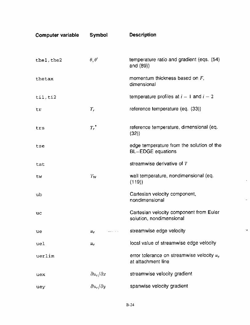
Computer variable Symbol Description
thel, the2 O, O'
thetax
til,ti2
tr Tr
temperature ratio and gradient (eqs. (54)and (89))
momentum thickness based on F,dimensional
temperature profiles at i - 1 and i - 2
reference temperature (eq. (33))
trs _*
tse
tst
tw TW
ub
uc
ue He
uel Ue
uerlim
uex
uey
reference temperature, dimensional (eq.
(32))
edge temperature from the solution of theBL-EDGE equations
streamwise derivative of T
wall temperature, nondimensional (eq.
(119))
Cartesian velocity component,nondimensional
Cartesian velocity component from Eulersolution, nondimensional
streamwise edge velocity
local value of streamwise edge velocity
error tolerance on streamwise velocity .eat attachment line
streamwise velocity gradient
spanwise velocity gradient
B-24
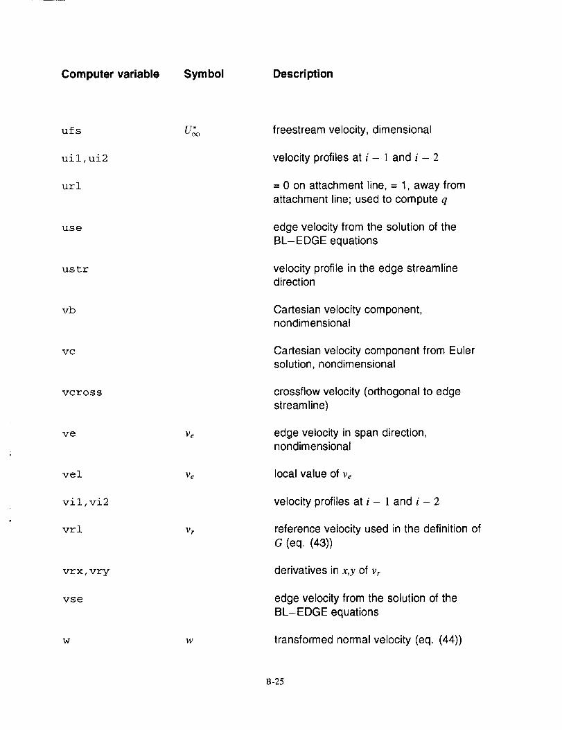
Computer variable Symbol Description
ufs U_o
uil,ui2
url
use
ustr
vb
vc
vcross
ve Ve
vel Ve
vil,vi2
vrl
vrx, vry
vse
Vr
w w
freestream velocity, dimensional
velocity profiles at i - 1 and i - 2
= 0 on attachment line, = 1, away from
attachment line; used to compute q
edge velocity from the solution of theBL-EDGE equations
velocity profile in the edge streamlinedirection
Cartesian velocity component,nondimensional
Cartesian velocity component from Eulersolution, nondimensional
crossflow velocity (orthogonal to edge
streamline)
edge velocity in span direction,nondimensional
local value of Ve
velocity profiles at i - 1 and i - 2
reference velocity used in the definition of
G (eq. (43))
derivatives in x,y of vr
edge velocity from the solution of theBL-EDGE equations
transformed normal velocity (eq. (44))
B-25

Computer variable Symbol Description
wb
wc
wil,wi2
x, y x,y
xb, yb, zb x'
xc,yc,zc
xcp
xnorm
z
zcon
zil,zi2
zphys
zphysx
zphysy
Z
Cartesian velocity component,nondimensional
Cartesian velocity component from Euler
solution, nondimensional
velocity profiles at i - ] and i - 2
streamwise boundary-layer coordinates
Cartesian coordinate of boundary-layer
grid
Cartesian coordinate of Euler grid
percent chord value at which ±=ncp
normalizing arc length, nondimensional
transformed boundary-layer normalcoordinate
coefficient to calculate zphys from z
zphys ati- l and i- 2
boundary-layer grid normal coordinate,dimensional
streamwise gradient of z
spanwise gradient of z
B-26
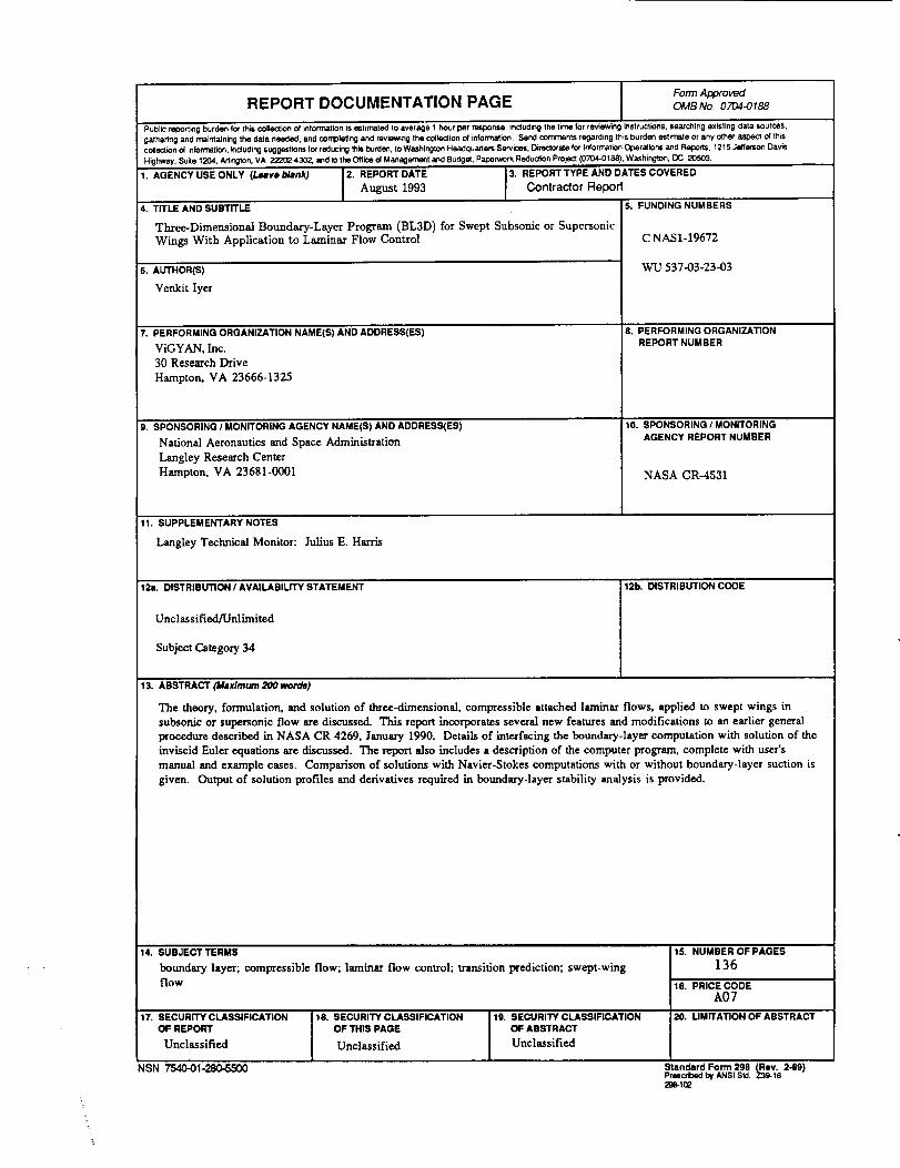
Form ApprovedREPORT DOCUMENTATION PAGE OMBNo 0704_188
Publlcreportingburdentot thiscollectionofInformationIs estimatedto average1hourperresponseincludingthe timeforreviewinginslruCliorts,sea'chin0 exislingdatasourCes,gatheflngand maintainingthe dataneededandcompletingandreviewingthecollectionofinformationSendcommentsregardingthisburdenestimateor ;anyotherespeclofthiscollectionol infornlatJen,includingsuggestloi_forreducingthis I:un:len,to WashingtonHeadquartersSe_,_oesDirestora_eforInformatio,nOpera_ionsandReports1215JeffersonOav_Hig_vay Suite1204,Arlington,VA 222024,302,endtotheOfficeof ManagementandBudge(,Paperv_rkReductbnProjen_(07D4_)188),Washington,CC 205_0
1 AGENCY USE ONLY (l.mave blank) 2 REPORT DATE 3 REPORT TYPE AND DATES COVERED
August 1993 Contractor Report
4 TITLE AND SUBTITLE 5 FUNDING NUMBERS
Three-Dimensional Boundary-Layer Program (BL3D) for Swept Subsonic or Supersonic
Wings With Application to Laminar Flow Control
6. AUTHOR(S)
VenY3t Iyer
7. PERFORMING ORGANIZATION NAME(B) AND ADDRESS(ES)
ViGYAN, Inc.
30 Research Drive
Hampton. VA 23666-1325
9. SPONSORING / MONITORING AGENCY NAME(S) AND ADDRESS(ES)
National Aeronautics and Space Administration
Langley Research Center
Hampton, VA 23681-0001
C NAS1-19672
WU 537-03-23-03
8. PERFORMING ORGANIZATIONREPORT NUMBER
10. SPONSORING/MONITORINGAGENCY REPORT NUMBER
NASA CR-4531
11. SUPPLEMENTARY NOTES
Langley Technical Monitor: Julius E. Harris
12a. DISTRIBUTION / AVAILABILITY STATEMENT 12b. DISTRIBUTION CODE
Unclassified/Unlimited
Subject Category 34
13. ABSTRACT (Maximum 200 word=)
The theory, formulation, and solution of three-dimensional, compressible attached laminar flows, applied to swept wings in
subsonic or supersonic flow are discussed. This report incorporates several new features and modifications to an earlier general
procedure described in NASA CR 4269, January 1990. DetaiLs of interfacing the boundary-Iayer computation with so]ution of the
inviscid Euler equations are discussed. The report also includes a description of the computer program, complete with user's
manual and example cases. Comparison of solutions with Navier-Stokes computations with or without boundary-layer suction is
given. Output of solution prof'des and derivatives required in boundary-layer stability analysis is provided.
14. SUBJECT TERMS
boundary layer; compressible flow; laminar flow control; transition prediction; sweptwing
flow
17. SECURITY CLASSIFICATIONOF REPORT
Unclassified
18. SECURITY CLASSIFICATIONOF THIS PAGE
Unclassified
NSN 7540-01-280-5500
15. NUMBER OF PAGES
136
18. PRICE CODEA07
19, SECURITY CLASSIFICATION 20. LIMITATION OF ABSTRACTOF ABSTRACT
Unclassified
Standard Form 298 (Rev_ 2-89)Prmcrbedby ANSIStd Z3_IO298tro