NUMERICAL SOLUTION OF STIFF ORDINARYDIFFERENTIAL EQUATIONS FORPOLYMERISATION KINETICS

At 63

D.A. JONES AND V. NANUT

MRL-TR-90-18

D Tl! C

AD-A238 181 JuLi , +jj,

MVATERIALS RESEARCH LABORATORYUDSll

Numerical Solution of StiffOrdinary Differential Equations

for Polymerisation Kinetics

D.A. Jones and V. Nanut ,%. e,4~

jus t If .C A t

MRL Technical Report itr~u~nM[RL-TR-90-18 Avrailabilty Codes~

IDIst Speoia1

Abstract W

This report describes the derivation of a set of ordinary differential equations tomodel radical chain polymnerisation. These equations have the mathematicalproperty of stiffness and are difficult to solve numerically. We show how theseequations can be solved efficiently ussing either the Gear or Kaps-Rentrop method.We also show how the kinetic scheme can be expanded to allow for the presence ofcontaminant scavenger molecules, aw. wVe apply these schemes to modelexperimental results for the polymeri, , don of N-vinyl-2-pyrrolidone obtained fromdilatometry measurements.

(*N-)

91-05156

DSTO 11110

MATERIALS RESEARCH LABORATORY

91 Y7 16 030

Published by

DSTO Materials Research LaboratoryCordite Avenue, MaribyrnongVictoria, 3032 Australia

Telephone: (03) 319 3887Fax: (03) 318 4536

© Commonwealth of Australia 1990AR No. 006-313

APPROVED FOR PUBLIC RELEASE

Authors

David Jones

David graduated from Monash University in 1972 witha BSc(Hons). He obtained his PhD from Monash in1976. His thesis was titled "Anisotropic diffusion inthe Townsend-Huxley experiment". After working atStrathclyde University, London University and theUniversity of Sydney he joined MRL in 1983.

Victor Nanut

Victor Nanut graduated BSc(Hons) in PhysicalChemistry from Monash University in 1981. Hejoined MRL in 1982 and for the first 3 years worked on

explosive devices, including their design and testing.He subsequently transferred to the explosiveformulation area where he has since worked on bothpressed and cast cured plastic bonded explosivecompositions.

L.

Contents

1. INTRODUCTION 7

2. KINETIC SCHEME FOR NVP POLYMERISATIONAND APPROXIMATE SOLUTIONS 8

3. NUMERICAL SOLUTION OF KINETICEQUATIONS 14

4. EXTENDED KINETIC SCHEME ANDNUMERICAL SOLUTION 20

5. CONCLUSION AND DISCUSSION 21

t 6. REFERENCES 22

Numerical Solution of StiffOrdinary Differential Equations

for Polymerisation Kinetics

1. Introduction

Materials Research Laboratory is currently engaged on a program of research anddevelopment on a number of cast-cured polymer bonded explosives (PBXs) as partof the the development of an Australian Insensitive Munitions capability. Thesefillings are formulated by dispersing solid explosive filler in a liquid pre-polymer,adding curing agent, mixing, then casting into the munition and curing in situ.Among the PBX formulations being studied is one which consists of RDX in anacrylic binder which is formed in situ by the copolymerisation of 2-ethylhexyl-acrylate (EHA), dioctylmaleate (DOM), and N-vinyl-2-pyrrolidone (NVP).

As part of a study of the curing of the binder in this PBX formulation aninvestigation of the mathematical modeling of the polymerisation reactions has alsostarted. The aim is to use the modeling as an aid to understanding the curingprocess and to have some predictive capability for cure rate as a function of variousparameters such as temperature, inhibitors, initiators and monomer ratios. We havebegun by considering the polymerisation of NVP in isolation from other bindermonomers and RDX. The polymerisation is initiated using 2,2'-azobis(2-methylpropionitrile) (AIBN) and the rate of the reaction is followed bydilatometry.

The mathematical model of this process is described by a set of coupled ordinarydifferential equations (ODEs) which have the mathematical property of stiffness,which means that the dependent variables can change on two or more very differentscales of the independent variable. This seriously complicates the numericalsolution of the coupled equations when simple explicit numerical schemes areemployed because the stability analysis shows that very small time steps must be

used even in regions where the solution is only slowly varying. For the NVPsystem this implies up to one million iterations of the solution procedure to followthe system for just one second.

Fortunately practical algorithms for the numerical solution of stiff ODEs havebeen devised and implemented in various software packages. A typical example isthe method due to Gear [1], which is implemented in the NAG routine D02EBF andis available at MRL [2]. The solution of these equations is so error prone, however,that it is both comforting and advisable to have a completely independent check ontheir accuracy. To provide such a practical and independent method of checkingthe solutions of our kinetic schemes we have implemented an efficient andrelatively simple algorithm for the numerical solution of stiff sets of ODEs. It isbased on the Kaps-Rentrop method [3] as described by Press and Teukolsky [4] anduses an implicit Runge-Kutta method. The algorithm requires no more than a fewhundred lines of FORTRAN coding and could easily be converted to BASIC andrun on a PC if so desired.

The purpose of this report is firstly to derive the equations which model theradical chain polymerisation process, and then to describe several numericaltechniques for the efficient solution of those equations. In the next section wedescribe the standard kinetic scheme for radical chain polymerisation of monomerssuch as NVP and then briefly discuss some approximate solutions of theseequations. In Section 3 we then describe several numerical methods for theirsolution. We have obtained solutions using an explicit 4th order Runge-Kuttaroutine, the NAG routine D02EBF based on the Gear method, and solutions usingthe Kaps-Rentrop method. Using the Kaps-Rentrop method we found excellentagreement with previous results, but with far less computational effort. To followthe model out to 8 000 seconds for example requires only 100 solution steps,whereas to check the results using the explicit Runge-Kutta code would haverequired approximately one billion steps. In Section 4 we extend the kineticscheme described in Section 2 to include the presence of radical scavengermolecules and illustrate the process of cure inhibition/retardation. We alsocompare the numerical solutions with experimental data on the polymerisation ofNVP contaminated with an as yet unidentified impurity.

2. Kinetic Scheme for NVP Polymerisationand Approximate Solutions

The polymerisation of NVP occurs by the radical chain mechanism. This scheme isdescribed in detail in standard texts [5, 61, and is briefly summarised here. Radicalpolymerisation is a chain reaction which requires the steps of initiation,propagation, and termination. The initiation step involves two reactions; first aninitiator I dissociates to form a pair of radicals R', and then in the second step aradical combines with a monomer molecule M to produce a chain initiating speciesM". These reactions are written as

S

I-. 2R' (1)

Re + M MI (2)

and occur with rate constants kd and ki respectively 1. In the propagation step thechain radical formed in the initiation step (M,') grows by the addition of very largenumbers of monomer molecules according to the general scheme

n successiveM I +M "---- M 2 " - Mn+2 " (3)

steps

The rate constant for propagation is denoted by kp and its numerical value isindependent of the size of the growing radical after the first few additions. The finalstep is the termination of polymer growth and this can occur in one of two ways,either combination or disproportionation. Both processes involve a bimolecularreaction of the radical sites at the ends of growing polymer molecules. Acombination reaction results in a single molecule, i.e. two ends have been joined bya chemical bond producing a larger chain. Disproportionation involves one radicalcentre gaining a proton resulting in one chain with a saturated chain termination andthe other with a double bond termination. Termination can also occur by acombination of coupling and disproportionation. The termination step is generallyrepresented by

Mn*+M* - M. (4)

where the particular mode of termination is not specified, and the rate constant kt isthe sum of the rate constants for each individual termination process.

Equations (1) through (4) can be described by the following set of coupled rateequations for the concentrations of initiator [I], radicals [R° ], monomers [M], andgrowing polymer molecules [M ].

dill- = - kd [I] (5)dt

1 The scheme depicted in equation (1) is nue only for a symmetical initiator L A more typical scheme is. follows

I --- RI* +R2 ° ,

with oily one i the decomposition producu beinS the ,macive species.

L

9

d[R"]dt = 2kdm- k,'[R 1 (6)dt

dM] =()-- ki [R ' -k [M ' IM (7)

d[M* I= _ 2R" [Me ]2 (8)

dt

Equation (5) indicates a simple exponential decay for the initiator concentration [I],and so the set of equations (5) through (8) can be replaced by the more convenientset

dRO- = 2fkdIo exp(-kdt)-kiReM (9)dt

dM- = -kiR M-kpMM' (10)dt

dM*- = kR"M-2kt(M) 2 (11)dt

where we have introduced the initiator efficiency f, which is defined as the fractionof the radicals produced in the decomposition reaction which initiate polymerchains. The value of f is usually less than one and we have used a value of 0.47,which was determined by Braun and Quella [7] for the initiation system being used.We have also dropped the bracket notation and simply let Re, M and Me denote theconcentrations of radical, monomer, and growing polymer molecules respectively.

The rate constants kd, ki, kp and k1 will determine the degree of stiffness of theset of equations (9) through (11). The rate of decomposition of the initiator kd(equation 1) can to a large degree be selected by choosing the appropriate chemicalsystem, and the rate of the overall polymerisation process can also be adjustedsubstantially by adjusting the concentration of the initiator and conditions to suit thepurpose of the polymer production process. For example, in a compilation ofdecomposition rate constants edited by Brundip and Immergut[81, kd varies over arange from 1010 s-' to 1071 st for various initiators under various conditions. Inthe case of the PBX the situation is complicated by the use of two peroxide initiatorsas well as cobalt (II) bisacetylacetonoate (CoAA). The CoAA allows the PBX tocure at room temperature because it facilitates the peroxide dissociation, i.e. kd isincreased by the presence of CoAA. We have not yet measured kd for theperoxides used in the PBX in the presence of CoAA, and for this study of the NVPpolymerisation a simpler initiation system using AIBN was chosen so thatcomparisons could be made with literature data. Braun and Quella[7] have

10

measured kd and found a value of 1.62 x 10-5 s-I at 60"C for AIBN. Ourexperiments have not yet yielded a value for kd.

The rate constants for the propagation step kP (equation 3) and the terminationstep 1 (equation 4) have been extensively studied for large numbers of monomers.Some of the data relevant to monomers in the PBX binder have been found in theliterature, but the relevant data is very limited. However it is known that for mostsystems the values of k and kt lie in the range 102 to 104 1 mole-1 s"1 and 106 to108 1 mole-' s-I respectively [6].

The rate constant ki for the initiation step (equation 2) is not known and rateconstants for reactions of this type have not been found in the literature. Howeverthe rates of reactions involving the so called "primary radicals" and the monomershould be of similar magnitude to the propagation rate constant kp (equation 3).This lack of knowledge regarding the value of ki is not critical as we will shortlydemonstrate that it has little effect on the overall rate of polymerisation.

With the above considerations in mind we have chosen to use the following setof values for the four rate constants for our preliminary investigation of the system:

kd = 1.6 x10 5 s"1

k. = 1.Ox 103 1 mole-1 s 1

kP= 1.0 X 103 1 mole

1 s1

kt 1.0 x W07t mole' s1

The range of values for the rate constants noted above means that the set ofequations (9) through (11) will have the mathematical property of stiffness.Technical definitions of stiffhess can be given in terms of the eigenvalues of theJacobian matrix formed from the equations [1], but here it simply suffices to notethat any set of equations in which the dependent variables can change on two ormore very different scales of the independent variable are called stiff. Stiff sets ofequations are notoriously difficult to solve numerically using explicit schemesbecause the stability of the scheme is governed by the size of the time step neededto resolve details of changes occurring on the fastest time scale. This means thatvery small time steps are required to follow changes over very much longer periodsof time, even though the solutions may not be varying rapidly on this time scale.Before describing a practical method for overcoming this problem in the nextsection, we first briefly describe an approximate solution of the equations (9)through (11) to get a feel for their behaviour.

The analysis of radical chain polymerisation in most textbooks begins byassuming the steady state condition, i.e. the assumpton is made that the rate ofinitiation is equal to the rate of termination, so that the concentration of free radicalsbecomes essentially constant very early in the reaction. We use this assumptionourselves in a moment, but first note that the decrease in monomer concentration

11

during a typical polymerisation of the type involved in our PBX binder studies isvery slow, decreasing by approximately 10% over a time of several hours. Thismeans that we can replace the variable M in equation (9) by its initial value Mo at tequals ze'o. Also, the value of kd is such that the exponential in equation (9) maybe replaced by unity for times shorter than one hour. Equation (9) then becomes

dR"- f= 2 fkdlo - ki MOR* (12)

dt

with solution

Re (t) =ffi- ( 1- exp (- ki Mot)) (13)k. Mo

indicating a rise to a steady state value of 2fkdIO/kiMO in a time of order (kiMo)'l.Appropriate experimental values for Mo and 10 are 9.08 moles 1- and 1.52 x 10-3

moles 1i respectively and these lead to a steady state value of Re = 2.5 x 1012moles 11 in a time of about 10-4 s.

We now set dM* /dt equal to zero in equation (11) and assume that the radicalconcentration has reached its equilibrium value R* . We then obtain the followingexpression for the equilibrium value of M

me = [ Rq Mo (14)2k,

Using the values for the constants given above this leads to a value ofMe = 3.4 x 108 mole 1-. We could solve equation (11) exactly to obtain anestin~ate of the time taken for M* to reach this equilibrium value by substituting thesolution for R" given by equation (13) into equation (11). The resulting equationis a Riccati equation, which is not easy to solve, but solutions can be expressed interms of the solutions of two auxiliary equations (9]. We have not pursued thisapproach however as we know from prior experience that this time scale is on theorder of seconds or less.

We now consider the decrease in monomer concentration on the slower timescale. Assuming that both R° and Me do not vary greatly from their equilibriumvalues as M begins to decrease, we can treat equation (10) as a simple equation inthe single variable M. The solution is then

M(t) f Mo exp (- kt) (15)

where

k z-R'eq+k' MOeq (16)

12

With the values forkk R ° and M' used above k can be approximated veryclosely by kpM9 . and tie exponential cn be expanded to first order to give

M(t) = Mo (1 - kp [(kd/k) f I] 1 2 t, (17)

indicating that a plot of monomer concentration versus time for the early stage ofmonomer consumption should lie on a straight line and have a negative gradient ofMo kp {(kd/kt) f 10 112. That this is indeed the case can be seen in Figure 1, whichshows a relationship between monomer concentration and time, derived fromexperimental data obtained with a dilatometer during an NVP polymerisationreaction. The monomer concentration versus time data was obtained from thevolume change versus time data by using a conversion factor which incorporates thedensities of NVP and the polymer at the temperature of the reaction. Thisconversion factor is only known at 20C at present and this value was used eventhough the data was obtained at 60"C. The data cannot therefore yet be used toobtain accurate values of kinetic parameters, but it can be used to provide acomparison for the model output and approximate values of parameters.

- 9.0

7.5

-500 0 500 1000 1500 2000 2500

Time. s

Figure): Experimental data for monomer concentration versus time for NVP.

Given that kd, f, I and Mo are known, a value for the ratio k_2/k, can be obtainedfrom the straight line fit to the experimental data in Figure 1. In practise, a moreaccurate method u± doing this is to obtain the gradient dM/dt for several values ofthe initial initiator concentration Io . From equation (17) we easily have

- dM/dt = [Mo(fkd 1/2 (k 1̂)l/2 ] 101/2 (18)

13

and so a plot of gradient versus Ioli2 again leads to a value of kP2/k. Measurementsof kp2/k as a function of temperature lead to useful information about thethermochemistry of polymerisation, but it is importani to note that values for kP and1 separately can only be obtained by non steady-state methods [5]. We at,currently reviewing the need to use a non-steady-state method such as the rotatingsector method [6] to obtain the additional experimental data required to separate kpandk,.

Equation (17) also indicates that, with the range of values for the rate constantswe are using, the initial rate of polymerisation is effectively independent of the rateconstant ki and justifies our assertion that knowledge of an exact value for ki is notrequired for the polymerisation experiments we are planning.

3. Numerical Solution of Kinetic Equations

The initial rapid rise of Re to its equilibrium value Re on a time scale of theorder of milliseconds is easily demonstrated using a simpe 4th order Runge-Kuttaintegration routine. Figures 2 and 3 show solutions of equations (9) through (11)obtained using the program RKUTTA. (The source code for the programsreferred to in this report arc available from the authors). The rate constants kd, ki,kp, kt and the initial constants M0 and 10 were set to the values used in the previoussection. Figure 2 was calculated using a time step At of 1 pts and shows that Rereaches an equilibrium value of 2.5 x 10-12 mole 1- in a time of approximately0.5 ms, which is in good agreement with the approximate calculation in the previoussection. On this time scale M remains constant while M" increases linearly withtime, as can be seen in Figure 3, which shows both Re and M" between t = 0 and5.0 ms calculated using a time step of 5.0 pts.

To use the program RKUTIA to follow the time variation of either M ° or Mwould be completely impractical. A time step of the order of 10 pts would beneeded to establish the equilibrium value of Re accurately, and then many millionsof steps would be needed to track either Me or M. The sensible procedure tofollow for the solution of stiff sets of equations such as (9) through (11) is to useone of the software packages specifically designed for the solution of theseequations. These are usually based on implicit schemes with variable step lengthand automatic local error control. A particularly well known procedure for thesolution of stiff sets of equations is the Gear method [I], which is available at MRLas subroutine D02EBF of the NAG group of software packages. We have used theGear method to follow the full time dependence of the variables in equations (9)through (11).

14

24

20r

x 16

1 2U

0 0.2 0.4 0.6 0.5 1.0

lIme. ms

Figure 2: Radical concentration versus time calculated from program RKUTTAwith At =I Ws.

12

10

E

x

e 6

_2

ii 4

2 Rx 0

0 1 2 3 '.

71me. ms

Figure 3: Concenrations of radials and growing polymer molecules calculatedfrom program RKUTTA with At = 5.0 .

1s

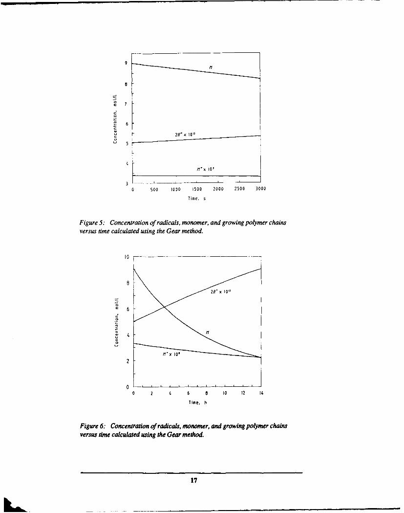
Figure 4 shows the time dependence of M° on a time scale of seconds. We see thatM' approaches a steady state value of 3.4 x 10-8 moles 1-1, which is again in goodagreement with the approximate solution in the previous section. Figure 5 showsR° ,M" and Mover a longer time scale. We see that both R and M vary littlefrom their equilibrium values, justifying the assumption made in the previoussection, and that over this time scale M decreases linearly with time, again inagreement with the analysis in the previous section. To display the exponential timedependence of M requires following the solution over a much longer time scale.We have done this and show the solutions in Figure 6. The exponential decay of Mis now clearly evident.

32

28

S 2'4E

x 20

Z 16

12

I.00

0 7 4. 6 8 10

Time. s

Figure 4: Concentration of growing polymer molecules versus time calculatedusing the Gear method.

We have used the subroutine DO2EBF to check some of the assumptions andconclusions of the previous section. In particular, our analysis predicts that over atime scale of just a few hours M should decrease linearly with time, and that thegradient of this time should be independent of ki , and depend on k and kt only inthe ratio k 2/k. We have checked these results by varying k. over the range I x 102

to I x 104 and found that it has had no effect on the time dependence of M over thetime scale of interest. We have also varied the values of kp and k, and again foundthat the time dependence of M is unaltered if the value of the ratio kp2Ikt remainsconstant.

16

LI _ _

9

7

6

U 2R'x 10 I

-, 5

flx 10'

0 500 1000 1500 2000 2500 3000

Time. s

Figure 5: Concentration of radicals, monomer, and growing polymer chainsversus time calculated using the Gear method.

8 I 2R" x 10,"

6

dH4

C

0 2 1 6 8 to 12 14

Time. h

Figure 6: Concentration of radicals, monomer, and growing polymer chainsversus time calculated using the Gear method.

17

The Gear method, as implemented in D02EBF, is both simple and efficient to use,and capable of providing solutions to any desired degree of accuracy by setting anappropriate value of the parameter TOL in the calling sequence. It is however a"black box", and on the few occasions when the method has failed it has not beeneasy to trace the underlying cause of this failure. To overcome this problem, andalso to provide a completely independent means of checking the accuracy of thesolutions produced by D02EBF, we have recently implemented a new method forthe solution of stiff sets of equations. The method is due to Kaps and Rentrop [3],and the implementation described here was devised by Press and Teukolsky [4].

A set of non-linear ODEs can be written in the form

y, = f(y) (19)

where y is the vector (yl, y2 ...... yN) of N dependent variables, and the primedenotes differentiation with respect to time. The Kaps-Rentrop method seeks asolution of the form

S

y(to+h) =y+ EC ki (20)

where the corrections ki are found by solving s linear equations of the form

i-I(1- Tif )-k = hf (y0

+ E o,., k)

i-I j=1+ hf'. -E ij j if =1.....s. (21)

Here the coefficients y, C., m. and y. are fixed constants independent of the

problem. Automatic step size adjustment is provided using theRunge-Kutta-Fehlberg method [4]; two estimates having the form of equation (20)are computed, one of higher order than the other, the difference between the twothen leads to an estimate of the local truncation error, which can then be used forstep size control. Control of the local step size error can be maintained by asuitable choice of the parameter EPS in the calling progrmn.

Tables I through 3 illustrate the degree of accuracy obtainable using both theGear and Kaps-Rentrop methods. It should be noted that the Gear method isimplemented in double precision, while the Kaps-Rentrop method uses only singleprecision. The KAPS program is marginally faster than the GEAR program, butboth take no more than a few seconds of CPU time.

18

Table 1: Gear Method : TOL = 104

t(s) Re x 1012 M Me x 101

500 2.5364 8.9412 3.36801000 2.5587 8.7939 3.35402000 2.6032 8.5048 3.37893000 2.6484 8.2274 3.30074000 2.6935 7.9612 3.2744

Table 2: Gear Method: TOL = 1010

t(s) Re x 1012 M Me x 101

500 2.5401 8.9284 3.36741000 2.5625 8.7796 3.35402000 2.6075 8.4911 3.32723000 2.6526 8.2143 3.30074000 2.6978 7.9487 3.2744

Table 3: Kaps-Rentrop Method: EPS = 10-

t(s) R° x 1012 M Me x 108

500 2.5432 8.9284 3.36891000 2.5676 8.7796 3.35682000 2.6113 8.4911 2,.32913000 2.6578 8.2143 3.30354000 2.7021 7.9457 3.2766

19

4. Extended Kinetic Scheme and Numerical Solution

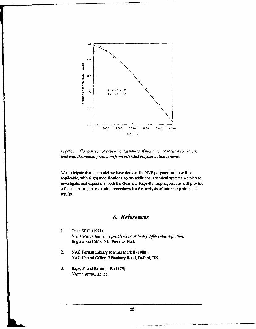
The analysis presented in Section 2 for radical chain polymerisation using typicalvalues for the rate constants kd, k P, k and the initial constants Io and Mo clearlyshows that the monomer concentration will decay linearly with time for times lessthan one or two hours. Slight variations in some of the values of these constantswill not change this general picture, the slope of the line may change, but thedecrease will still be linear with time. Figure 7 shows some experimental points forNVP monomer concentration versus time which were obtained dilatometrically inthe same manner as described in Section 2. The only significant difference in theexperimental procedure was that a different batch of NVP was used. Thepronounced downward concavity of these points indicates that some mechanismother than simple radical chain polymerisation must be operating.

To explain these results we have assumed the existence of a contaminantscavenger molecule which removes both radicals and activated monomer. We caninclude the presence of such a contaminant by slightly expanding the kinetic schemeoutlined in section 2. We define a scavenger concentration [S" ] which acts on both[R° ] and [M° ] as follows

Re +So - RS (22)

M" +S" - MS (23)

Formation of the molecular species RS and MS removes both Re and M° fromactive participation in the radical chain growth process. We assume rate constantski and k2 for equations (22) and (23) respectively. Equations (22) and (23) cannow be included in an expanded kinetic scheme which has the following form

d[I]- - kd [] (24)

dt

d[R"]-- = 2kd []- kR ]I[M]- k, [R )[S°] (25)dt

d[MJ= - ki [R ][M]- kp [MJ ][M] (26)dt

d[M" I- = k [R" )[KI- 2kt [Me ]2 - k2 (Me ][So 1 (27)

dtd[S" I = -k, LR* ](So k2 [Me ]IS. ) (28)

20

We again simplify this set of equations by incorporating the exponential solution ofequation (24) and dropping the bracket notation. The equations then become

dRe- = 2 fkdIoexp(-kdt)-ki R"M-k RS (29)dt1

dM- = -k i1RM-kp MM (30)dt

dM*- = kiR"M-2kt(Me)2- k2 me so (31)dt

dS*- = -k1 ROS -k 2 (M*S*) (32)dt

We have solved the set of equations (29) through (32) using both the NAG routineD02EBF and the Kaps-Rentrop method and found the results to be identical withinthe error tolerances of both schemes. We have no knowledge of the values of k,and k2 so we have simply set k, = k2 = k, and used k as a parameter to be varieduntil agreement can be found with the experimental results. The curve shown inFigure 7 was calculated using k = 5.0 x W, with the other constants having theirprevious values. The good agreement with experiment indicates that ourassumption of the presence of a contaminant scavenger molecule appears to becorrect.

5. Conclusion and Discussion

This report has described our analysis of the kinetics of the polymerisation of NVP.We have discussed the kinetic scheme appropriate to radical chain polymerisationand derived appropriate equations to model this system. We have shown how toobtain approximate solutions to these equations, and also discussed appropriatenumerical algorithms for the efficient solution of these equations. Our analysis hasshown that by following the polymerisation rate using dilatometry methods we canobtain a value for the ratio kp2/k1 , but that further experimental information isrequired to obtain values for k and k1 separately. We are currently evaluating thefeasibility of several experimental techniques to provide this information.

We have applied the mathematical model to some preliminary experiments onNVP polymerisation and found good agreement between the model and theexperimental results. We plan to expand the experimental part of this programconsiderably, the objective being to determine the kinetic parameters necessary tomodel a terpolymerisation involving the three monomers NVP, EHA and DOM. Inaddition we wish to study the effects of inhibitors (radical scavanger molecules).

21

9.1

8.9

E 8.7

'U

8.3

0 1000 2000 3000 4000 5000 6000

Time. s

Figure 7: Comparison of experimental values of monomer concentration versustime with theoretical prediction from extended polymerization scheme.

We anticipate that the model we have derived for NVP polymerisation will beapplicable, with slight modifications, to the additional chemical systems we plan toinvestigate, and expect that both the Gear and Kaps-Rentrop algorithms will provideefficient and accurate solution procedures for the analysis of future experimentalresults.

6. References

1. Gear, W.C. (1971).Numerical initial value problems in ordinary differential equations.Englewood Cliffs, NJ: Prentice-Hall.

2. NAG Fortran Library Manual Mark 8 (1980).NAG Central Office, 7 Banbury Road, Oxford, UK.

3. Kaps, P. and Rentrop, P. (1979).Numer. Math., 33, 55.

22

4. Press, W.I1. and Teukoisky, S.A. (1989).Integrating stiff ordinary differential equations. Computers in Physics,88-91, May/June 1989.

5. Billmeyer, F.W. Jr., (1971).Textbook of polymer science, Second Edition. New York: John Wiley and

Sons.

6. Odian, 0. (1970).Principles of polymerization. New York: McGraw-Hill Book Company.

7. Braun, D. and Quella, F. (1978).Macromol. Chem., 179, 387-394.

8. Brundup, J. and Imniergut, E.H. (eds) (1966).Polymer handbook. New York: Interscience Publishers, John Wiley & SonsInc.

9. Gradshteyn, 1.S. and Ryzhik, I.M. (1980).Tables of integrals, series and products. Academic Press.

23

SECURITY CLASSIFCATION OF THIS PAGE UNCLASSIFIED

DOCUMENT CONTROL DATA SHEET

REPORT NO. AR NO. REPORT SECURITY CLASSIFICATION

MRL-TR-90-18 AR-006-3t 3 Unclassified

TITLE

Numerical solution of stiff ordinary differentialequations for polymerisation kinetics

AUTHOR(S) CORPORATE AUTHOR

DSTO Materials Research LaboratoryD.A. Jones and V. Nanut PO Box 50

Ascot Vale Victoria 3032

REPORT DATE TASK NO. SPONSORDecember, 1990 87/156 RAAF

FILE NO. REFERENCES PAGESG6/4/8-3912 9 24

CLASSIFICATION/IIM1TATION REVIEW DATE CLASSIFICATION/RELEASE AUTHORITYChief, Explosives Division

SECONDARY DISTRIBUTION

Approved for public release

ANNOUNCEMENT

Announcement of this report is unlimited

KEYWORDS

Polymerisation KineticsStiff Ordinary Differential Equations

SUBJECT GROUPS

ABSTRACT

This report describes the derivation of a set of ordinary differential equations to model radical chain polymerisation.These equations have the mathematical property of stiffness and are difficult to solve numerically. We show how theseequations can be solved efficiently using either the Gear or Kaps-Rentrop method. We also show how the kinetic schemecan be expanded to allow for the presence of contaminant scavenger molecules, and we apply these schemes to modelexperimental results for the polymerisation of N-vinyl-2-pyrrolidone obtained from dilatometry measurements.

SECURITY CLASSIFCATION OF THIS PAGEUNCLASSIFIED