Embed Size (px)
Citation preview

MPRAMunich Personal RePEc Archive
KANBAN system in AutomobileIndustries: Feasible Study
Ammar Aldubaikhi
Lamar University
13. June 2014
Online at https://mpra.ub.uni-muenchen.de/66942/MPRA Paper No. 66942, posted 28. September 2015 17:57 UTC

1
KANBAN system in Automobile Industries: Feasible Study
Ammar Aldubaikhi
Doctorate Researcher in Industrial Engineering
Lamar University
2
Abstract
The current running company uses MRP system for production and inventory. The main
client decided to change its ordering system to KANBAN JIT. Hence company should
make decision either keep pervious system (MRP) or follow client and move to KANBAN
JIT. The following report addresses the change to JIT and provide conclusion to the
decision maker.
3
1. Introduction
Company which project has done located in Saudi Arabia. It started producing Auto
parts since ten years ago when economical stimulations were given by government to
produce inside country. The company produces more than eighteen group products,
which include either one or more in each group. Electronic and Mechatronic are two main
areas that company work on it.
Main client orders more than 95 percent of company product. The reason of that
company count on one client is monopoly of products and only company that located in
level one of client grading. Client has a grading system for its supplier, based on this
system each supplier twice a year has audit by client in whole company area such as
financial, production, supply chain, purchasing and after sell services. After audit each
company based on grade that obtained divided in three levels. Level one company
achieve 80 percent of client order, level two obtain 15 percent of order and level three get
last 5 percent.
The company uses MRP system for production and inventory. Client decided to
change its ordering system to KANBAN JIT. Hence company should make decision either
keep pervious system (MRP) or follow client and move to KANBAN JIT.
2.1 Problem Statement:
Change in client ordering system that affects all suppliers responding. The decision
should be to react to this change based on the capabilities and current situation in
company.
2.2 Scenarios to deal with new change:
1-‐‑ Follow same way as client to run KANBAN JIT system in company.
2-‐‑ Keep MRP system and adjust based on new situation.
2.3 Goal of this project:
4
This project seeks to select one of the above two scenarios based on comparing them
in all cost related on them. Moreover, after choosing the most appropriate one draw
roadmap to obtain maximum efficiency.
3. Methodology:
First, negotiate with suppliers based on new ordering process and suppliers divide to
two groups, follower, and not follower. Then Follower suppliers define their lead-‐‑
time. KANBAN cards define based on new lead-‐‑time for follower. The suppliers who
could not follow new system EOQ method use to order.
1-‐‑ Predict demand for items that provide by suppliers who could not follow
KANABAN system.
2-‐‑ Designing the KANBAN system.
4. Forecasting the demand
Data and Analysis
4.1 Data
4.1.1 Historical Data
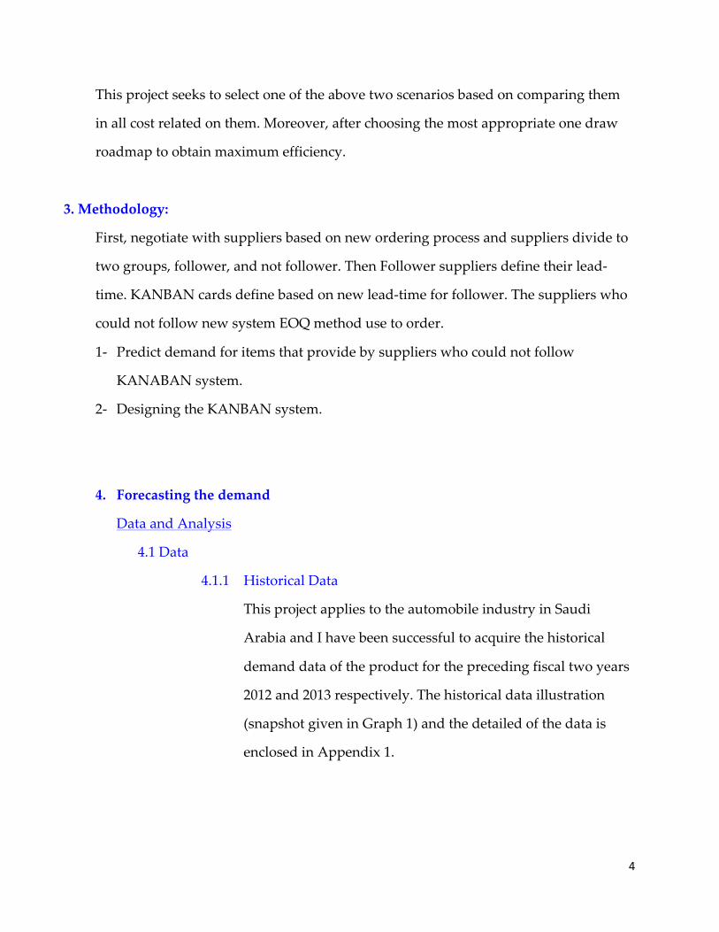
This project applies to the automobile industry in Saudi
Arabia and I have been successful to acquire the historical
demand data of the product for the preceding fiscal two years
2012 and 2013 respectively. The historical data illustration
(snapshot given in Graph 1) and the detailed of the data is
enclosed in Appendix 1.
5
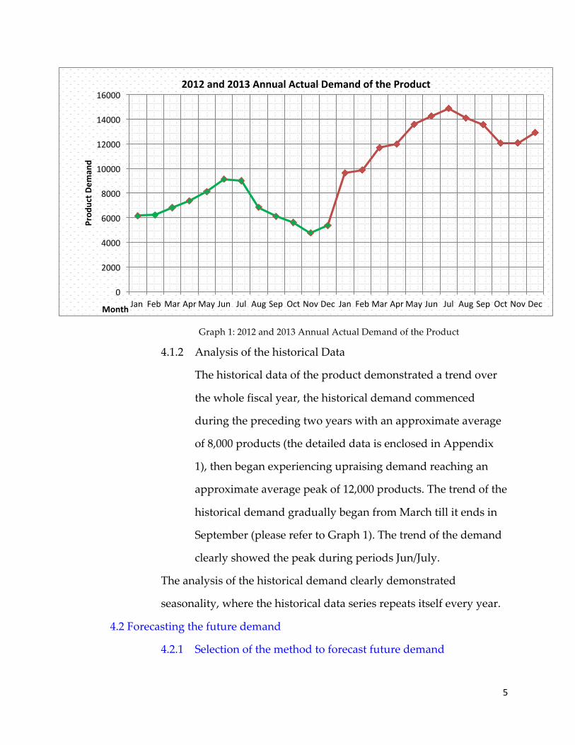
Graph 1: 2012 and 2013 Annual Actual Demand of the Product
4.1.2 Analysis of the historical Data
The historical data of the product demonstrated a trend over
the whole fiscal year, the historical demand commenced
during the preceding two years with an approximate average
of 8,000 products (the detailed data is enclosed in Appendix
1), then began experiencing upraising demand reaching an
approximate average peak of 12,000 products. The trend of the
historical demand gradually began from March till it ends in
September (please refer to Graph 1). The trend of the demand
clearly showed the peak during periods Jun/July.
The analysis of the historical demand clearly demonstrated
seasonality, where the historical data series repeats itself every year.
4.2 Forecasting the future demand
4.2.1 Selection of the method to forecast future demand
0
2000
4000
6000
8000
10000
12000
14000
16000
Jan Feb Mar Apr May Jun Jul Aug Sep Oct Nov Dec Jan Feb Mar Apr May Jun Jul Aug Sep Oct Nov Dec
Prod
uct D
eman
d
Month
2012 and 2013 Annual Actual Demand of the Product
6
In order to proceed with forecast of the future demand, first
the quest was to find a forecasting model that incorporate the
product trend in the market. Doing so, the forecasted figures
will realistically reflect the market situation and will keep the
reliability of the output data. The model chosen to forecast
future demand was the Seasonal Factors for Stationary Series.
4.2.2 The method of forecasting
The seasonal Factors for Stationary Series method is a simple
method of computing the seasonal factors for a time series
with Seasonal variation and trend (Nahmias, 2008). The
method requires minimum of two seasons of data, which I
have the historical demand for 2012 and 2013.
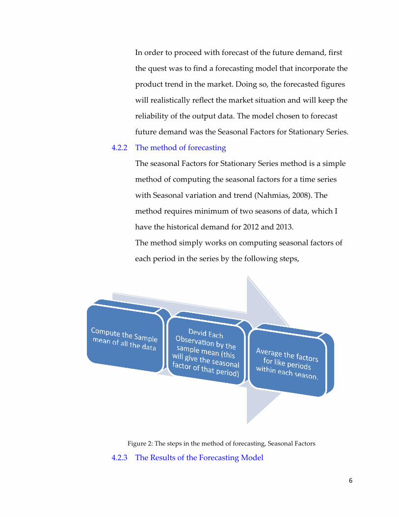
The method simply works on computing seasonal factors of
each period in the series by the following steps,
Figure 2: The steps in the method of forecasting, Seasonal Factors
4.2.3 The Results of the Forecasting Model
7
Now, applying this method to the set of the historical demand
that I have, resulted in sample mean of all observation equals
to (12833 products), then the Seasonal Factors of each period
(month) of the last two years are 0.65, 0.65, 0.72, 0.78, 0.85,
0.86, 0.95, 0.72, 0.64, 0.59, 0.50, 0.56, 0.99, 1.01, 1.20, 1.23, 1.39,
1.46, 1.52, 1.44, 1.39, 1.24, 1.24 and 1.32. These factors represent
the months starting from January and ending in December.
Now we average the factors for like periods, for example the
seasonal factor for January 2012 is 0.65 and the one for January
2013 is 0.99; the resulted average seasonal factor for the period
(January) equals to 0.82. Applying this to all the periods gives
the following average seasonal factors (0.82, 0.83, 0.96, 1.00,
1.12, 1.21, 1.24, 1.08, 1.02, 0.91, 0.87 and 0.94.
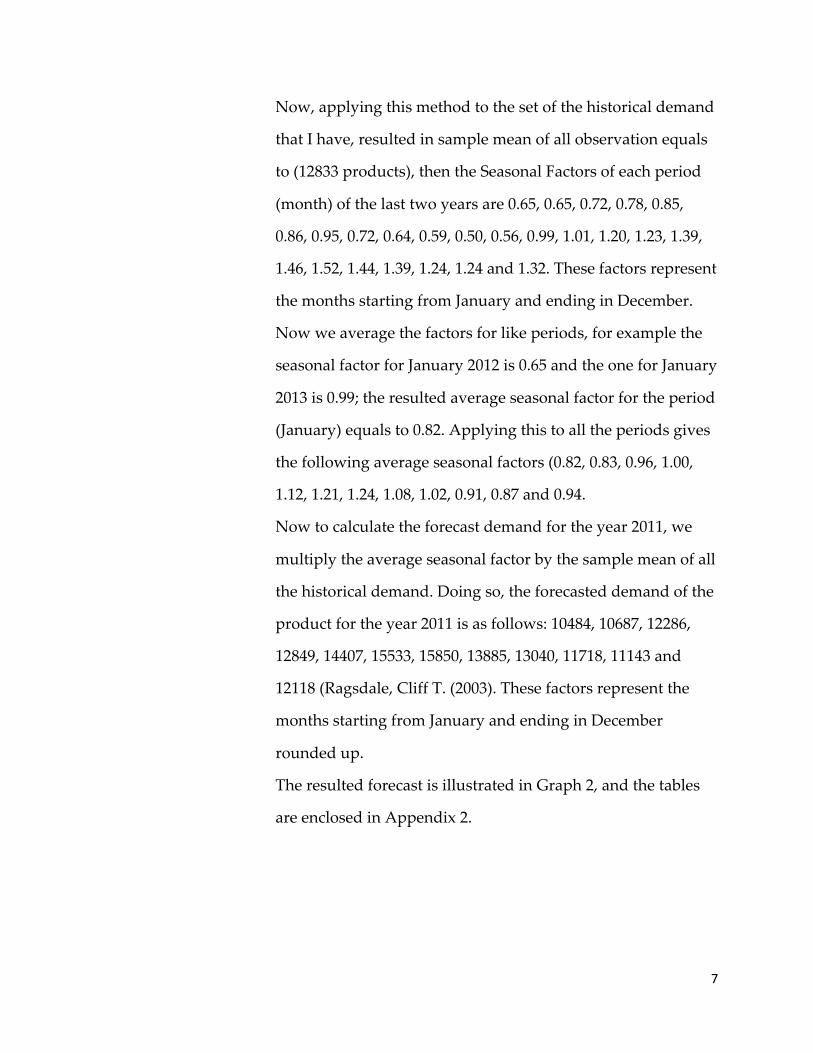
Now to calculate the forecast demand for the year 2011, we
multiply the average seasonal factor by the sample mean of all
the historical demand. Doing so, the forecasted demand of the
product for the year 2011 is as follows: 10484, 10687, 12286,
12849, 14407, 15533, 15850, 13885, 13040, 11718, 11143 and
12118 (Ragsdale, Cliff T. (2003). These factors represent the
months starting from January and ending in December
rounded up.
The resulted forecast is illustrated in Graph 2, and the tables
are enclosed in Appendix 2.
8
Graph 2: Future demand forecast
4.3 Validation and substantiation
In order to validate the forecasted data using the seasonal Factors for
Stationary Series methods, I have consulted the output of the method with
the factory engineer. The feedback on the data and the forecast analysis was
adequate and represent the real situation.
5. Designing KANBAN system
Assumptions:
1-‐‑ One product chooses as a prototype for this project.
2-‐‑ Client send its order once a day by predefine quantity (no more than one
KANBAN).
3-‐‑ All suppliers could not follow KANBAN either they have minimum quantity
order or long lead time.
4-‐‑ Suppliers who could not follow KANBAN, we keep ordering based on EOQ and
storages are known as another supplier in KANBAN system with zero lead time.
0
2000
4000
6000
8000
10000
12000
14000
16000
18000
Jan Feb Mar Apr May Jun Jul Aug Sep Oct Nov Dec
Deman
d Forecaste
Month
2014 Demand Forecaste
9
5-‐‑ The scope of KANBAN for this project is suppliers and fellow KANBAN cards
between suppliers and manufacturing (manufacturing already has set up for
KANBAN).
6-‐‑ Single card is selected for this project because just suppliers are in scope, so
KANBAN card for production automatically omitted and just use replenishment
card (SAP AG and KANBAN website).
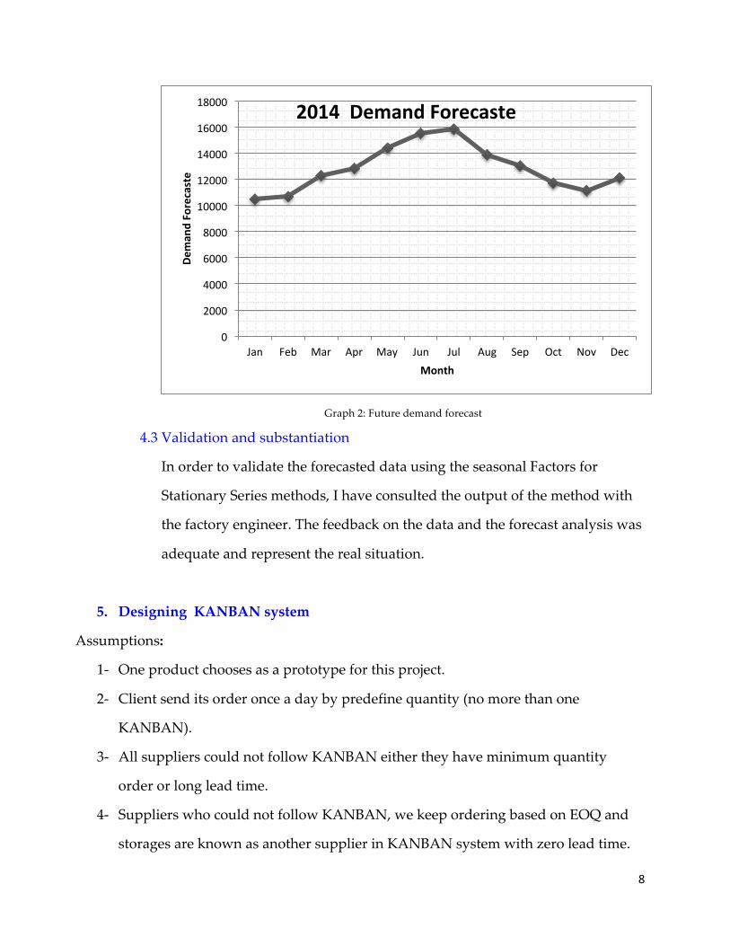
The picture 2 is a snap shot of KANBAN follow between manufacturing and suppliers,
which will design.
Figure 3: Snap shot of a KABAN system
10
5.1 Calculate quantity KANBAN card:
Several methods were defined for calculate quantity KANBAN card
(http://www.resourcesystemsconsulting.com/blog/) (http://www.kanban.com). Based on
available data formula, which was selected to calculate quantity of KANBAN card is:
# KANBAN cards = (Demand*Lead time)*(1+α)/Container Size
The “α” was defined in order to accommodates the error in calculation. This error
includes our error to estimate data and supplier error to respond our order, this factor
accommodate for the theft loses in the system (α is 10% in this project).
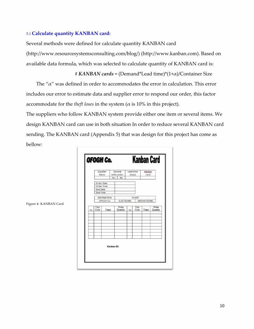
The suppliers who follow KANBAN system provide either one item or several items. We
design KANBAN card can use in both situation In order to reduce several KANBAN card
sending. The KANBAN card (Appendix 5) that was design for this project has come as
bellow:
Figure 4: KANBAN Card
11
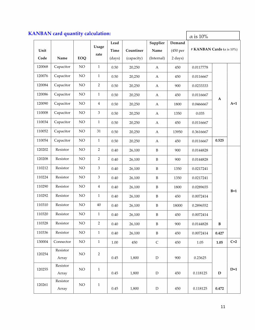
KANBAN card quantity calculation:
Unit
Code Name EOQ
Usage
rate
Lead
Time
(days)
Countiner
(capacity)
Supplier
Name
(Internal)
Demand
(450 per
2 days)
# KANBAN Cards (α is 10%)
120068 Capacitor NO 1 0.50 20,250 A 450 0.0117778
A A=1
120076 Capacitor NO 1 0.50 20,250 A 450 0.0116667
120084 Capacitor NO 2 0.50 20,250 A 900 0.0233333
120086 Capacitor NO 1 0.50 20,250 A 450 0.0116667
120090 Capacitor NO 4 0.50 20,250 A 1800 0.0466667
110008 Capacitor NO 3 0.50 20,250 A 1350 0.035
110034 Capacitor NO 1 0.50 20,250 A 450 0.0116667
110052 Capacitor NO 31 0.50 20,250 A 13950 0.3616667
110054 Capacitor NO 1 0.50 20,250 A 450 0.0116667 0.525
120202 Resistor NO 2 0.40 26,100 B 900 0.0144828
B
B=1
120208 Resistor NO 2 0.40 26,100 B 900 0.0144828
110212 Resistor NO 3 0.40 26,100 B 1350 0.0217241
110224 Resistor NO 3 0.40 26,100 B 1350 0.0217241
110290 Resistor NO 4 0.40 26,100 B 1800 0.0289655
110292 Resistor NO 1 0.40 26,100 B 450 0.0072414
110310 Resistor NO 40 0.40 26,100 B 18000 0.2896552
110320 Resistor NO 1 0.40 26,100 B 450 0.0072414
110328 Resistor NO 2 0.40 26,100 B 900 0.0144828
110336 Resistor NO 1 0.40 26,100 B 450 0.0072414 0.427
130004 Connector NO 1 1.00 450 C 450 1.05 1.05 C=2
120254 Resistor
Array NO 2
0.45 1,800 D 900 0.23625
D D=1 120255
Resistor
Array NO 1
0.45 1,800 D 450 0.118125
120261 Resistor
Array NO 1
0.45 1,800 D 450 0.118125 0.472
α is 10%
12
Unit
Code Nmae EOQ
Usage
rate
Lead
Time
(days)
Countiner
(capacity)
Supplier
Name(Inte
rnal)
Demand(
450 per 2
days)
# KANBAN Cards (α is 10%)
120408 IC OpAmp NO 1 1.10 16,200 E 450 0.0320833
120610 Transistor NO 1 1.10 16,200 E 450 0.0320833
E
E=2
120613 Transistor NO 1 1.10 16,200 E 450 0.0320833
120850 LED NO 1 1.10 16,200 E 450 0.0320833
122000 Crystal NO 1 1.10 16,200 E 450 0.0320833
110426 IC OpAmp NO 1 1.10 16,200 E 450 0.0320833
110430 IC Shift
Register NO 2
1.10 16,200 E 900 0.0641667
110432 IC Shift
Register NO 1
1.10 16,200 E 450 0.0320833
110600 Transistor NO 10 1.10 16,200 E 4500 0.3208333
110604 Transistor NO 2 1.10 16,200 E 900 0.0641667
110902 Diode NO 4 1.10 16,200 E 1800 0.1283333
110904 Diode NO 2 1.10 16,200 E 900 0.0641667
110952 Diode
Supressor NO 9
1.10 16,200 E 4050 0.28875
100000 PCB NO 1 1.50 450 G 450 1.575 1.15
110944 Body NO 1 2.00 450 I 450 2.1 1.5 G=2
110912 Packing box NO 1 0.60 450 K 450 0.63 2 I=2
110418 IC Micro
Controller YES 1
0.6 K=1
110434 IC Sound YES 1
110958 LCD YES 1
200000 Print Screen YES 1/1000
0
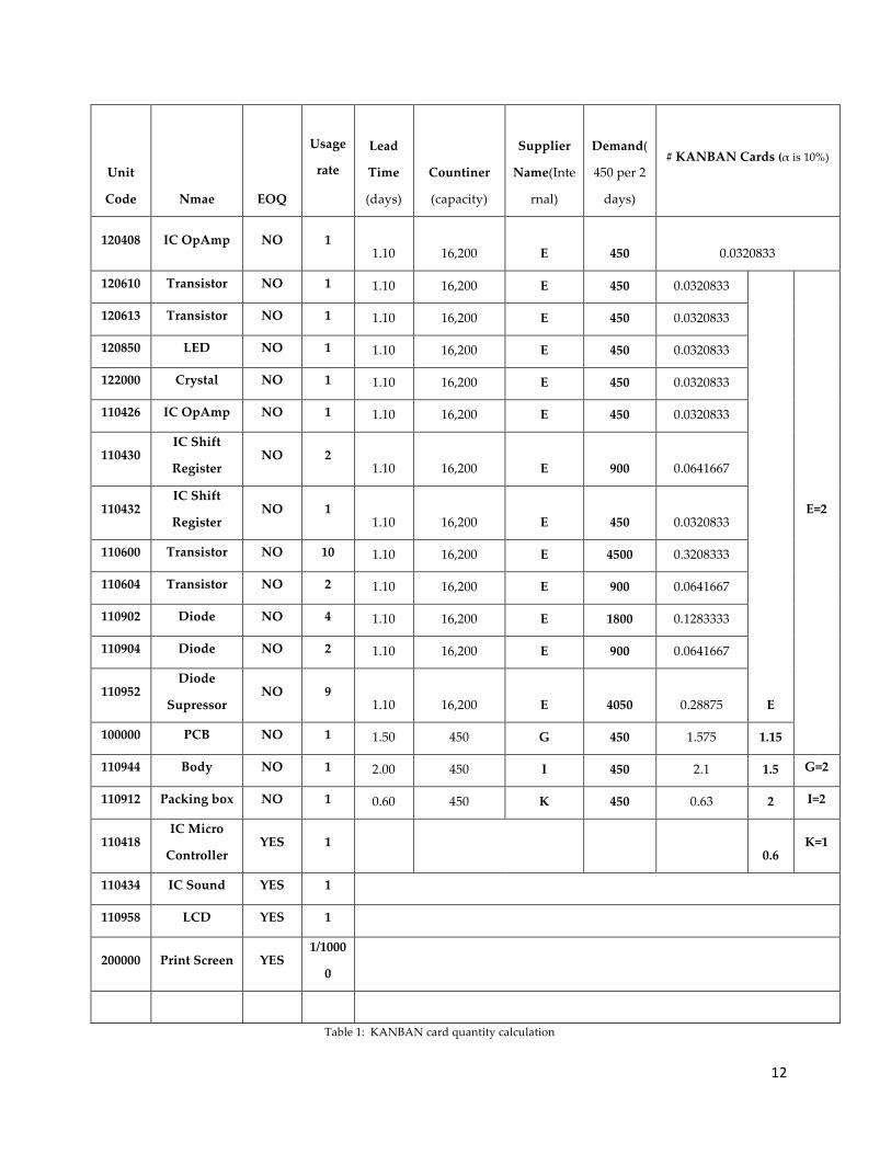
Table 1: KANBAN card quantity calculation
13
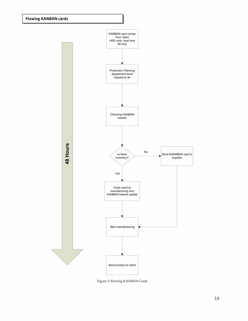
KANBAN card comes from client
(450 units, lead time 48 Hrs)
Production Planning department send
request to all
Is there inventory?
Order send to manufacturing and
KANBAN boards update
Yes
Send KANABAN card to supplier
No
Start manufacturing
Checking KANBAN boards
Send product to client
48 H
ours
Figure 5: Flowing KANBAN Cards
Flowing KANBAN cards
14
6. Cost Analysis:
In order for us to evaluate and present the recommendation, I will be
presenting the current ordering policy cost where Material Requirement
Planning (MRP) is being used (without KANBAN implementation, I will
call it the current situation) and compare it with the cost if KANBAN is
applied to the factor.
6.1 The Cost of the current situation (Without KANBAN implementation).
According to the bill of material and the information provided from the
factory, the list of all components that build the products is as follows;
Capacitors (different Models), Resistors (Different Models), Resistors Array
(Different Models), IC OpAMP (Different Models), Transistor (Different
Models), LED, Crystal, IC Shift Register, Transistor, Diode (Different
Models), Diode Suppressor, PCB, Body, Packing Box, IC Micro-‐‑Controller,
IC Sound, LCD and Print Screen.
All of the above items have different cots, the set up cost is USD 100 per
each and the holding cost is based on an annual interest rate of 40%.
The Economical Order Quantity (EOQ) is defined is as follows;
EOQ = (2KL/h)1/2 , where K is the set up cost, L is the demand and h is the
holding cost based on the intrest rate (I).
The EOQ is determined for each product and is shown in Appendix 3.
The relevant set up and holding cost of this order policy is determined
according to the cost function of the EOQ (KL/EOQ + EOQ*h/2) where k set
up cost, L Demand & Holding Cost. The resulted total monthly cost is equal
to USD 1,287,882.
6.2 The cost if KANBAN to be applied to the factory.
6.2.1 Cost resulted from the suppliers who didn’t follow the KANBAN.
15
The supplier who didn’t follow the KANBAN in this project are
those supporting the factory with the following items
i. IC Micro-‐‑Controller
ii. IC Sound
iii. LCD
iv. Print Screen
The factory will continue ordering the above mentioned items directly
from the suppliers, the Economic Order Quantity will be the model
followed to determine the order quantity.
i. For the IC Micro-‐‑Controller, each item -‐‑ according to the
information provided from the factory-‐‑ cost USD 6.5 and
according to the forecasted demand for year 2011, the annual
demand is 154000 units. From the experience and the information
provided from the factory the set up cost is USD 652, the cost of
this item is high due to that the supplier are all from outside
Saudi Arabia. The annual interest rate was assumed 40%
annually.
Knowing that EOQ = (2KL/h)1/2 , where K is the Set Up cost, L is
the demand and h is the holding cost based on the interest rate
(I), I Applied the EOQ formula and results that the economic
ordering quantity of the IC Micro-‐‑Controller is 8788 Units.
The resulted set up and holding from this ordering policy for
the IC Micro-‐‑Controller is USD 22,850. That is resulted from
applying the cost formula of the holding and set up cost.
ii. For the IC Sound, the cost of each item is USD 3.5. The set up
cost is USD 652, while the forecasted annual demand is 154000
units. Knowing that EOQ = (2KL/h)1/2 , where K is the Set Up
16
cost, L is the demand and h is the holding cost based on the
intrest rate (I), we apply the Economical Order Quantity (EOQ)
formula results in 11,977 units.
The relevant set up and holding cost of this item’s ordering
policy is USD 16,767.
iii. For the LCD, the cost of each item is USD 10. The annual
forecasted demand is 154000 unites. The Economical Order
Quantity (EOQ= [2KL/h] 1/2 ) for this item is 7085 units. The
related set up and holding cost is USD 28,342.
The total cost using the EOQ for the supplier who didn’t follow
the KANBAN system is USD 68,360.
The supported tables for the calculation of the EOQ are supported in the
appendices under Appendix 4.
6.2.2 The KANBAN Cost
If company use the KANBAN, KANBAN will apply to the
following [Capacitors (different Models), Resistors (Different
Models), Resistors Array (Different Models), IC OpAMP (Different
Models), Transistor (Different Models), LED, Crystal, IC Shift
Register, Transistor, Diode (Different Models), Diode Suppressor,
PCB, Body and Packing Box] each KANBAN is assumed to have
450 units, and the cost of each KANBAN card is estimated to be
USD 100.
Knowing from the forecast of 2011 that the annual demand is
154000 units, we know that the number of the KANBANS that will
be issued are 342 (154000/450) KANBANs. The Cost of all
KANBANS is USD 34,222.
17
As I know from the factory that there is a 13 group of KANBANS,
thus; the relevant cost of applying the KANBAN is USD 444,889.
6.3 Storage Space Cost
In order to calculate the storage space cost, we have to calculate the
storage space first. Gathering some information are important to
come up with final space like the standard of pallet dimension ,the
final product dimension, how many pallets can we put above each
other and how many rows each pallet has.
Here some data that we collected and assumptions that we assumed
in order to get the final storage cost we need.
Data collection:
1-‐‑ Final product dimension is 30cmX20cmX10cm
2-‐‑ U.S Pallet standard Dimension is 1.2mX1mX0.15m
3-‐‑
Assumptions:
1-‐‑ Only allow to put three pallets above each other.
2-‐‑ Each pallet has four rows (shelves).
Therefore, each pallet can takes 80 products (5X4X4).
In addition to that, we have to know the highest monthly
production to build our storage based on that capacity, adding to
that plus 10% as a percentage of error. The highest monthly
production is in July which is equal 15850. Therefore we have to
find space for 17435 products (including 10% of error).
As we calculate above, each pallet can takes 80 products, so we need
218 pallets (17435/80) and only three pallets can we put above each
other, therefore, the aggregate pallet per unit is73 pallets on the floor
18
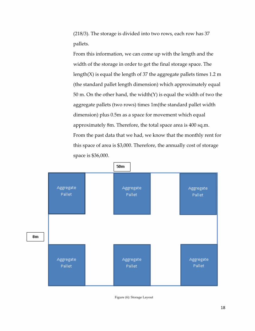
(218/3). The storage is divided into two rows, each row has 37
pallets.
From this information, we can come up with the length and the
width of the storage in order to get the final storage space. The
length(X) is equal the length of 37 the aggregate pallets times 1.2 m
(the standard pallet length dimension) which approximately equal
50 m. On the other hand, the width(Y) is equal the width of two the
aggregate pallets (two rows) times 1m(the standard pallet width
dimension) plus 0.5m as a space for movement which equal
approximately 8m. Therefore, the total space area is 400 sq.m.
From the past data that we had, we know that the monthly rent for
this space of area is $3,000. Therefore, the annually cost of storage
space is $36,000.
Figure (6): Storage Layout
19
Conclusion:
1-‐‑ Based on cost analysis by using KANBAN system we have 50% decreases
in average costs.
2-‐‑ Based on calculation in storage space by using KANBAN system we can
eliminate storage for final goods and we cut monthly rent.
3-‐‑ The method used for forecasting the demand (Seasonal Factors) was
representing the trend that the product is experiencing. We recommend
that this method to be used for forecasting the other automobile related
materials in this factory.
Recommendation:
Based on conclusion it looks scenario one is feasible but it needs follow a roadmap
and specific plan.
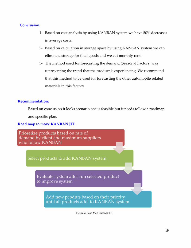
Road map to move KANBAN JIT:
Figure 7: Road Map towards JIT.
Prioretize products based on rate of demand by client and maximum suppliers who follow KANBAN
Select products to add KANBAN system
Evaluate system after run selected product to improve system
Add new peoduts based on their priority until all products add to KANBAN system
20
References
Nahmias. 2008. Production and operation analysis. (6 edition ed.). McGraw-Hill/Irwin. Ragsdale, Cliff T. 2003. Spreadsheet modeling & decision analysis. Practical introduction to management science. (4 ed.). South-Western College Pub. Ahad Ali, Mohammad Khadem, and Neriliz Santini 2010. Kanban Supplier System as a
Standardization Method and WIP Reduction. International Conference on Industrial Engineering and Operations Management.
Resource Systems Group. 2011. Kanban Calculation. From <http://www.resourcesystemsconsulting.com>.