Embed Size (px)
Citation preview
MPRAMunich Personal RePEc Archive
Interaction of carbon and electricityprices under imperfect competition
Liliya Chernyavs’ka and Francesco Gull̀ı
IEFE (Centre For Research on Energy and EnvironmentalEconomics and Policy) - Bocconi University
May 2007
Online at http://mpra.ub.uni-muenchen.de/5866/MPRA Paper No. 5866, posted 22. November 2007 06:06 UTC

Università Commerciale Luigi Bocconi IEFE Istituto di Economia e Politica dell’Energia e dell’Ambiente
WORKING PAPER SERIES
www.iefe.unibocconi.it
Interaction of carbon and electricity prices under imperfect competition
Liliya Chernyavs’ka, Francesco Gullì
Working Paper N.2
May 2007

Interaction of carbon and electricity prices under imperfect competition
Liliya Chernyavs’ka, DIEM, University of Genoa* Francesco Gullì, IEFE, Bocconi University**
May 2007
Abstract
In line with economic theory, carbon ETS determines a rise in marginal cost equal to the carbon opportunity cost regardless of whether carbon allowances are allocated free of charge or not. Hence, common sense would suggest that .rms in imperfectly competitive markets will pass-through into electricity prices only a part of the increase in cost. Instead, by using the load duration curve approach and the dominant .rm with competitive fringe model, the analysis proposed in this paper shows that the result is ambiguous. The increase in price can be either lower or higher than the marginal CO2 cost depending on several structural factors: the degree of market concentration, the available capacity (whether there is excess capacity or not) and the power plant mix in the market; the allowance price and the power demand level (peak vs. off-peak hours). The empirical analysis of the Italian context (an emblematic case of imperfectly competitive market), which can be split in four sub-markets with different structural features, confirms the model predictions. Market power, therefore, can determine a significant deviation from the "full pass-through" rule but we can not know which is the sign of this deviation, a priori, i.e. without before carefully accounting for the structural features of the power market. Keywords: Emission trading, power pricing, imperfect competition JEL classification: L13, Q21, Q41 *Corresponding author: DIEM – Università di Genova, Via Vivaldi, 5, 16126 Genova, Italy, [email protected] **Corresponding author: IEFE – Università Bocconi, Viale Filippetti, 9, 20122 Milano, Italy. Tel.: +39 02 58363820-1; fax +39 02 58363890; [email protected]
Interaction of carbon and electricity prices under imperfect competition
Liliya Chernyavs�ka� Francesco Gull�
�DIEM-University of Genoa, via Vivaldi 5, 16126 Genoa (Italy)
��Iefe-Bocconi University, Viale Filippetti 9, 20122 Milan (Italy): e-mail:
1. Introduction
Power generation is the largest industry sector covered by the European Union CO2
emissions trading scheme (EU ETS)1 . Therefore, on the one hand, the performance of
the ETS largely depends on its e¢ cacy in inducing power industry to signi�cantly reduce
CO2 emissions. On the other hand, the ETS might have a sensible impact on power prices
and, consequently, on social welfare.
This study focuses on this latter issue, attempting to understand how a CO2 price could
impact on power pricing when electricity markets are imperfectly competitive2 . Studies
aimed at exploring this issue do exist but they provide a very controversial framework.
On the theoretical side, Sijm et al. (2005) and Wals and Rijkers (2003) �nd that
the electricity price in a competitive scenario increases more than under market power,
on both percentage and absolute basis3 . They attribute this result to the assumption
of linear demand function they adopt. Surprisingly, however, Lise (2005) achieves the
opposite result (electricity price increases more under market power) even though the
author use the same model. Reinaud (2003), relying on price competition, and Newbery
(2005), by assuming constant price elasticity, states that electricity prices are likely to
increase more under market power.1The EU ETS started in 2005. In the period 2005-2007, each European country allocates allowances
to eligible �rms. At least 95% of the total amount of allowances are allocated free of charge and �rms can
use or trade them. At the end of each calendar year each eligible �rm must deliver a number of allowances
corresponding to his total emissions in that year. At the beginning of 2008 a new ETS starts and the old
allowances become worthless.2Many authors deal with the link between market structure and environmental issues. For a survey,
see also Requate (2005).3The aurhors use a game theoretical simulation model based on the theory of Cournot competition and
Conjecture Supply Funcions, the COMPETES model. For details on this model, see Day et al. (2002),
Hobbs and Rijkers (2004a; 2004b).
1
Interaction of carbon and electricity prices under imperfect competition 2
On the empirical side, there are not speci�c studies aimed at measuring the impact
of market power. Most analyses try to check whether CO2 costs are fully passed through
into electricity prices or not and generically attribute the "deviation" from this "rule" to
various factors among which the exercise of market power in the output markets.
In this paper, we speci�cally attempt to assess the impact of market power by us-
ing a simple theoretical model and subsequently checking its robustness by means of an
empirical analysis.
Concerning the theoretical issues, we have to be aware that results signi�cantly de-
pends on the choice of the competition model4 .
In the present work we will follow the suggestion of authors who argue in favour of
adopting the "auction" approach (von der Fehr and Harbord, 1993, 1998). In fact, several
electricity spot markets have characteristics which make standard models not well-suited
to their analysis. In particular in these markets pricing mechanism is a uniform, �rst price
auction.
In addition, to simulate market power in electricity markets we use a dominant �rm
facing a competitive fringe model rather than the usual dupolistic-oligopolistic frame-
work. This choice is due to several reasons, either methodological or practical. On the
methodological side, the attraction of this characterization is that it avoids the implau-
sible extreme of perfect competition and pure monopoly, at the same time escaping the
di¢ culties of characterizing an oligopolistic equilibrium5 . On the practical side, it is well
suited to simulate the structural features of the Italian market which is the empirical case
analysed in this paper6 .
4 In particular, price elasticity choice is very important in simulating the impact of the ETS and can
undermine the e¤ectiveness of a model. For example, the existence of Nash equilibria within the Cournot
model requires substantial negative price elasticity. This is the case, for example, of the COMPETES
model cited above. Whereas completely inelastic demand seems to be more appropriate for the power
industry, at least in the short-run. Moreover, Bolle (1992) proves that in this latter case no equilibrium
exists in the supply-function model.5 In particular, this model allows us to overcome the problem of possible inexistent equilibria in pure
strategy. In their article on spot market competition in the UK electricity industry, using a typical
duopolistic framework, von der Fehr and Harbord (1993) demonstrate that under variable-demands period
(i.e. when the range of possible demands exceeds the capacity of the largest generator) there does not
exist an equilibruim in pure strategy. Instead, there exist a unique mixed-strategy Nash equilibrium.6 Indeed, the dominant �rm-competitive fringe model is useful to represent the reality of several power
markets. We especially refer to those markets emerging from restructuring processes where the incumbent
Interaction of carbon and electricity prices under imperfect competition 3
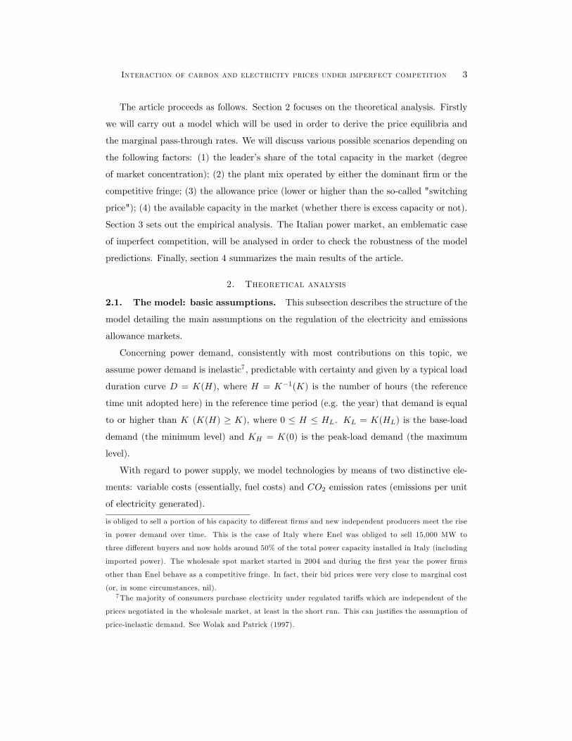
The article proceeds as follows. Section 2 focuses on the theoretical analysis. Firstly
we will carry out a model which will be used in order to derive the price equilibria and
the marginal pass-through rates. We will discuss various possible scenarios depending on
the following factors: (1) the leader�s share of the total capacity in the market (degree
of market concentration); (2) the plant mix operated by either the dominant �rm or the
competitive fringe; (3) the allowance price (lower or higher than the so-called "switching
price"); (4) the available capacity in the market (whether there is excess capacity or not).
Section 3 sets out the empirical analysis. The Italian power market, an emblematic case
of imperfect competition, will be analysed in order to check the robustness of the model
predictions. Finally, section 4 summarizes the main results of the article.
2. Theoretical analysis
2.1. The model: basic assumptions. This subsection describes the structure of the
model detailing the main assumptions on the regulation of the electricity and emissions
allowance markets.
Concerning power demand, consistently with most contributions on this topic, we
assume power demand is inelastic7 , predictable with certainty and given by a typical load
duration curve D = K(H), where H = K�1(K) is the number of hours (the reference
time unit adopted here) in the reference time period (e.g. the year) that demand is equal
to or higher than K (K(H) � K), where 0 � H � HL. KL = K(HL) is the base-load
demand (the minimum level) and KH = K(0) is the peak-load demand (the maximum
level).
With regard to power supply, we model technologies by means of two distinctive ele-
ments: variable costs (essentially, fuel costs) and CO2 emission rates (emissions per unit
of electricity generated).
is obliged to sell a portion of his capacity to di¤erent �rms and new independent producers meet the rise
in power demand over time. This is the case of Italy where Enel was obliged to sell 15,000 MW to
three di¤erent buyers and now holds around 50% of the total power capacity installed in Italy (including
imported power). The wholesale spot market started in 2004 and during the �rst year the power �rms
other than Enel behave as a competitive fringe. In fact, their bid prices were very close to marginal cost
(or, in some circumstances, nil).7The majority of consumers purchase electricity under regulated tari¤s which are independent of the
prices negotiated in the wholesale market, at least in the short run. This can justi�es the assumption of
price-inelastic demand. See Wolak and Patrick (1997).
Interaction of carbon and electricity prices under imperfect competition 4
In particular, CO2 emission rate is e � 0 and variable cost of production is v � 0 for
production levels less than capacity, while production above capacity is impossible (i.e.
in�nitely costly).
Since we simulate a uniform, �rst price auction, it su¢ ces focusing on technologies
which have a positive probability of becoming the marginal operating unit. This allows
us to neglect, without loss of generality, those technologies suited to meet the base-load
demand (i.e. nuclear and large hydropower plants, renewable technologies, cogeneration
plants and so on) or which are inelastically supplied.
Given these premises, we restrict the analysis to two groups of plants, a and b, and
assume that each group includes a very large number n of homogeneous generating units8
such that
Kj =P
i=1;2::n kij = nkj , j = a; b and v
ij = vj ; e
ij = ej ;8i; j
where vij = vj > 0 and kij = kj > 0 are the variable cost and the capacity of the i-th
unit belonging to the group j, respectively. Thus Ka and Kb are the installed capacity of
groups a and b, respectively.
Furthermore, we assume va < vb and Ka+Kb = KH , i.e. the units of kind a and b are
su¢ cient to meet the peak demand, and consider two scenarios: Scenario 1 in which there
is trade-o¤ between variable costs and emission rates (hereafter "trade-o¤ in the plant
mix"), i.e. the technology with lower variable cost is the worse polluter (va < vb and
ea > eb, a typical relevant example is given by coal plants (a) versus CCGT -combined
cycle gas turbine- technologies (b)); Scenario 2 in which there is not such a trade-o¤, i.e.
the technology with lower variable cost is also the cleaner technology (va < vb but ea < eb,
a typical relevant example is given by CCGT plants (a) versus steam cycle plants (b)).
These two scenarios are well suited to represent the Italian market which is the context
used for the empirical analysis.
Emission abatement is supposed to be impossible or, equivalently, abatement cost
in�nitely costly. This hypothesis is consistent with the time horizon of the analysis (short
term analysis of the ETS impact).
Concerning the wholesale market, we assume a typical day ahead market. Before
the actual opening of the market (e.g. the day ahead) the generators simultaneously
8Assuming that each group includes the same number n of units implies that kj depends on Kj : This
is an arbitrary assumption which does not undermine, however, the signi�cance of the analysis.
Interaction of carbon and electricity prices under imperfect competition 5
submit bid prices for each of their units on hourly basis. We neglect the existence of
technical constraints such as start-up costs. The auctioneer (generally the so-called market
operator) collects and ranks the bids by applying the merit order rule. The bids are
ordered by increasing bid prices and form the basis upon which a market supply curve is
carried out.
If called upon to supply, generators are paid according to the market-clearing spot
price (the system marginal price, equal to the highest bid price accepted). All players
are assumed to be risk neutral and to act in order to maximize their expected payo¤
(pro�t). Production costs, emission rates as well as plants�installed capacity are common
knowledge.
Given the regulatory framework described above, it is straightforward that price equi-
libria will depend on the power demand level. Since this latter continuously varies over
time, an useful way of representing the price schedule is carrying out the so-called price
duration curve p(H) where H is the number of hours in the year that the power price is
equal to or higher than p.
With regard to the allowance market, we suppose this market is very large (consistently
with the extent of the European ETS) and that �rms are price takers. Therefore, the
allowance price, ptp, is given exogenously. Carbon emissions allowances are allocated free
of charge and on the basis of the amounts emitted in a base period, generally a year in the
past (typical grandfathering) or the present year or on the basis of the expected emissions
in the future9 .
Finally, we assume that �rm�s o¤er prices are constrained to be below some threshold
level, bp; which can be interpreted in several ways.It may be a (regulated) maximum price, p, as o¢ cially introduced by the regulator or
we can suppose that it is not introduced o¢ cially but simply perceived by the generators,
i.e. �rms believe that the regulator will introduce price regulation if the price rises above
the threshold. This latter interpretation is well-suited to the topic analysed here. In fact,
�rms might decide to bring bid prices down not only to avoid regulation in the wholesale
electricity market but also to avoid a change in the allowance allocation method, e.g.
from freely allocation to auctioning10 . For these reasons we think that it is acceptable
9For a comparative analysis of the di¤erent allocation methods, see Harrison and Radov (2002) and
Burtraw et al. (2001).10For instance, in Germany, where there is a controversial debate on this topic, Eon, one of the leading

Interaction of carbon and electricity prices under imperfect competition 6
assuming the price cap is insensitive to the CO2 price.
Alternatively, we can suppose that there is so much generation that price never is
above the marginal cost of a peaker. In order to simulate this situation, we introduce
a third technology, c, such that vc > max [va; vb] and whose capacity is great enough,
Kc = Kc; that the dominant �rm does not try to let it all run and drive the price up to
the price cap. Instead, Kc = 0; is useful to simulate the situation in which there is not
excess capacity in the market and prices can reach the price cap, p. Finally, we assume
that ea > ec > eb in the Scenario 1 and ec > eb > ea in the Scenario 2. These choices are
crucial for our analysis but not arbitrary. Technoogy c, in fact, can be interpreted as a
typical peaking technology (in the Italian market, old oil-�red plants or gas turbine plants)
whose electrical e¢ ciency is generally much lower than that of the CCGT. Furthermore,
this technology is generally more polluting than CCGT (or gas-�red steam cycle plants)
but cleaner than coal plants.
In brief, we will consider two scenarios (Scenario 1 and Scenario 2, with and without
"trade-o¤ in the plant mix", respectively) and, for each of them, two cases of available
capacity in the market, excess capacity (Kc = Kc) and scarcity of generation capacity
(Kc = 0):
2.2. Price duration curves. In order to derive price equilibria in the form of price
duration curves, we have to start from how the ETS impacts on marginal production
costs. Given that an emission allowance represents an opportunity cost, the marginal
cost of production is expected to include the full carbon opportunity cost, regardless of
whether allowances are allocated free of charge or not. Formally,
MCij = vij + p
tpeij (1)
where MCij is the marginal cost of the i-th unit belonging to the group j of plants and
ptpeij is the corresponding carbon opportunity cost.
Given equation (1) and for the purpose of this analysis, the generating units belonging
to the group j of plants are the most (least) e¢ cient units if their marginal cost (including
the carbon opportunity cost) is lower (higher) than that of the units belonging to the other
group i.
power �rms, argues that "there is no scope to remove windfall pro�ts from the EU-ETS, only redistribute
them, so e¤orts should be focused on bringing the electricity price down".
Interaction of carbon and electricity prices under imperfect competition 7
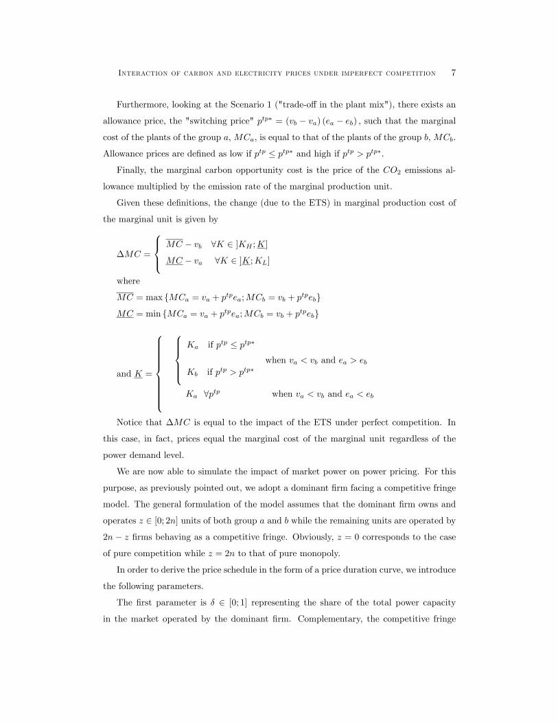
Furthermore, looking at the Scenario 1 ("trade-o¤ in the plant mix"), there exists an
allowance price, the "switching price" ptp� = (vb � va) (ea � eb) ; such that the marginal
cost of the plants of the group a, MCa; is equal to that of the plants of the group b, MCb:
Allowance prices are de�ned as low if ptp � ptp� and high if ptp > ptp�:
Finally, the marginal carbon opportunity cost is the price of the CO2 emissions al-
lowance multiplied by the emission rate of the marginal production unit.
Given these de�nitions, the change (due to the ETS) in marginal production cost of
the marginal unit is given by
�MC =
8><>:MC � vb 8K 2 ]KH ;K]
MC � va 8K 2 ]K;KL]
where
MC = max fMCa = va + ptpea;MCb = vb + ptpebg
MC = min fMCa = va + ptpea;MCb = vb + ptpebg
and K =
8>>>>>>>><>>>>>>>>:
8>>><>>>:Ka if ptp � ptp�
Kb if ptp > ptp�when va < vb and ea > eb
Ka 8ptp when va < vb and ea < eb
Notice that �MC is equal to the impact of the ETS under perfect competition. In
this case, in fact, prices equal the marginal cost of the marginal unit regardless of the
power demand level.
We are now able to simulate the impact of market power on power pricing. For this
purpose, as previously pointed out, we adopt a dominant �rm facing a competitive fringe
model. The general formulation of the model assumes that the dominant �rm owns and
operates z 2 [0; 2n] units of both group a and b while the remaining units are operated by
2n � z �rms behaving as a competitive fringe. Obviously, z = 0 corresponds to the case
of pure competition while z = 2n to that of pure monopoly.
In order to derive the price schedule in the form of a price duration curve, we introduce
the following parameters.
The �rst parameter is � 2 [0; 1] representing the share of the total power capacity
in the market operated by the dominant �rm. Complementary, the competitive fringe
Interaction of carbon and electricity prices under imperfect competition 8
)(HK
K
HK
LHH fHH
dH KKK −=
fd KKK +=
LK
H
fK
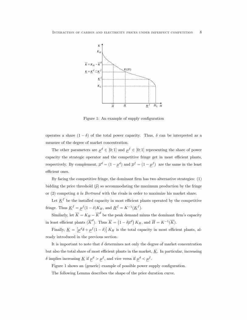
Figure 1: An example of supply con�guration
operates a share (1� �) of the total power capacity. Thus, � can be interpreted as a
measure of the degree of market concentration.
The other parameters are �d 2 [0; 1] and �f 2 [0; 1] representing the share of power
capacity the strategic operator and the competitive fringe get in most e¢ cient plants,
respectively. By complement, �d = (1� �d) and �f = (1� �f ) are the same in the least
e¢ cient ones.
By facing the competitive fringe, the dominant �rm has two alternative strategies: (1)
bidding the price threshold (bp) so accommodating the maximum production by the fringe
or (2) competing à la Bertrand with the rivals in order to maximize his market share.
Let Kf be the installed capacity in most e¢ cient plants operated by the competitive
fringe. Thus Kf = �f (1� �)KH , and Hf = K�1(Kf ).
Similarly, let K = KH �Kdbe the peak demand minus the dominant �rm�s capacity
in least e¢ cient plants (Kd). Thus K =
�1� ��d
�KH , and H = K�1(K).
Finally, K =��d� + �f (1� �)
�KH is the total capacity in most e¢ cient plants, al-
ready introduced in the previous section.
It is important to note that � determines not only the degree of market concentration
but also the total share of most e¢ cient plants in the market, K. In particular, increasing
� implies increasing K if �d > �f ; and vice versa if �d < �f .
Figure 1 shows an (generic) example of possible power supply con�guration.
The following Lemma describes the shape of the price duration curve.
Interaction of carbon and electricity prices under imperfect competition 9
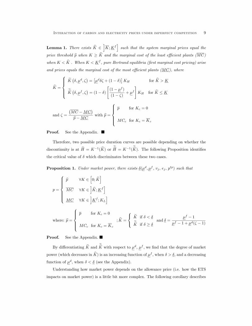
Lemma 1. There exists bK 2iK;Kf
isuch that the system marginal prices equal the
price threshold bp when K � bK and the marginal cost of the least e¢ cient plants (MC)
when K < bK . When K < Kf , pure Bertrand equilibria (�rst marginal cost pricing) arise
and prices equals the marginal cost of the most e¢ cient plants (MC), where
bK =
8>>><>>>:eK ��; �d; �� = ��d�� + (1� �)�KH for bK > K
eeK ��; �f ; �� = (1� �)" (1� �f )(1� �) + �
f
#KH for bK � K
and � =
�MC �MC
�bp�MC with bp =
8>>><>>>:p for Kc = 0
MCc for Kc = Kc
Proof. See the Appendix.
Therefore, two possible price duration curves are possible depending on whether the
discontinuity is at eH = K�1( eK) or eeH = K�1(eeK). The following Proposition identi�es
the critical value of � which discriminates between these two cases.
Proposition 1. Under market power, there exists �(�d; �f ; vj ; ej ; ptp) such that
p =
8>>>>><>>>>>:bp 8K 2
h0; bKi
MC 8K 2i bK;Kf
iMC 8K 2
iKf ;KL
i
where: bp =8>>><>>>:p for Kc = 0
MCc for Kc = Kc
; bK =
8<: eK if � < �eeK if � � �and � =
�f � 1�f � 1 + �d(� � 1)
Proof. See the Appendix.
By di¤erentiating eK and eeK with respect to �d, �f , we �nd that the degree of market
power (which decreases in bK) is an increasing function of �f , when � > �, and a decreasingfunction of �d, when � < � (see the Appendix):
Understanding how market power depends on the allowance price (i.e. how the ETS
impacts on market power) is a little bit more complex. The following corollary describes
Interaction of carbon and electricity prices under imperfect competition 10
this kind of correlation under low allowance prices11 (the most relevant case for the em-
pirical analysis of this paper).
Corollary 1. Under low allowance prices, the ETS determines an increase in market
power ( bK decreases in ptp) if (e � ea)=(v � va) > (eb � ea)=(vb� va), where: e = ec and
v = vc, under excess capacity; e = 0 and v = p, without excess capacity.
Proof. For the formal proof, see the Appendix. Intuitively, the ETS can increase
market power when the change in the cost structure between the technologies makes
more pro�table bidding the price threshold rather than the marginal cost of the least
e¢ cient plants, i.e. when (e � ea)=(v � va) > (eb � ea)=(vb� va). This condition always
(never) is satis�ed if "trade-o¤ in the plant mix" combines with excess capacity (without
both "trade-o¤ in the plant mix" and excess capacity). Otherwise, it is satis�ed only
under certain values of vj and ej .
2.3. Marginal pass-through rate. Since we intend to consider the overall change
in marginal prices due the ETS, an useful way of proceeding is evaluating the marginal
pass-through rate de�ned as follows.
De�nition 1. The marginal pass-through rate (MPTR) is the change in power prices,
4p; divided by the change in marginal production costs of the marginal unit, �MC; due
to the ETS.
Notice that the MPTR is always equal to 1 under perfect competition. In this case, in
fact, prices equal the marginal cost of the marginal unit regardless of the power demand
level.
Table 1: Parameter expressions before and after the ETS
11When allowance prices are high the framework is even more complex. Since understanding how the
ETS impacts on market power under all conditions is beyond the scope of this paper, we neglect the
formal analysis of what can occur under high allowance prices.
Interaction of carbon and electricity prices under imperfect competition 11
Before ETS Scenario 1 Scenario 2
ptp = 0 ptp � ptp� ptp > ptp� 8ptp
MCc vc MCc MCc MCc
MC vb MCb MCa MCb
MC va MCa MCb MCa
�d �da �da �db �da
�f �fa �fa �fb �fa
In order to carry out the MPTR curve (i.e. how the MPTR is distributed over time), we
have to depict the price and marginal cost (of the marginal unit) duration curves before
and after the ETS distinguishing between low (0 < ptp � ptp�) and high (ptp > ptp�)
allowance prices (only for the Scenario 1). Table 1 shows the di¤erent expressions of
MCc; MC, MC, �d, �f corresponding to the situations after and before the ETS. We
will use the superscript star (*) in order to address the critical threshold of K, H, and �
when ptp 6= 0 (i.e. the situation after the ETS).
In what follows, we will present some relevant examples of marginal pass-through
rate curves corresponding to di¤erent scenarios in terms of available capacity, market
concentration and plant mix. For the sake of simplicity, we will illustrate only the outcome
under low allowance prices while that under high allowance prices is reported in the
Appendix.
Scenario 1 ("trade-o¤ in the plant mix"): low allowance prices. In this case,bK always decreases in ptp under excess capacity whereas may either decrease or increase
under scarcity of generation capacity (see proof of Corollary 1): We refer to increasing
market power because this is the most likely situation given the plausible plant mix in
the market: coal plants (a), CCGT (b) and oil-�red plants (c): In fact, by using the
emission rates and variable costs of these technologies (tab. 4 in the Appendix), we get
(e� ea)=(v� va) > (eb � ea)=(vb� va); regardless of the available capacity in the market.
Thus, three relevant con�gurations (corresponding to three possible values of market
concentration) have to be analysed (see Lemma 1 and Proposition 1): eK > eK� > K
(� < �� < �); eK > K >eeK�(�� < � < �); K >
eeK >eeK�(�� < � < �).
Figures 2 and 3 illustrate the MPTR curves obtained by deviding the change in prices
Interaction of carbon and electricity prices under imperfect competition 12
p
H LH HH~ *~H
δδδ << *
H HH
fH H
δδδ <<*p
H LHH~ *~~H
δδδ <<*
fH
p
HH LHH~~ *~~H
fH
≈
p
≈ ≈
p p
≈
≈ ≈ ≈ ≈
≈ ≈≈
1 11
MPTR MPTR MPTR
≈ ≈ ≈
Market Power (Before ETS)
Marginal cost of the marginal unit(Before ETS)
Market Power (After ETS)
Marginal cost of the marginal unit(After ETS)
bMC
aMCbv
av
bMC
aMCbv
av
bMC
aMCbv
av
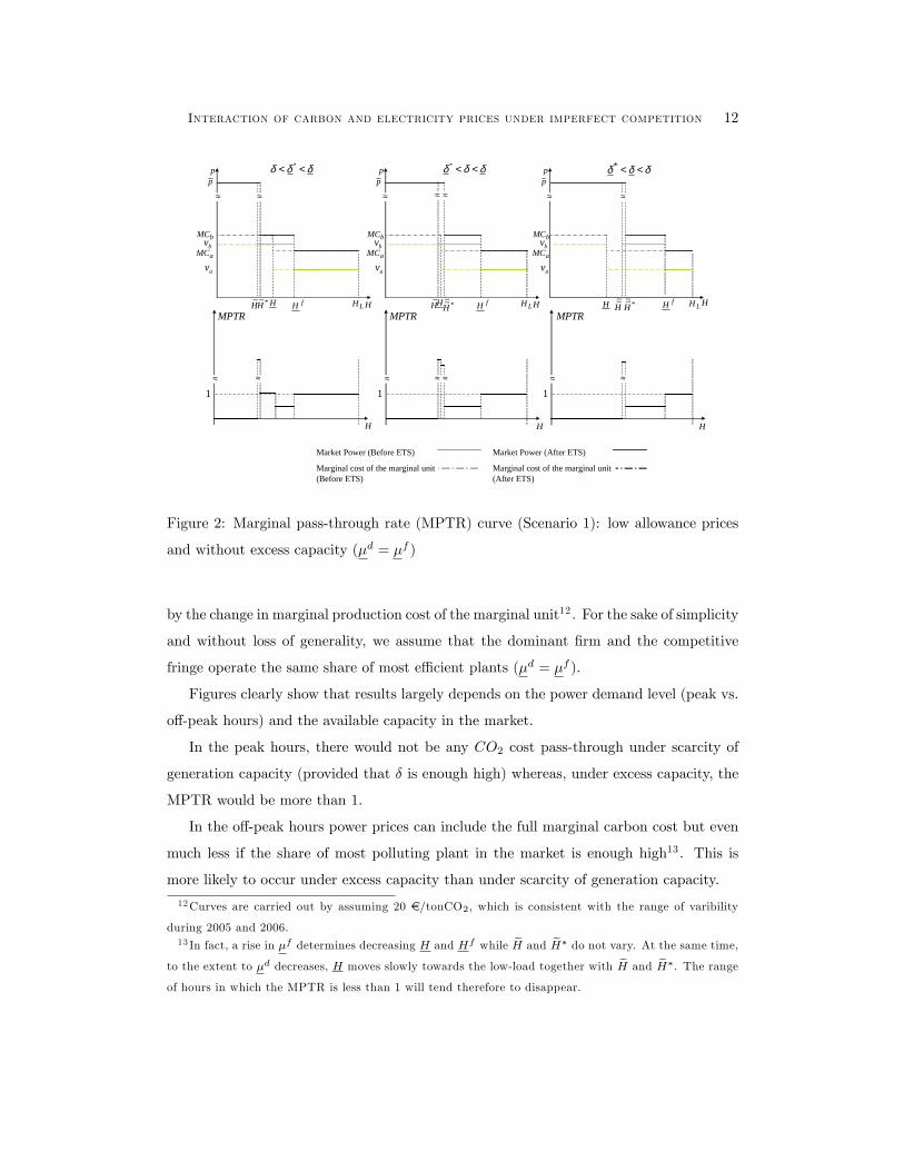
Figure 2: Marginal pass-through rate (MPTR) curve (Scenario 1): low allowance prices
and without excess capacity (�d = �f )
by the change in marginal production cost of the marginal unit12 . For the sake of simplicity
and without loss of generality, we assume that the dominant �rm and the competitive
fringe operate the same share of most e¢ cient plants (�d = �f ).
Figures clearly show that results largely depends on the power demand level (peak vs.
o¤-peak hours) and the available capacity in the market.
In the peak hours, there would not be any CO2 cost pass-through under scarcity of
generation capacity (provided that � is enough high) whereas, under excess capacity, the
MPTR would be more than 1.
In the o¤-peak hours power prices can include the full marginal carbon cost but even
much less if the share of most polluting plant in the market is enough high13 . This is
more likely to occur under excess capacity than under scarcity of generation capacity.
12Curves are carried out by assuming 20 e/tonCO2, which is consistent with the range of varibility
during 2005 and 2006.13 In fact, a rise in �f determines decreasing H and Hf while eH and eH� do not vary. At the same time,
to the extent to �d decreases, H moves slowly towards the low-load together with eH and eH�. The range
of hours in which the MPTR is less than 1 will tend therefore to disappear.
Interaction of carbon and electricity prices under imperfect competition 13
p
H LH HH~ *~H
H HH
fH H
p
H LHH~ *~~HfH
p
HH LHH~~ *~~H
fH
bMC
aMCbv
av
cvcMC
δδδ << * δδδ <<*δδδ <<*
1 1 1
MPTR MPTR MPTR
Market Power (Before ETS)
Marginal cost of the marginal unit(Before ETS)
Market Power (After ETS)
Marginal cost of the marginal unit(After ETS)
bMC
aMCbv
av
cvcMC
bMC
aMCbv
av
cvcMC
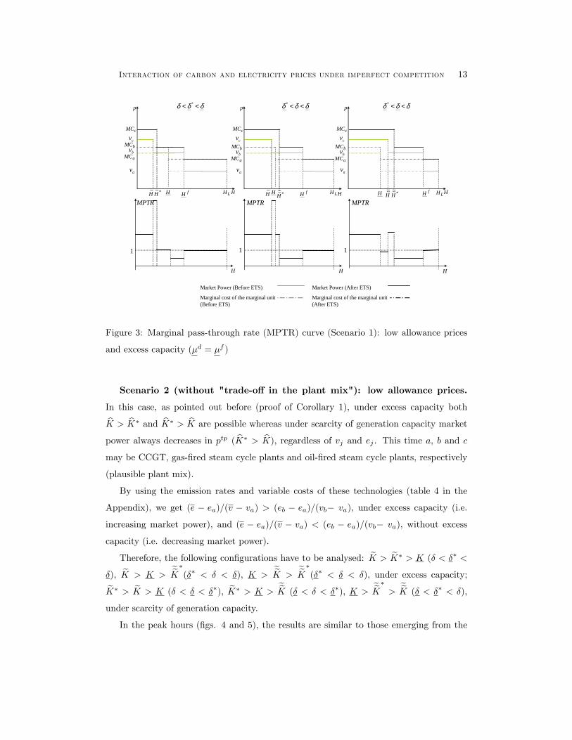
Figure 3: Marginal pass-through rate (MPTR) curve (Scenario 1): low allowance prices
and excess capacity (�d = �f )
Scenario 2 (without "trade-o¤ in the plant mix"): low allowance prices.
In this case, as pointed out before (proof of Corollary 1), under excess capacity bothbK > bK� and bK� > bK are possible whereas under scarcity of generation capacity market
power always decreases in ptp ( bK� > bK); regardless of vj and ej . This time a, b and cmay be CCGT, gas-�red steam cycle plants and oil-�red steam cycle plants, respectively
(plausible plant mix).
By using the emission rates and variable costs of these technologies (table 4 in the
Appendix), we get (e � ea)=(v � va) > (eb � ea)=(vb� va), under excess capacity (i.e.
increasing market power), and (e � ea)=(v � va) < (eb � ea)=(vb� va), without excess
capacity (i.e. decreasing market power).
Therefore, the following con�gurations have to be analysed: eK > eK� > K (� < �� <
�), eK > K >eeK�(�� < � < �), K >
eeK >eeK�(�� < � < �), under excess capacity;eK� > eK > K (� < � < ��), eK� > K >
eeK (� < � < ��), K >eeK�
>eeK (� < �� < �),
under scarcity of generation capacity.
In the peak hours (�gs. 4 and 5), the results are similar to those emerging from the
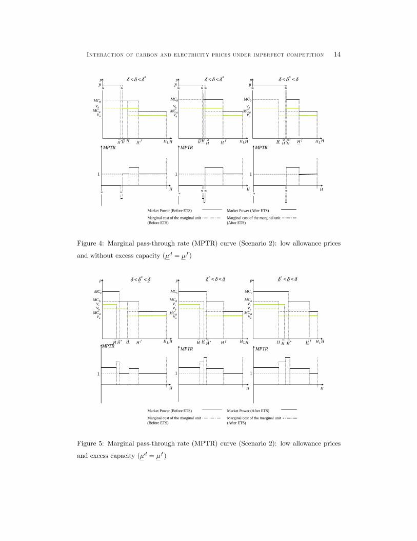
Interaction of carbon and electricity prices under imperfect competition 14
p
H LH HH~*~H
*δδδ <<
H HH
fH H
*δδδ <<p
H LH
δδδ << *
fH
p
HH LHH~~*~~H
fH
bMC
≈p
≈ ≈p p
≈
≈ ≈ ≈ ≈
≈ ≈≈
1 11
MPTR MPTR MPTR
≈ ≈ ≈
Market Power (Before ETS)
Marginal cost of the marginal unit(Before ETS)
Market Power (After ETS)
Marginal cost of the marginal unit(After ETS)
aMCbv
av
bMC
aMCbv
av
bMC
aMCbv
av
*~H H~~
Figure 4: Marginal pass-through rate (MPTR) curve (Scenario 2): low allowance prices
and without excess capacity (�d = �f )
p
H LH HH~ *~H
H HH
fH H
p
H LHfH
p
HH LHH~~ *~~H
fH
bMC
aMCbv
av
cv
cMC
δδδ << * δδδ <<*δδδ <<*
1 1 1
MPTR MPTR MPTR
bMC
aMCbv
av
cv
cMC
bMC
aMCbv
av
cv
cMC
Market Power (Before ETS)
Marginal cost of the marginal unit(Before ETS)
Market Power (After ETS)
Marginal cost of the marginal unit(After ETS)
H~ *~~H
Figure 5: Marginal pass-through rate (MPTR) curve (Scenario 2): low allowance prices
and excess capacity (�d = �f )
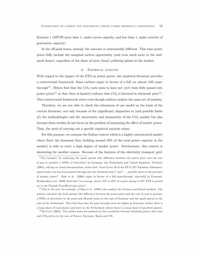
Interaction of carbon and electricity prices under imperfect competition 15
Scenario 1 (MPTR more than 1, under excess capacity, and less than 1, under scarcity of
generation capacity).
In the o¤-peak hours, instead, the outcome is substantially di¤erent. This time power
prices fully include the marginal carbon opportunity (and even much more in the mid-
merit hours), regardless of the share of most (least) polluting plants in the market.
3. Empirical analysis
With regard to the impact of the ETS on power prices, the empirical literature provides
a controversial framework. Some authors argue in favour of a full (or almost full) pass-
through14 . Others �nd that the CO2 costs seem to have not (yet) been fully passed into
power prices15 or that there is limited evidence that CO2 is factored in wholesale price16 .
This controversial framework arises even though authors analyse the same set of markets.
Therefore, we are not able to check the robustness of our model on the basis of the
current literature, not only because of the (signi�cant) disparities in (and possible limits
of) the methodologies and the uncertainty and immaturity of the CO2 market but also
because these studies do not focus on the problem of measuring the e¤ect of market power.
Thus, the need of carrying out a speci�c empirical analysis arises.
For this purpose, we examine the Italian context which is a highly concentrated market
where Enel, the dominant �rm (holding around 50% of the total power capacity in the
market) is able to exert a high degree of market power. Furthermore, this context is
interesting for another reason. Because of the features of the electricity transport grid,
14For instance, by analyzing the spark spread (the di¤erence between the power price and the cost
of gas to produce a MWh of electricity) in Germany, the Netherland and United Kingdom, Newbery
(2005), relying on visual interpretation, states that "most if not all of the EUA (EU Emission Allowance)
opportunity cost has been passed through into the wholesale price" and ".... possibly more in the presence
of market power". Sijm et al. (2006) argue in favour of a full pass-through, especially in Germany.
Honkatukia et al. (2006) �nd that "on average, about 75% to 95% of a price change in EU ETS is passed
on to the Finnish NoordPool spot price".15This is the case, for example, of Sijm et al. (2005) who analyze the German and Dutch markets. The
authors calculate the dark spread (the di¤erence between the power price and the cost of coal to produce
a MWh of electricity) in the peak and o¤-peak hours in the case of Germany and the spark spread in the
case of the Netherland. They �nd that that the pass through rates are higher in Germany (where there is
a large share of coal plants) and lower in the Netherland (where there is a large share of gas-�red plants).16See Levy (2005). The author bases his analysis on the correlation between wholesale prices, fuel costs
and CO2 prices in the case of France, Germany, Spain and UK.
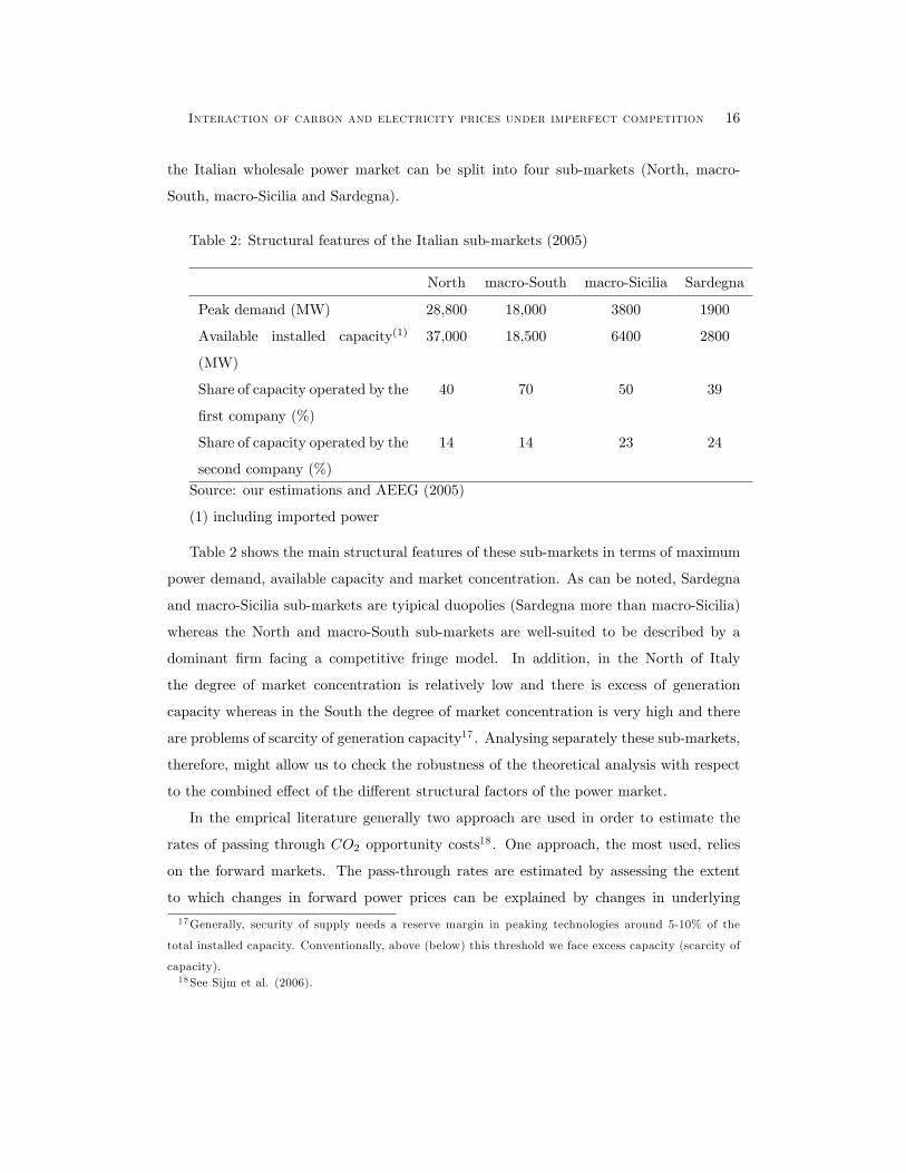
Interaction of carbon and electricity prices under imperfect competition 16
the Italian wholesale power market can be split into four sub-markets (North, macro-
South, macro-Sicilia and Sardegna).
Table 2: Structural features of the Italian sub-markets (2005)
North macro-South macro-Sicilia Sardegna
Peak demand (MW) 28,800 18,000 3800 1900
Available installed capacity(1)
(MW)
37,000 18,500 6400 2800
Share of capacity operated by the
�rst company (%)
40 70 50 39
Share of capacity operated by the
second company (%)
14 14 23 24
Source: our estimations and AEEG (2005)
(1) including imported power
Table 2 shows the main structural features of these sub-markets in terms of maximum
power demand, available capacity and market concentration. As can be noted, Sardegna
and macro-Sicilia sub-markets are tyipical duopolies (Sardegna more than macro-Sicilia)
whereas the North and macro-South sub-markets are well-suited to be described by a
dominant �rm facing a competitive fringe model. In addition, in the North of Italy
the degree of market concentration is relatively low and there is excess of generation
capacity whereas in the South the degree of market concentration is very high and there
are problems of scarcity of generation capacity17 . Analysing separately these sub-markets,
therefore, might allow us to check the robustness of the theoretical analysis with respect
to the combined e¤ect of the di¤erent structural factors of the power market.
In the emprical literature generally two approach are used in order to estimate the
rates of passing through CO2 opportunity costs18 . One approach, the most used, relies
on the forward markets. The pass-through rates are estimated by assessing the extent
to which changes in forward power prices can be explained by changes in underlying
17Generally, security of supply needs a reserve margin in peaking technologies around 5-10% of the
total installed capacity. Conventionally, above (below) this threshold we face excess capacity (scarcity of
capacity).18See Sijm et al. (2006).

Interaction of carbon and electricity prices under imperfect competition 17
forward prices for fuel and CO2 allowances. The other approach relies on spot markets by
comparing hourly electricity prices for the period after the ETS with the corresponding
hourly electricity prices in the period before the ETS (generally the year 2004).
Since in Italy currently there are not forward markets, we are obliged to use the
second approach which implicitily assumes that factors other than CO2 and fuel costs do
not change from 2004 to the subsequent years (2005 and 2006). According to this, the
di¤erence in the electricity price during a speci�c hour after the introduction of the ETS
and the corresponding hour in 2004 would be explained by the di¤erence in fuel prices
during the hours concerned, the impact of the CO2 price and by an error term19 .
Adopting this approach would imply that we should calculate the relevant spread (i.e.
the di¤erence between the electricity price and the cost of fuel to produce an unit of
electricity of the marginal plant) in the peak and o¤-peak hours (or in a particular hour
of the day) in every day of 2005 and 2006 and compare it with the corresponding spread
in 2004.
Nevertheless we think this way of proceeding might not be well-suited to our case, for
the following reason. It is based on the comparison of prices and spreads corresponding to
the same hour (or set of hours) in each day in di¤erent years under the implicit assumption
that the marginal technology (i.e. technology setting prices) does not vary from a year to
another on hourly basis. This hypothesis might be acceptable only if the demand level in
each hour does not change substantially from a year to another or if the power generating
system is characterised by low technological heterogeneity20 (i.e. a situation in which only
one kind of technology has a positive probability to become the marginal unit in most
hours, regardless of the power demand level).
Since this is very unlikely to occur, the time series approach (without appropriate and
complicated elaborations) may lead to incorrect interpretation. Consequently, it seems
more appropriate (and simple) reasoning in terms of load duration curves instead of time
series, i.e. directly comparing prices corresponding to similar levels of power demand
in di¤erent years. This approach, moreover, is consistent with the theoretical analysis
presented above.
19See Sijm et al. (2006).20This method is well suited to study markets where generation is mostly based on the use of a speci�c
fuel (like in Germany where power generation is mostly based on coal plants).
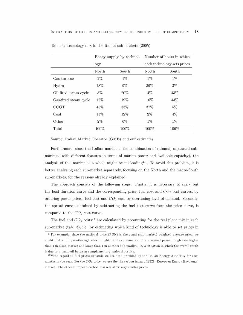
Interaction of carbon and electricity prices under imperfect competition 18
Table 3: Tecnology mix in the Italian sub-markets (2005)
Enegy supply by technol-
ogy
Number of hours in which
each technology sets prices
North South North South
Gas turbine 2% 1% 1% 1%
Hydro 18% 9% 39% 3%
Oil-�red steam cycle 8% 20% 4% 43%
Gas-�red steam cycle 12% 19% 16% 43%
CCGT 45% 33% 37% 5%
Coal 13% 12% 2% 4%
Other 2% 6% 1% 1%
Total 100% 100% 100% 100%
Source: Italian Market Operator (GME) and our estimates
Furthermore, since the Italian market is the combination of (almost) separated sub-
markets (with di¤erent features in terms of market power and available capacity), the
analysis of this market as a whole might be misleading21 . To avoid this problem, it is
better analysing each sub-market separately, focusing on the North and the macro-South
sub-markets, for the reasons already explained.
The approach consists of the following steps. Firstly, it is necessary to carry out
the load duration curve and the corresponding price, fuel cost and CO2 cost curves, by
ordering power prices, fuel cost and CO2 cost by decreasing level of demand. Secondly,
the spread curve, obtained by subtracting the fuel cost curve from the price curve, is
compared to the CO2 cost curve.
The fuel and CO2 costs22 are calculated by accounting for the real plant mix in each
sub-market (tab. 3), i.e. by estimating which kind of technology is able to set prices in
21For example, since the national price (PUN) is the zonal (sub-market) weighted average price, we
might �nd a full pass-through which might be the combination of a marginal pass-through rate higher
than 1 in a sub-market and lower than 1 in another sub-market, i.e. a situation in which the overall result
is due to a trade-o¤ between complementary regional results.22With regard to fuel prices dynamic we use data provided by the Italian Energy Authority for each
months in the year. For the CO2 price, we use the the carbon index of EEX (European Energy Exchange)
market. The other European carbon markets show very similar prices.
Interaction of carbon and electricity prices under imperfect competition 19
p
2H LH HH~ *~H
H
fH 2
ccMC
chpMCccv
chpv
gscv
gscMC
capacity)excess with;4.0(marketsubNorth
=δ
1
MPTR
H
capacityexcess without;7.0marketsubSouthMacro
=δp
HH LHH~~*~~H
fH
gscMC
gscv
≈p
≈
≈
1
MPTR
≈
oilMC
oilv
oilMC
oilv
1H fH1
plantscyclesteamfiredoiloilplants;cyclesteamfiredgasgscplants;cyclecombinedccplants;powerandheatcombinedchp:Note
====
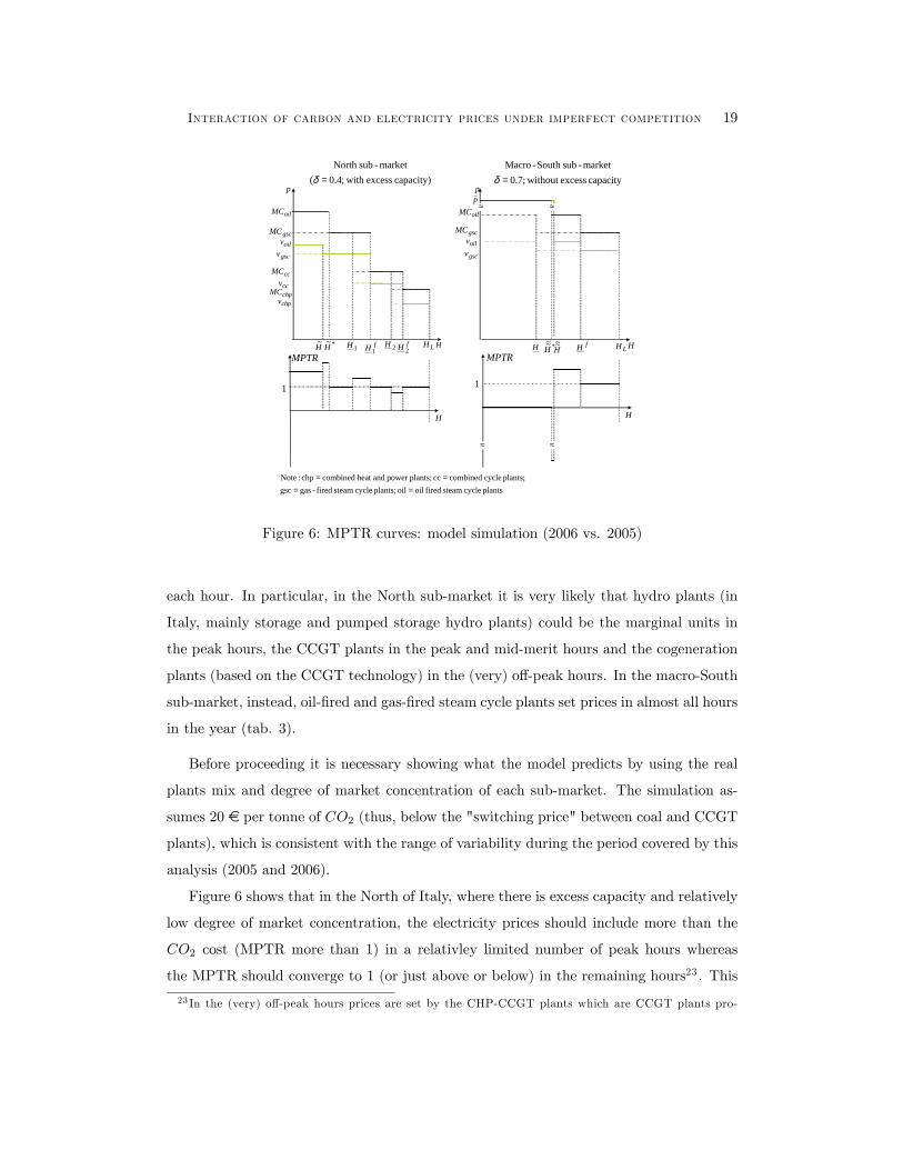
Figure 6: MPTR curves: model simulation (2006 vs. 2005)
each hour. In particular, in the North sub-market it is very likely that hydro plants (in
Italy, mainly storage and pumped storage hydro plants) could be the marginal units in
the peak hours, the CCGT plants in the peak and mid-merit hours and the cogeneration
plants (based on the CCGT technology) in the (very) o¤-peak hours. In the macro-South
sub-market, instead, oil-�red and gas-�red steam cycle plants set prices in almost all hours
in the year (tab. 3).
Before proceeding it is necessary showing what the model predicts by using the real
plants mix and degree of market concentration of each sub-market. The simulation as-
sumes 20 e per tonne of CO2 (thus, below the "switching price" between coal and CCGT
plants), which is consistent with the range of variability during the period covered by this
analysis (2005 and 2006).
Figure 6 shows that in the North of Italy, where there is excess capacity and relatively
low degree of market concentration, the electricity prices should include more than the
CO2 cost (MPTR more than 1) in a relativley limited number of peak hours whereas
the MPTR should converge to 1 (or just above or below) in the remaining hours23 . This
23 In the (very) o¤-peak hours prices are set by the CHP-CCGT plants which are CCGT plants pro-
Interaction of carbon and electricity prices under imperfect competition 20
North submarket
30
25
20
15
10
5
0
5
10
15
20
0 20 40 60 80 100
hours (%)
€/M
Wh
Change in spread
CO2 costs for gasfired steamcycle plants
CO2 costs for CCGT
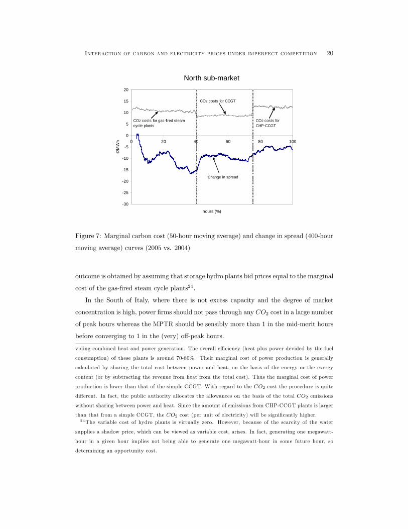
CO2 costs forCHPCCGT
Figure 7: Marginal carbon cost (50-hour moving average) and change in spread (400-hour
moving average) curves (2005 vs. 2004)
outcome is obtained by assuming that storage hydro plants bid prices equal to the marginal
cost of the gas-�red steam cycle plants24 .
In the South of Italy, where there is not excess capacity and the degree of market
concentration is high, power �rms should not pass through any CO2 cost in a large number
of peak hours whereas the MPTR should be sensibly more than 1 in the mid-merit hours
before converging to 1 in the (very) o¤-peak hours.
viding combined heat and power generation. The overall e¢ ciency (heat plus power devided by the fuel
consumption) of these plants is around 70-80%. Their marginal cost of power production is generally
calculated by sharing the total cost between power and heat, on the basis of the energy or the exergy
content (or by subtracting the revenue from heat from the total cost). Thus the marginal cost of power
production is lower than that of the simple CCGT. With regard to the CO2 cost the procedure is quite
di¤erent. In fact, the public authority allocates the allowances on the basis of the total CO2 emissions
without sharing between power and heat. Since the amount of emissions from CHP-CCGT plants is larger
than that from a simple CCGT, the CO2 cost (per unit of electricity) will be signi�cantly higher.24The variable cost of hydro plants is virtually zero. However, because of the scarcity of the water
supplies a shadow price, which can be viewed as variable cost, arises. In fact, generating one megawatt-
hour in a given hour implies not being able to generate one megawatt-hour in some future hour, so
determining an opportunity cost.
Interaction of carbon and electricity prices under imperfect competition 21
South submarket
30
25
20
15
10
5
0
5
10
15
20
0 20 40 60 80 100
hours (%)
€/M
Wh
Change in spread
CO2 cost for oil fired steam cycleplants
CO2 cost for gasfired steam cycleplants
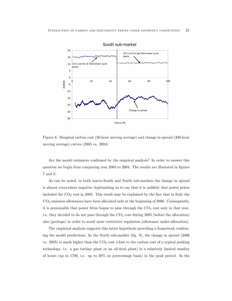
Figure 8: Marginal carbon cost (50-hour moving average) and change in spread (400-hour
moving average) curves (2005 vs. 2004)
Are the model estimates con�rmed by the emprical analysis? In order to answer this
question we begin from comparing year 2005 to 2004. The results are illustated in �gures
7 and 8.
As can be noted, in both macro-South and North sub-markets the change in spread
is almost everywhere negative, legitimating us to say that it is unlikely that power prices
included the CO2 cost in 2005. This result may be explained by the fact that in Italy the
CO2 emission allowances have been allocated only at the beginning of 2006. Consequently,
it is presumable that power �rms began to pass through the CO2 cost only in that year,
i.e. they decided to do not pass through the CO2 cost during 2005 (before the allocation)
also (perhaps) in order to avoid more restrictive regulation (allowance under-allocation).
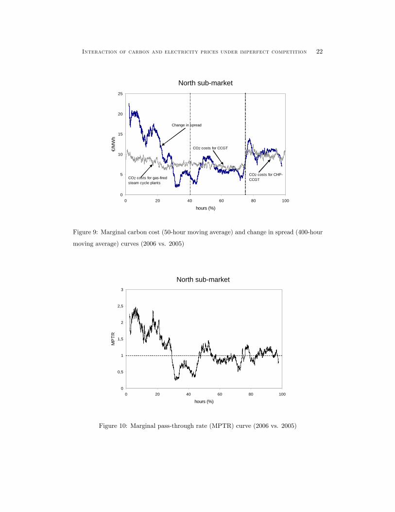
The empirical analysis supports this latter hypothesis providing a framework con�rm-
ing the model predictions. In the North sub-market (�g. 9), the change in spread (2006
vs. 2005) is much higher than the CO2 cost (close to the carbon cost of a typical peaking
technology, i.e. a gas turbine plant or an oil-�red plant) in a relatively limited number
of hours (up to 1700, i.e. up to 20% on perecentage basis) in the peak period. In the
Interaction of carbon and electricity prices under imperfect competition 22
North submarket
0
5
10
15
20
25
0 20 40 60 80 100
hours (%)
€/M
Wh
CO2 costs for gasfiredsteam cycle plants
CO2 costs for CCGT
CO2 costs for CHPCCGT
Change in spread
Figure 9: Marginal carbon cost (50-hour moving average) and change in spread (400-hour
moving average) curves (2006 vs. 2005)
North submarket
0
0,5
1
1,5
2
2,5
3
0 20 40 60 80 100
hours (%)
MP
TR
Figure 10: Marginal pass-through rate (MPTR) curve (2006 vs. 2005)
Interaction of carbon and electricity prices under imperfect competition 23
remaining hours the change in spread is more or less equal to the CO2 cost for the CCGT
and for CHP-CCGT. The shape of the MPTR curve, therefore, is enough similar to that
predicted by the model (�g. 10), except for the interval between 2200 and 4000 hours
(between 25% and 45% on pecentage basis). In this range, in fact, the model seems to
overestimate the pass-through rate25 .
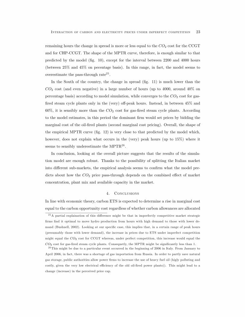
In the South of the country, the change in spread (�g. 11) is much lower than the
CO2 cost (and even negative) in a large number of hours (up to 4000, around 40% on
percentage basis) according to model simulation, while converges to the CO2 cost for gas-
�red steam cycle plants only in the (very) o¤-peak hours. Instead, in between 45% and
60%, it is sensibly more than the CO2 cost for gas-�red steam cycle plants. According
to the model estimates, in this period the dominant �rm would set prices by bidding the
marginal cost of the oil-�red plants (second marginal cost pricing). Overall, the shape of
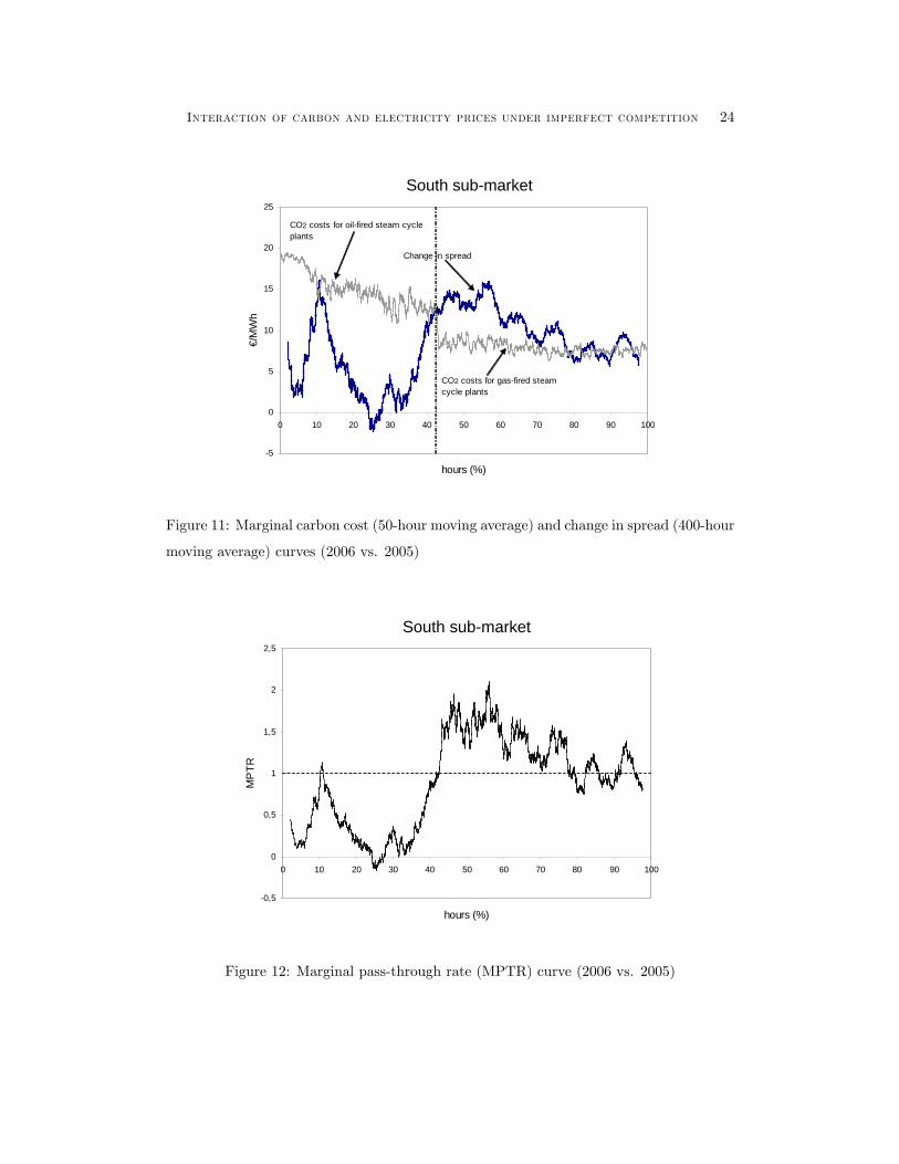
the empirical MPTR curve (�g. 12) is very close to that predicted by the model which,
however, does not explain what occurs in the (very) peak hours (up to 15%) where it
seems to sensibly underestimate the MPTR26 .
In conclusion, looking at the overall picture suggests that the results of the simula-
tion model are enough robust. Thanks to the possibility of splitting the Italian market
into di¤erent sub-markets, the empirical analysis seems to con�rm what the model pre-
dicts about how the CO2 price pass-through depends on the combined e¤ect of market
concentration, plant mix and available capacity in the market.
4. Conclusions
In line with economic theory, carbon ETS is expected to determine a rise in marginal cost
equal to the carbon opportunity cost regardless of whether carbon allowances are allocated
25A partial explaination of this di¤erence might be that in imperfectly competitive market strategic
�rms �nd it optimal to move hydro production from hours with high demand to those with lower de-
mand (Bushnell, 2002). Looking at our speci�c case, this implies that, in a certain range of peak hours
(presumably those with lower demand), the increase in prices due to ETS under imperfect competition
might equal the CO2 cost for CCGT whereas, under perfect competition, this increase would equal the
CO2 cost for gas-�red steam cycle plants. Consequetly, the MPTR might be signi�cantly less than 1.26This might be due to a particular event occurred in the beginning of 2006 in Italy. From January to
April 2006, in fact, there was a shortage of gas importation from Russia. In order to partly save natural
gas storage, public authorities allow power �rms to increase the use of heavy fuel oil (higly polluting and
costly, given the very low electrical e¢ ciency of the old oil-�red power plants)). This might lead to a
change (increase) in the perceived price cap.
Interaction of carbon and electricity prices under imperfect competition 24
South submarket
5
0
5
10
15
20
25
0 10 20 30 40 50 60 70 80 90 100
hours (%)
€/M
Wh
Change in spread
CO2 costs for oilfired steam cycleplants
CO2 costs for gasfired steamcycle plants
Figure 11: Marginal carbon cost (50-hour moving average) and change in spread (400-hour
moving average) curves (2006 vs. 2005)
South submarket
0,5
0
0,5
1
1,5
2
2,5
0 10 20 30 40 50 60 70 80 90 100
hours (%)
MP
TR
Figure 12: Marginal pass-through rate (MPTR) curve (2006 vs. 2005)
Interaction of carbon and electricity prices under imperfect competition 25
free of charge or not. Hence, common sense would suggest that �rms in imperfectly
competitive markets will pass-through into electricity prices only a part of the increase in
cost.
Instead, the theoretical analysis carried out in this paper shows that the result is
ambiguous. The increase in price can be, in fact, either lower or higher than the marginal
CO2 cost depending on several factors: (1) the degree of market concentration, (2) the
plant mix operated by either the dominant �rm or the competitive fringe, (3) the price
of the CO2 emissions allowances; (4) the available capacity in the market (whether there
is excess capacity or not). Furthermore the outcome substantially depends on the power
demand level, i.e. if we look at the peak or o¤-peak hours.
In the peak hours, the marginal pass-through rate (MPTR) is certainly less than 1
under scarcity of generation capacity whereas, under excess capacity, power prices include
the full marginal carbon opportunity cost (and even more).
In the o¤-peak hours the MPTR may be less than 1 only when there is "trade-o¤ in
the plant mix" (i.e. the technology with lower variable cost is the worse polluter, such as
in the case of coal plants vs. CCGT) and the share of most polluting plants is enough
high (regardless of whether there is excess capacity or not).
In order to check the robustness of the model estimates we have carried out an empirical
analysis of the Italian market, which is an emblematic case of imperfectly competitive
market. However, market power is asimmetrically distributed across the country. It is
relativley low in the North where, moreover, there are excess capacity and "trade-o¤ in
the plant mix". It is high in the South where, instead, there is scarcity of generation
capacity but not "trade-o¤ in the plants mix" (i.e. the technology with lower variable
cost is also the cleaner technology, such as in the case of gas �red vs. oil-�red steam cycle
plants).
By analysing separately these two sub-markets, we �nd results con�rming the model
predictions. In particular, in the North sub-market power prices include more than the
marginal CO2 cost in a relatively limited number of peak hours (up to the dominant �rm
prefers to use his relatively low market power). In the o¤-peak hours, the MPTR is equal
to 1 (or just below). In the macro-South sub-market, the marginal pass-through rate
is much lower than 1 (and even nil) for almost all the peak hours whereas power prices
include much more than the CO2 cost in o¤-peak hours (converging to the CO2 cost in
Interaction of carbon and electricity prices under imperfect competition 26
the very o¤-peak hours).
An overall picture, therefore, which seems to support the model simulations and sug-
gests the following consideration. Market power can really determines a deviation from
the "full pass-through" rule but we can not know which is the sign of this deviation,
a priori, i.e. without before carefully taking into account the structural features of the
power market.
5. Appendix
Proof of Lemma 1. It is immediately intuitive that when K � K the system
marginal price equals p (for Kc = 0) or MCc (for Kc = Kc). When K < Kf , pure
Bertrand equilibria (�rst marginal cost pricing) arise and prices equals the marginal cost of
the most e¢ cient plants (MC). In fact, on the one hand, whenever the demand is so high
that both leader�s and fringe�s least e¢ cient units can enter the market, the dominant �rm
would not gain any advantage by competing à la Bertrand, i.e. by attempting to undercut
the rivals. Therefore, he will maximize his pro�t by bidding the price threshold27 . On the
other hand, whenever the power demand is lower than the fringe�s power capacity in most
e¢ cient plants, competing à la Bertrand is the only leader�s available strategy in order
to have a positive probability of being dispatched. In consequence prices will converge to
the marginal cost of the most e¢ cient plants.
It remains to identify the leader�s optimal choice on K 2iK;Kf
i28 . Under the
assumptions of the model, each generator in the competitive fringe has a unique dominant
strategy whatever is the market demand: bidding according to its own marginal cost of
production (which, after the implementation of the ETS, includes the carbon opportunity
cost). By converse the best choice of the dominant �rm might consist in (1) bidding the
price cap (p, if there is not excess capacity, i.e. Kc = 0) or the backstop price (MCc, if
there is excess capacity, i.e. Kc = Kc) or in (2) bidding MC29 .
Let �d1 and �d2 be the pro�ts corresponding to the �rst and second strategies above,
27Strictly speaking, only o¤er prices of units that may become the marginal units (i.e. units belonging
to the group b) need equal the price cap or the backstop price.28Note that assuming a dominant �rm with competitive fringe model, rather than an oligopolistic
framework, assures that equilibria in pure-strategy do exist. For an explanation of why equilibria in pure
strategies do not exist in the case of oligopolistic competition, see von der Fehr and Harbord (1993).29Strictly speaking, bidding MC for units of kind b and p � MC � � (where � ' 0+) for units of kind
a.

Interaction of carbon and electricity prices under imperfect competition 27
respectively. Whenever the least e¢ cient units could enter the market (i.e. K(H) > K),
the pro�t the dominant �rm earns by choosing the �rst strategy (i.e. 8H 2�H;H
�) is
�d1 = (bp�MC) [K(H)�KH (1� �)]�Xz
i=1
Xj=a;b
�kijf
ij � ptpE
i
j
�(A1)
where f ij is the capital cost per unit of installed capacity of the unit i-th unit belonging
to the group j of plants and Ei
j the amount of allowance allocated (free of charge) to the
generic plant i belonging to the group j.
If the dominant �rm chooses the second strategy, he earns
�d2 =�MC �MC
��d�KH �
Xz
i=1
Xj=a;b
�kijf
ij � ptpE
i
j
�(A2)
where bp =8>><>>:p for Kc = 0
MCc for Kc = Kc
Therefore the leader�s optimal strategy is bidding bp if and only if �d1 � �d2, i.e. if andonly if
K ���d�� + (1� �)
�KH = eK(�; �d; �) (A3)
where � =
�MC �MC
�bp�MC
WhenK 2iK;Kf
i(i.e. H 2
iH;Hf
i) the pro�t the dominant �rm earns by choosing
the �rst strategy is
�d3 = (bp�MC) [K(H)�KH (1� �)]�Xz
i=1
Xj=a;b
�kijf
ij � ptpE
i
j
�(A4)
and by choosing the second strategy, the pro�t is
�d4 =�MC �MC
� �K(H)�KH�
f (1� �)��Xz
i=1
Xj=a;b
�kijf
ij � ptpE
i
j
�(A5)
Thus the dominant �rm will choose the �rst strategy (bidding the price cap or the
backstop price) if and only if �d3 � �d4; i.e. if and only if
K � (1� �)"(1� �f )(1� �) + �
f
#KH =
eeK(�; �f ; �) (A6)
Therefore the leader�s best reply is a function of power demand. We still have to demon-
strate that the two critical values eK and eeK never work together, i.e. if eK 2�K;K
�theneeK =2
iK;Kf
hand vice versa.
Interaction of carbon and electricity prices under imperfect competition 28
Given that Kf= (1 � �f )(1 � �)KH ; K
d = �d�KH ;Kf = (1 � �)KH and K =�
�d� + �f (1� �)�KH , equation (A3) can be rewritten as
K (H) � eK(�; �d; �) = �Kd +Kf (A7)
and equation (A6) as
K (H) � eeK(�; �f ; �) = Kf
1� � +Kf (A8)
Assume for instance eK > K. From (A7)Kf
(1� �) > Kd and from (A8) eeK > K: Thus,eeK =2
iK;Kf
h:
Similarly suppose eeK < K. From (A8) Kd >Kf
1� � and from (A7) eK < K. Thus,eK =2�K;K
�:
In addition, from (A7) and (A8), if eK = K then eeK = K and vice versa.
Finally, note that eK < K and eeK > Kf .
Last some comparative statics,
@ eK@�d
= ��KH > 0;@eeK
@�f= �(1� �) �
1� � KH < 0
In fact, when � > �; increasing fringe�s share of most e¢ cient plants implies that
bidding the marginal cost of the least e¢ cient plants becomes less pro�table for the
dominant �rm compared to bidding the price cap or the backstop price (�d4 in equation
(A5) decreases whereas �d3 in equation (A4) does not depend on �f ). Inversely when we
look at the case of � < � and at the rise of �d: This time increasing leader�s share of
most e¢ cient plants implies that bidding the marginal cost of the least e¢ cient plants
becomes more convenient for the dominant �rm (�d2 in equation (A2) increases whereas
�d1 in equation (A1) does not depend on �d). Furthermore,
@ eK@�
= �d�KH > 0;@eeK@�
=(1� �)(1� �f )
(1� �)2KH > 0
Thus, market power is a decreasing function of �.
5.1. Proof of Proposition 1. This proposition follows directly from Lemma 1. SinceeK and e~K never work together and provided that when eK = K then eeK = K (see the proof
Interaction of carbon and electricity prices under imperfect competition 29
of Lemma 1 above); in order to identify the critical value of � it su¢ ces carrying out the
locus of points of � (e�) that eK = K which is equal to the locus of points of � (ee�) thateeK = K e� = ee� = � = �f � 1�f � 1 + �d(� � 1)
Furthermore, note that eK < K and eeK > Kf .
5.2. Proof of Corollary 1. By di¤erentiating � with respect to ptp we get
@�
@ptp=
8>>><>>>:(eb � ea)(vc � va)� (ec � ea)(vb � va)
[(vc � va)� ptp(ec � ea)]2under excess capacity
(eb � ea)(p� va) + ea(vb � va)(p� va � ptpea)2
without excess capacity
Consequently,@�
@ptp< 0 when
8>>><>>>:(ec � ea)(vc � va)
>(eb � ea)(vb � va)
under excess capacity
�ea(p� va)
>(eb � ea)(vb � va)
without excess capacity
This condition always (never) is satis�ed when "trade-o¤ in the plant mix" combines
with excess capacity (without both "trade-o¤ in the plant mix" and excess capacity).
Since eK and eeK are increasing functions of � (see comparative statics in proof of Lemma
1 above), market power surely increases (decreases) in ptp when "trade-o¤ in the plant
mix" combines with excess capacity (without both "trade-o¤ in the plant mix" and excess
capacity). Otherwise, the ETS can determine either a rise or a decrease in market power
depending on the relative values of variable costs and emission rates of the di¤erent kinds
of technologies.
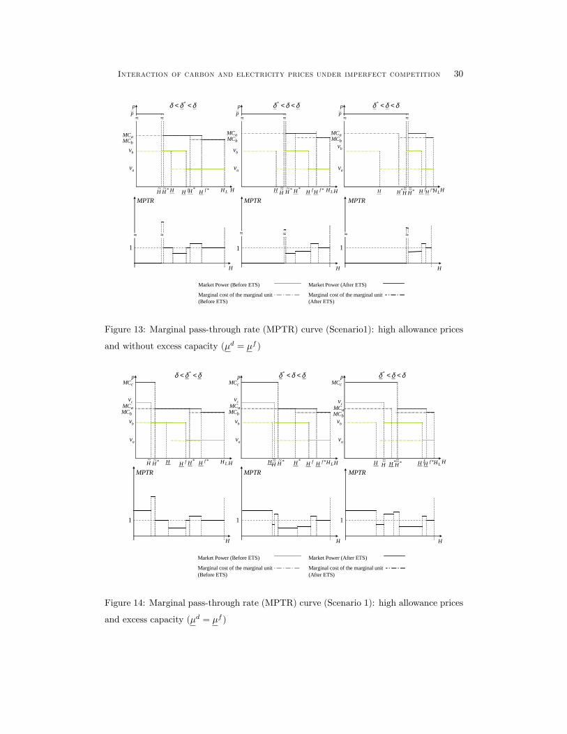
5.3. High allowance prices. For the sake of simplicity, we report only examples
referring to the Scenario 1. Figures 13 and 14 refer to an allowance price around 43
e/tonCO2, just above the "switching price" between coal and CCGT plants. As can
be noted, the outcome is very similar to that under low allowance prices (see subsection
2.3.)30 . This time, however, it is more likely that the MPTR could be less than 1 in the
o¤-peak hours.30As pointed out in note 11, explaining how the ETS can impact on market power under high allowance
prices is beyond the scope of this paper. However, it is possible to demontsrate that bK > bK� if the
allowance price is not very high (even if above the "switching price). This is the case simulated in �gs
A1 and A2.
Interaction of carbon and electricity prices under imperfect competition 30
pp
H LH*fH HH~ *~H
δδδ << *
H HH
≈ ≈ ≈
≈ ≈
fH *H H
δδδ <<*p
p
H LH*fHH~~ *~H
δδδ <<*
≈ ≈
fH*H
pp
≈ ≈
HH LH*fHH~~ *~~H
fH*H
Market Power (Before ETS)
Marginal cost of the marginal unit(Before ETS)
Market Power (After ETS)
Marginal cost of the marginal unit(After ETS)
1 11
MPTR MPTR MPTR
≈ ≈ ≈
bMCaMC
bv
av
bMCaMC
bv
av
bMCaMC
bv
av
Figure 13: Marginal pass-through rate (MPTR) curve (Scenario1): high allowance prices
and without excess capacity (�d = �f )
p
H LH*fH HH~ *~H
H H
MPTR
H
bMCaMC
fH *H H
p
H LH*fHH~~ *~H fH*H
p
HH LH*fHH~~ *~~H
fH*H
cMCδδδ << * δδδ <<*δδδ <<*
MPTR MPTR
1 11
Market Power (Before ETS)
Marginal cost of the marginal unit(Before ETS)
Market Power (After ETS)
Marginal cost of the marginal unit(After ETS)
bv
av
cv
bMCaMC
cMC
bv
av
cv
bMCaMC
cMC
bv
av
cv
Figure 14: Marginal pass-through rate (MPTR) curve (Scenario 1): high allowance prices
and excess capacity (�d = �f )
Interaction of carbon and electricity prices under imperfect competition 31
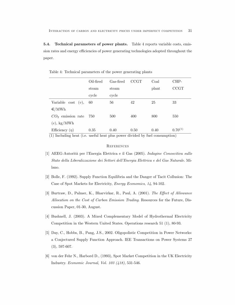
5.4. Technical parameters of power plants. Table 4 reports variable costs, emis-
sion rates and energy e¢ ciencies of power generating technologies adopted throughout the
paper.
Table 4: Technical parameters of the power generating plants
Oil-�red
steam
cycle
Gas-�red
steam
cycle
CCGT Coal
plant
CHP-
CCGT
Variable cost (v);
e/MWh
60 56 42 25 33
CO2 emission rate
(e); kg/MWh
750 500 400 800 550
E¢ ciency (�) 0.35 0.40 0.50 0.40 0.70(1)
(1) Including heat (i.e. useful heat plus power divided by fuel consumption)
References
[1] AEEG-Autorità per l�Energia Elettrica e il Gas (2005). Indagine Conoscitiva sullo
Stato della Liberalizzazione dei Settori dell�Energia Elettrica e del Gas Naturale. Mi-
lano.
[2] Bolle, F. (1992). Supply Function Equilibria and the Danger of Tacit Collusion: The
Case of Spot Markets for Electricity, Energy Economics, 14, 94-102.
[3] Burtraw, D., Palmer, K., Bharvirkar, R., Paul, A. (2001). The E¤ect of Allowance
Allocation on the Cost of Carbon Emission Trading. Resources for the Future, Dis-
cussion Paper, 01-30, August.
[4] Bushnell, J. (2003). A Mixed Complementary Model of Hydrothermal Electricity
Competition in the Western United States. Operations research 51 (1), 80-93.
[5] Day, C., Hobbs, B., Pang, J.S., 2002. Oligopolistic Competition in Power Networks:
a Conjectured Supply Function Approach. IEE Transactions on Power Systems 27
(3), 597-607.
[6] von der Fehr N., Harbord D., (1993), Spot Market Competition in the UK Electricity
Industry. Economic Journal, Vol. 103 (418), 531-546.
Interaction of carbon and electricity prices under imperfect competition 32
[7] von der Fehr, N., Harbord, D. (1998). Competition in Elecricity Spot markets - Eco-
nomic Theory and International Experience. Memorandum, n. 5, Department of Eco-
nomics, University of Oslo.
[8] Honkatukia, J., Malkonen, V., Perrels, A. (2006). Impacts of the European Emission
Trade System on Finnish Wholesale Electricity Prices. VATT Discussion papers 405.
[9] Hobbs, B., Rijkers, F. (2004a). Strategic Generation with Conjectured Transmission
Price Responses in a Mixed Transmission System I: Formulation. IEEE Transactions
on Power System, Vol. 19 (2), 707-717.
[10] Hobbs, B., Rijkers, F. (2004b). Strategic Generation with Conjectured Transmission
Price Responses in a Mixed Transmission System I: Application. IEEE Transactions
on Power System, Vol. 19 (2), 872-878.
[11] Honkatukia, J., Malkonen, V., Perrels, A. (2006). Impacts of the European Emission
Trade System on Finnish Wholesale Electricity Prices. VATT Discussion papers 405.
[12] Levy, C., (2005). Impact of Emission Trading on Power Prices. A case study from the
European Emission Trading Scheme. DEA d�Economie Industrielle, Université Paris
Dauphine, November.
[13] Lise, W. (2005). The European Electricity Market - What are the e¤ects of Market
Power on Prices and the Environment. Paper presented at EcoMod2005 International
Conference, ECN-RX-05-190, June 29 -July 2.
[14] Newbery, D. (2005). Emission Trading and the Impact on Electricity Prices. Mimeo.
14 December.
[15] Reinaud J. (2003). Emissions Trading and its Possible Impacts on Investment Deci-
sions in the Power Sector. IEA Information Paper.
[16] Requate, T. (2005). Environmental Policy under Imperfect Competition - A Survey.
CAU, Economics Working Papers, n. 2005-12.
[17] Sijm, J.P.M., Bakker, S.J.A., Chen, Y., Harmsen, H.W. (2005). CO2 Price Dynamics:
The Implications of EU Emissions Trading for the Price of Electricity. ECN Report,
ECN-C-05-081, September.
Interaction of carbon and electricity prices under imperfect competition 33
[18] Sijm, J., Neuho¤, K., Chen, Y. (2006). CO2 cost pass-through and windfall pro�ts
in the power sector. Climate Policy, 6, 49-72.
[19] Wals, A., Rijkers, F. (2003). How will a CO2 Price a¤ect the playing �eld in the
Northwest European Power Sector? ECN Report, September.
[20] Wolak, F. and Patrick, R. (1997). The Impact of Market Rules and Market Structure
on the Price Determination Process in the England and Wales Electricity Market.
Power Working Paper 047, University of California at Berkeley.