MPRAMunich Personal RePEc Archive

Federalism, decentralisation andcorruption

Sebastian Freille and Mohammad Emranul Haque and

Richard Anthony Kneller

Universidad Nacional de Cordoba, University of Manchester,University of Nottingham

June 2007

Online at https://mpra.ub.uni-muenchen.de/27535/MPRA Paper No. 27535, posted 21. December 2010 13:16 UTC

Federalism, decentralisation and

corruption

Sebastian Freille∗ M Haque Richard Kneller

June 2007

Abstract

We investigate the empirical relationship between decentralisation andcorruption. Using a newly assembled dataset containing data for up to 174countries, we revisit the empirical evidence and seek to explain some ofthe inconsistent results that exist in the literature. We find that not onlyresults differ due to the use of different specifications and data but moreimportantly because previous research overlooks the relationship betweendifferent dimensions of decentralisation. We propose an approach aimed atexploring the aggregate effect of decentralization on corruption. In this con-text, we analyze the existence of direct and indirect effects of these aspectson corruption. Our results suggest that fiscal (market) decentralisation isassociated with lower corruption. However, we also find that constitutionaldecentralisation (federalism) is associated with higher corruption. Further-more, we find that certain forms of political decentralisation worsen thepositive effect of constitutional centralization on corruption. Finally, otherforms of decentralisation such as spatial decentralisation do not appear tohave a strong association with corruption. Our results suggest the possi-bility that previous empirical work may grossly overestimate de aggregateimpact of decentralization and corruption.

Keywords: Fiscal decentralisation; Corruption; Federalism;Unitarism;Political institutions.

JEL Codes: H10, H40, H70, 01O

∗Room C36, University Park, University of Nottingham, NG7 2RD, Nottingham, UK.mailto:lexsf@nottingham.ac.uk

1

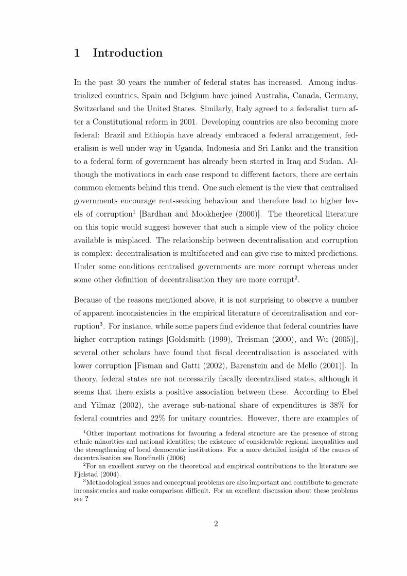
1 Introduction

In the past 30 years the number of federal states has increased. Among indus-

trialized countries, Spain and Belgium have joined Australia, Canada, Germany,

Switzerland and the United States. Similarly, Italy agreed to a federalist turn af-

ter a Constitutional reform in 2001. Developing countries are also becoming more

federal: Brazil and Ethiopia have already embraced a federal arrangement, fed-

eralism is well under way in Uganda, Indonesia and Sri Lanka and the transition

to a federal form of government has already been started in Iraq and Sudan. Al-

though the motivations in each case respond to different factors, there are certain

common elements behind this trend. One such element is the view that centralised

governments encourage rent-seeking behaviour and therefore lead to higher lev-

els of corruption1 [Bardhan and Mookherjee (2000)]. The theoretical literature

on this topic would suggest however that such a simple view of the policy choice

available is misplaced. The relationship between decentralisation and corruption

is complex: decentralisation is multifaceted and can give rise to mixed predictions.

Under some conditions centralised governments are more corrupt whereas under

some other definition of decentralisation they are more corrupt2.

Because of the reasons mentioned above, it is not surprising to observe a number

of apparent inconsistencies in the empirical literature of decentralisation and cor-

ruption3. For instance, while some papers find evidence that federal countries have

higher corruption ratings [Goldsmith (1999), Treisman (2000), and Wu (2005)],

several other scholars have found that fiscal decentralisation is associated with

lower corruption [Fisman and Gatti (2002), Barenstein and de Mello (2001)]. In

theory, federal states are not necessarily fiscally decentralised states, although it

seems that there exists a positive association between these. According to Ebel

and Yilmaz (2002), the average sub-national share of expenditures is 38% for

federal countries and 22% for unitary countries. However, there are examples of1Other important motivations for favouring a federal structure are the presence of strong

ethnic minorities and national identities; the existence of considerable regional inequalities andthe strengthening of local democratic institutions. For a more detailed insight of the causes ofdecentralisation see Rondinelli (2006)

2For an excellent survey on the theoretical and empirical contributions to the literature seeFjelstad (2004).

3Methodological issues and conceptual problems are also important and contribute to generateinconsistencies and make comparison difficult. For an excellent discussion about these problemssee ?

2

traditionally unitarist countries with a high degree of fiscal decentralisation. This

is the case of the Scandinavian nations where sub-national expenditures represent

over 30% of total government expenditures. The UK, embracing the devolved

state model, is another example with sub-national expenditures averaging 23%

during the 90’s. At the other end, certain federal countries have a low degree of

fiscal decentralisation: some notable examples are Croatia and Indonesia with only

around 10% of their total government expenditures accounted for by sub-national

governments.

Other studies focus on different aspects of decentralisation, such as political or ad-

ministrative decentralisation. Based on long-standing political science theories, it

has been argued that political decentralisation is important to improve account-

ability at the lower levels but the empirical evidence is inconclusive and often

contradictory. Among those who find that accountability is improved with the

existence of political decentralisation are Ames (1994) and Samuels (2000). Other

authors find no significant evidence of such relationship [Gelineau and Remmer

(2006)]. Additionally, some papers have found evidence that administrative de-

centralisation4 within the public sector is associated with lower corruption [Wade

(1997), Kuncoro (2004)].

In this paper we try to bring the empirics closer to the theory by acknowledging

the several different dimensions of decentralisation and by taking a closer look at

the empirical relationships among them. In so doing we build on a small recent

literature that recognises this point. Treisman (2002b,a) provides a systematic

treatment of the issue, carefully defining different types of decentralisation and

providing measures for each of them. Recognising the importance of their joint

effect on corruption he finds some direct effects but no interaction or indirect

effects. Our study has a closer relationship with Enikolopov and Zhuravskaya

(2007) however who test whether the effects of one of the aspects of decentralisation

we also consider, fiscal decentralisation, on corruption depend on the existence and

type of political institutions. In particular, they analyse how the level of political

centralisation modifies the effect of fiscal decentralisation on corruption. They

find evidence from this approach that strong party systems improve the result of

fiscal decentralisation on corruption and that political centralisation along with4On the field of administrative decentralisation, ?ścohen96 provide conceptual elements, high-

light links with other dimnesions and identify strategies of administrative decentralisation.

3

market decentralisation improves government quality for a sample of developing

countries. This evidence offers support for some long-standing political theories

of decentralisation.

Our work raises the following issues:

• Based on theoretical explanations, which decentralisation measures are im-

portant?

• Are there multi-dimensional aspects?

• Are there any significant interaction effects?

• What is the aggregate effect of decentralisation on bureaucratic corruption?

We contribute to this recent literature both by recognising and measuring the

existence of different dimensions of decentralisation but we also examine some

hypotheses in order to provide a sensible econometric model. We collect a large

set of decentralisation indicators -many of which have been used alternatively by

earlier research- and group them into categories in order to re-examine the rel-

evant empirical literature in a different light. Interestingly, we find evidence of

heterogeneity in the relationship between decentralisation and corruption regard-

less of the decentralisation measure used. Furthermore, unlike earlier research we

argue and find that some types of decentralisation are simultaneously associated

with corruption through both direct and indirect effects. We do not explore the

co-evolution of these dimensions of decentralisation5.

Our finding that long-standing unitary countries (constitutional centralisation)

which are also fiscally decentralised have low corruption is to some extent present

in earlier research. But unlike previous work, we find these two dimensions of

decentralisation significantly associated with corruption simultaneously. This re-

sult is quite robust both in terms of a variety of specifications and controls used

and in terms of alternative decentralisation measures. Furthermore, we also find5Unfortunately, we were not able to analyse time-varying features of the relationship between

corruption and decentralisation. Although we have data on corruption and other control variablessince 1975, there are almost no time-series data for decentralisation indicators. Apart fromannual dummies of no use in panel-data methods, the only decentralisation measures with time-series data are exp and rev. The problem with these is that the sample of countries sufferssignificant variations throughout the 25-year period.

4

evidence suggesting that political decentralisation -in particular, the existence of

municipal elections- is also associated to corruption but only indirectly through its

effect on constitutional decentralisation. In particular, political decentralisation

worsens the impact of constitutional centralisation on corruption. This result is

similar to Enikolopov and Zhuravskaya (2007) who find a negative indirect effect

of political institutions on corruption.

The remainder of the paper is organised as follows. In the next section, we review

the theoretical background of decentralisation and federalism, define the different

dimensions and explore the interrelations and overlaps between these dimensions.

Section 3 details the data and the empirical strategy followed. Section 4 presents

and discusses the main results. We also analyse different hypotheses regarding the

joint impact of different dimensions of decentralisation on corruption. Section 5

concludes.

2 Decentralisation and theory

To motivate the empirical analysis we provide a review of the literature on decen-

tralisation and corruption. Using a well-known approach6, we define four different

types of decentralisation.

Market Decentralisation7. Usually associated with the traditional theory of

fiscal federalism rooted in the public finance literature8, this form of decentrali-

sation is concerned with the study of the conditions required for the existence of

market mechanisms for the production and provision of goods and services. Based

on ideas developed during the 50’s, Oates (1972) shows first that in a multi-level

government situation where at least some public goods have regionally-bounded

benefits, decentralised finance provides opportunities for gains in social welfare.

Even in the presence of inter-jurisdictional externalities, decentralised provision

creates a better outcome as opposed to a uniform centralised provision of public6The categorisation follows loosely the Type-Function Framework. This is the currently

dominant approach to define and divide the different forms and types of decentralisation and islargely based on the work of Cheema, Nellis and Rondinelli. An overview of the Type-FunctionFramework given in ?

7In this paper, we use the terms market decentralisation and fiscal decentralisation indistinc-tively

8See Oates (2005) for references and summary of major contributions to this literature

5

goods. Second, there is an informational asymmetry: local governments are bet-

ter informed about the local preferences than the central government; this is also

known as the preference-matching argument for fiscal decentralisation. Third,

there is Tiebout’s ’voting-with-the-feet’ idea that citizens will sort themselves

into homogeneous communities demanding the same local public goods [Tiebout

(1956)]. Finally, the existence and enforcement of hard-budget constraints should

encourage local and regional governments to find ways to generate and rely on their

own sources of revenue. On the contrary, if the local and regional governments

customarily receive transfers from the centre or there are soft budget constraints,

it is likely that efficiency levels will drop. Taking these arguments together, we

would expect the scope for bureaucratic corruption to be lower in the presence

of market decentralisation. In principle, intergovernmental competition to attract

residents lowers the incentive and ability to extract rents and bribes. Moreover,

the existence of hard-budget constraints reduces the scope for corruption since

local governments are entirely responsible for financing their own expenditures.

In spite of the previous considerations, there remain theoretical arguments that

suggest that forms of market decentralisation, such as fiscal decentralisation, may

create perverse incentives and stimulate corrupt behaviour. For example, because

of over-budgeting and lack of accountability in the case of soft-budget constraints

arising from tax evasion and unconditional intergovernmental grants. This situa-

tion may be particularly relevant in cases where there is no political decentralisa-

tion. Another possible factor that may distort incentives is the way sub-national

budgets are financed. Barenstein and de Mello (2001) have suggested that the re-

lationship of fiscal decentralisation to corruption hinged on the way sub-national

expenditures are financed.

Political Decentralisation. There is perhaps no better description of the dif-

ficulties in defining centralisation than Alexis de Tocqueville’s observation that

“Centralisation is now a word constantly repeated but is one that, generally speak-

ing, no one tries to define accurately”9. Alongside Montesquieu and philosophers

from the Enlightenment, de Tocqueville’s ideas on federalism and decentralisation

generated vigorous research effort to study the advantages and disadvantages of

political decentralisation. The central idea of political decentralisation (or gov-9Alexis de Tocqueville, Democracy in America, Vol. 1, Part 1, ch. 5.

6

ernment decentralisation as is also called) is that citizens should be given more

power in political and public decision-making. This involves the creation of a

number of different institutions that support this objective. Local and regional

elections, regional autonomy, local committees and civil associations, sub-national

authority over taxation, spending and legislation, are all different mechanisms in-

volved in the context of political decentralisation. There are several arguments

favouring political decentralisation. The most commonly cited are the greater ac-

countability to the local and regional electorate, the development of a civic local

culture by fostering democratisation and the involvement of other local actors in

the decision-making process (NGO’s, civil and professional associations, private

sector, etc.).

Despite these theoretical arguments endorsing political decentralisation, others

have highlighted the potential dangers associated to political decentralisation.

One of the most notable contributions is the work of Riker (1964), who pro-

vided strong theoretical arguments in favour of political centralisation. The basic

idea is that political centralisation may serve as a mechanism to complement and

boost the outcome of fiscal decentralisation by making local politicians internalise

inter-jurisdictional externalities to a greater extent. Alternatively Bardhan and

Mookherjee (2000) argue that political decentralisation may not be as effective if

local capture of public officials by interest groups is widespread.

Constitutional Decentralisation10. The concept of constitutional decentrali-

sation (or equivalently constitutional federalism) is closely associated with what is

known as de iure federalism, representing the establishment of a federal regime by

the Constitution. There is however, in addition the concept of contingent decen-

tralisation, which refers to our current understanding of federalism as including

the erosion and degradation of the constitutional decentralisation principle by

jurisprudence and/or Courts rulings [Aranson (1990)]. In words of this author,

“Federalism as constitutional decentralisation differs from federalism as contingent

decentralisation in that the authority of the states under constitutional decentrali-

sation is guaranteed as a matter of organic, constitutional law. Neither prudential

nor political judgments or decisions taken at the national level can overturn such10We refer to constitutional decentralisation as the Constitution’s federalism, the legal doc-

trine. This expression was originally introduced by Diamond (1969) in his article about therelationship between federalism and decentralisation.

7

guarantees in the face of the appropriate legal fidelity to the original constitu-

tional arrangement” [Aranson (1990), p. 20]. One connotation derived from this

distinction is that constitutional decentralisation is a rather static concept while

contingent decentralisation is inherently dynamic. In general, constitutional and

contingent decentralisation will differ: contingent decentralisation is driven by

pure utilitarist motives and this will shape the distribution of powers and federal

arrangements in practice. Aranson (1990) shows the widening gap between these

two concepts but in general it has happened in several other federal countries.

It may be even argued that contingent decentralisation will eventually cause a

country to re-centralize if many judicial or consuetudinary instances erode the

true nature and spirit of constitutional decentralisation. At the empirical level,

however, distinguishing between these two types of ’federalism’ is not practicable

and only constitutional decentralisation measures can be used.

What are the predictions of the theory for the relationship between constitutional

decentralisation and corruption? Similarly to the case of political decentralisation

the answer is not clear. Constitutional federalism has often been advocated as a

system to accommodate ethnic and religious differences and other regional diver-

gences [Bermeo (2002)]. Federalism provides room for diversity and reduces the

possibility of tensions and conflicts which may also originate opportunities for the

extraction of rents. Yet on the other hand, the well-known arguments of multi-

plication and overlapping of layers of government causing accountability problems

and the ’overgrazing’ of the bribe base in federal systems suggests that the latter

may also be associated to higher corruption.

Spatial Decentralisation. This form of decentralisation refers to the actions

and strategies aimed at encouraging the development of regional growth poles

outside major urban areas. If succesful, this has obvious implications for the

distribution of the size of cities. In political economy, it is usually associated

with a narrower concept and known as structural or vertical decentralisation. For

example Treisman (2002b) suggests that structural decentralisation refers to the

number of tiers of government. Essentially, the greater the number of tiers the

more decentralised a country is. This definition gives only a partial and crude

account of this type of decentralisation as it only considers the number of levels

of government and not the number, size and density of cities.

8

Spatial decentralisation is likely to be related to other forms of decentralisation,

most evidently with constitutional decentralisation. In fact, it is possible that

with several tiers of government, only some may have the constitutional authority

over certain decisions (i.e. spending, taxing, legislation, etc.) or be responsible for

their own sources of revenues and expenditures. The definition given by Treisman

defines a tier as having a political executive in charge of certain decisions over a

territorial jurisdiction. It is also clear from this that spatial and political decen-

tralisation may be closely linked. Other measures, including the number of cities

at the intermediate and local level, may be also considered as representing aspects

of spatial decentralisation.

3 Data and sample characteristics

The empirical approach adopted in the paper builds the relationship between

decentralisation in stages. In the first stage we try to identify which measures of

the different aspects of decentralisation are correlated with corruption. As a second

stage we then consider the multi-faceted nature of decentralisation, and attempt

to establish the robustness of the results in the first stage to other aspects of

decentralisation. Finally, we allow for the possibility that there may be interesting

interactions between the various measures of decentralisation.

In this section we describe and motivate the choice of regression model that we use

in the first stage of the empirical analysis and summarise the main characteristics

of the data. The baseline model we adopt in the paper is given by a standard

corruption equation. It regresses a measure of corruption against a series of control

variables usually included in any corruption regression [Treisman (2000); Serra

(2006)] and a series of decentralisation measures:

CORRi = β0 + β1DECi + β2 logGDPi + β3 logPOPULi + β4PRESSi + εi (1)

where CORRi is the corruption index of choice, DECi is our decentralisation

indicator, logGDPi is the logarithm of GDP per capita (PPP), logPOPULi is the

9

logarithm of total population and PRESSi is the degree of press freedom11.

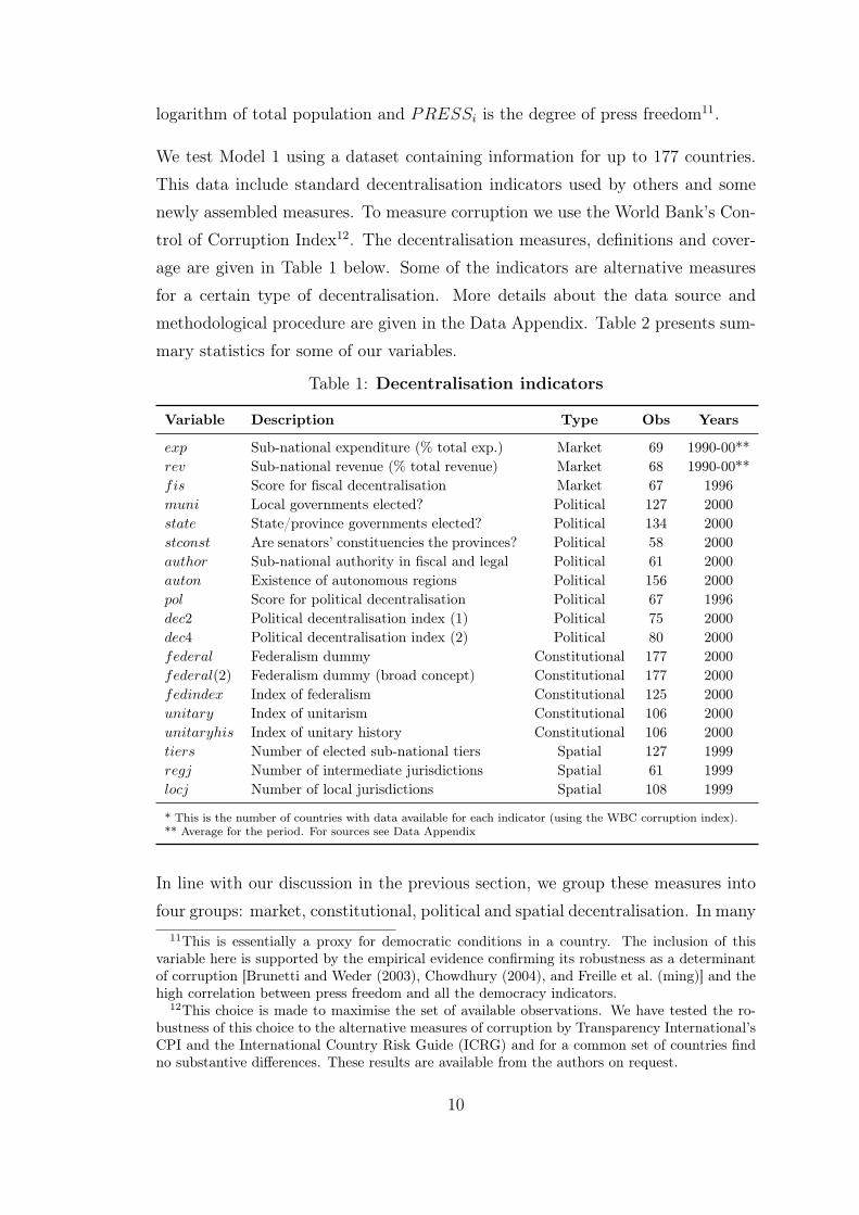
We test Model 1 using a dataset containing information for up to 177 countries.

This data include standard decentralisation indicators used by others and some

newly assembled measures. To measure corruption we use the World Bank’s Con-

trol of Corruption Index12. The decentralisation measures, definitions and cover-

age are given in Table 1 below. Some of the indicators are alternative measures

for a certain type of decentralisation. More details about the data source and

methodological procedure are given in the Data Appendix. Table 2 presents sum-

mary statistics for some of our variables.

Table 1: Decentralisation indicators

Variable Description Type Obs Years

exp Sub-national expenditure (% total exp.) Market 69 1990-00**rev Sub-national revenue (% total revenue) Market 68 1990-00**fis Score for fiscal decentralisation Market 67 1996muni Local governments elected? Political 127 2000state State/province governments elected? Political 134 2000stconst Are senators’ constituencies the provinces? Political 58 2000author Sub-national authority in fiscal and legal Political 61 2000auton Existence of autonomous regions Political 156 2000pol Score for political decentralisation Political 67 1996dec2 Political decentralisation index (1) Political 75 2000dec4 Political decentralisation index (2) Political 80 2000federal Federalism dummy Constitutional 177 2000federal(2) Federalism dummy (broad concept) Constitutional 177 2000fedindex Index of federalism Constitutional 125 2000unitary Index of unitarism Constitutional 106 2000unitaryhis Index of unitary history Constitutional 106 2000tiers Number of elected sub-national tiers Spatial 127 1999regj Number of intermediate jurisdictions Spatial 61 1999locj Number of local jurisdictions Spatial 108 1999

* This is the number of countries with data available for each indicator (using the WBC corruption index).** Average for the period. For sources see Data Appendix

In line with our discussion in the previous section, we group these measures into

four groups: market, constitutional, political and spatial decentralisation. In many11This is essentially a proxy for democratic conditions in a country. The inclusion of this

variable here is supported by the empirical evidence confirming its robustness as a determinantof corruption [Brunetti and Weder (2003), Chowdhury (2004), and Freille et al. (ming)] and thehigh correlation between press freedom and all the democracy indicators.

12This choice is made to maximise the set of available observations. We have tested the ro-bustness of this choice to the alternative measures of corruption by Transparency International’sCPI and the International Country Risk Guide (ICRG) and for a common set of countries findno substantive differences. These results are available from the authors on request.

10

cases we can capture different aspects of these four main types of decentralisation.

We detail the data sources for these variables in the Appendix, along with some

summary statistics and the correlation between the variables.

Fiscal Decentralisation. The most commonly used indicator of fiscal decen-

tralisation in the literature is the percentage ratio of sub-national government

expenditure to total government expenditure. We also consider the sub-national

government revenue since it is also a reasonable measure13. In both cases the data

are an average for the 1990-2000 period.

Constitutional Decentralisation. Constitutional decentralisation refers to whether

the structure of the relations between different government units are based on fed-

eral or unitary grounds according to legal bodies. In general, researchers capture

this as a zero-one dummy with all countries not explicitly federal being considered

as unitarian. In our study we explore several alternatives to this. Our main control

for the federal structure of a country -unitaryhis-, however, is a newly assembled

indicator that measures not only the current status of federal or unitary but also

takes into account history into consideration. In particular, this variable gives the

score of unitary history for a country during a period of 100 years. In other words,

if a country has always been a federation or federal (Argentina, Canada, Malaysia

and Switzerland among others), then the score assigned is 0. Countries that have

been mostly unitary throughout this time period (like Denmark, Japan, and Swe-

den), receive high scores, whereas countries that have changed either changed

regime or have a relatively short unitary history are ranked in between (Austria,

Spain and Thailand).

Political Decentralisation. According to the World Bank, political decentrali-

sation is about providing the citizens of a country more power in public decision-

making and is associated with institutions ranging from pluralistic politics and

representative government, to local and regional democratization and greater par-

ticipation in decisions. We have a number of political decentralisation indicators

taken from different sources. We consider three of these to most fully capture13One problem of using these two indicators as alternative is the existence of vertical fiscal im-

balances. In short, this implies that sub-national revenues fall short of sub-national expenditureand the difference should be compensated by coordination mechanisms between the different lev-els of government. If the vertical imbalance is relatively high, it is better to use the expenditureindicator since it captures more adequately the degree of public service decentralisation.

11

Table 2: Summary statistics for selected variablesVariable Description Mean Std. Dev. Min. Max. Nexp Share of sub-national gov. exp. 22.9 15.6 2.02 80.53 69rev Share of sub-national gov. revenue 18.03 14.8 0.81 78.12 68author Sub-national authority in spend/tax 0.44 0.5 0 1 61federal_alt Dummy for federalism [Treisman] 0.1 0.3 0 1 177tiers Number of elected sub-national tiers 1.16 0.89 0 3 127regj Number of intermediate jurisdictions 26.74 24.9 2 135 61locj Number of local jurisdictions 4438.56 23949.3 17 237687 108muni Local governments elected? 1.36 0.82 0 2 127state State/prov. governments elected? 0.87 0.81 0 2 134fis Score for fiscal decentralisation 0.41 0.22 0 1 67pol Score for political decentralisation 0.55 0.23 0 1 67adm Score for adm. decentralisation 0.54 0.28 0.01 1 67auton Existence of autonomous regions? 0.1 0.3 0 1 156stconst Are senators’ constituencies the

provinces?0.5 0.5 0 1 58

dec2 Political decentralisation index 1 2.21 1.6 0 5 75dec4 Political decentralisation index 2 2.2 1.53 0 4 80federal Dummy for federal countries 0.13 0.34 0 1 177fedindex Index of federalism 4.14 1.32 1 5 125unitary Index of unitarism 1.6 0.74 0 2 106unitaryhis Index of unitary history 36.82 31 0 101 106federal(2) Federal dummy (broad) 0.28 0.45 0 1 174cpi Corruption Perception Index (TI) 4.73 2.4 1.2 10 91icrg Corruption Index (ICRG) 2.96 1.22 1 6 140wbc Corruption Index (World Bank) -0.02 1.03 -1.8 2.5 173loggdp Log of GDP per capita 3.68 0.51 2.67 4.77 160logpopul Log of total population 6.86 0.76 5.01 9.1 174pss Press freedom index 48.17 25.04 5 100 174democindex Index of democracy 5.93 7.99 0 66 153demochis Dummy for democratic history 0.26 0.44 0 1 107polrights Index of political rights 3.59 2.23 1 7 174democ1 Alternative democracy index 3.65 1.98 1 7 174bri Dummy for former British colony 0.28 0.45 0 1 177fre Dummy for former French colony 0.16 0.37 0 1 177spa Dummy for former Spanish colony 0.11 0.32 0 1 177por Dummy for former Port. colony 0.03 0.17 0 1 177ethno Ethno-linguistic frac. index 0.35 0.3 0 1 143eng English legal system (dummy) 0.31 0.46 0 1 175soc Socialist legal system (dummy) 0.19 0.4 0 1 175fre French legal system (dummy) 0.43 0.5 0 1 175ger German legal system (dummy) 0.03 0.18 0 1 175sca Scandinavian legal system (dummy) 0.03 0.17 0 1 175pro_d Dummy for Protestant country 0.22 0.41 0 1 174Note: Only selected variables are given in the Table. Data for year 2000, otherwise the closest availableyear. For sources and data description see table 11 in Appendix ??

12

the essence of political decentralisation: muni, a categorical variable indicating

the existence of municipal executive and legislative elections, state, a similar vari-

able for provincial or state elections and stconst, a dummy registering whether

the provinces/states represent the constituencies of the senators. Although we

consider all three indicators in our regressions, we believe the variables measur-

ing the existence of municipal elections, muni, best captures the idea of political

decentralisation.

Spatial Decentralisation. Finally, spatial decentralisation concerns the vertical

(number of tiers) and horizontal (number of jurisdictions within each tier) make-

up of the political structure14. We use three indicators: the number of elected

tiers (tiers), the number of elected regions or jurisdictions within the upper tier

(regj ) and the number of elected localities or jurisdictions within the lower tier

(locj ).

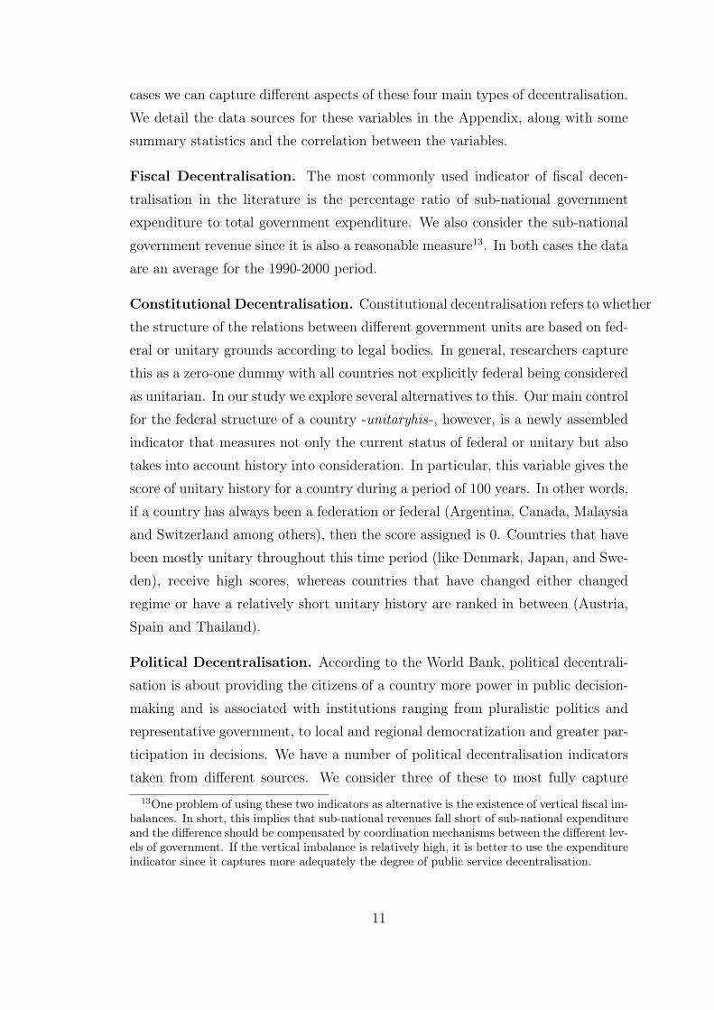
Table 8 in the Appendix shows the correlations between different forms of de-

centralisation, while we reproduce the correlation from the main decentralisation

variables in Table 3. It appears from both that the interrelations between con-

stitutional, political and structural decentralisation are straightforward. Of the

correlations that are found some are intuitive; the positive correlation between

federal and unitaryhis ; that countries with a federal system are also likely to have

local (muni) and regional (state) elections and have higher number of elected gov-

ernment tiers (tiers), for example. Other significant correlations are harder to

explain as is the case with the correlation between unitaryhis and stconst.

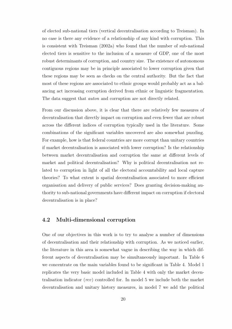
Figure 1 provides a different way to look at the data. Here we arrange countries

according to their fiscal and constitutional decentralisation regimes and indicate

the level of corruption in those countries. According to the previous literature,

we would expect countries with a high level of market decentralisation and with

constitutional centralisation (unitarism) to show low corruption levels. This is

observerd in the figure by looking at the upper right-hand side quadrant where all

countries (in bold) have low corruption levels. Similarly, countries with low levels

of market decentralisation and with constitutional decentralisation (federalism)

should have high corruption levels. Although the evidence is not as strong as14Treisman (2002b) introduces his definition of vertical decentralisation by measuring the

number of tiers in a system. This categorization includes single-tiered systems such as Singaporeand multi-tiered systems such as Argentina, the United States and China.

13

Table 3: Pairwise correlations between selected decentralisation indica-tors

Variables unitaryhis muni locj federal state stconst tiers regj

unitaryhis 1.000(106)

muni 0.137 1.000(85) (127)

locj -0.141 0.108 1.000(78) (90) (216)

federal -0.330* 0.209* 0.275* 1.000(106) (127) (216) (177)

state 0.045 0.547* 0.066 0.361* 1.000(84) (110) (96) (134) (134)

stconst -0.318* 0.314* 0.201 0.447* 0.288* 1.000(48) (45) (41) (58) (49) (58)

tiers 0.140 0.479* 0.190* 0.437* 0.359* 0.463* 1.000(81) (104) (108) (127) (107) (42) (127)

regj 0.085 0.112 -0.003 -0.138 0.004 -0.150 0.005 1.000(47) (55) (60) (61) (53) (31) (61) (61)

Notes: The number of observations is given under the corresponding correlation. * Denotes significanceat the 10% level

in the previous case, the lower left-hand side quadrant shows most countries as

having intermediate to high corruption levels.

4 Fiscal decentralisation, federalism and political

institutions

4.1 Which aspects of decentralization matter?

Tables 4 and 5 contain the results for the baseline regression specified above. We

have considered the robustness of the results to alternative measures of corruption

(the CPI and ICRG indices of corruption) and to changes in the number of ob-

servations. We also reproduce the latter in Table 9 in the Appendix ?? where we

use a common subset of countries including all the countries with data available

for all three corruption indexes.

14

Figure 1: Fiscal and constitutional decentralisation

In discussing the results we begin with the market decentralisation indicators, the

sub-national government expenditure as a percentage of total government expen-

diture and sub-national government revenue as a percentage of total government

revenue. The results for these variables are consistent with earlier research: fis-

cal decentralisation is associated with lower corruption ratings [Huther and Shah

(1998); Fisman and Gatti (2002); Barenstein and de Mello (2001)]. The coeffi-

cients are also similar in size to those obtained previously.

In contrast to the results for market decentralisation less agreement has been found

in the literature for constitutional decentralisation. Treisman (2000) found that

federal states are perceived to be more corrupt and that this conclusion was robust

to several tests, whereas for a different indicator Gerring et al. (2005) find that

unitary systems are strongly associated to good governance. Other have found

no relationship between federalism and corruption [Fisman and Gatti (2002); Wu

(2005)].

Table 5 confirms these mixed results. The zero-one federal dummy suggests that

federalism has no relationship with corruption, a result similar to that obtained if

15

we use the federal dummy included in Treisman (2000)15. Investigating the results

further, we find that we are unable to replicate Treisman’s result that federal states

are more corrupt for two reasons. Firstly, the effect of the federalism dummy is

sensitive to the inclusion of the logarithm of total population and to cultural and

historical indicators. Second, the results for the federalism dummy are sensitive

to the year of choice. Specifying the model and the data as closely as possible to

Treisman, our results are similar to his paper for 1996 and 1998 (federal states are

more corrupt) although the coefficients are never significant, but the coefficients

become negative when we use either 2000 or 2002 (federal states are less corrupt).

Also in Table 4 we explore whether using more detailed measures of constitutional

decentralisation help to improve the robustness of this variable. The first mea-

sure is an index of federalism (fedindex) ranging from 1 (most federal) to 5 (most

unitary). Although the positive sign of the coefficient implies that unitary coun-

tries are associated to lower corruption levels, it is not significantly different from

zero. The second measure is taken from Gerring et al. (2005). The authors study

the relative merits of federal and unitary systems and come to the conclusion that

long-standing unitary systems are associated with lower corruption. The unitarism

index (unitary) takes values of 0=federal (elective regional legislatures plus con-

stitutional recognition of sub-national authority), 1=semi-federal (where there are

elective legislatures at the regional level enjoying important policymaking power

but in which constitutional sovereignty is reserved to the national government),

and 2=unitary [Gerring et al. (2005)]. As it can be observed from Table 5, the

coefficient on this variable is again not significant.

Our final indicator, also from Gerring et al. (2005), is an index of unitary history

(unitaryhis) created on the basis of the annual unitary scores used to construct the

dummy unitary16. The estimation results (regression corresponding to unitaryhis

in Table 4) show that countries with long standing unitary regimes perform better15Our federal dummy includes a slightly larger number of countries and therefore the number

of federal states differ between our study and Treisman’s. He uses the classification of federalcountries as given in Elazar (1995), while we use this and other sources to update the data. Asa result of this, we add Bosnia and Herzegovina, Comoros, Ethiopia, Serbia and Montenegro,South Africa, and the United Arab Emirates to the list of federal countries.

16Although the authors have used time series data we estimate the model using the indexfor the year 2000. We do this since there is little year-to-year variation in the index and wewere unable to obtain the original data. The variable measures the unitary history of a countryfrom 1901 to 2000. For construction, measurement and coverage of this index see Gerring et al.(2005).

16

in terms of corruption. Using our simple baseline regression, we have obtained the

same qualitative results as Gerring et al. (2005), although it should be noted that

they use the ICRG index of corruption instead. For the same index of corruption

we find an insignificant effect from the unitary history variable (it is significant if

we use the CPI index of corruption)17.

In other models in Tables 4 and 5, we explore the relationship between political

dimensions of decentralisation and corruption. Several forms of political decen-

tralisation have been recognized in the literature including electoral decentralisa-

tion, structure of the party system, decision-making authority and residual powers

[Treisman (2002b,a); Enikolopov and Zhuravskaya (2007)]. We focus, however, on

a subset of these aspects for which we can find reliable data, namely indicators

of electoral and authority decentralisation (also known as decision-making decen-

tralisation).

It can be seen from Table 4 that none of the indicators of political decentralisation

are significantly and consistently correlated to perceived corruption. Table 5 in

Appendix suggests that this results is not robust for all measures of corruption

however. According to the regression, the variable author the greater the authority

over spending, taxing and legislation that is granted to sub-national governments,

the more likely corrupt behaviour will arise when we measure corruption using

the ICRG index. While the existence of municipal/local elections at executive

and legislative level -muni - is negatively associated with the CPI measure of cor-

ruption, along with an aggregate indicator of political decentralisation, dec4, which

aggregates over muni and state. The sensitivity of the political decentralisation

measures as determinants of corruption matches results found elsewhere in the

literature [Treisman (2002b,a)]. Enikolopov and Zhuravskaya (2007) find no di-

rect relation of these indicators to corruption (only through their interaction with

fiscal decentralisation measures)18.

Finally in Table 4 we direct our attention to the spatial decentralisation indicators.

The existence of autonomous contiguous regions, the number of regional jurisdic-

tions and the number of local jurisdictions are included here along with the number17Some investigation suggests that this difference is due to the use of panel data in their study.18The severe limitations of the data, in its majority dummies or categorical variables suggest

a careful interpretation of these findings. In any case, the available indicators do not seem to beaffecting or affected by corruption in a direct way.

17

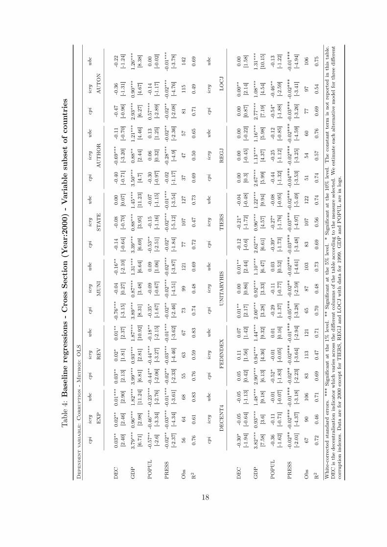
Table4:

Baselineregression

s-Cross

Section

(Year:20

00)-Variable

subsetof

countries

Dep

enden

tva

ria

ble:

Corru

ptio

n-

Met

hod:

OLS

cpi

icrg

wbc

cpi

icrg

wbc

cpi

icrg

wbc

cpi

icrg

wbc

cpi

icrg

wbc

cpi

icrg

wbc

EXP

REV

MUNI

STATE

AUTHOR

AUTON

DEC

0.03

∗∗0.02

∗∗0.01

∗∗∗

0.03

∗∗0.02

∗0.01

∗∗-0.76∗

∗∗-0.04

-0.16∗

∗-0.14

-0.08

0.00

-0.40

-0.69∗

∗∗-0.11

-0.47

-0.36

-0.22

[2.40]

[2.46]

[2.90]

[2.13]

[1.81]

[2.37]

[-3.15]

[0.27]

[-2.10]

[-0.64]

[-0.70]

[0.07]

[-0.71]

[-3.20]

[-0.70]

[-0.96]

[-1.31]

[-1.24]

GDP

3.79

∗∗∗

0.96

∗∗∗

1.82

∗∗∗

3.99

∗∗∗

0.93

∗∗∗

1.87

∗∗∗

3.89

∗∗∗

0.87

∗∗∗

1.31

∗∗∗

3.39

∗∗∗

0.88

∗∗∗

1.45

∗∗∗

3.50

∗∗∗

0.88

∗∗1.21

∗∗∗

2.93

∗∗∗

0.90

∗∗∗

1.26

∗∗∗

[6.71]

[2.98]

[11.24]

[6.81]

[2.81]

[10.92]

[8.31]

[3.48]

[6.64]

[6.69]

[3.95]

[11.23]

[4.7]

[2.44]

[4.46]

[6.27]

[4.67]

[8.38]

POPUL

-0.57∗

∗-0.46∗

∗∗-0.23∗

∗∗-0.44∗

∗-0.44∗

∗∗-0.18∗

∗-0.35∗

-0.09

0.09

-0.53∗

∗-0.15

-0.07

-0.30

0.06

0.13

0.57

∗∗∗

-0.14

0.00

[-2.6]

[-3.34]

[-2.76]

[-2.06]

[-3.27]

[-2.15]

[-1.67]

[-0.67]

[1.06]

[-2.51]

[-1.16]

[-1.15]

[-0.97]

[0.32]

[1.25]

[-2.89]

[-1.17]

[-0.02]

PRESS

-0.02∗

∗-0.03∗

∗∗-0.01∗

∗∗-0.02∗

∗-0.03∗

∗∗-0.01∗

∗∗-0.02∗

∗-0.02∗

∗∗-0.02∗

∗∗-0.02∗

-0.02∗

∗∗-0.01∗

∗∗-0.02

-0.28∗

∗∗-0.02∗

∗-0.02∗

∗-0.02∗

∗∗-0.01∗

∗∗

[-2.37]

[-4.34]

[-3.61]

[-2.33]

[-4.46

][-3.62]

[-2.46]

[-4.51]

[-3.87]

[-1.84]

[-5.12]

[-3.54]

[-1.17

][-4.9]

[-2.36]

[-2.08]

[-4.76]

[-3.78]

Obs

5664

6855

6367

7399

121

77107

127

3747

5781

115

142

R2

0.76

0.61

0.83

0.76

0.59

0.83

0.74

0.48

0.69

0.72

0.47

0.73

0.69

0.50

0.65

0.71

0.49

0.69

cpi

icrg

wbc

cpi

icrg

wbc

cpi

icrg

wbc

cpi

icrg

wbc

cpi

icrg

wbc

cpi

icrg

wbc

DECENT4

FEDIN

DEX

UNITARYHIS

TIE

RS

REGJ

LOCJ

DEC

-0.30∗

-0.05

-0.05

0.05

0.11

0.07

0.01

∗∗0.00

0.01

∗∗-0.12

-0.21∗

-0.04

0.00

0.00

0.00

0.00

0.00

∗∗0.00

[-1.94]

[-0.64]

[-1.13]

[0.42]

[1.56]

[1.42]

[2.17]

[0.86]

[2.44]

[-0.6]

[-1.72]

[-0.48]

[0.3]

[-0.45]

[-0.22]

[0.87]

[2.14]

[1.58]

GDP

3.82

∗∗∗

0.93

∗∗∗

1.48

∗∗∗

2.90

∗∗∗

0.94

∗∗∗

1.44

∗∗∗

2.00

∗∗∗

0.92

∗∗∗

1.10

∗∗∗

2.62

∗∗∗

0.96

∗∗∗

1.22

∗∗∗

2.67

∗∗∗

1.13

∗∗∗

1.16

∗∗∗

2.77

∗∗∗

1.08

∗∗∗

1.31

∗∗∗

[7.58]

[3.6]

[9.18]

[6.13]

[4.36]

[9.32]

[3.28]

[3.33]

[6.47]

[6.61]

[4.57]

[9.94]

[5.99]

[4.37]

[5.98]

[7.19]

[4.54]

[10.15]

POPUL

-0.36

-0.11

-0.01

-0.52∗

-0.01

0.01

-0.29

-0.11

0.03

-0.39∗

-0.27∗

-0.08

-0.44

-0.25

-0.12

-0.54∗

-0.46∗

∗-0.13

[-1.62]

[-0.71]

[-0.07]

[-1.83]

[-0.05

][0.16]

[-1.37]

[-0.77]

[0.52]

[-1.73]

[-1.76]

[-0.95]

[-1.32]

[-1.12]

[-0.85]

[-1.88]

[-2.59]

[-1.22]

PRESS

-0.02**-0.02***

-0.01***

-0.02**-0.02***

-0.01***

-0.05***

-0.02**

-0.02***

-0.03***

-0.03***

-0.02***

-0.04***

-0.02***

-0.02*

**-0.03***

-0.02***

-0.01*

**[-2.01]

[-4.37]

[-3.18]

[-2.23]

[-3.64

][-2.94]

[-3.28]

[-2.59]

[-4.61]

[-3.48]

[-4.97]

[-5.49]

[-3.53

][-3.25]

[-4.59]

[-3.26]

[-3.41]

[-4.94]

Obs

6790

106

83113

121

6587

103

83107

122

5154

6077

97106

R2

0.72

0.46

0.71

0.69

0.47

0.71

0.70

0.48

0.73

0.69

0.56

0.74

0.74

0.57

0.76

0.69

0.54

0.75

White-corrected

stan

dard

errors.***Sign

ificant

atthe1%

level.

**Sign

ificant

atthe5%

level.

*Sign

ificant

atthe10%

level.

The

constant

term

isno

trepo

rted

inthis

table.

DEC

isthedecentralisationindicatorwhich

varies

across

thediffe

rent

columns

ofthetableaccordingto

themeasure

selected.Weestimateeach

alternativemod

elforthreediffe

rent

corrup

tion

indexes.

Dataarefor20

00except

forTIE

RS,

REGJan

dLOCJwithda

tafor1999.GDP

andPOPULarein

logs.

18

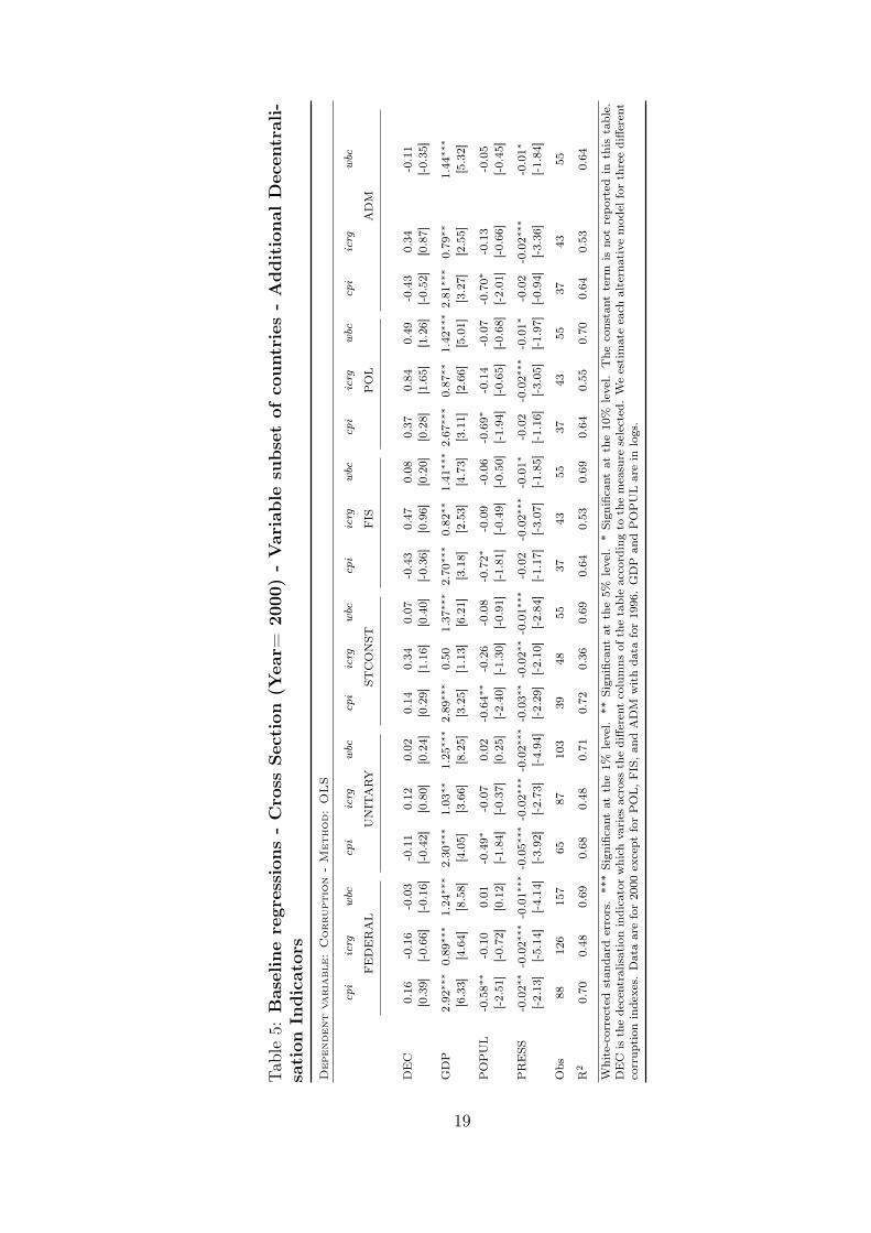
Table5:

Baselineregression

s-Cross

Section

(Year=

2000

)-Variable

subsetof

countries

-Additional

Decentrali-

sation

Indicators

Dep

enden

tva

ria

ble:

Corru

ptio

n-

Met

hod:

OLS

cpi

icrg

wbc

cpi

icrg

wbc

cpi

icrg

wbc

cpi

icrg

wbc

cpi

icrg

wbc

cpi

icrg

wbc

FEDERAL

UNITARY

STCONST

FIS

POL

ADM

DEC

0.16

-0.16

-0.03

-0.11

0.12

0.02

0.14

0.34

0.07

-0.43

0.47

0.08

0.37

0.84

0.49

-0.43

0.34

-0.11

[0.39]

[-0.66]

[-0.16]

[-0.42]

[0.80]

[0.24]

[0.29]

[1.16]

[0.40]

[-0.36]

[0.96]

[0.20]

[0.28]

[1.65]

[1.26]

[-0.52]

[0.87]

[-0.35]

GDP

2.92

∗∗∗

0.89

∗∗∗

1.24

∗∗∗

2.30

∗∗∗

1.03

∗∗1.25

∗∗∗

2.89

∗∗∗

0.50

1.37

∗∗∗

2.70

∗∗∗

0.82

∗∗1.41

∗∗∗2.67

∗∗∗

0.87

∗∗1.42

∗∗∗2.81

∗∗∗

0.79

∗∗1.44

∗∗∗

[6.33]

[4.64]

[8.58]

[4.05]

[3.66]

[8.25]

[3.25]

[1.13]

[6.21]

[3.18]

[2.53]

[4.73]

[3.11]

[2.66]

[5.01]

[3.27]

[2.55]

[5.32]

POPUL

-0.58∗

∗-0.10

0.01

-0.49∗

-0.07

0.02

-0.64∗

∗-0.26

-0.08

-0.72∗

-0.09

-0.06

-0.69∗

-0.14

-0.07

-0.70∗

-0.13

-0.05

[-2.51]

[-0.72]

[0.12]

[-1.84]

[-0.37]

[0.25]

[-2.40]

[-1.30]

[-0.91]

[-1.81]

[-0.49]

[-0.50]

[-1.94]

[-0.65]

[-0.68]

[-2.01]

[-0.66]

[-0.45]

PRESS

-0.02∗

∗-0.02∗

∗∗-0.01∗

∗∗-0.05∗

∗∗-0.02∗

∗∗-0.02∗

∗∗-0.03∗

∗-0.02∗

∗-0.01∗

∗∗-0.02

-0.02∗

∗∗-0.01∗

-0.02

-0.02∗

∗∗-0.01∗

-0.02

-0.02∗

∗∗-0.01∗

[-2.13]

[-5.14]

[-4.14

][-3.92]

[-2.73]

[-4.94]

[-2.29]

[-2.10]

[-2.84]

[-1.17]

[-3.07]

[-1.85]

[-1.16]

[-3.05]

[-1.97]

[-0.94]

[-3.36]

[-1.84]

Obs

88126

157

6587

103

3948

5537

4355

3743

5537

4355

R2

0.70

0.48

0.69

0.68

0.48

0.71

0.72

0.36

0.69

0.64

0.53

0.69

0.64

0.55

0.70

0.64

0.53

0.64

White-corrected

stan

dard

errors.***Sign

ificant

atthe1%

level.

**Sign

ificant

atthe5%

level.

*Sign

ificant

atthe10%

level.

The

constant

term

isno

trepo

rted

inthis

table.

DEC

isthedecentralisationindicatorwhich

varies

across

thediffe

rent

columns

ofthetableaccordingto

themeasure

selected.Weestimateeach

alternativemod

elforthreediffe

rent

corrup

tion

indexes.

Dataarefor20

00except

forPOL,FIS,an

dADM

withda

tafor19

96.GDP

andPOPULarein

logs.

19

of elected sub-national tiers (vertical decentralisation according to Treisman). In

no case is there any evidence of a relationship of any kind with corruption. This

is consistent with Treisman (2002a) who found that the number of sub-national

elected tiers is sensitive to the inclusion of a measure of GDP, one of the most

robust determinants of corruption, and country size. The existence of autonomous

contiguous regions may be in principle associated to lower corruption given that

these regions may be seen as checks on the central authority. But the fact that

most of these regions are associated to ethnic groups would probably act as a bal-

ancing act increasing corruption derived from ethnic or linguistic fragmentation.

The data suggest that auton and corruption are not directly related.

From our discussion above, it is clear that there are relatively few measures of

decentralisation that directly impact on corruption and even fewer that are robust

across the different indices of corruption typically used in the literature. Some

combinations of the significant variables uncovered are also somewhat puzzling.

For example, how is that federal countries are more corrupt than unitary countries

if market decentralisation is associated with lower corruption? Is the relationship

between market decentralisation and corruption the same at different levels of

market and political decentralisation? Why is political decentralisation not re-

lated to corruption in light of all the electoral accountability and local capture

theories? To what extent is spatial decentralisation associated to more efficient

organisation and delivery of public services? Does granting decision-making au-

thority to sub-national governments have different impact on corruption if electoral

decentralisation is in place?

4.2 Multi-dimensional corruption

One of our objectives in this work is to try to analyse a number of dimensions

of decentralisation and their relationship with corruption. As we noticed earlier,

the literature in this area is somewhat vague in describing the way in which dif-

ferent aspects of decentralisation may be simultaneously important. In Table 6

we concentrate on the main variables found to be significant in Table 4. Model 1

replicates the very basic model included in Table 4 with only the market decen-

tralisation indicator (rev) controlled for. In model 5 we include both the market

decentralisation and unitary history measures, in model 7 we add the political

20

decentralisation measure muni and in model 8 we add the spatial decentralisation

control, locj. Only the results for market and constitutional decentralisation are

robust; indeed their estimated effects increase in size and significance compared to

the earlier regressions. These results do not change when we include the spatial

and political decentralisation measures, excluding the market and constitutional

decentralisation measures. This regression also highlights a limitation of trying to

control for many dimensions of decentralisation, since the number of observations

drops markedly. The main drop in the number of observations from model 5 to 12

is caused by the inclusion of muni for which we have many missing observations.

We have also tested (although they are not shown in the table) the other indicators

for constitutional (federal), political (state, stconst) and spatial (tiers, regj ) de-

centralisation in the regressions as alternative indicators of unitaryhis, muni and

locj. In no case are the coefficients significantly different from zero.

As a final check on these models, we have included additional controls in the speci-

fication. The idea behind this is to account for the possibility that there are direct

and independent significant effects on corruption of variables not related to decen-

tralisation. In general, when papers examine the relationship between federalism

and corruption, they either exclude any other aspect of market decentralisation

from the specification [Treisman (2000)] or they fail to find any significant direct

effect of federalism on corruption [Fisman and Gatti (2002)]. Models 9 through

12 experiment using the specification given by model 7 (market, political and con-

stitutional decentralisation altogether) and adding other standard controls that

have been suggested as robust determinants of corruption elsewhere [Treisman

(2000), La Porta et al. (1999) and Serra (2006)]. The extent of political rights, the

ethno-linguistic fractionalization index, and dummies for British colonial history

and protestantism as dominant religion come out insignificant without introducing

any significant changes to the coefficients of our main variables of interest19.19We have also used alternative indicators for each of these controls and have also controlled

for other potential determinants of corruption with the results being largely unchanged. Someof the results are included in the Appendix and all of them may be obtained from the authors.

21

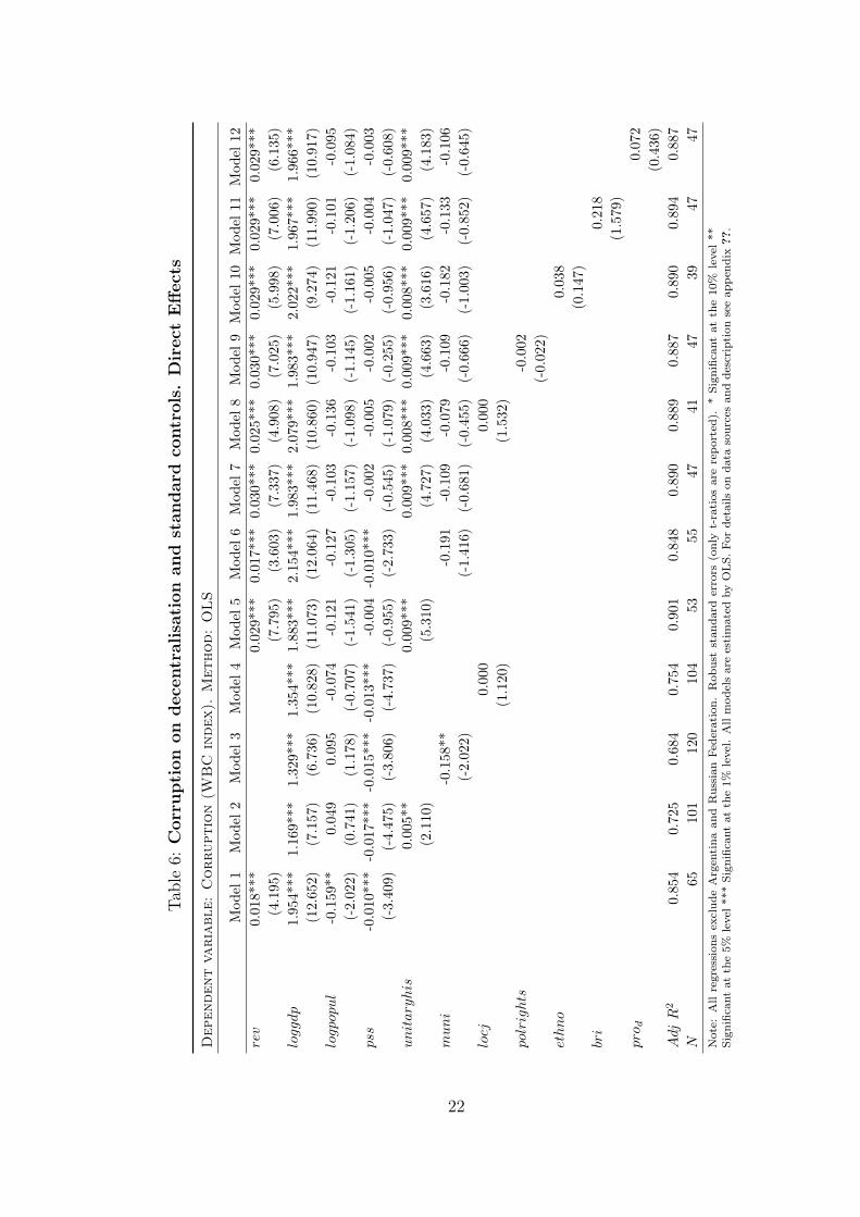
Table6:

Corruption

ondecentralisationan

dstan

dardcontrols.DirectEffects

Dep

enden

tva

ria

ble:

Corru

ptio

n(W

BC

index

).M

ethod:

OLS

Mod

el1

Mod

el2

Mod

el3

Mod

el4

Mod

el5

Mod

el6

Mod

el7

Mod

el8

Mod

el9

Mod

el10

Mod

el11

Mod

el12

rev

0.018***

0.029***

0.017***

0.030***

0.025***

0.030***

0.029***

0.029***

0.029***

(4.195)

(7.795)

(3.603)

(7.337)

(4.908)

(7.025)

(5.998)

(7.006)

(6.135)

loggdp

1.954***

1.169***

1.329***

1.354***

1.883***

2.154***

1.983***

2.079***

1.983***

2.022***

1.967***

1.966***

(12.652)

(7.157)

(6.736)

(10.828)

(11.073)

(12.064)

(11.468)

(10.860)

(10.947)

(9.274)

(11.990)

(10.917)

logpop

ul

-0.159**

0.049

0.095

-0.074

-0.121

-0.127

-0.103

-0.136

-0.103

-0.121

-0.101

-0.095

(-2.022)

(0.741)

(1.178)

(-0.707)

(-1.541)

(-1.305)

(-1.157)

(-1.098)

(-1.145)

(-1.161)

(-1.206)

(-1.084)

pss

-0.010***

-0.017***

-0.015***

-0.013***

-0.004

-0.010***

-0.002

-0.005

-0.002

-0.005

-0.004

-0.003

(-3.409)

(-4.475)

(-3.806)

(-4.737)

(-0.955)

(-2.733)

(-0.545)

(-1.079)

(-0.255)

(-0.956)

(-1.047)

(-0.608)

unit

ary

his

0.005**

0.009***

0.009***

0.008***

0.009***

0.008***

0.009***

0.009***

(2.110)

(5.310)

(4.727)

(4.033)

(4.663)

(3.616)

(4.657)

(4.183)

muni

-0.158**

-0.191

-0.109

-0.079

-0.109

-0.182

-0.133

-0.106

(-2.022)

(-1.416)

(-0.681)

(-0.455)

(-0.666)

(-1.003)

(-0.852)

(-0.645)

locj

0.000

0.000

(1.120)

(1.532)

pol

rights

-0.002

(-0.022)

ethno

0.038

(0.147)

bri

0.218

(1.579)

pro

d0.072

(0.436)

Adj

R2

0.854

0.725

0.684

0.754

0.901

0.848

0.890

0.889

0.887

0.890

0.894

0.887

N65

101

120

104

5355

4741

4739

4747

Note:

Allregression

sexclud

eArgentina

andRussian

Federation

.Rob

uststan

dard

errors

(onlyt-ratios

arerepo

rted).

*Sign

ificant

atthe10

%level**

Sign

ificant

atthe5%

level*

**Sign

ificant

atthe1%

level.Allmod

elsareestimated

byOLS.

Fordetails

onda

tasourcesan

ddescriptionseeap

pend

ix??

.

22

4.3 Interaction effects

Before we move on to consider the models with indirect and interaction effects we

think it may be useful to examine the relationship between corruption and a few

of the decentralisation indicators at different degrees of decentralisation. First,

we split the sample according to certain criterion and perform a rolling regres-

sion. This procedure takes several steps involving ranking the observations on the

variable of interest (market, political constitutional or spatial decentralisation in

our case) and then running an initial regression for the observations satisfying the

chosen criterion. For example, we may choose as our initial sub-sample the ob-

servations for which market decentralisation is less than the mean value. Another

alternative is to choose an arbitrary sub-sample size and define that as the initial

sub-sample. We then run a regression using this sub-sample, obtain the estimates

and statistics and record the values. Next we add the nearest highest-ranked ob-

servation not included in the initial sub-sample and we drop the lowest-ranked

observation included in the initial sub-sample. We always keep the sub-sample

size constant throughout this analysis, thus making sure any changes are not due

to the increase/decrease in sample size. We continue this procedure until the last

(highest-ranked) observation is added and we record the estimates.

The only limitation to this procedure is that we can only perform it for the con-

tinuous measures of decentralisation, since using a discrete or categorical measure

will result in all countries having the same rank within each category. There-

fore we perform this analysis for three continuous measures of decentralisation:

exp, rev, and unitaryhis. In the exp and rev cases we are left with 68 and 67

observations respectively and we choose a sub-sample size of 30 for each20. We

use the World Bank Control of Corruption index which has been chosen as our

main corruption index. We summarize the results of the analysis in the following

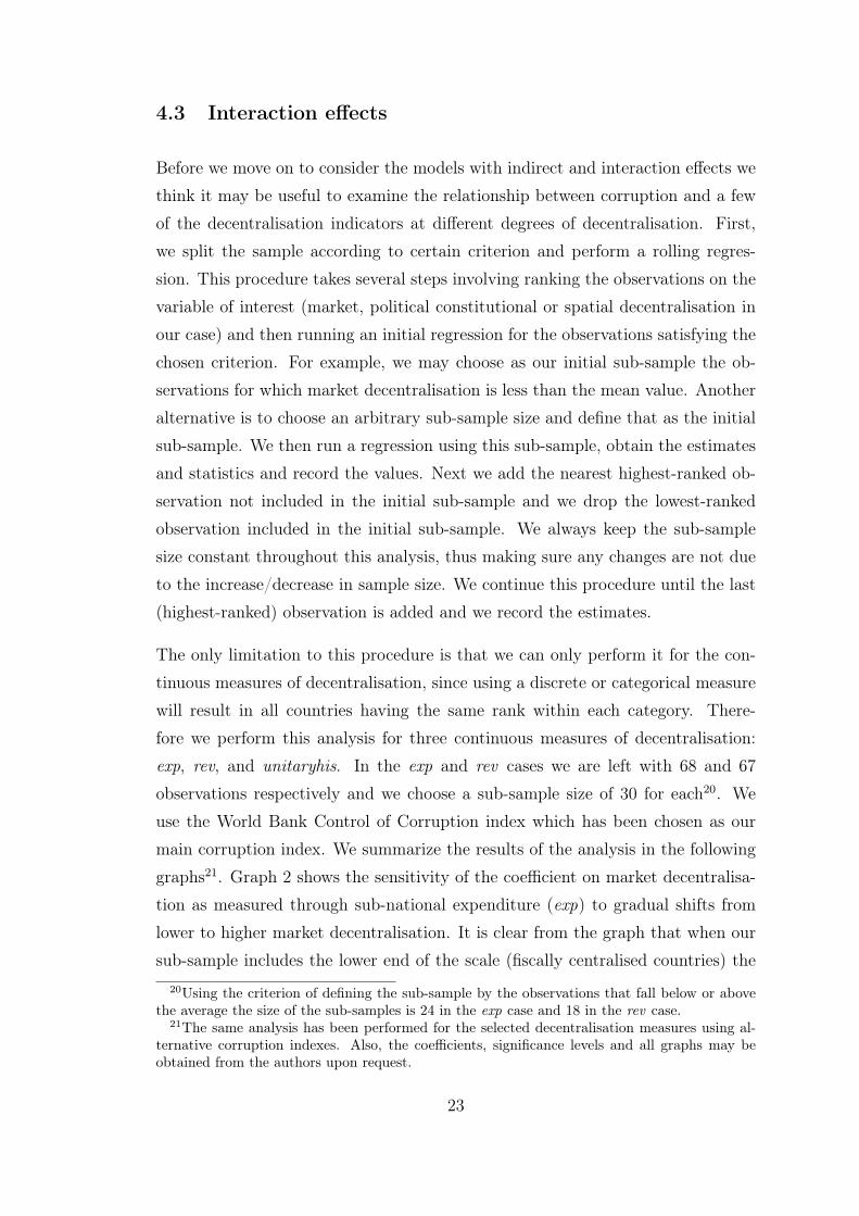
graphs21. Graph 2 shows the sensitivity of the coefficient on market decentralisa-

tion as measured through sub-national expenditure (exp) to gradual shifts from

lower to higher market decentralisation. It is clear from the graph that when our

sub-sample includes the lower end of the scale (fiscally centralised countries) the20Using the criterion of defining the sub-sample by the observations that fall below or above

the average the size of the sub-samples is 24 in the exp case and 18 in the rev case.21The same analysis has been performed for the selected decentralisation measures using al-

ternative corruption indexes. Also, the coefficients, significance levels and all graphs may beobtained from the authors upon request.

23

coefficient of market decentralisation on corruption is negative (the dots in the

figure) although almost never significant at the 10% level. But as we gradually

include more fiscally decentralised countries in our sub-sample, the coefficients

become positive and significant for a high percentage of regressions. The fact that

the graph depicts a smooth transition from negative to positive coefficients when

market decentralisation increases is indicative of the presence of heterogeneity in

the relationship between these two variables22.

Figure 2: Rolling regression for exp and wbc

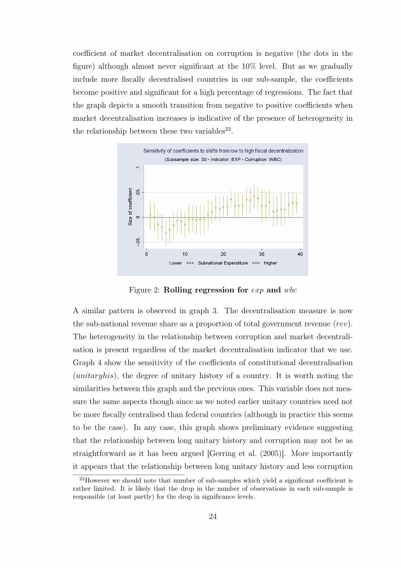
A similar pattern is observed in graph 3. The decentralisation measure is now

the sub-national revenue share as a proportion of total government revenue (rev).

The heterogeneity in the relationship between corruption and market decentrali-

sation is present regardless of the market decentralisation indicator that we use.

Graph 4 show the sensitivity of the coefficients of constitutional decentralisation

(unitaryhis), the degree of unitary history of a country. It is worth noting the

similarities between this graph and the previous ones. This variable does not mea-

sure the same aspects though since as we noted earlier unitary countries need not

be more fiscally centralised than federal countries (although in practice this seems

to be the case). In any case, this graph shows preliminary evidence suggesting

that the relationship between long unitary history and corruption may not be as

straightforward as it has been argued [Gerring et al. (2005)]. More importantly

it appears that the relationship between long unitary history and less corruption22However we should note that number of sub-samples which yield a significant coefficient is

rather limited. It is likely that the drop in the number of observations in each sub-sample isresponsible (at least partly) for the drop in significance levels.

24

is being driven by the sub-sample of historically unitarist countries which have a

higher GDP per capita than the rest of the countries. In fact, the average GDP

per capita for the sub-sample of historically unitarist countries is almost three

times that of the historically federal countries23.

Figure 3: Rolling regression for rev and wbc

From the previous analysis it is evident that aspects of market and constitutional

decentralisation are associated with corruption. It also appears that there may

be some heterogeneity in the relationship between these variables and corruption.

The results yielded by the rolling regression analysis suggest this may the case.

Furthermore, we would like to examine the form of heterogeneity existent in this

relationship and in order to do this we proceed with additional econometric anal-

ysis, this time adding interaction terms to the baseline specifications.

Now we want to examine the possibility that other aspects of decentralisation may

affect corruption indirectly or that market and constitutional decentralisation may

have an indirect rather than a direct effect on corruption. We use a base specifica-

tion including both controls for market and constitutional decentralisation and we

introduce some interactions terms. In principle, we would expect that other as-

pects of decentralisation or of the institutional environment may affect the impact

of market or constitutional decentralisation on corruption. The interactions that

we propose in this section are based in theoretical presumptions provided by the

relevant literature. For instance, we interact the market decentralisation control23We split the sample into two grouping the countries above and below the average of unitary

history.

25

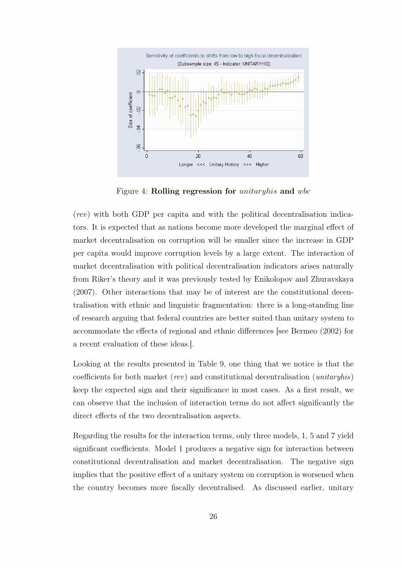
Figure 4: Rolling regression for unitaryhis and wbc

(rev) with both GDP per capita and with the political decentralisation indica-

tors. It is expected that as nations become more developed the marginal effect of

market decentralisation on corruption will be smaller since the increase in GDP

per capita would improve corruption levels by a large extent. The interaction of

market decentralisation with political decentralisation indicators arises naturally

from Riker’s theory and it was previously tested by Enikolopov and Zhuravskaya

(2007). Other interactions that may be of interest are the constitutional decen-

tralisation with ethnic and linguistic fragmentation: there is a long-standing line

of research arguing that federal countries are better suited than unitary system to

accommodate the effects of regional and ethnic differences [see Bermeo (2002) for

a recent evaluation of these ideas.].

Looking at the results presented in Table 9, one thing that we notice is that the

coefficients for both market (rev) and constitutional decentralisation (unitaryhis)

keep the expected sign and their significance in most cases. As a first result, we

can observe that the inclusion of interaction terms do not affect significantly the

direct effects of the two decentralisation aspects.

Regarding the results for the interaction terms, only three models, 1, 5 and 7 yield

significant coefficients. Model 1 produces a negative sign for interaction between

constitutional decentralisation and market decentralisation. The negative sign

implies that the positive effect of a unitary system on corruption is worsened when

the country becomes more fiscally decentralised. As discussed earlier, unitary

26

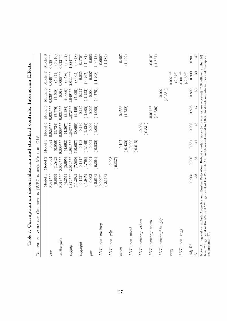
Table7:

Corruption

ondecentralisationan

dstan

dardcontrols.InteractionEffects

Dep

enden

tva

ria

ble:

Corru

ptio

n(W

BC

index

).M

ethod:

OLS

Mod

el1

Mod

el2

Mod

el3

Mod

el4

Mod

el5

Mod

el6

Mod

el7

Mod

el8

rev

0.037***

0.064

0.031

0.028***

0.031***

0.030***

0.040***

0.038***

(6.866)

(1.542)

(0.856)

(5.724)

(7.776)

(7.508)

(5.341)

(6.216)

unit

ary

his

0.013***

0.009***

0.009***

0.009***

0.031***

0.018

0.008***

0.032***

(4.251)

(5.095)

(4.692)

(4.367)

(3.184)

(0.666)

(3.586)

(3.262)

loggdp

1.876***

2.064***

1.984***

1.847***

1.872***

1.949***

2.011***

1.884***

(11.292)

(7.580)

(10.607)

(8.698)

(9.459)

(7.339)

(8.005)

(9.848)

logpop

ul

-0.152*

-0.131*

-0.103

-0.136

-0.135

-0.117

-0.035

-0.170*

(-1.945)

(-1.768)

(-1.146)

(-1.424)

(-1.605)

(-1.452)

(-0.267)

(-1.981)

pss

-0.003

-0.004

-0.002

-0.006

-0.005

-0.004

-0.007

-0.003

(-0.613)

(-0.864)

(-0.530)

(-1.051)

(-1.005)

(-0.779)

(-1.208)

(-0.613)

IN

T:r

ev·u

nit

ary

-0.000**

-0.000*

(-2.113)

(-1.789)

IN

T:r

ev·g

dp

-0.008

(-0.837)

muni

-0.107

0.456*

0.407

(-0.430)

(1.732)

(1.499)

IN

T:r

ev·m

uni

-0.000

(-0.015)

IN

T:u

nit

ary·e

thno

-0.004

(-0.831)

IN

T:u

nit

ary·m

uni

-0.011**

-0.010*

(-2.236)

(-1.857)

IN

T:u

nit

ary

his·g

dp

-0.002

(-0.331)

regj

0.007**

(2.372)

IN

T:r

ev·r

egj

-0.001**

(-2.582)

Adj

R2

0.905

0.900

0.887

0.903

0.898

0.899

0.900

0.901

N53

5347

4547

5330

47Note:

Allregression

sexclud

eArgentina

andRussian

Federation

.Rob

uststan

dard

errors

(onlyt-ratios

arerepo

rted).

*Sign

ificant

atthe10%

level*

*Sign

ificant

atthe5%

level*

**Sign

ificant

atthe1%

level.Allmod

elsareestimated

byOLS.

Fordetails

onda

tasourcesan

ddescription

seeap

pend

ix??

.

27

systems need not be incompatible with other aspects of decentralisation. The sign

of this interaction is somewhat surprising. One possible reason for this to happen

is that when countries become more fiscally decentralized the effectiveness of a

unitary structure to control and monitor the growing amount of resources allocated

to the decentralised units decreases. In any event, even when the coefficient is

negative and significant, its size is very small.

Model 5 yields a negative sign for the interaction term between political and

constitutional decentralisation. Again, this means that the positive effect of con-

stitutional decentralisation on corruption worsens when the country becomes more

politically decentralised. Finally, the results for model 7 imply that the positive

effect of market decentralisation on corruption is worsened when the number of

intermediate jurisdictions grows. We have also tried other indicators of political

decentralisation interacted with market and constitutional decentralisation mea-

sures but none of these other interaction terms was found significantly different

from zero.

In model 8 we include both direct effects of fiscal and constitutional decentralisa-

tion and the interaction terms from models 1 and 5. The rationale for this is to

test whether these interactions still hold when included within the same econo-

metric model. Model 8 is clear in that it renders both direct effects and both

interaction terms significant. The signs are the same as those obtained in the

previous models. In this way, Model 8 stands both as a robustness check on the

model with direct effects and also as a more comprehensive model for describing

the empirical relationship between corruption and decentralisation. As it is clear

from this model, our suggestions earlier in this research have been upheld by the

analysis of the data.

5 Conclusions

The last 30 years have seen a large number of countries embark in some form

of decentralisation. While the causes of this trend are in general precise and

well-known, its consequences are much less certain and by no means definitive.

Evaluating the results of decentralisation is not an easy task. Case studies provide

28

an important source of evidence but generalisation is not straightforward. Cross-

country and panel-data studies are becoming more common but suffer from two

main problems. On one hand, there are data issues. On the other hand, there

are modelling problems. These two elements act as limiting forces on both the

quantity and quality of empirical research. Nevertheless, there seems to be a

renewed scholarly commitment to take the empirics to new levels.

We need better and more thorough empirical studies. We argue that a first step

towards this is to understand decentralisation as multidimensional phenomenon

that has a large variety of effects. In this sense, we should ideally aim at identify-

ing these dimensions and postulating the likely effects and the interrelationships

between them. In this sense, the theoretical literature has provided with interest-

ing insights that have been often left unexplored by the empirical literature until

very recently. Our work in this paper has shown why this approach is important,

what are the some of questions still unresolved in the empirical literature and how

to attempt a sensible approach to tackling these issues.

Recent literature has acknowledged the presence of a number of aspects that make

the study of the relationship between decentralisation and corruption less obvious.

First, it has been recognized that different dimensions of decentralisation exist

and that they have complex interrelations. Second, it has been argued that the

extent and effects of decentralisation may depend on the existence and extent

of other dimensions of decentralisation. Although these ideas are not new, they

are becoming increasingly common in the empirical literature. Finally, it has

also been suggested that different dimensions of decentralisation may co-evolve

and their interactions over time might have a strong effect on corruption and the

institutional quality.

Our results in this paper may provide a few insights regarding the policy debate

on the effects of decentralisation. In particular, as we have seen, the positive effect

of market decentralisation on corruption seems to be larger when countries have

a deeply rooted unitarist history. While this result seems to be not so intuitive,

it is plausible that deepening fiscal decentralisation without changing the con-

stitutional basis or government organisation may indeed be associated to higher

corruption. After all, delegating more money to local governments which may

lack the autonomy to create taxes -as might the case in a strong unitary system-,

29

may encourage bad governance and corruption. Furthermore, a growing num-

ber of unitary countries are resorting to local democratization processes via local

elections or referenda voting. Our results suggest that a move to higher political

decentralisation may have associated higher corruption particularly if the country

is has a unitarist tradition and low levels of market decentralisation. It should be

noted, that according to our results, the existence of long-standing unitary system

has both direct and indirect association with corruption. As these have opposite

signs, the overall result is uncertain and essentially an empirical matter.

Finally, although we have shown that our results are consistent with a sensible

specification, and robust to controlling for different variables and data, we are

rather shy regarding the direction of the causation. The aim in this paper has

been to analyse the effect that the several interrelationships between multiple

dimensions of decentralisation have on corruption. There may be additional con-

siderations if endogeneity of the regressors is a possibility. In conclusion, the issue

of whether decentralisation leads to more or less corruption is still uncertain and

much more empirical research is needed. But we believe that this future empir-

ical research should be aimed at exploring the interrelations of different aspects

or dimensions of decentralisation. The study of these aspects has been suggested

and carried out by Barenstein and de Mello (2001), Rodden (2002), Treisman

(2002b,a) and Enikolopov and Zhuravskaya (2007). Our study contributes to this

literature by both reinforcing some of the earlier findings and obtaining some new

evidence.

References

Ames, B. (1994). The reverse coattails effect: Local party organization in the 1989

brazilian presidential election. American Political Science Review.

Aranson, P. H. (1990). Federalism: The reasons for rules. Cato Journal, 10(1):17–

38.

Bardhan, P. and Mookherjee, D. (2000). Capture and governance at local and

national levels. American Economic Review, 90(2):135–139.

Barenstein, M. and de Mello, L. (2001). Fiscal decentralization and governance:

30

A cross-country analysis. IMF Working Papers 01/71, International Monetary

Fund.

Bermeo, N. (2002). A new look at federalism: The import of institutions. Journal

of Democracy, 13(2):96–110.

Brunetti, A. and Weder, B. (2003). A free press is bad news for corruption. Journal

of Public Economics, 87:1801–1824.

Chowdhury, S. K. (2004). The effect of democracy and press freedom on corrup-

tion: an empirical test. Economics Letters, 85(1):93–101.

Ebel, R. D. and Yilmaz, S. (2002). On the measurement and impact of fiscal

decentralization. Policy Research Working Paper Series 2809, The World Bank.

Elazar, D. (1995). From statism to federalism: A paradigm shift. Publius, 25(2):5–

18.

Enikolopov, R. and Zhuravskaya, E. (2007). Decentralization and political insti-

tutions. Journal of Public Economics.

Fisman, R. and Gatti, R. (2002). Decentralization and corruption: evidence across

countries. Journal of Public Economics, 83:325–345.

Fjelstad, O.-H. (2004). Decentralisation and corruption: A review. CMI Working

Paper 10, Bergen: Chr. Michelsen Institute.

Freille, S., Haque, E., and Kneller, R. (forthcoming). A contribution to the em-

pirics of press freedom and corruption. European Journal of Political Economy.

Gelineau, F. and Remmer, K. L. (2006). Political decentralization and electoral

accountability: The argentine experience, 1983-2001. British Journal of Political

Science.

Gerring, J., Moreno, C., and Thacker, S. C. (2005a). Are unitary systems better

than federal systems? Unpublished manuscript.

Gerring, J., Moreno, C., and Thacker, S. C. (2005b). Centripetal democratic

governance: A theory and global inquiry. American Political Science Review,

99(4):567–581.

31

Goldsmith, A. A. (1999). Slapping the grasping hand: Correlates of political

corruptionin emerging markets. American Journal of Economics and Sociology,

58(3):866–883.

Huther, J. and Shah, A. (1998). Applying a simple measure of good governance

to the debate on fiscal decentralization. Policy Research Working Paper Series

1894, The World Bank.

Kuncoro, A. (2004). Bribery in indonesia: Some evidence from micro-level data.

Bulletin of Indonesian Economic Studies, 40(3):329–354.

La Porta, R., Lopez-de Silanes, F., Shleifer, A., and Vishny, R. (1999). The quality

of government. Journal of Law, Economics and Organization, 15(1):222–79.

Oates, W. (2005). Toward a second-generation theory of fiscal federalism. Inter-

national Tax and Public Finance, 12(4):349–373.

Oates, W. E. (1972). Fiscal federalism. New York: Harcourt Brace Jovanovich.

Persson, T., Tabellini, G., and Trebbi, F. (2003). Electoral rules and corruption.

Journal of the European Economic Association, 1(4):958–989.

Riker, W. (1964). Federalism: Origins, operation, significance. Little, Brown and

Co., Boston, MA.

Rodden, J. (2002). The dilemma of fiscal federalism: Grants and fiscal performance

around the world. American Journal of Political Science, 46(3):670–687.

Rondinelli, D. A. (2006). International Development Governance, chapter Decen-

tralization and development. CRC Press.

Samuels, D. (2000). The gubernatorial coattails effect: Federalism and congres-

sional elections in brazil. Journal of Politics.

Schneider, A. (2003). Decentralization: Conceptualization and measurement.

Studies in Comparative International Development, 38(3):32–56.

Serra, D. (2006). Empirical determinants of corruption: A sensitivity analysis.

Public Choice, 126(1):225–256.

Tiebout, C. (1956). A pure theory of local expenditures. Journal of Political

Economy, 64(5):416–424.

32

Treisman, D. (2000). The causes of corruption: A cross-national study. Journal

of Public Economics, 76(3):399–457.

Treisman, D. (2002a). Decentralization and the quality of government. Unpub-

lished manuscript.

Treisman, D. (2002b). Defining and measuring decentralization: A global perspec-

tive. Unpublished manuscript.

Wade, R. (1997). How infrastructure agencies motivate staff: Canal irrigation in

india and the republic of korea. In Mody, A., editor, Infrastructure Strategies

in East Asia. World Bank.

Wu, X. (2005). Corporate governance and corruption. Governance: An Interna-

tional Journal of Policy, 18(2):151–170.

33

6 Appendix

34

Table8:

Pairw

isecorrelationsam

ongselected

decentralisationindicators

exp

rev

muni

sta

const

auth

auto

dec

4dec

2fed

1fed

2fed

iunit

uhis

fis

pol

adm

tier

regj

locj

exp

1.00

rev

0.95

1.00

muni

0.06

0.08

1.00

sta

0.41

0.38

0.55

1.00

const

0.52

0.47

0.31

0.29

1.00

auth

0.55

0.57

0.52

0.69

0.31

1.00

auto

0.24

0.24

0.12

0.08

0.28

0.19

1.00

dec

40.53

0.48

0.89

0.89

0.26

0.71

0.26

1.00

dec

20.56

0.52

0.88

0.88

0.29

0.71

0.39

0.99

1.00

fed

10.47

0.44

0.21

0.36

0.48

0.67

0.07

0.31

0.32

1.00

fed

20.45

0.39

0.18

0.34

0.45

0.63

0.24

0.41

0.43

0.62

1.00

fed

i-0.47

-0.47

-0.25

-0.32

-0.48

-0.61

0.00

-0.35

-0.35

-0.78

-0.62

1.00

unit

-0.63

-0.65

-0.15

-0.41

-0.48

-0.61

-0.09

-0.30

-0.33

-0.88

-0.69

0.86

1.00

uhis

-0.24

-0.32

0.14

0.04

-0.32

-0.19

-0.10

0.18

0.17

-0.33

-0.20

0.31

0.38

1.00

fis

0.51

0.54

0.13

-0.01

0.08

0.39

0.04

0.22

0.20

0.17

0.03

-0.01

0.21

0.16

1.00

pol

-0.03

0.15

-0.11

0.06

0.25

-0.23

0.03

-0.01

-0.01

-0.01

0.05

-0.13

-0.17

0.06

-0.04

1.00

adm

-0.04

-0.06

0.13

-0.15

0.01

0.24

0.02

0.53

0.55

0.03

-0.04

0.17

0.42

0.36

0.04

0.04

1.00

tier

0.22

0.13

0.48

0.36

0.50

0.40

0.05

0.42

0.42

0.44

0.35

-0.43

-0.42

0.14

-0.05

-0.16

-0.13

1.00

regj

-0.05

-0.04

0.12

0.00

-0.14

-0.04

-0.04

0.04

0.03

-0.14

-0.01

0.00

0.06

0.08

0.45

-0.09

0.25

0.01

1.00

locj

0.30

0.25

0.11

0.07

0.20

0.23

-0.03

0.22

0.23

0.27

0.20

-0.30

-0.28

-0.14

-0.10

-0.21

-0.12

0.19

0.00

1.00

Pairw

isecorrelations

arecalculated

foryear

2000.*Denotes

sign

ificanceat

the5%

level.

35

Table9:

Baselineregression

s-Cross

Section

(Year=

2000

)-Com

mon

subsetof

countries

Dep

enden

tva

ria

ble:

Corru

ptio

n-

Met

hod:

OLS

cpi

icrg

wbc

cpi

icrg

wbc

cpi

icrg

wbc

cpi

icrg

wbc

cpi

icrg

wbc

cpi

icrg

wbc

EXP

REV

MUNI

STATE

AUTHOR

AUTON

DEC

0.03

∗∗0.02

∗∗0.01

0.03

∗∗0.02

∗0.01

∗∗-0.74∗

∗∗-0.16

-0.35∗

∗∗-0.15

-0.25∗

∗-0.04

-0.40

-0.64∗

∗∗-0.30

-0.44

-0.28

-0.07

[2.31]

[2.35]

[1.47]

[2.05]

[1.76]

[1.22]

[-3.01]

[-1.4]

[-3.17]

[-0.69]

[-1.95]

[-0.46]

[-0.71]

[-2.58]

[-1.21]

[-0.91]

[-1.21

][-0.28]

GDP

3.75

∗∗∗

0.83

∗1.83

∗∗∗

3.93

∗∗∗

0.87

∗1.90

∗∗∗

3.85

∗∗∗

1.23

∗∗∗

1.86

∗∗∗

3.40

∗∗∗

1.23

∗∗∗

1.64

∗∗∗

3.50

∗∗∗

1.24

∗∗1.70

∗∗∗

2.89

∗∗∗

0.97

∗∗∗

1.45

∗∗∗

[6.48]

[1.92]

[7.4]

[6.58]

[1.92]

[7.55]

[8.22]

[4.86]

[8.33]

[6.64]

[5.8]

[6.78]

[4.7]

[3.97]

[4.69]

[6.16]

[4.78]

[6.5]

POPUL

-0.59∗

∗-0.54∗

∗∗-0.18∗

-0.47∗

∗-0.52∗

∗∗-0.13

-0.39∗

-0.43∗

∗∗-0.13

-0.52∗∗

-0.35∗∗

-0.19∗

-0.30

-0.27

-0.05

-0.63∗∗

∗-0.50∗∗

∗-0.24∗∗

[-2.67]

[-3.53]

[-1.82]

[-2.15]

[-3.42]

[-1.37]

[-1.82]

[-2.95]

[-1.3]

[-2.46]

[-2.33]

[-1.9]

[-0.97]

[-1.20

][-0.34]

[-3.15]

[-3.86]

[-2.6]

PRESS

-0.02∗

-0.03∗

∗∗-0.02∗

∗∗-0.02∗

∗-0.03∗

∗∗-0.02∗

∗∗-0.02∗

∗-0.02∗

∗∗-0.01∗

∗∗-0.02∗

-0.02∗

∗∗-0.01∗

∗-0.02

-0.02∗

∗∗-0.02∗

∗∗-0.02∗

∗-0.02∗

∗∗-0.01∗

∗

[-2.39]

[-3.42]

[-3.25]

[-2.35]

[-3.41]

[-3.23]

[-2.51]

[-4.8]

[-3.03]

[-1.9]

[-5.18]

[-2.32]

[-1.17]

[-3.82

][-1.61]

[-2.18]

[-5.00]

[-2.42]

Obs

5555

5554

5454

7171

7176

7676

3737

3779

7979

R2

0.77

0.63

0.83

0.76

0.63

0.83

0.74

0.64

0.8

0.71

0.65

0.78

0.69

0.68

0.72

0.71

0.66

0.76

cpi

icrg

wbc

cpi

icrg

wbc

cpi

icrg

wbc

cpi

icrg

wbc

cpi

icrg

wbc

cpi

icrg

wbc

DECENT4

FEDIN

DEX

UNITARYHIS

TIE

RS

REGJ

LOCJ

DEC

-0.30∗

-0.19∗

∗-0.14∗

∗0.04

0.06

0.04

0.01

∗∗0.00

0.00

∗∗-0.11

-0.29∗

∗-0.03

0.00

0.00

0.00

0.00

0.00

∗∗0.00

[-1.9]

[-2.58]

[-2.05]

[0.37]

[0.92]

[0.80]

[2.17]

[0.41]

[2.12

[-0.56]

[-2.50]

[-0.29]

[0.45]

[-0.19]

[-0.15]

[0.88]

[2.64]

[1.75]

GDP

3.83

∗∗∗

1.35

∗∗∗

1.89

∗∗∗

2.86

∗∗∗

0.98

∗∗∗

1.45

∗∗∗

1.95

∗∗∗

0.60

∗0.97

∗∗∗

2.61

∗∗∗

1.00

∗∗∗

1.31

∗∗∗

2.61

∗∗∗

0.99

∗∗∗

1.23

∗∗∗

2.76

∗∗∗

1.04

∗∗∗

1.37

∗∗∗

[7.5]

[5.84]

[7.43]

[6.05]

[4.65]

[6.44]

[3.17]

[1.98]

[3.46]

[6.54]

[4.89]

[6.93]

[5.66]

[3.6]

[5.4]

[7.09]

[4.53]

[7.41]

POPUL

-0.36

-0.37∗

∗-0.10

-0.59∗

∗-0.40∗

∗-0.16

-0.35∗

-0.41∗

∗-0.13

-0.39∗

-0.33∗

∗-0.11

-0.42

-0.30

-0.06

-0.54∗

-0.55∗

∗-0.19

[-1.61]

[-2.28]

[-1.02]

[-2.08]

[-2.35]

[-1.33]

[-1.72]

[-2.52]

[-1.42]

[-1.72]

[-2.01]

[-1.07]

[-1.26

][-1.24]

[-0.47]

[-1.88]

[-2.92]

[-1.6]

PRESS

-0.02∗

∗-0.02∗

∗∗-0.01∗

∗∗-0.03∗

∗-0.02∗

∗∗-0.01∗

∗∗-0.05∗

∗∗-0.04∗

∗∗-0.03∗

∗∗-0.03∗

∗∗-0.03∗

∗∗-0.02∗

∗∗-0.05∗

∗∗-0.03∗

∗∗-0.03∗

∗∗-0.03∗

∗∗-0.02∗

∗∗-0.02∗

∗∗

[-2.05]

[-4.97]

[-2.59]

[-2.33]

[-4.68]

[-2.74]

[-3.33]

[-4.36]

[-4.21]

[-3.52]

[-5.35]

[-3.99]

[-3.8]

[-4.03]

[-4.4]

[-3.29]

[-4.1]

[-3.88]

Obs

6666

6682

8282

6464

6482

8282

5050

5076

7676

R2

0.71

0.65

0.78

0.69

0.64

0.76

0.71

0.60

0.78

0.69

0.66

0.77

0.74

0.59

0.78

0.69

0.62

0.77

White-corrected

stan

dard

errors.***Sign

ificant

atthe1%

level.

**Sign

ificant

atthe5%

level.

*Sign

ificant

atthe10%

level.

The

constant

term

isno

trepo

rted

inthis

table.

DEC

isthedecentralisationindicatorwhich

varies

across

thediffe

rent

columns

ofthetableaccordingto

themeasure

selected.Weestimateeach

alternativemod

elforthreediffe

rent

corrup

tion

indexes.

Dataarefor20

00except

forTIE

RS,

REGJan

dLOCJwithda

tafor1999.GDP

andPOPULarein

logs.

36

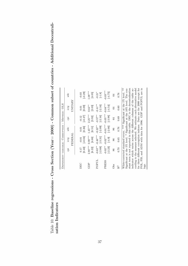
Table10

:Baselineregression

s-Cross

Section

(Year=

2000

)-Com

mon

subsetof

countries

-Additional

Decentrali-

sation

Indicators

Dep

enden

tva

ria

ble:

Corru

ptio

n-

Met

hod:

OLS

cpi

icrg

wbc

cpi

icrg

wbc

FEDERAL

UNITARY

DEC

0.17

-0.01

0.01

-0.12

0.01

-0.03

[0.40]

[-0.04]

[0.26]

[-0.47]

[0.09]

[-0.29]

GDP

2.88

∗∗∗

0.98

∗∗∗

1.45

∗∗∗

2.25

∗∗∗

0.64

∗∗1.08

∗∗∗

[6.22]

[4.68]

[6.51]

[3.92]

[2.03]

[4.05]

POPUL

-0.63∗

∗-0.46∗

∗∗-0.22∗

∗-0.57∗

∗-0.41∗

∗-0.21∗

[-2.68]

[-3.31]

[-2.09

][-2.16]

[-2.16]

[-1.8]

PRESS

-0.02∗

∗-0.02∗

∗∗-0.01∗

∗∗-0.05∗

∗∗-0.04∗

∗∗-0.03∗

∗∗

[-2.23]

[-4.9]

[-2.66]

[-3.98]

[-4.54]

[-4.75]

Obs

8686

8664

6464

R2

0.70

0.65

0.76

0.69

0.60

0.76

White-corrected

stan

dard

errors.**

*Sign

ificant

atthe1%

level.

**Sign

ificant

atthe5%

level.

*Sign

ificant

atthe10%

level.

The

con-

stan

tterm

isno

trepo

rted

inthis

table.

DEC

isthedecentralisation

indicatorwhich

varies

across

thediffe

rent

columns

ofthetableac-

cordingto

themeasure

selected.Weestimateeach

alternativemod

elforthreediffe

rent

corrup

tion

indexes.

Dataarefor2000

except

for

POL,FIS,an

dADM

withda

tafor1996.GDP

andPOPUL

arein

logs.

37

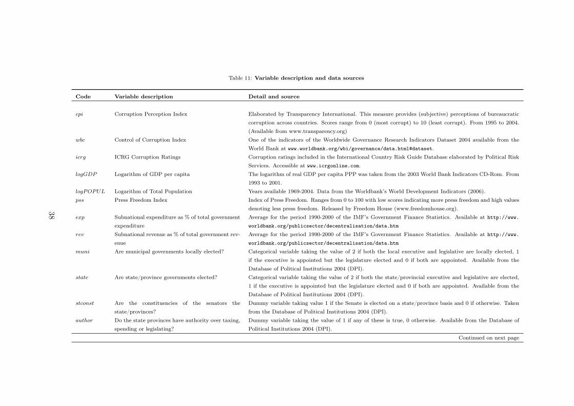
Table 11: Variable description and data sources

Code Variable description Detail and source

cpi Corruption Perception Index Elaborated by Transparency International. This measure provides (subjective) perceptions of bureaucratic

corruption across countries. Scores range from 0 (most corrupt) to 10 (least corrupt). From 1995 to 2004.

(Available from www.transparency.org)

wbc Control of Corruption Index One of the indicators of the Worldwide Governance Research Indicators Dataset 2004 available from the

World Bank at www.worldbank.org/wbi/governance/data.html#dataset.

icrg ICRG Corruption Ratings Corruption ratings included in the International Country Risk Guide Database elaborated by Political Risk

Services. Accessible at www.icrgonline.com.

logGDP Logarithm of GDP per capita The logarithm of real GDP per capita PPP was taken from the 2003 World Bank Indicators CD-Rom. From

1993 to 2001.

logPOPUL Logarithm of Total Population Years available 1969-2004. Data from the Worldbank’s World Development Indicators (2006).

pss Press Freedom Index Index of Press Freedom. Ranges from 0 to 100 with low scores indicating more press freedom and high values

denoting less press freedom. Released by Freedom House (www.freedomhouse.org).

exp Subnational expenditure as % of total government

expenditure

Average for the period 1990-2000 of the IMF’s Government Finance Statistics. Available at http://www.

worldbank.org/publicsector/decentralisation/data.htm

rev Subnational revenue as % of total government rev-

enue

Average for the period 1990-2000 of the IMF’s Government Finance Statistics. Available at http://www.

worldbank.org/publicsector/decentralisation/data.htm

muni Are municipal governments locally elected? Categorical variable taking the value of 2 if both the local executive and legislative are locally elected, 1

if the executive is appointed but the legislature elected and 0 if both are appointed. Available from the

Database of Political Institutions 2004 (DPI).

state Are state/province governments elected? Categorical variable taking the value of 2 if both the state/provincial executive and legislative are elected,

1 if the executive is appointed but the legislature elected and 0 if both are appointed. Available from the

Database of Political Institutions 2004 (DPI).

stconst Are the constituencies of the senators the

state/provinces?

Dummy variable taking value 1 if the Senate is elected on a state/province basis and 0 if otherwise. Taken

from the Database of Political Institutions 2004 (DPI).

author Do the state provinces have authority over taxing,

spending or legislating?

Dummy variable taking the value of 1 if any of these is true, 0 otherwise. Available from the Database of

Political Institutions 2004 (DPI).

Continued on next page

38

Table 11: (continued)

11 – Continued from previous page

Code Variable description Detail and source

auton Are there autonomous regions? Dummy variable taking the value of 1 if there exists autonomous contiguous regions, 0 otherwise. Available

from the Database of Political Institutions (DPI).

pol Factor score for political decentralization It ranges from 0 (low decentralization) to 1 (high decentralization). Source: ?. Year of observations, 1996.fis Factor score for fiscal decentralization It ranges from 0 (low decentralization) to 1 (high decentralization). Source: ?. Year of observations, 1996.adm Factor score for administrative decentralization It ranges from 0 (low decentralization) to 1 (high decentralization). Source: ?. Year of observations, 1996.dec2 Political decentralization index Constructed on the basis of aggregating auton, muni and state, from the Database of Political Institutions

(DPI).

dec4 Political decentralization index Constructed on the basis of aggregating muni and state, from the Database of Political Institutions (DPI).

federal Dummy for a federal country Variable taking the value of 1 if the country is federal, 0 otherwise. Based on the classification of Elazar (1995)

and the Handbook of Federal Countries. Other sources: CIA World Factbook, and selected Constitutions

of countries.

federal(2) Dummy for a federal country (broader concept) Variable taking the value of 1 if the country is federal, 0 otherwise. Based on the classification of Elazar (1995)

and the Handbook of Federal Countries. Other sources: CIA World Factbook, and selected Constitutions

of countries.

federal_alt Dummy for a federal country (Treisman) Dummy for federalism. Source: Treisman (2000).

fedindex Index of federalism Ranges from 1 to 5, with lower values indicating a more federal country. Source: STM103 Global Indicators

Shared Dataset V2.0 available at www.pippanorris.com.

unitary Index of unitarism Index taking the value of 0=federal (elective regional legislatures plus constitutional recognition of subna-

tional authority) 1= semi-federal (where there are elective legislatures at the regional level enjoying impor-

tant policy-making power but in which constitutional sovereignty is reserved to the national government)

2= unitary. Source: Gerring et al. (2005); ? available at www.pippanorris.com. Year=2000.

unitaryhis Index of Unitary History Cumulative index constructed on the basis of the annual values of unitary. Source: Gerring et al. (2005); ?available at www.pippanorris.com. Year=2000.

tiers Number of elected sub-national tiers Data for year 1999. Source: www.worldbank.org.

regj Number of intermediate jurisdictions Data for year 1999. Source: www.worldbank.org.

locj Number of local jurisdictions Data for year 1999. Source: www.worldbank.org.

polrights Index of political rights Political Rights Index (Freedom House). From 1 (most free) to 7 (least free). Source: www.freedomhouse.org.

Continued on next page

39

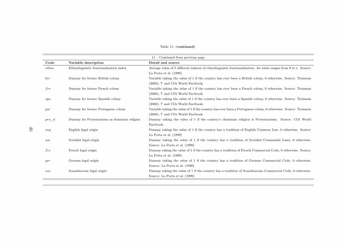
Table 11: (continued)

11 – Continued from previous page

Code Variable description Detail and source

ethno Ethnolinguistic fractionalisation index Average value of 5 different indexes of ethnolinguistic fractionalization. Its value ranges from 0 to 1. Source:

La Porta et al. (1999).

bri Dummy for former British colony Variable taking the value of 1 if the country has ever been a British colony, 0 otherwise. Source: Treisman

(2000), ? and CIA World Factbook.

fre Dummy for former French colony Variable taking the value of 1 if the country has ever been a French colony, 0 otherwise. Source: Treisman

(2000), ? and CIA World Factbook.

spa Dummy for former Spanish colony Variable taking the value of 1 if the country has ever been a Spanish colony, 0 otherwise. Source: Treisman

(2000), ? and CIA World Factbook.

por Dummy for former Portuguese colony Variable taking the value of 1 if the country has ever been a Portuguese colony, 0 otherwise. Source: Treisman

(2000), ? and CIA World Factbook.

pro_d Dummy for Protestantism as dominant religion Dummy taking the value of 1 if the country’s dominant religion is Protestantism. Source: CIA World

Factbook.

eng English legal origin Dummy taking the value of 1 if the country has a tradition of English Common Law, 0 otherwise. Source:

La Porta et al. (1999)

soc Socialist legal origin Dummy taking the value of 1 if the country has a tradition of Socialist/Communist Laws, 0 otherwise.

Source: La Porta et al. (1999)

fre French legal origin Dummy taking the value of 1 if the country has a tradition of French Commercial Code, 0 otherwise. Source:

La Porta et al. (1999)

ger German legal origin Dummy taking the value of 1 if the country has a tradition of German Commercial Code, 0 otherwise.

Source: La Porta et al. (1999)

sca Scandinavian legal origin Dummy taking the value of 1 if the country has a tradition of Scandinavian Commercial Code, 0 otherwise.

Source: La Porta et al. (1999)

40