Multivariate Input Uncertainty in Output Analysis for ...homepages.rpi.edu/~xiew3/XieBartonNelsonMultivariate_2016.pdfMultivariate Input Uncertainty in Output Analysis for Stochastic

5

Multivariate Input Uncertainty in Output Analysis for StochasticSimulation

WEI XIE, Rensselaer Polytechnic InstituteBARRY L. NELSON, Northwestern UniversityRUSSELL R. BARTON, The Pennsylvania State University

When we use simulations to estimate the performance of stochastic systems, the simulation is often driven byinput models estimated from finite real-world data. A complete statistical characterization of system perfor-mance estimates requires quantifying both input model and simulation estimation errors. The componentsof input models in many complex systems could be dependent. In this paper, we represent the distribution ofa random vector by its marginal distributions and a dependence measure: either product-moment or Spear-man rank correlations. To quantify the impact from dependent input model and simulation estimation errorson system performance estimates, we propose a metamodel-assisted bootstrap framework that is applicableto cases when the parametric family of multivariate input distributions is known or unknown. In either case,we first characterize the input models by their moments that are estimated using real-world data. Then,we employ the bootstrap to quantify the input estimation error, and an equation-based stochastic krigingmetamodel to propagate the input uncertainty to the output mean, which can also reduce the influence ofsimulation estimation error due to output variability. Asymptotic analysis provides theoretical support forour approach, while an empirical study demonstrates that it has good finite-sample performance.

Categories and Subject Descriptors: I.6.6 [Simulation and Modeling]: Simulation Output Analysis

General Terms: Algorithms, Experimentation

Additional Key Words and Phrases: Bootstrap, confidence interval, Gaussian process, multivariate inputuncertainty, NORTA, output analysis

ACM Reference Format:Wei Xie, Barry L. Nelson, and Russell R. Barton. 2016. Multivariate input uncertainty in output analysisfor stochastic simulation. ACM Trans. Model. Comput. Simul. 27, 1, Article 5 (October 2016), 22 pages.DOI: http://dx.doi.org/10.1145/2990190

1. INTRODUCTION

Stochastic simulation is used to estimate the performance of complex systems that aredriven by random input models. The distributions of these input models are often esti-mated from finite real-world data. Therefore, a complete statistical characterization ofstochastic system performance requires quantifying both input and simulation estima-tion error. Ignoring either source of uncertainty could lead to unfounded confidence inthe system performance estimate. In this paper, we focus on the system mean response,

This is based on work supported by the National Science Foundation under Grant No. CMMI-1068473.Authors’ addresses: W. Xie (corresponding author), Department of Industrial and Systems Engineering,Rensselaer Polytechnic Institute, Troy, NY 12180-3590; email: [email protected]. B. L. Nelson, Department ofIndustrial Engineering and Management Sciences, Northwestern University, Evanston, IL 60208; email:[email protected]. R. R. Barton, Smeal College of Business, Pennsylvania State University, Uni-versity Park, PA 16802; email: [email protected] to make digital or hard copies of part or all of this work for personal or classroom use is grantedwithout fee provided that copies are not made or distributed for profit or commercial advantage and thatcopies show this notice on the first page or initial screen of a display along with the full citation. Copyrights forcomponents of this work owned by others than ACM must be honored. Abstracting with credit is permitted.To copy otherwise, to republish, to post on servers, to redistribute to lists, or to use any component of thiswork in other works requires prior specific permission and/or a fee. Permissions may be requested fromPublications Dept., ACM, Inc., 2 Penn Plaza, Suite 701, New York, NY 10121-0701 USA, fax +1 (212)869-0481, or [email protected]© 2016 ACM 1049-3301/2016/10-ART5 $15.00DOI: http://dx.doi.org/10.1145/2990190

ACM Transactions on Modeling and Computer Simulation, Vol. 27, No. 1, Article 5, Publication date: October 2016.

5:2 W. Xie et al.

and our approach can be applied to other performance estimates, for example, varianceand probabilities.

The choice of input models directly impacts the system performance estimates. Aprevalent practice is to model the input processes as a collection of independent andidentically distributed (i.i.d.) univariate distributions. However, considering that com-ponents of real inputs could be dependent, these simple models do not always faithfullyrepresent the physical processes. For example, in a project planning network, the ac-tivity durations for different tasks could be correlated if they are affected by the samenuisance factors, for example, weather conditions. In a supply chain system, the de-mands of a customer for different products, for example, low-fat and whole milk, couldbe related. In financial risk management, strong dependence between assets in a port-folio could occur if their values are derived from common underlying assets. And ina production-scheduling problem, the operation times for a particular job at a seriesof processing stations could be dependent. Ignoring such dependence can lead to poorestimates of system performance. Thus, it is desirable to build input models that canfaithfully capture the dependence through joint rather than univariate input distribu-tions. In this paper we account for input models with random-vector distributions anddo not consider time-series input processes.

Biller and Ghosh [2006] reviewed various approaches to construct joint input distri-butions. Considering the amount of information needed to specify the joint distribution,almost all these methods suffer from some serious drawbacks. In light of this difficulty,most input-modeling research focuses on methods that match only certain key prop-erties of the input models, including the marginal distributions and some dependencemeasure.

We assume that dependent input models are characterized by their marginal distribu-tions and a dependence measure. Specifically, the marginal distributions have knownparametric families with parameter values unknown. The dependence between dif-ferent components of input models can be measured by various criteria [Biller andGhosh 2006]. We focus on product-moment and Spearman rank correlations in thispaper. Product-moment correlation measures linear dependence and it is widely usedin engineering applications. The definition of product-moment correlation needs thevariances of the components to be finite. Thus, we also include the use of Spearmanrank correlation as a dependence measure, which finds wide application in businessstudies, for example, decision and risk analysis [Clemen and Reilly 1999]. Instead ofmeasuring linear dependence, the Spearman rank correlation captures monotonic, pos-sibly nonlinear dependence between different components of input models; it does notrequire the variances of the components to be finite. Further, since it is based on ranks,it is not sensitive to observation outliers. Notice that in general, dependence may bemore than just pairwise and monotonic, in which case a more complex characterizationmay be needed [Wu and Mielniczuk 2010].

Since marginal distributions and dependence measures are estimated from real-world data, their estimation error is called input uncertainty. Therefore, when weuse the simulation outputs to estimate system performance, there are two sourcesof uncertainty: input and simulation error. To quantify the overall uncertainty aboutthe system performance estimate, we build on Xie et al. [2015], which proposed ametamodel-assisted bootstrapping approach to form a confidence interval (CI) ac-counting for the impact of input and simulation uncertainty. Further, a variance de-composition was proposed to estimate the relative contribution of input to overalluncertainty. However, our previous study in Xie et al. [2015] was based on the as-sumption that the input distributions are univariate and mutually independent. Theindependence assumption does not hold in general for input models in many stochasticsystems.


Multivariate Input Uncertainty in Output Analysis for Stochastic Simulation 5:3

This is a significant enhancement of Xie et al. [2015]. To efficiently and correctlyaccount for uncertainty in multivariate input models, we introduce a more generalmetamodel-assisted bootstrapping framework; it can quantify the impact of dependentinput uncertainty and simulation estimation error on system performance estimateswhile also reducing the influence of simulation estimation error due to finite simulationeffort.

Suppose that input models are characterized by marginal distributions and a cor-relation matrix, and that the parameters are specified by a vector of moments, calledmoment-based parameters; see Section 4.1 for the detailed definition. In this paper, weconsider two cases. First, when the full parametric joint distribution is known exceptfor the marginal distribution parameters and a correlation matrix, then we work withthe joint distribution directly, for example, multivariate Pearson distribution. Second,when the parametric joint input distribution is unknown, we construct the joint distri-bution by using the flexible NORmal To Anything (NORTA) representation [Cario andNelson 1997]. Since moment-based parameters are estimated with real-world data, thebootstrap is used to quantify the input estimation error, and an equation-based stochas-tic kriging (SK) metamodel propagates the input uncertainty to the output mean. Wecan derive a CI that accounts for both simulation and input uncertainty by using thisgeneralized metamodel-assisted bootstrapping approach. Therefore, our approach al-lows us to do statistical uncertainty analysis for stochastic systems with dependencein the input models.

There are two central contributions of this : first, we generalize the metamodel-assistedbootstrap framework [Xie et al. 2015] to stochastic simulation with dependent inputmodels; second, we propose a rigorous analysis for cases where the dependence is mea-sured by product-moment or Spearman rank correlation.

The next section describes other research on dependent input modeling and inputuncertainty analysis. This is followed by a formal description of the problem of interestin Section 3. In Section 4, we propose a generalized metamodel-assisted bootstrap-ping framework and provide a procedure to build a CI accounting for both input andsimulation estimation error on system mean performance estimates. Our approach issupported by asymptotic analysis. We then report results of finite sample behaviorfrom an empirical study in Section 5 and conclude in Section 6. All proofs are in theOnline Appendix.

2. BACKGROUND

For stochastic simulations, various approaches to account for input uncertainty havebeen proposed; see Barton [2012] and Song et al. [2014] for reviews. The methods can bedivided into Bayesian and frequentist approaches, which have their underlying meritsand limitations [Xie et al. 2014a].

Johnson [1987] reviewed various parametric joint distributions useful in the simu-lation that can be parameterized by marginal moments and a correlation matrix. Forexample, the multivariate Johnson translation system matches the first four momentsfor each marginal distribution and a correlation matrix. A flexible bivariate Gammadistribution proposed in Schmeiser and Lal [1982] allows any Gamma marginal distri-butions and associated correlations. The multivariate Pearson type II distribution ischaracterized by the marginal means and a covariance matrix.

When only the marginal distribution families are known, Cario and Nelson [1997]proposed a flexible NORTA distribution to represent and generate random vectorswith almost arbitrary marginal distributions and product-moment correlation matrix.Clemen and Reilly [1999] used NORTA to represent the dependent input models fordecision and risk analysis with dependence measured by Spearman’s and Kendall’srank correlations.


5:4 W. Xie et al.

Biller and Corlu [2011] proposed a Bayesian approach to account for the param-eter uncertainty for dependent input models. Correlated inputs are modeled withNORTA and the dependence is measured by product-moment correlation. The un-certainty around the NORTA distribution parameters estimated from real-world datais quantified by posterior distributions. For complex stochastic systems with a largenumber of correlated inputs, a fast algorithm draws samples from these posterior dis-tributions to quantify the input uncertainty. Then, the direct simulation method isused to propagate the input uncertainty to the output mean by running simulations ateach sample point, which could be computationally expensive for complex simulatedsystems. Further, the direct simulation method does not incorporate the simulationuncertainty into the Bayesian formulation; see Xie et al. [2014a].

Direct bootstrapping uses bootstrap resampling of the real-world data to representthe input uncertainty and propagates it to the output mean by direct simulation [Bartonand Schruben 1993, 2001]; Barton 2007; Cheng and Holland 1997]. Compared withthe Bayesian approaches, the direct bootstrap can be adapted to any input modelswithout additional analysis, and it does not need to resort to computationally expensiveapproaches to draw posterior samples to quantify the input uncertainty. However, directsimulation cannot efficiently use the computational budget to reduce the impact fromsimulation estimation error. Further, since the statistic that is bootstrapped is therandom output of a simulation, it is not a smooth function of input data; this violatesthe asymptotic validity of the bootstrap.

The metamodel-assisted bootstrapping approach was introduced by Barton et al.[2014]. The input uncertainty is measured by bootstrapping and an equation-basedSK metamodel propagates the input uncertainty to the output mean. This approachaddresses some of the shortcomings of the direct bootstrap. Specifically, the metamodelcan reduce the impact of simulation estimation error. Further, metamodeling makes thebootstrap statistic a smooth function of the input data so that the asymptotic validityconcerns faced by the direct bootstrap method disappear. However, Barton et al. [2014]assumed that the simulation budget is not tight and the metamodel uncertainty can beignored. If the true mean response surface is complex, especially for high-dimensionalproblems with many input distributions, and the computational budget is tight, thenthe impact of metamodel uncertainty can no longer be ignored.

The metamodel-assisted bootstrapping approach was improved in Xie et al. [2015] tobuild a CI accounting for the impact from both input and metamodel uncertainty on thesystem mean estimates. Further, a variance decomposition was proposed to estimatethe relative contribution of input to overall uncertainty, which is very useful for decisionmakers to determine where to put more effort to reduce the estimator error. Themetamodel-assisted bootstrapping approach demonstrates robust performance evenwhen there is a tight computational budget and simulation estimation error is large.However, Xie et al. [2015] is based on the assumption that input models are a collectionof mutually independent univariate distributions.

The success of metamodel-assisted bootstrapping for stochastic simulations withindependent univariate input distributions in Xie et al. [2015] motivates us to extendit to more complex cases with dependence in the input models.

3. PROBLEM STATEMENT

The stochastic simulation output is a function of random numbers and the input modeldenoted by F. For notation simplification, we do not explicitly include the randomnumbers. The output from the jth replication of a simulation with input model F canbe written as

Yj(F) = μ(F) + ε j(F),



where μ(F) = E[Yj(F)] denotes the unknown output mean and ε j(F) represents thesimulation error with mean zero. Notice that the simulation output depends on thechoice of input model.

In general, F could be composed of mutually independent univariate and multi-variate joint distributions. For simplification, suppose that F is composed of a sin-gle multivariate distribution with dimension d > 1. The marginal distributions ofF are denoted by {F1, F2, . . . , Fd}. In this paper, we focus on continuous marginaldistributions.

Suppose that F is characterized by the marginal distributions and a dependencemeasure: either product-moment or Spearman rank correlation matrix. Specifically,let a d × 1 random vector X ∼ F having d × d product-moment and Spearman rankcorrelation matrix denoted, respectively, by ρX and RX with

ρX(i, j) = corr(Xi, Xj) = Cov(Xi, Xj)√Var(Xi)Var(Xj)

,

RX(i, j) = corr(Fi(Xi), Fj(Xj)) = E[Fi(Xi)Fj(Xj)] − E[Fi(Xi)]E[Fj(Xj)]√Var(Fi(Xi))Var(Fj(Xj))

for i, j = 1, 2, . . . , d. Suppose these correlation matrices are positive definite. Sincethe correlation matrices are symmetric and their diagonal terms are 1, we can viewa d × d correlation matrix as an element of d∗ ≡ d(d − 1)/2 dimensional Euclideanspace. Therefore, the product-moment and Spearman rank correlation matrix can beuniquely specified by d∗ × 1 vectors denoted by Vρ

X and VRX , respectively.

We assume that the families of marginal distributions {F1, F2, . . . , Fd} are known,but not their parameter values. Let an hi ×1 vector θθθ i denote the unknown parametersfor the ith marginal distribution Fi. By stacking θθθ i with i = 1, 2, . . . , d together, wehave a d† × 1 dimensional parameter vector θθθ� ≡ (θθθ�

1 , θθθ�2 , . . . , θθθ�

d ) with d† ≡ ∑di=1 hi.

Input models characterized by marginal distributions and correlation matrices canbe specified by ϑϑϑ ≡ (θθθ ; VX) that includes d′ ≡ d† + d∗ elements, where VX = Vρ

X or VRX .

We call ϑϑϑ the input model parameters. By abusing notation, we can rewrite μ(F) asμ(ϑϑϑ). The true input parameters ϑϑϑc are unknown and estimated from finite samples ofreal-world data. Thus, our goal is finding a (1 − α)100% CI [QL, QU ] such that

Pr{μ(ϑϑϑc) ∈ [QL, QU ]} = 1 − α. (1)

The unknown input model parameters are estimated by the real-world data, denoted

by Xm ≡ {X(1), X(2), . . . , X(m)}, where the d × 1 random vector X(i) i.i.d∼ Fc with i =1, 2, . . . , m. Under the assumption that the first hi marginal moments are finite for i =1, 2, . . . , d, we estimate marginal distribution parameters by the moment estimators,denoted by θθθm [Xie et al. 2015]. The usual estimators for the product-moment andSpearman rank correlations are

ρX,m(i, j) =∑m

k=1

(X(k)

i − Xi)(

X(k)j − Xj

)/(m− 1)

Si Sj(2)

RX,m(i, j) =∑m

k=1

(r(X(k)

i ) − r(Xi))(

r(X(k)j ) − r(Xj)

)√[ ∑mk=1

(r(X(k)

i ) − r(Xi))2] · [ ∑m

k=1

(r(X(k)

j ) − r(Xj))2] (3)

for i, j = 1, 2, . . . , d, where Xi = ∑mk=1 X(k)

i /m and S2i = ∑m

k=1

(X(k)

i − Xi)2

/(m − 1).We denote the rank function by r(·) ≡ rank(·). In this paper, we use the uprank to


5:6 W. Xie et al.

estimate the Spearman rank correlations. It is defined by r(X(k)i ) ≡ ∑m

j=1 I(X( j)i ≤ X(k)

i )and r(Xi) = ∑m

k=1 r(X(k)i )/m with I(·) denoting an indicator function. Then, based on

Equations (2) and (3), we can find corresponding correlation estimators Vρ

X,m and VRX,m.

Given the input-model parameter estimator ϑϑϑm = (θθθm; Vρ

X,m) or (θθθm; VRX,m) that is a

function of real-world data Xm, its sampling distribution can be used to quantify inputuncertainty.

The impact of input uncertainty on the system mean performance estimate is quan-tified by the sampling distribution of μ(ϑϑϑm). Further, since the underlying responsesurface μ(·) is unknown, at any ϑϑϑ , let μ(ϑϑϑ) denote the corresponding mean responseestimator. Thus, there are both input and simulation estimation errors in the systemmean performance estimates.

For stochastic systems with dependent input models, our objective is to create anapproach to quantify the overall impact of both input and simulation estimation erroron system mean performance estimates and then build a CI satisfying Equation (1).Further, since each simulation run could be computationally expensive and we may havea tight computational budget, we want to reduce the influence of simulation estimationerror.

4. METAMODEL-ASSISTED BOOTSTRAPPING FRAMEWORK

For problems with parametric input distributions that are univariate and mutually in-dependent, the metamodel-assisted bootstrapping framework was used to account forthe impact of both input and simulation estimation errors on the system performanceestimates in Xie et al. [2015]. In this section, we generalize the metamodel-assistedbootstrapping approach for stochastic simulations with dependence in the inputmodels.

To make this section easy to follow, we start with an overall description of the general-ized metamodel-assisted bootstrapping framework. We employ the bootstrap to capturethe estimation error of moment-based input parameters in Section 4.1, and propagatethe input uncertainty to the output mean by using an equation-based stochastic krigingmetamodel that is built based on the simulation outputs at a few well-chosen designpoints; see Section 4.3. At each design point, we need to construct a full joint input dis-tribution, generate samples of X to drive simulations, and estimate the system meanresponses. We consider cases with the family of parametric joint distribution knownor unknown, respectively, in Section 4.2. Then, since both simulation and metamodeluncertainty can be estimated using properties of an SK metamodel, we propose aprocedure to deliver a CI that accounts for both simulation and input uncertainty inSection 4.4. Asymptotic analysis provides theoretical support for our approach.

Notice that direct simulation, by running the simulations at each bootstrappedsample of input moments to estimate the system performance, could be used topropagate the input uncertainty to the output. Our previous study [Xie et al. 2014a]demonstrates the advantages by using an SK metamodel over direct simulation.Given a finite simulation budget, the SK metamodel efficiently reduces the impactof simulation estimation uncertainty. In addition, bootstrap consistency requiresthe statistic to be a smooth function of the data. Direct simulation violates thisrequirement. This issue does not exist in our metamodel-assisted bootstrappingapproach; see Barton et al. [2014] and Xie et al. [2015].

4.1. Bootstrap for Input Uncertainty

In this section, we describe how to employ the bootstrap to quantify the input un-certainty. The way we choose to represent input models plays an important role in



the implementation of metamodel-assisted bootstrapping. Moment-based parameters,denoted by M, are used to characterize the input model with dependence. Insteadof using the natural parameters θθθ to characterize the marginal distributions, we canuse moments; see Barton et al. [2014] for an explanation. Suppose that the para-metric marginal distribution Fi can be uniquely characterized by its first hi finitemoments denoted by the hi × 1 vector ψψψ i for i = 1, 2, . . . , d. By stacking ψψψ i withi = 1, 2, . . . , d together, we have a d† × 1 dimensional vector of marginal momentsψψψ� ≡ (ψψψ�

1 ,ψψψ�2 , . . . ,ψψψ�

d ). Therefore, the input models can be characterized by the col-lection of moments M = (ψψψ ; VX) with VX = Vρ

X or VRX . Suppose there is a one-to-one

continuous mapping between marginal moments and parameters, denoted by θθθ = h(ψψψ).Thus, the input parameters ϑϑϑ and moments M are interchangeable. Abusing notationagain, we rewrite μ(ϑϑϑ) as μ(M).

The true moments of dependent input models, denoted by Mc, are unknown andestimated based on a finite sample Xm. Specifically, we use standardized sample mo-ments as estimators for marginal distributions, denoted by ψψψm; see Xie et al. [2015].The correlation estimator Vρ

X,m or VRX,m is obtained by using Equation (2) or (3). The

estimation error of input models can be quantified by the sampling distribution ofMm = (ψψψm; Vρ

X,m) or (ψψψm; VRX,m), denoted by Fc

Mm. Therefore, the impact of input uncer-

tainty on the system mean performance estimate can be measured by the samplingdistribution of μ(Mm) with Mm ∼ Fc

Mm.

Since it could be hard to derive the sampling distribution FcMm

, we use bootstrap re-sampling to approximate it [Shao and Tu 1995]. Let A ≡ {1, 2, . . . , m}. Implementationof bootstrap resampling in the metamodel-assisted bootstrapping is as follows:

(1) Draw m samples with replacement from set A and obtain bootstrapped indexes{i1, i2, . . . , im}; choose corresponding samples from real-world data Xm and getX(1)

m ≡ {X(i1), X(i2), . . . , X(im)}. Use X(1)m to calculate the bootstrapped moment esti-

mate, denoted by M(1)m ≡ (ψψψ

(1)m ; (Vρ

X,m)(1)) or (ψψψ(1)m ; (VR

X,m)(1)).(2) Repeat Step (1) for B times to generate M(b)

m with b = 1, 2, . . . , B.

The bootstrap resampled moments are drawn from the bootstrap distribution, denotedby FMm(·|Xm), with Mm ∼ FMm(·|Xm). For estimation of a percentile CI quantifying theimpact of input uncertainty, B is recommended to be a few thousand; see Xie et al.[2014a]. In this paper, adenotes a quantity estimated from real-world data, while a˜denotes a quantity estimated from bootstrapped data.

Theorem 4.1 shows that when the amount of real-world data increases to infinity,the bootstrap provides a consistent estimator for the true input moments Mc.

THEOREM 4.1. Suppose the following conditions hold:

(1) We have X(k) i.i.d∼ Fc with k = 1, 2, . . . , m.(2) The marginal distribution Fc

i is uniquely characterized by its first hi moments andit has finite first 4hi moments for i = 1, 2, . . . , d.

(3) E(X4i X4

j ) < ∞ for i, j = 1, 2, . . . , d.

Then, as m → ∞, the bootstrap moment estimator Mm converges a.s. to the true momentsMc.

The proof of Theorem 4.1 is provided in the Online Appendix.Notice that under some situations, such as when the input model does not have

enough finite moments, the normal approximation obtained by the Central Limit The-orem may perform better than the bootstrap; see Hall [1988]. For this case, we could


5:8 W. Xie et al.

easily extend our framework by using the normal approximation to quantify the inputuncertainty.

4.2. Construction of Joint Input Distributions

Given feasible moment-based parameters, we describe the procedure to construct thejoint input distribution in this section. We first consider the case when the full paramet-ric joint distribution is known except the marginal parameters and a correlation matrixin Section 4.2.1. Then, when the parametric family is unknown, we use a NORTA rep-resentation to construct the joint distribution in Section 4.2.2. Notice that unless thetrue distribution is NORTA, there is unmeasured error due to incorrect input models.That error is not addressed in this paper.

4.2.1. Parametric Joint Input Distributions. In this section, we consider multivariate para-metric input distributions F with the distribution family known. The input model isspecified by marginal parameters θθθ and a correlation matrix ρX; see Schmeiser andLal [1982] and Johnson [1987] for multivariate families useful in simulation. The un-derlying correct parameters (θθθ c; (Vρ

X)c) are unknown and estimated by finite real-worlddata.

We use a multivariate Pearson type II distribution [Johnson 1987] as an illustrativeexample. It has the density function

f (x) = �(d/2 + κ + 1)�(κ + 1)πd/2 |�|−1/2[1 − (x − μμμ)′�−1(x − μμμ)]κ .

Suppose that the shape parameter κ is given. Then, the Pearson type II distribution isspecified by parameters μμμ and � with

E(X) = μμμ and Cov(X) = �

2κ + d + 2.

It can also be specified by the moment vector M, including the first two marginalmoments and the correlation vector Vρ

X.For a general parametric joint distribution F that could be specified by marginal

parameters θθθ and a correlation matrix ρX, Theorem 4.2 shows that for any momentvector M in a small neighborhood centered at Mc, we could find a feasible multivariateparametric distribution F.

THEOREM 4.2. Let F be a parametric multivariate input distribution specified bymarginal parameters θθθ and a correlation matrix ρX. Let �� ⊆ �d†

be the feasible domainfor marginal distribution parameters θθθ . Suppose the following conditions hold:

(1) Any parameter vector ϑϑϑ with θθθ ∈ �� and positive semidefinite ρX has a feasiblemultivariate parametric joint distribution F.

(2) θθθ c is an interior point in ��, and ρcX is positive definite.

(3) There is a one-to-one continuous mapping between marginal moments and param-eters, θθθ = h(ψψψ).

Then the true moment vector Mc = (ψψψc; (Vρ

X)c) is an interior point of the feasible region:in the d′ dimensional Euclidean space, there exists a constant δ > 0 such that anymoment combination M in the open ball Bδ(Mc) has a feasible parametric multivariatedistribution F.

The proof of Theorem 4.2 is provided in the Online Appendix.Notice that if the marginals have the same family, we may find an existing parametric

multivariate distribution to use; see Johnson [1987]. For marginals having differentfamilies, we typically cannot use a standard multivariate parametric distribution, and



we need to consider the transformation-based approaches, for example, NORTA andmultivariate Johnson distributions.

4.2.2. NORTA Representation. In this section, suppose that the parametric family ofjoint input distribution F is unknown. Given the partial characterization specified bymarginal distributions and a pairwise dependence measure, either product-momentor Spearman rank correlations, we now describe how to employ the NORTA repre-sentation for constructing the joint distributions and generating samples of randomvector X.

To find a NORTA representation for F, we represent X as a transformation of ad-dimensional standard multivariate normal (MVN) vector Z = (Z1, Z2, . . . , Zd)� withproduct-moment correlation matrix denoted by ρZ,

X� = (F−1

1 [�(Z1);θθθ1], F−12 [�(Z2);θθθ2], . . . , F−1

d [�(Zd);θθθd]), (4)

where �(·) denotes the cdf for the standard normal distribution. If the marginal distri-bution families are given, as we assume here, then the NORTA representation for Fcan be specified by (θθθ, ρZ). For a standard normal random vector Z, there is a closed-form relation between product-moment correlation ρZ and Spearman rank correlationRZ [Clemen and Reilly 1999]:

RZ(i, j) = 6π

sin−1(

ρZ(i, j)2

), (5)

with i, j = 1, 2, . . . , d.Since the NORTA implementations for cases where the dependence is measured

by Spearman rank and product-moment correlations are different, we describe themseparately.

If the dependence in the input models is measured by the Spearman rank correla-tion, we have RX = RZ since it is invariant under monotone one-to-one transformationF−1

i [�(·)] for i = 1, 2, . . . , d. Therefore, given moment-based parameters M = (ψψψ ; VRX ),

we can find ϑϑϑ = (θθθ ; VRX ) by moment matching. The procedure to find a NORTA repre-

sentation and generate samples for X is as follows:

(1) From VRX , get the Spearman rank correlation matrix for Z, RZ = RX, and obtain

corresponding product-moment correlation ρZ(i, j) = 2 sin(π RZ(i, j)/6) for i, j =1, 2, . . . , d.

(2) Generate Zi.i.d.∼ MVN(0, ρZ) and obtain X by using Equation (4).

By repeating this procedure, we generate samples for X, use them to drive simulations,and estimate the mean response μ(M).

Notice that when we use Spearman rank correlation to measure the pairwise depen-dence between the components of input models, the choice of marginal distributionsand correlation is separable. However, for F specified by a combination of feasibleθθθ and a positive definite Spearman rank correlation matrix RX, we may not find aNORTA representation because the nonlinear transformation of positive definite RZ,ρZ(i, j) = 2 sin[π RZ(i, j)/6], could lead to a nonpositive definite correlation matrix ρZ;see Ghosh and Henderson [2002a] and Li and Hammond [1975].

If the dependence between the components of input models is measured by product-moment correlation, then the procedure to find a NORTA representation becomes morecomplex because the choice of marginal distributions influences the feasibility of thecorrelation matrix. Specifically, there is a pairwise relation between product-moment


5:10 W. Xie et al.

correlation matrices of X and Z:

ρX(i, j) = Cij[ρZ(i, j);θθθ ]

≡∫ ∫

F−1i [�(zi);θθθ i]F−1

j [�(zj);θθθ j]ϕρZ(i, j)(zi, zj)dzidzj − E(Xi)E(Xj)√Var(Xi)Var(Xj)

, (6)

where ϕρZ(i, j) denotes the standard bivariate normal density with correlation ρZ(i, j)and Cij denotes a pairwise transformation from ρZ(i, j) to ρX(i, j) for i, j = 1, 2, . . . , d.Given θθθ and ρX, we solve d∗ correlation-matching Equation (6) to find ρZ. UnlikeSpearman rank correlation, the marginal distributions characterized by parame-ters θθθ play an important role in determining the value and feasibility of correlationmatrix ρZ.

Given M = (ψψψ ; Vρ

X), we can find ϑϑϑ = (θθθ ; Vρ

X) by moment matching. If there exists afeasible NORTA representation, the procedure to find it and generate samples for X isas follows:

(1) Given Vρ

X, solve Equation (6) for correlation matrix ρZ.

(2) Generate Zi.i.d.∼ MVN(0, ρZ) and obtain X by using Equation (4).

By repeating this procedure, we generate samples for X and then use them to drivesimulations to estimate μ(M). When we solve for ρZ in Step (1), typically there isno closed-form analytical solution except for some special marginal distributions, forexample, uniform distribution, and we need to resort to numerical search to obtain ρZ.

Notice that when we use product-moment correlation to characterize the pairwisedependence between the components of input models, the nonlinear transformationbetween ρX and ρZ in Equation (6) may not guarantee the positive semidefinite propertyfor ρZ. There may not exist a NORTA representation for every feasible combination ofθθθ and positive definite ρX. Therefore, the previous procedure only works under thecondition that the correlation matrix ρZ obtained in Step (1) is positive semidefinite,which may not hold in general. Based on the study by Ghosh and Henderson [2002b],this infeasibility is more likely in high dimensions and with correlations close to ±1.When this happens, we can find a NORTA feasible correlation matrix that is closeto ρX.

If ρZ obtained by nonlinear transformation ρZ(i, j) = 2 sin[π RZ(i, j)/6] or by solvingd∗ in Equation (6) is positive semidefinite, ϑϑϑ = (θθθ ; VX) with VX = VR

X or Vρ

X is calledNORTA feasible; otherwise, it is called NORTA infeasible. Theorem 4.3 gives a propertyof the NORTA feasible region: if the true moment combinationMc has a NORTA feasiblerepresentation with positive definite ρc

Z, then there exists a neighborhood centered at Mc

in the d† + d∗ dimensional Euclidean space such that every moment combination Min the neighborhood has a NORTA feasible representation. This property is usefulwhen we show the asymptotic consistency of the CI built by the metamodel-assistedbootstrapping to quantify both input and simulation uncertainty in Section 4.4.

THEOREM 4.3. Let �� ⊆ �d†be the feasible domain for marginal distribution parame-

ters θθθ and suppose θθθ c is an interior point in ��. Suppose there is one-to-one continuousmapping between marginal moments ψψψ i and parameters θθθ i for i = 1, 2, . . . , d. Supposethe following conditions hold:

(1) Fc has a NORTA feasible representation (θθθ c, ρcZ) with ρc

Z positive definite.(2) At any x, the marginal distributions Fi(x;θθθ i), density functions fi(x;θθθ i), and inverse

distributions F−1i (x;θθθ i) are continuously differentiable over θθθ i for i = 1, 2, . . . , d on

��.



(3) For any θθθ ∈ ��, the marginal cdfs F1(x;θθθ1), F2(x;θθθ2), . . . , Fd(x;θθθd) are continuousand strictly increasing in x.

Then the true moment vector Mc = (ψψψc; VcX) with VX = Vρ

X or VRX is an interior point

of the NORTA feasible region: in the d† + d∗ dimensional Euclidean space, there existsa constant δ > 0 such that every moment combination M in the open ball Bδ(Mc) has aNORTA feasible representation.

The proof of Theorem 4.3 is provided in the Online Appendix.

4.3. Stochastic Kriging Metamodel

In the metamodel-assisted bootstrapping framework, after quantifying the input uncer-tainty with the bootstrap as described in Section 4.1, an equation-based SK metamodelintroduced by Ankenman et al. [2010] is used to propagate the input uncertainty to theoutput mean. The succinct review of SK in this section is based on Ankenman et al.[2010].

Dependent input models characterized by finite moment-based parameters M com-posed of marginal standard moments and component-pairwise correlations can be inter-preted as a location x in a d′ = (d† +d∗) dimension space. The p-norm distance could beused to measure the difference between moment-based parameters x and x′ defined by

d(x, x′) = ‖x�ζζζx′‖1/pp =

⎡⎣ d′∑j=1

ζ j(xj − x′

j

)p

⎤⎦1/p

, (7)

with p ≥ 1, where x is a d′ × 1 moment vector and ζζζ denotes a d′ × d′ diagonal matrixwith nonnegative diagonal terms ζ1, ζ2, . . . , ζd′ . In this paper, the distance betweendifferent estimates of input models is measured by a weighted Euclidean distanceon moment-based parameters with p = 2. Since the marginal moments and pairwisecorrelations could have different impacts on the system performance, the weights ζζζquantify their relative effects. For example, if the marginal moments have dominanteffects, the corresponding weights tend to be higher.

This distance measure was used to measure the difference between moment es-timates for univariate parametric input models in Barton et al. [2014]. In terms ofdistance measures for a correlation matrix, Higham [2002] used weighted Euclideandistance, while Ghosh and Henderson [2002b] used other norms, including L1 and L∞.We choose the weighted Euclidean distance because each individual correlation canmatter and different correlation elements could have different impacts on the systemmean performance. The distance measures L1 and L∞ do not capture that. Notice thatsince the correlation matrix is required to be positive semidefinite, there exist implicitconstraints on the elements of the correlation matrix.

The input models with closer moments tend to have closer mean responses. Supposethat the underlying true (but unknown) response surface is a continuous function ofmoment-based parameters x and μ(·) is a realization of a stationary Gaussian Process(GP). We model the simulation output Y by

Yj(x) = β0 + W(x) + ε j(x). (8)

This model includes two sources of uncertainty: the simulation output uncertainty ε j(x)and mean response uncertainty characterized by the GP W(x). For many, but not all,simulation settings, the output is an average of a large number of more basic outputs,so a normal approximation can be applied: ε(x) ∼ N(0, σ 2

ε (x)). For example, when westudy the steady-state expected waiting time in a queue, each simulation output is theaverage of waiting times for many customers.


5:12 W. Xie et al.

Since stochastic systems with dependent input models having similar key prop-erties tend to have close mean responses, a zero-mean, second-order stationary GPW(·) is used to account for this spatial dependence. Therefore, the uncertainty aboutthe unknown true response surface μ(x) is represented by a GP M(x) ≡ β0 +W(x) (notethat β0 can be replaced by a more general trend term f(x)�β). Its spatial dependenceis characterized by the covariance function, �(x, x′) = Cov[W(x), W(x′)] = τ 2γ (x − x′),where τ 2 denotes the variance and γ (·) is a correlation function that depends only onthe distance x − x′. Based on prior information about the smoothness of μ(·), we canchoose the form of correlation function [Xie et al. 2010]. Considering that mean responsesurfaces for most system engineering problems have a high order of smoothness andGaussian correlation function demonstrates good performance [Mukhopadhyay et al.2016], we use the product-form Gaussian correlation function

γ (x − x′) = exp(

−d′∑

j=1

ζ j(xj − x′j)

2)

(9)

for the empirical evaluation in Section 5. In SK, the weights ζζζ = (ζ1, ζ2, . . . , ζd′ ) arealso called correlation parameters that quantify the relative effects of elements in themoment-based parameters on the system mean response. Before having any simulationresult, the uncertainty about μ(x) can be represented by a Gaussian process M(x) ∼GP(β0, τ

2γ (x − x′)).To reduce the uncertainty about μ(x), we choose an experiment design consist-

ing of pairs D ≡ {(xi, ni), i = 1, 2, . . . , K} with (xi, ni) denoting the location and thenumber of replications at the ith design point. The simulation outputs at D areYD ≡ {(Y1(xi), Y2(xi), . . . , Yni (xi)); i = 1, 2, . . . , K} and the sample mean at designpoint xi is Y (xi) = ∑ni

j=1 Yj(xi)/ni. Let the sample means at all K design points beYD = (Y (x1), Y (x2), . . . , Y (xK))T and its variance be represented by a K × K diago-nal matrix C = diag{σ 2

ε (x1)/n1, σ2ε (x2)/n2, . . . , σ

2ε (xK)/nK} because the use of common

random numbers is detrimental to prediction [Chen et al. 2012].The simulation outputs YD and spatial dependence characterized by the covariance

function �(·, ·) can be used to improve system mean prediction at any fixed point x.Specifically, let � be the K × K spatial covariance matrix of the design points and let�(x, ·) be the K × 1 spatial covariance vector between each design point and x. If theparameters (τ 2, ζζζ , C) are known, then the metamodel uncertainty can be characterizedby a refined GP Mp(x) that denotes the conditional distribution of M(x) given allsimulation outputs,

Mp(x) ∼ GP(mp(x), σ 2p(x)), (10)

where mp(·) is the minimum mean squared error (MSE) linear unbiased predictor

mp(x) = β0 + �(x, ·)�(� + C)−1(YD − β0 · 1K×1), (11)

and the corresponding variance is

σ 2p(x) = τ 2 − �(x, ·)�(� + C)−1�(x, ·) + η�[1�

K×1(� + C)−11K×1]−1η, (12)

where β0 = [1�K×1(� + C)−11K×1]−11�

K×1(� + C)−1YD and η = 1 − 1�K×1(� + C)−1�(x, ·)

[Ankenman et al. 2010]. Notice that misspecified correlation functions could causebiased β0.

Since in reality the spatial correlation parameters τ 2 and ζζζ are unknown, maximumlikelihood estimates (MLEs) are typically used for prediction, and the sample varianceis used as an estimate for the simulation variance at design points C [Ankenman et al.



2010]. By substituting parameter estimates (τ 2, ζζζ , C) in Equations (11) and (12), wecan obtain the estimated mean mp(x) and variance σ 2

p(x). Thus, the metamodel we useis μ(x) = mp(x) with variance estimated by σ 2

p(x).In our study, we do not account for the estimation error of SK parameters (τ 2, ζζζ , C).

This is common in the kriging literature because fully including the effect of theseparameters’ estimation error would make the distribution of SK metamodel M(·) math-ematically and computationally intractable. The impact of SK parameter estimationuncertainty on the metamodel fit in a general situation has not been comprehensivelystudied. The studies in Das et al. [2012] and Bachoc [2013] show the asymptotic con-sistency of kriging parameter estimates via weighted least square (WLS), MLE, orcross-validation. The studies in Xie et al. [2015] and Yin et al. [2009] indicate thatwhen we use the space-filling design with a reasonable number of design points [Joneset al. 1998; Loeppky et al. 2009] and the simulation estimation uncertainty does notdominate the information from the underlying response surface, the metamodel fitis robust to the SK parameter estimation uncertainty. This does not hold when themodel is used for extrapolation. In our study, we construct a design space that coversthe most likely bootstrapped input moments, which avoids the extrapolation issue; seeSection 4.4.

4.4. Procedure to Build a CI

Since there are both input and simulation estimation errors in the system mean perfor-mance estimates, in this section, we propose a procedure to build a CI quantifying theoverall uncertainty for μ(Mc). We show that as m, B → ∞, the CI has asymptoticallyconsistent coverage.

Based on a hierarchical sampling approach, we propose the following procedure tobuild a (1 − α)100% bootstrap percentile CI. We do bootstrapping over moment-basedparameters to quantify the input uncertainty. Since each simulation run could be ex-pensive, to efficiently propagate the input uncertainty quantified by B bootstrappedmoment samples, M(b)

m with b = 1, 2, . . . , B, to outputs, we construct an SK meta-model in Steps (1) through (3) that covers the most likely bootstrapped samples. Then,Step (4) uses the SK metamodel to propagate the input uncertainty to output means,with part (a) accounting for the input uncertainty and part (b) accounting for the simu-lation estimation uncertainty. Therefore, the CI built in Step (5) quantifies the overalluncertainty for μ(Mc) estimation.

(1) Identify a design space E for the moment-based parameters M over which to fitthe metamodel. Since the metamodel is used to propagate the input uncertaintymeasured by the bootstrapped moments Mm to the output mean, the design space ischosen to be the smallest ellipsoid covering the most likely bootstrapped moments.

(2) Use a maximin distance Latin hypercube design (LHD) to embed K design pointsinto the design space E. Assign equal replications to K design points to exhaustthe simulation budget N and obtain an experiment design D = {(M(i), n), i =1, 2, . . . , K}.

(3) At K design points, generate samples of X by using the approaches describedin Section 4.2. Use these samples to drive simulations and obtain outputs yD.Compute the sample average y(M(i)) and sample variance s2(M(i)) of the simula-tion outputs, i = 1, 2, . . . , K. Fit an SK metamodel to obtain mp(·) and σ 2

p(·) using(y(M(i)), s2(M(i)),M(i)), i = 1, 2, . . . , K; see Section 4.3.

(4) For b = 1 to B:(a) Generate bootstrap moments M(b)

m by following the procedure in Section 4.1.(b) Draw Mb ∼ N(mp(M(b)

m ), σ 2p(M(b)

m )).


5:14 W. Xie et al.

Next b:(5) Report CI: [M(�Bα

2 �), M(�B(1− α2 )�)], where, M(1) ≤ M(2) ≤ · · · ≤ M(B) are the sorted

values.

To construct the design space E for the SK metamodel, we first generate a testset of bootstrapped moments, denoted by DT , by following the procedure describedin Section 4.1. Then, we find the smallest ellipsoid E that can cover the most likelybootstrapped moments, say, 99%. The ellipsoid’s center and shape are the samplemean and covariance matrix of the elements in DT . The size of DT is determined by ahypothesis test. See Barton et al. [2014] for more detailed information. By Theorem 4.1,as m → ∞, we have a consistent moment estimator Mm

a.s.→ Mc. Thus, the design spaceE automatically shrinks to a smaller and smaller region around Mc. When m is largeenough, by Theorems 4.3 and 4.2, any M in the design space E eventually has eithera feasible NORTA representation or multivariate parametric joint distribution.

The CI [M(�Bα2 �), M(�B(1− α

2 )�)] provided by our framework characterizes the impact fromboth input and metamodel uncertainty on a system performance estimate. A variancedecomposition in Xie et al. [2015] can be used to assess their relative contributionsand guide a decision maker as to where to put more effort: if the input uncertaintydominates, then get more real-world data if possible; if the metamodel uncertaintydominates, then run more simulations; if neither dominates, then do both activities toimprove the estimation accuracy of μ(Mc).

If SK parameters (τ 2, ζζζ , C) are known and we replace Mb in Step (4.b) of the CIprocedure with Mb ∼ N(mp(M(b)

m ), σ 2p(M(b)

m )), the CI obtained is [M(�Bα2 �), M(�B(1− α

2 )�)].Theorem 4.4 shows that [M(�Bα

2 �), M(�B(1− α2 )�)] is asymptotically consistent.

THEOREM 4.4. Suppose conditions for Theorems 4.1, 4.3, and 4.2 and the followingadditional assumptions hold.

(1) ε j(x)i.i.d.∼ N(0, σ 2

ε (x)) for any x, and M(x) is a stationary, separable GP with acontinuous correlation function satisfying

1 − γ (x − x′) ≤ c|log(‖ x − x′ ‖2)|1+δ1

for all ‖ x − x′ ‖2≤ δ2 (13)

for some c > 0, δ1 > 0, and δ2 < 1, where ‖ x − x′ ‖2=√∑d′

j=1(xj − x′j)2.

(2) The input processes, simulation noise ε j(x), and GP M(x) are mutually independentand the bootstrap process is independent of all of them.

Then the interval [M(�Bα2 �), M(�B(1− α

2 )�)] is asymptotically consistent, meaning the iter-ated limit

limm→∞ lim

B→∞Pr{M(�Bα/2�) ≤ Mp(Mc) ≤ M(�B(1−α/2)�)} = 1 − α. (14)

The detailed proof of Theorem 4.4 is provided in the Online Appendix.

Remark 4.5. Theorem 4.4 is based on the assumption that the Gaussian processcan correctly characterize the estimation uncertainty of the underlying true responsesurface given the prior information on μ(·) and the information obtained from the sim-ulation experiments. The interval [M(�Bα

2 �), M(�B(1− α2 )�)] constructed by our framework

is a CI in the frequentist sense. SK reduces the uncertainty about μ(Mc) by simu-lating at a set of design points. The conditional distribution of M(·) given simulationoutputs at design points YD allows more precise inference about μ(Mc). In SK, thedistribution M(·)|YD characterizes the remaining uncertainty about μ(·). The interval



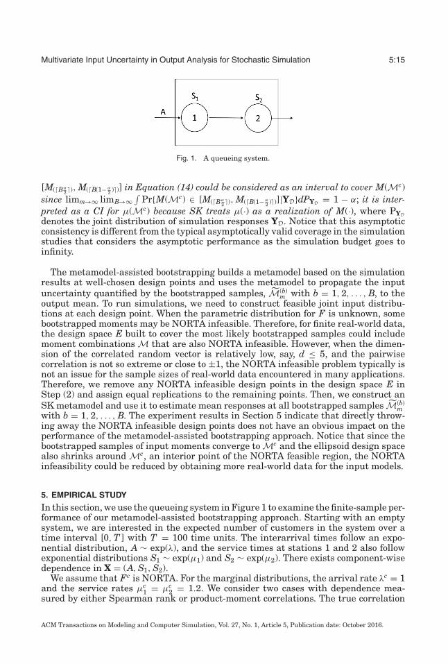
Fig. 1. A queueing system.

[M(�Bα2 �), M(�B(1− α

2 )�)] in Equation (14) could be considered as an interval to cover M(Mc)since limm→∞ limB→∞

∫Pr{M(Mc) ∈ [M(�Bα

2 �), M(�B(1− α2 )�)]|YD}dPYD = 1 − α; it is inter-

preted as a CI for μ(Mc) because SK treats μ(·) as a realization of M(·), where PYDdenotes the joint distribution of simulation responses YD. Notice that this asymptoticconsistency is different from the typical asymptotically valid coverage in the simulationstudies that considers the asymptotic performance as the simulation budget goes toinfinity.

The metamodel-assisted bootstrapping builds a metamodel based on the simulationresults at well-chosen design points and uses the metamodel to propagate the inputuncertainty quantified by the bootstrapped samples, M(b)

m with b = 1, 2, . . . , B, to theoutput mean. To run simulations, we need to construct feasible joint input distribu-tions at each design point. When the parametric distribution for F is unknown, somebootstrapped moments may be NORTA infeasible. Therefore, for finite real-world data,the design space E built to cover the most likely bootstrapped samples could includemoment combinations M that are also NORTA infeasible. However, when the dimen-sion of the correlated random vector is relatively low, say, d ≤ 5, and the pairwisecorrelation is not so extreme or close to ±1, the NORTA infeasible problem typically isnot an issue for the sample sizes of real-world data encountered in many applications.Therefore, we remove any NORTA infeasible design points in the design space E inStep (2) and assign equal replications to the remaining points. Then, we construct anSK metamodel and use it to estimate mean responses at all bootstrapped samples M(b)

mwith b = 1, 2, . . . , B. The experiment results in Section 5 indicate that directly throw-ing away the NORTA infeasible design points does not have an obvious impact on theperformance of the metamodel-assisted bootstrapping approach. Notice that since thebootstrapped samples of input moments converge to Mc and the ellipsoid design spacealso shrinks around Mc, an interior point of the NORTA feasible region, the NORTAinfeasibility could be reduced by obtaining more real-world data for the input models.

5. EMPIRICAL STUDY

In this section, we use the queueing system in Figure 1 to examine the finite-sample per-formance of our metamodel-assisted bootstrapping approach. Starting with an emptysystem, we are interested in the expected number of customers in the system over atime interval [0, T ] with T = 100 time units. The interarrival times follow an expo-nential distribution, A ∼ exp(λ), and the service times at stations 1 and 2 also followexponential distributions S1 ∼ exp(μ1) and S2 ∼ exp(μ2). There exists component-wisedependence in X = (A, S1, S2).

We assume that Fc is NORTA. For the marginal distributions, the arrival rate λc = 1and the service rates μc

1 = μc2 = 1.2. We consider two cases with dependence mea-

sured by either Spearman rank or product-moment correlations. The true correlation


5:16 W. Xie et al.

Table I. Estimated System Mean Response

ρcX = Q ρc = 0 ρc = 0.2 ρc = 0.4 ρc = 0.6 ρc = 0.8

Estimated μ(ϑϑϑc) mean 6.921 6.411 5.913 5.411 4.96Estimated μ(ϑϑϑc) SE 0.01 0.009 0.007 0.0054 0.0036

RcX = Q ρc = 0 ρc = 0.2 ρc = 0.4 ρc = 0.6 ρc = 0.8

Estimated μ(ϑϑϑc) mean 6.93 6.475 5.977 5.472 4.993Estimated μ(ϑϑϑc) SE 0.01 0.009 0.007 0.006 0.004

matrices RcX or ρc

X are

Q ≡( 1 ρc ρc

1 ρc

1

).

For illustration, we set off-diagonal elements in the correlation matrices as a constantvalue. Therefore, the number of parameters characterizing the input model F is d′ =d† + d∗ = 3 + (3 × 2)/2 = 6. Since the true mean response μ(ϑϑϑc) is unknown, we run105 replications to estimate it with results shown in Table I, which records the meanand standard error (SE) of the estimated system response for different values of ρc.Notice that the dependence level quantified by ρc significantly impacts the systemmean response. In this section, we present the empirical results for ρc = 0.4 or 0.8,which are representative of the performance of our metamodel-assisted bootstrappingapproach.

To evaluate metamodel-assisted bootstrapping, we pretend that the input modelparameters (θθθ c, Rc

X) or (θθθ c, ρcX) are unknown and that they are estimated by m i.i.d.

observations from Fc; this represents obtaining “real-world data.” The goal is to builda CI quantifying the impact of both input and simulation estimation error on the systemmean response estimate.

We compare metamodel-assisted bootstrapping to the conditional CI and direct boot-strapping. For the conditional CI, we fit the input distribution to the real-world databy moment matching and allocate the entire computational budget of N replications tosimulating the resulting system. In direct bootstrapping, we run N/B replications ofthe simulation at each bootstrap moment M(b)

m , record the average simulation outputYb = Y (M(b)

m ), and report the percentile CI [Y(�Bα2 �), Y(�B(1− α

2 )�)]. In metamodel-assistedbootstrapping, we evenly assign N replications to K design points, run simulations,build an SK metamodel, and record the percentile CI [M(�Bα

2 �), M(�B(1− α2 )�)] by following

the procedure in Section 4.4.When we construct the stochastic kriging metamodel, we first use an LHD to find

potential design points to evenly cover the ellipsoid design space E. There may existNORTA infeasible design points. For ease of implementation, we throw away thoseNORTA infeasible points and allocate all the computational budget to the remainingdesign points, which is called “Design D1.” This experiment design would not causemetamodel bias under the assumption that the true unknown response surface μ(·) isa realization of a GP. To see if directly removing the NORTA infeasible design pointscould impact the performance of our metamodel-assisted bootstrap approach, we alsomake some modification and obtain “Design D2.” Since Ghosh and Henderson [2002b]indicate that we could always find a close NORTA feasible approximation to a NORTAinfeasible point, we replace NORTA infeasible points with close new design points thatare NORTA feasible. Specifically, we find a close positive semidefinite approximationfor ρZ, denoted by ρZ [Higham 2002], and let ρa

Z ≡ ρZ + δ′Id×d, where Id×d denotes ad× d identity matrix and δ′ is a small positive value. We use δ′ = 10−7 in the empirical



Table II. Results for Nominal 95% CIs When m = 100, 500, 1, 000 When the Dependence IsCharacterized by Spearman Rank Correlations Rc

X = Q

m = 100 ρc = 0.4 ρc = 0.8

N = 103 N = 104 N = 103 N = 104

conditional CI coverage 5.2% 2.7% 7.6% 3.4%CI width (mean) 0.322 0.099 0.158 0.052

CI width (SD) 0.117 0.034 0.043 0.014direct bootstrap coverage 99.4% 96.3% 100% 96.8%

CI width (mean) 14.301 9.515 6.778 4.402CI width (SD) 4.588 3.214 1.908 1.469

metamodel-assisted coverage 93.8% 94.2% 95.8% 95.1%bootstrap CI width (mean) 9.248 8.954 3.978 4.095

CI width (SD) 3.43 3.084 1.307 1.393

m = 500 ρc = 0.4 ρc = 0.8

N = 103 N = 104 N = 103 N = 104

conditional CI coverage 12.3% 4% 15.5% 4.9%CI width (mean) 0.298 0.094 0.151 0.048

CI width (SD) 0.053 0.017 0.019 0.006direct bootstrap coverage 100% 99.1% 100% 99.2%



CI width (SD) 0.795 0.693 0.3 0.246

m = 1000 ρc = 0.4 ρc = 0.8

N = 103 N = 104 N = 103 N = 104





CI width (SD) 0.532 0.345 0.236 0.123

study. Then, we set ρaZ as the correlation matrix for NORTA and generate samples of

X for simulation runs.In direct bootstrapping, for the small percentage of NORTA infeasible bootstrap

resampled moments M(b)m , we first find a close NORTA feasible approximation by fol-

lowing the approach used in Design D2. Then, we use this approximated input modelto drive the simulations and estimate the system performance.

For the input distribution with dependence characterized by either Spearman rankor product-moment correlations, Tables II and III show the statistical performance ofconditional and direct bootstrapping CIs and metamodel-assisted bootstrapping withm = 100, 500, 1,000 real-world observations and computational budget of N = 103, 104

replications. Since the studies by Jones et al. [1998] and Loeppky et al. [2009] rec-ommend that the number of design points should be 10 times the dimension of theproblem for kriging, we set the number of design points K = 60. We ran 1,000 macro-replications of the entire experiment. In each macro-replication, we first generate mmultivariate observations by using NORTA with parameters (θθθ c, Rc

X) or (θθθ c, ρcX). Then,


5:18 W. Xie et al.

Table III. Results for Nominal 95% CIs When m = 100, 500, 1,000 When the DependenceIs Characterized by Product-Moment Correlations ρc

X = Q

ρc = 0.4 ρc = 0.8

m = 100 N = 103 N = 104 N = 103 N = 104

conditional CI coverage 7.7% 2.1% 7.6% 2%CI width (mean) 0.315 0.097 0.155 0.049

CI width (SD) 0.117 0.034 0.045 0.014direct bootstrap coverage 99.1% 97.7% 99.8% 96.2%



(Design D1) CI width (SD) 3.468 3.074 1.372 1.338metamodel-assisted coverage 93.2% 95.6% 95.4% 95.3%

bootstrap CI width (mean) 9.08 8.754 3.841 3.812(Design D2) CI width (SD) 3.466 3.073 1.388 1.335

ρc = 0.4 ρc = 0.8

m = 500 N = 103 N = 104 N = 103 N = 104




metamodel-assisted coverage 94.2% 94.7% 94.6% 95%bootstrap CI width (mean) 3.419 3.386 1.45 1.435

(Design D1) CI width (SD) 0.751 0.671 0.266 0.23metamodel-assisted coverage 94.5% 95% 95.3% 94.9%


ρc = 0.4 ρc = 0.8

m = 1000 N = 103 N = 104 N = 103 N = 104


CI width (SD) 0.035 0.011 0.014 0.004direct bootstrap coverage 100% 99.9% 100% 100%



(Design D1) CI width (SD) 0.449 0.332 0.194 0.125metamodel-assisted coverage 95.5% 94.7% 95.2% 93.9%


for the conditional CI, we run N replications at the estimated parameters (θθθm, RX,m) or(θθθm, ρX,m) and build CIs with nominal 95% coverage of the response mean. For directbootstrapping and metamodel-assisted bootstrapping, we use bootstrapping to generateB = 1,000 sample moments to quantify the input uncertainty. Since μ(·) is unknown,we use the fixed computational budget N to propagate the input uncertainty either viadirect simulation or via the SK metamodel to build percentile CIs with nominal 95%coverage.



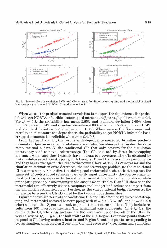
Fig. 2. Scatter plots of conditional CIs and CIs obtained by direct bootstrapping and metamodel-assistedbootstrapping with m = 500, N = 103, and ρc = 0.4, 0.8.

When we use the product-moment correlation to measure the dependence, the proba-bility to get NORTA infeasible bootstrapped moments M(b)

m is negligible when ρc = 0.4.For ρc = 0.8, the probability has mean 3.55% and standard deviation 2.65% whenm = 100, mean 3.14% and standard deviation 4.08% when m = 500, and mean 1.54%and standard deviation 3.29% when m = 1,000. When we use the Spearman rankcorrelation to measure the dependence, the probability to get NORTA infeasible boot-strapped moments is negligible when ρc = 0.4, 0.8.

From Tables II and III, the results with dependence measured by either product-moment or Spearman rank correlations are similar. We observe that under the samecomputational budget N, the conditional CIs that only account for the simulationuncertainty tend to have undercoverage. The CIs obtained by direct bootstrappingare much wider and they typically have obvious overcoverage. The CIs obtained bymetamodel-assisted bootstrapping with Designs D1 and D2 have similar performanceand they have coverage much closer to the nominal level of 95%. As N increases and thesimulation estimation error decreases, the undercoverage problem for the conditionalCI becomes worse. Since direct bootstrap and metamodel-assisted bootstrap use thesame set of bootstrapped samples to quantify input uncertainty, the overcoverage forthe direct bootstrap represents the additional simulation uncertainty introduced whilepropagating the input uncertainty to the output mean. Tables II and III show that themetamodel can effectively use the computational budget and reduce the impact fromthe simulation estimation error. Further, as the computational budget increases, thedifference between the CIs obtained by the two methods diminishes.

Figure 2 shows scatter plots of conditional CIs and CIs obtained by direct bootstrap-ping and metamodel-assisted bootstrapping with m = 500, N = 103, and ρc = 0.4, 0.8when we use either Spearman-rank or product-moment correlations. They include re-sults from 100 macro-replications. The horizontal axis represents (QL + QU )/2, thecenter of the CI, where QL and QU are the lower and upper bounds of the CIs. Thevertical axis is (QU − QL)/2, the half-width of the CIs. Region 1 contains points that cor-respond to CIs having underestimation and Region 3 contains points corresponding tooverestimation, while Region 2 contains CIs that cover μ(Fc); see Kang and Schmeiser


5:20 W. Xie et al.

[1990]. The conclusions obtained for Spearman rank and product-moment correlationsare similar. Since the standard deviation of the system response estimate increaseswith the mean, we observe that all CIs tend to be wider when the center is larger.Conditional CIs have width too short and their centers have large variance. Therefore,they have serious undercoverage. The variance for centers of CIs comes from the impactof input uncertainty. Since metamodel-assisted bootstrapping accounts for both inputand simulation uncertainty, its CI width is large enough to avoid undercoverage. Theproportion of CIs in Region 2 is close to 95%, and CIs outside tend to have underestima-tion based on results from 1,000 macro-replications. The CIs obtained by Designs D1and D2 have similar performance. The width of CIs obtained by the direct bootstrap istoo large; all CIs are located in Region 2 and they have serious overcoverage.

6. CONCLUSIONS

In this paper, we extended the metamodel-assisted bootstrapping framework of Xieet al. [2015] to stochastic simulation with dependent input models. The input modelsare characterized by their marginal distribution parameters and dependence measuredeither by Spearman rank or product-moment correlations, which are estimated fromreal-world data. Metamodel-assisted bootstrapping uses the bootstrap to quantify theestimation error of these joint distributions and propagates it to the output meanby using an equation-based SK metamodel. We proposed a procedure to deliver a CIquantifying the overall uncertainty of the system performance estimate. The asymp-totic consistency of this interval is proved under the assumption that the true meanresponse surface is a realization of a GP. Our metamodel-assisted bootstrap frameworkis applicable to cases when the parametric family of multivariate input distribution isknown or unknown. When the parametric joint input distributions are unknown, weconstruct the joint distributions by using the flexible NORTA representation.

An empirical study using a queueing example demonstrates that for the input dis-tribution with dependence measured by either Spearman rank or product-momentcorrelations, our metamodel-assisted bootstrap approach has good finite-sample per-formance under various quantities of real-world data and simulation budget. When thesimulation budget is tight, compared with the direct bootstrap, the metamodel-assistedbootstrap can make more effective use of the simulation budget.

ELECTRONIC APPENDIX

The electronic appendix for this article can be accessed in the ACM Digital Library.

ACKNOWLEDGMENTS

This research was partially supported by National Science Foundation Grant CMMI-1068473 and GOALIsponsor Simio. The authors thank Cheng Li in the proof of Lemma A.3. Portions of this were previouslypublished in the Proceedings of the 2014 Winter Simulation Conference as Xie et al. [2014b].

REFERENCES

Bruce E. Ankenman, Barry L. Nelson, and Jeremy Staum. 2010. Stochastic kriging for simulation metamod-eling. Operations Research 58 (2010), 371–382.

Eusebio Arenal-Gutierrez, Carlos Matran, and Juan A. Cuesta-Albertos. 1996. Unconditional Glivenko-Gantelli-type theorems and weak laws of large numbers for bootstrap. Statistics & Probability Letters26 (1996), 365–375.

Francois Bachoc. 2013. Cross validation and maximum likelihood estimations of hyper-parameters of Gaus-sian processes with model misspecification. Computational Statistics & Data Analysis 66 (2013), 55–69.

Russell R. Barton. 2007. Presenting a more complete characterization of uncertainty: Can it be done? In Pro-ceedings of the 2007 INFORMS Simulation Society Research Workshop. INFORMS Simulation Society,Fontainebleau.



Russell R. Barton. 2012. Tutorial: Input uncertainty in output analysis. In Proceedings of the 2012 WinterSimulation Conference, C. Laroque, J. Himmelspach, R. Pasupathy, O. Rose, and A. M. Uhrmacher (Eds.).IEEE Computer Society, 67–78.

Russell R. Barton, Barry L. Nelson, and Wei Xie. 2014. Quantifying input uncertainty via simulation confi-dence intervals. Informs Journal on Computing 26 (2014), 74–87.

Russell R. Barton and Lee W. Schruben. 1993. Uniform and bootstrap resampling of input distributions. InProceedings of the 1993 Winter Simulation Conference, G. W. Evans, M. Mollaghasemi, E. C. Russell,and W. E. Biles (Eds.). IEEE Computer Society, 503–508.

Russell R. Barton and Lee W. Schruben. 2001. Resampling methods for input modeling. In Proceedings of the2001 Winter Simulation Conference, B. A. Peters, J. S. Smith, D. J. Medeiros, and M. W. Rohrer (Eds.).IEEE Computer Society, 372–378.

Bahar Biller and Canan G. Corlu. 2011. Accounting for parameter uncertainty in large-scale stochasticsimulations with correlated inputs. Operations Research 59 (2011), 661–673.

Bahar Biller and Soumyadip Ghosh. 2006. Multivariate input processes. In Handbooks in Operations Re-search and Management Science: Simulation, S. Henderson and B. L. Nelson (Eds.). Elsevier, Chapter 5.

Patrick Billingsley. 1995. Probability and Measure. Wiley-Interscience, New York.Marne C. Cario and Barry L. Nelson. 1997. Modeling and Generating Random Vectors with Arbitrary

Marginal Distributions and Correlation Matrix. Technical report. Department of Industrial Engineeringand Management Sciences, Northwestern University.

Xi Chen, Bruce E. Ankenman, and Barry L. Nelson. 2012. The effect of common random numbers onstochastic kriging metamodels. ACM Transactions on Modeling and Computer Simulation 22 (2012),7:1–7:20.

Russell C. H. Cheng and Wayne Holland. 1997. Sensitivity of computer simulation experiments to errors ininput data. Journal of Statistical Computation and Simulation 57 (1997), 219–241.

Robert T. Clemen and Terence Reilly. 1999. Correlations and copulas for decision and risk analysis. Manage-ment Science 45 (1999), 208–224.

Sourav Das, Tata S. Rao, and Georgi N. Boshnakov. 2012. On the Estimation of Parameters of Variograms ofSpatial Stationary Isotropic Random Processes. Research Report No. 2. The University of Manchester.

Soumyadip Ghosh and Shane G. Henderson. 2002a. Chessboard distributions and random vectors withspecified marginals and covariance matrix. Operations Research 50 (2002), 820–834.

Soumyadip Ghosh and Shane G. Henderson. 2002b. Properties of the NORTA method in higher dimensions.In Proceedings of the 2002 Winter Simulation Conference, E. Yucesan, C. H. Chen, J. L. Snowdon, and J.M. Charnes (Eds.). IEEE Computer Society, 263–269.

Peter Hall. 1988. Rate of convergence in bootstrap approximations. The Annals of Probability 16 (1988),1665–1684.

Shane G. Henderson, Belinda A. Chiera, and Roger M. Cooke. 2000. Generating dependent quasi-randomnumbers. In Proceedings of the 2000 Winter Simulation Conference, J. A. Joines, R. R. Barton, K. Kang,and P. A. Fishwick (Eds.). IEEE Computer Society, 527–536.

Nicholas J. Higham. 2002. Computing the nearest correlation matrix – A problem from finance. IMA Journalon Numerical Analysis 22 (2002), 329–343.

Mark E. Johnson. 1987. Multivariate Statistical Simulation. Wiley, New York.Donald R. Jones, Matthias Schonlau, and William J. Welch. 1998. Efficient global optimization of expensive

black-box functions. Journal of Global Optimization 13 (1998), 455–492.Keebom Kang and Bruce Schmeiser. 1990. Graphical methods for evaluation and comparing confidence-

interval procedures. Operations Research 38, 3 (1990), 546–553.Shing T. Li and Joseph L. Hammond. 1975. Generation of pseudorandom numbers with specified univari-

ate distributions and correlation coefficients. IEEE Transactions on Systems, Man, and Cybernetics 5(September 1975), 557–561.

Jason L. Loeppky, Jerome Sacks, and William J. Welch. 2009. Choosing the sample size of a computerexperiment: A practical guide. Technometrics 51 (2009), 366–376.

Tanmoy Mukhopadhyay, Sushanta Chakroborty, Sondipon Adhikari, and Rajib Chowdhury. 2016. Acritical assessment of kriging model variants for high-fidelity uncertainty quantification in dy-namics of composite shells. Archives on Computational Methods in Engineering (2016). Onlineversion.

Bruce W. Schmeiser and Ram Lal. 1982. Bivariate gamma random vectors. Operations Research 30, 2 (1982),355–374.

Jun Shao and Dongsheng Tu. 1995. The Jackknife and Bootstrap. Springer-Verlag.


5:22 W. Xie et al.

Eunhye Song, Barry L. Nelson, and C. Dennis Pegden. 2014. Advanced tutorial: Input uncertainty quantifi-cation. In Proceedings of the 2014 Winter Simulation Conference, A. Tolk, S. Y. Diallo, I. O. Ryzhov, L.Yilmaz, S. Buckley, and J. A. Miller (Eds.). IEEE Computer Society.

A. W. Van Der Vaart. 1998. Asymptotic Statistics. Cambridge University Press, Cambridge, UK.William R. Wade. 2010. An Introduction to Analysis (4th ed.). Prentice Hall.Wei B. Wu and Jan Mielniczuk. 2010. A new look at measuring dependence. In Dependence in Probability

and Statistics, P. Doukhan, G. Lang, D. Surgailis, and G. Teyssiere (Eds.). Springer.Wei Xie, Barry L. Nelson, and Russell R. Barton. 2014a. A Bayesian framework for quantifying uncertainty

in stochastic simulation. Operational Research 62, 6 (2014), 1439–1452.Wei Xie, Barry L. Nelson, and Russell R. Barton. 2014b. Statistical uncertainty analysis for stochastic

simulation with dependent input models. In Proceedings of the 2014 Winter Simulation Conference, A.Tolk, S. Y. Diallo, I. O. Ryzhov, L. Yilmaz, S. Buckley, and J. A. Miller (Eds.). IEEE Computer Society.

Wei Xie, Barry L. Nelson, and Russell R. Barton. 2015. Statistical uncertainty analysis for stochastic simula-tion. (2015). Working Paper, Department of Industrial and Systems Engineering, Rensselaer PolytechnicInstitute, Troy, NY.

Wei Xie, Barry L. Nelson, and Jeremy Staum. 2010. The influence of correlation functions on stochastickriging metamodels. In Proceedings of the 2010 Winter Simulation Conference, B. Johansson, S. Jain, J.Montoya-Torres, J. Hugan, and E. Yucesan (Eds.). IEEE Computer Society, 1067–1078.

Jun Yin, Szu H. Ng, and Kien M. Ng. 2009. A study on the effects of parameter estimation on kriging model’sprediction error in stochastic simulation. In Proceedings of the 2009 Winter Simulation Conference, B.Johansson A. Dunkin M. D. Rossetti, R. R. Hill and R. G. Ingalls (Eds.). IEEE Computer Society, 674–685.

Received October 2014; revised July 2016; accepted August 2016


Documents

Multivariate Input Uncertainty in Output Analysis for ...homepages.rpi.edu/~xiew3/XieBartonNelsonMultivariate_2016.pdfMultivariate Input Uncertainty in Output Analysis for Stochastic