A Model of Homogeneous Input Demand Under Price Uncertaintyweb.stanford.edu/group/fwolak/cgi-bin/sites/default/files/files/... · A Model of Homogeneous Input Demand Under Price Uncertainty

A Model of Homogeneous Input Demand Under Price Uncertainty

By FRANK A. WOLAK AND CHARLES D. KOLSTAD*

This paper examines the empirical validity of a model of homogeneous input demand under price uncertainty in which firms trade off expected input cost against its variability (risk) in selecting the optimal input supplier mix. Using recent work in time-series econometrics, this model is applied to the Japanese steam-coal import market, where five suppliers compete: China, the Soviet Union, South Africa, the United States, and Australia. (JEL L10, L72)

The purpose of this paper is to derive and examine the empirical validity of a model of homogeneous input demand under price uncertainty. The motivation for this investi- gation is the common observation that firms simultaneously purchase a homogeneous factor of production from a variety of suppliers each charging a different price. More- over, there are many instances when the price from one supplier is consistently above that of all other suppliers for an extended period of time yet firms continue to purchase from this supplier. This observation appears to violate the criterion of expected cost minimization for input choice.1 An at-

tempt to explain these anomalies suggests that firms trade off the level of expected input cost against its variability in deciding how to allocate total input demand across available suppliers. By purchasing inputs from a variety of suppliers, the firm is diver- sifying away some of the price risk associated with satisfying demand from the single least-expected-cost supplier.2

Although the marginal rate of substitution (MRS) between risk and cost is not directly observable, we develop a methodology for empirically estimating this magnitude from a time-series of input purchases. This MRS is an estimate of the firm's risk preferences at the expected cost-risk pair selected. If we assume that this MRS between risk and cost is constant across all expected cost-risk pairs, then an input-price risk premium can be calculated. Subject to this assumption, the input-price risk premium is the percentage above the current

* Department of Economics, Stanford University, Stanford, CA 94305, and Department of Economics and Institute for Environmental Studies, University of Illinois, Urbana, IL 61801, respectively. We thank sem- inar participants at Stanford University, the University of California-Berkeley, the University of Texas, the University of Washington, Purdue University, and the Norwegian School of Economics for comments on earlier drafts. Tom MaCurdy, Randy Mariger, Paul Newbold, Roger Noll, and Agnar Sandmo deserve spe- cial mention for their helpful comments. Vivian Hamil- ton expertly prepared the figures. We especially thank an anonymous referee for thoughtful comments and suggestions on the previous version of the paper. His many contributions are too numerous to mention indi- vidually. The final version of this paper was prepared while Wolak was a National Fellow of the Hoover Institution.

IFor the sake of simplicity, assume that the price series are independent and identically distributed draws from a multivariate distribution. The null hypothesis of equal means for the prices becomes less likely the

greater the number of observations that one price series remains above the others. Clearly, if firms are minimizing expected cost, they would purchase all of this input from the least-expected-price supplier. Hence, in this simple case, the nonzero market share of the consistently high-priced supplier is, with high probability, a violation of the expected-cost-minimization criterion of input choice.

2Previous authors (Agnar Sandmo, 1971; Raveendra N. Batra and Aman Ullah, 1974; Roger D. Blair, 1974) have theoretically examined the comparative statistics of firm behavior under input and output price uncertainty.

514

VOL. 81 NO. 3 WOLAKAND KOLSTAD: UNCERTAIN INPUT DEMAND 515

TABLE 1-SUMMARY STATISTICS FOR PRICES AND QUANTITY SHARES

(SAMPLE PERIOD: MAY 1983-MAY 1987)

Mean price ( 103 yen Standard deviation Mean Standard deviation Country k metric ton J of price quantity share of quantity share

China 10.49 2.60 0.087 0.025 Soviet Union 8.95 1.67 0.036 0.015 United States 14.00 3.07 0.119 0.052 South Africa 10.57 2.39 0.213 0.054 Australia 10.54 2.45 0.547 0.087

Data Source: Japan Export and Imports: Commodity by Country.

expected market price a firm would pay for riskless input supply. If the firm's preferences imply a declining MRS between risk and expected cost (the MRS depends on the level of these two magnitudes), then the risk premium we compute is only an upper bound on the percentage above the current expected price the firm would be willing to pay for riskless input supply. Our risk-diversification model of input demand also provides a framework for quantifying the relative risk characteristics of input prices similar to the framework for assessing the relative risk of securities in the capital- asset-pricing model (CAPM). This framework will be discussed later in the paper.

We have chosen the Japanese steam-coal import market for an empirical implementa- tion of the risk-diversification model. This coal is primarily used in Japanese cement- manufacturing and electricity-generation facilities. Although this coal is supplied to a variety of consumers in Japan, the Ministry of International Trade and Industry (MITI) is the centralized decision-maker which co- ordinates all international steam-coal trans- actions and hence is analogous to the firm in our model of input demand. We estimate the risk-diversification model and examine its validity as an explanation for the observed patterns of Japanese steam-coal imports.

The specific puzzle we address is: why do the Japanese not buy the least-expected-cost coal? Three observations about the time- series properties of the vector of yen prices and quantities of steam coal imported from

the five suppliers-China, the Soviet Union, the United States, South Africa, and Aus- tralia-provide evidence against the expected-cost-minimization model of input choice. Table 1 gives the mean price in thousands of yen per metric ton and the mean quantity share, as well as the standard errors for both of these quantities, for these five countries over our sample period.

The first observation is that the price of United States coal is above that of all other suppliers throughout the entire sample period, yet the United States supplies an average of 11.9 percent of all steam coal imported to Japan during this period. The second observation is that the price of steam coal from the Soviet Union is consistently below the price of all other suppliers throughout the sample although it consistently has the smallest share of the Japanese steam-coal import market. These two observations are confirmed by the sample means of the prices given in Table 1. The final puzzle is that South Africa and Australia have approximately the same mean price over the sample, although for all observations over this same period the share of Japanese steam-coal imports from Australia is consistently more than double that from South Africa. We find that the risk-diversification model and the apparent risk characteristics that it implies for each supplier provide an economically plausible explanation of the operation of the Japanese steam-coal import market.

The remainder of the paper proceeds as follows. The next section introduces nota-

516 THE AMERICAN ECONOMIC REVIEW JUNE 1991

tion and then derives the risk-diversification model of input demand. Section II discusses the econometric framework underlying the estimation of this model. This section treats the specification of a stochastic process describing the behavior of the vector of input prices over time and also describes the form and sources of other uncertainty in the model. Section III provides a brief overview of the Japanese steam-coal import market, to match up the theoretical model of Sec- tion I with the actual workings of this market. Section IV describes the application of this framework to the Japanese steam-coal import market. It presents several formal and informal tests of our structural model embodying the risk-diversification hypothesis. In Section V, we present the general implications of modeling input demand under uncertainty within this risk-diversification framework. For example, we are able to calculate the risk premium described earlier and a measure of market-specific risk associated with each of the supply-price processes. We can also derive a relationship between these measures of market-specific risk and the optimal expected supply price for each supplier. We then examine the validity of these implications of our structural model within the context of the Japanese steam-coal market. The paper closes with a short discussion of the policy implications of the empirical results and suggestions for future applications of this framework.

I. A Risk-Diversification Model of Firm Input Demand

Consider a firm using a set of inputs to produce one or more outputs. All inputs to production but one are termed "nonrisky" in that their price is nonstochastic. Output prices are also nonstochastic. The price of one of the inputs (the "risky" input) is uncertain. Supplies of that input must be con- tracted for ex ante before the price uncertainty is resolved. If the firm is risk-averse, it may increase its utility by substituting away from the risky input or by utilizing a variety of suppliers in an effort to reduce risk through diversification.

We begin by defining notation:

Pit: price of risky input from supplier i in period t (i = 1,..., n);

q,t: quantity of risky input demanded from supplier i in period t (i = 1, .. ., n);

Pt: n-dimensional vector of risky-input prices in period t;

qt: n-dimensional vector of risky-input quantities demanded in period t;

rt: vector of prices of nonrisky inputs in period t;

st: vector of quantities of nonrisky inputs in period t;

st: vector of deterministic output prices in period t;

yt: vector of output quantities in period t; It: information set available to firm at time

t, containing p, (s < t - 1); ,.Lt: E(ptIIt), conditional expectation of pt; 5:t: E{(pt - Lt)(pt -Ft)'IIt), conditional

variance of pt; t: n-dimensional vector of l's;

Qt: tl'qt, total demand for risky input in period t;

wt: qt/Qt, n-dimensional vector of risky- input quantity shares.

The firm is governed by the implicit production relation f(yt, st, Qt) = 0. Rather than maximize profits, because it is risk- averse, in each period the firm maximizes the expected utility of profits given the vectors of nonstochastic input and output prices and the information set It. We make the simplifying assumption that the firm's expected utility can be written as a function of the conditional expectation of profits, E(HtlIt), and the conditional variance of profits, V(HtlIt), where

= l' rYt -pqt -rt'st

is the firm's profit in period t. This assumption about firm preferences is similar to that made for investor preferences in the CAPM. As in the CAPM, this assumption is equivalent to either the firm having a utility function that is quadratic in profits or the random input prices pt having a multivariate Gaussian distribution. Thus, the firm's prob-


lem is, at every time period,

( ) max U [E( 7r/tyt - pfqt - rtstllt ), (1) max t qI,SI'Yt

V(,'yt -plqt - rtstlit)]

U [.r;yt -r'st - E(pfqtlItI)

V(pIqtJIJ ]

subject to

f(yt.st,Qt) =? I~ qt = Qt~ qt, st, yt > ?-

This optimization problem is equivalent to the two-stage process whereby first an optimal portfolio of suppliers is chosen to yield a given Qt. Then, in the second stage, the proper balance is struck among outputs (yt), nonrisky inputs (st), and the total amount of the risky input (Q)t. The portfolio of qt for a given Qt, and F (described below) is the solution to

(2) max U [ F - E(p q t [It), V(plqt I1)]

subject to Lqt =Qt, qt2O.

Substituting this vector of optimal supplier quantities back into the objective function yields the optimal-value function U *(F, Q I I t), where F is net revenue from nonrisky inputs and outputs. Thus, U * de- fines the highest level of utility obtainable for a given F and Qt; the optimal q* (which is a function of F and Qt) has been substi- tuted in for qt. The second-stage optimization problem uses this optimal-value function to determine the utility-maximizing total quantity of the risky input (Qt), nonrisky inputs (st), and outputs (yt) as follows:

(3) max U*( t yt-rist,QtIIt) Yt, St, Qt

subject to

f(Yt ISt 5Qt) = ? Qt,st,yt > ?.

Solving (3) with U * defined by (2) is equivalent to solving (1).

Because we are only interested in the choice of the portfolio of suppliers of the risky input, we will focus on (2). Ignoring the possible negativity of any elements of qt, the Lagrangian for (2) is

(4) L = U(F F- Rqt,q 't,tqt)

+ -q(Qt - qt)

where -q is the Lagrange multiplier on the constraint that the sum of purchases from all of the suppliers equals Qt. The first-order conditions from (4) are

dL (5) - = - U1li't + 2U2q' It - -qC = 0

where U, is the derivative of U with respect to its ith argument. Equation (5) can be solved for the scalar i7 using the constraint LIqt = Qt

2U2Qt - U1LYTE1t.Lt (6) 71=t-1

Substituting (6) back into (5) and rearrang- ing gives the following expression for the optimal vector of risky input shares:

(7)

[AtQt + L 11-1 I wt '1. (t1L

- 1

where At = - 2U2/ U1. Dividing At by 2 gives the producer's marginal rate of substitution between expected costs and risk. It is, of course, a function of It. Qt, and F. However, Qt and F, and thus At, are the result of solving (3). Rather than solve (3) explicitly, we make an assumption about the functional form of At. Several specifications for At are possible. The first is simply At = A for all t. Another, which is the specification we adopt, is that At = A/Qt (i.e., AtQt is a constant). This specification for At has the attractive feature that it makes the optimal input share (7) invariant to Qt. Thus, for fixed pt and t, if there is a secular rise in


the level of productive activity in the firm, supplier shares remain constant. This expression for At simplifies (7) to

(8)

[A + L'Xt1-.L i A+tt t> 1I Y

wtO = (I t I) A

For notational ease in what follows we write (8) as

(9) wto = St(Rt It, A).

Defining I = 1/A, we can rewrite (8) as

(10)

?= + (t S Ft) -1) (1 )

Equation (10) gives the optimal-supplier- share vector as a function of 4, the relative weight attached to expected cost in the firm's optimal-input-choice problem, whereas (8) gives the same optimal supplier share as a function of A, the relative weight attached to the conditional variance of input cost. Equation (10) will be used later when we examine the validity of our structural model of the risk-diversification hypothesis.

Given values for wt and t, and knowing its value of A, or equivalently 4, the firm can compute the optimal period-t input- supplier mix from equation (8). We assume that the firm knows or behaves as if it knows the parameters of the stochastic process determining the time path of the vector of input prices so that it can compute wt and Yt for all t. Unfortunately, in order for us to implement this model and determine its empirical validity, we must estimate the parameters of this stochastic process. Therefore, we now turn to the econometrics of the risk-diversification model of input demand.

II. The Econometrics of the Risk-Diversification Model

of Input Demand

In this section, we present our methodology for implementing the risk-diversification

model of input demand. There are two independent sources of uncertainty in this model. The first, what we call estimation error, arises from the estimation of w, and S,, the conditional mean and covariance matrix of the vector-valued price process. The second, what we refer to as optimization error, is included to account for any unobservable time-specific random shocks which may cause the first-order conditions (5) not to hold exactly each period.

This optimization error has the implication that we require the first-order conditions to hold only in expectation. Opera- tionally, this means that (9) becomes

(11) wt =St( lt S t hA) + ?t-Wtt + Et

where ,t E Rn is H/(0, Q). Thus, the observed input-share vector (wt) equals the optimal input-share vector (wto) plus white noise. The restriction that L'Wt = 1 implies that L'Et = 0 and L'ft = 0. We introduce this optimization error as a way to take into account the fact that there may be unobservable (to the econometrician) variables that affect the supplier shares actually selected which are not included in our model of input demand. Hence, despite requiring the total input supply to be deterministic, the model does allow random variation in quantities across suppliers from the utility- maximizing levels determined from our risk-diversification model.

Because our price series appear to be stationary in first-differences yet their levels roughly move together (there exists a stationary linear combination of the prices), our methodology for modeling the estimation error in wt and It involves fitting an error-correction model for each price series:

(12) Apit = C +yizit1 + 3Apit-1 + it

(i=1, ...,n; t-=1, ...,~T)

where Apit = Pit - Pit- 1. To take into account the fact that, on average, the levels of these prices move together we include zl,t which is an estimate of the stationary linear combination of all of the prices. Following


Robert F. Engle and Clive W. J. Granger (1987) and James H. Stock (1987), we compute zi, as the residual from the regression of pi, on all other prices and a constant. Hence, Zit has a sample mean of zero. As shown in Stock (1987), because the parameters of the cointegrating regression converge to their true values at rate T, rather than the usual T, the zit may be effectively treated as the observed zt in the estimation of the parameters of (12) and the computa- tion of their T -asymptotic distribution. We assume that tt = (;lt' 62t'... * *n), is distributed as a -IV(O,) random vector. This distributional assumption for tt and the model (12) for pi (i = 1, ... n) implies that the conditional variance of It equals a constant S for all t.

Besides embodying the cointegration property of pt, this model for each price series is consistent with the following logic. The constant term cl takes into account the possibility that Apit may have a nonzero mean. By including this constant term, we are effectively allowing pit to have a nonzero mean in its stochastic trend. The term in zit-, the error correction term, takes into account the fact that the amount z1t-1 differs from its steady-state value will affect period t's price change for this supplier. We would expect y, to be negative because, if z-1 is positive (recall how zl is estimated), this period's Apit should be lower than its mean to reflect a correction toward the steady state. The third term in Apt_1t represents the impact of last period's price change on this period's price change.

The final model estimated for each price series should be such that the null hypothesis that it- E(pit It)- pt is white noise cannot be rejected. Additional terms in ApJ, (j = 1, ... , n; s < t - 1) should be added to the model until this is the case. Clearly, a shortcoming of our approach is that there may be other variables besides lagged values of pt that help to estimate Ft. Never- theless, in this paper we assume that It contains only lagged values of pt.

Let F, denote all of the coefficients enter- ing into (12) for Apit. Let bit(rit,I) denote the conditional mean function for the ith price process. In this shorthand notation we

can rewrite (12) as

(13) p1t =1 it(rl,1t)+ (it (i = 1.,n).

If we stack all of the ri into a single vector r then we can write (13) in vector notation as:

(14) Pt = Rt(r,it) + tt

Once we fit a univariate model to each price series such that the null hypothesis that each (It series is white noise cannot be rejected, we can construct a consistent estimate of I as follows:

T

Tt = I

where t (1t' 2t,._Ignt)' and (l, is the ordinary least-squares (OLS) estimate of (it. This completes the first step of our two-step procedure to obtain consistent estimates of 52 and r. In summary, the equation-by- equation OLS estimates of the F, in (13) yield a consistent estimate of r, and because i is based on this estimate of r, it is also consistent. The next step of this procedure conditions on these estimates of r and I and computes [from (11)] estimates of A and Q by maximum likelihood (ML). This two-step process yields 4T-consistent estimates of r, 1, A, and fQ which can be used as starting values in a full-model ML estimation procedure.

Combining the model determining wt in (11) with that determining pt in (13) yields the following nonlinear ML model:

( )[t ][St(Lt( r, It,) >A) ][et

where E(4t El) = 0, because the estimation error is assumed to be independent of the optimization error.


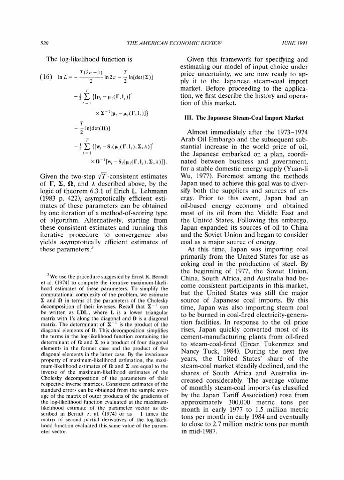
The log-likelihood function is

T(2n-1) T (16) lnL=- -2 1n21r--Tn[det(Y)]

T

t= E {[Pt- pt(F,It)}

X x-1[pt - pt(rjIt)]}

T - - ln[det(Q)]

2 T

-E [wt - st(tLft( r,jIt), x, A )] t1

x Q- l[wt- st(,ut(r, It), 1, A)]).

Given the two-step T -consistent estimates of r, 1, fQ, and A described above, by the logic of theorem 6.3.1 of Erich L. Lehmann (1983 p. 422), asymptotically efficient estimates of these parameters can be obtained by one iteration of a method-of-scoring type of algorithm. Alternatively, starting from these consistent estimates and running this iterative procedure to convergence also yields asymptotically efficient estimates of these parameters.3

Given this framework for specifying and estimating our model of input choice under price uncertainty, we are now ready to ap- ply it to the Japanese steam-coal import market. Before proceeding to the application, we first describe the history and operation of this market.

III. The Japanese Steam-Coal Import Market

Almost immediately after the 1973-1974 Arab Oil Embargo and the subsequent substantial increase in the world price of oil, the Japanese embarked on a plan, coordi- nated between business and government, for a stable domestic energy supply (Yuan-li Wu, 1977). Foremost among the methods Japan used to achieve this goal was to diver- sify both the suppliers and sources of energy. Prior to this event, Japan had an oil-based energy economy and obtained most of its oil from the Middle East and the United States. Following this embargo, Japan expanded its sources of oil to China and the Soviet Union and began to consider coal as a major source of energy.

At this time, Japan was importing coal primarily from the United States for use as coking coal in the production of steel. By the beginning of 1977, the Soviet Union, China, South Africa, and Australia had become consistent participants in this market, but the United States was still the major source of Japanese coal imports. By this time, Japan was also importing steam coal to be burned in coal-fired electricity-generation facilities. In response to the oil price rises, Japan quickly converted most of its cement-manufacturing plants from oil-fired to steam-coal-fired (Ercan Tukenmez and Nancy Tuck, 1984). During the next five years, the United States' share of the steam-coal market steadily declined, and the shares of South Africa and Australia in- creased considerably. The average volume of monthly steam-coal imports (as classified by the Japan Tariff Association) rose from approximately 300,000 metric tons per month in early 1977 to 1.5 million metric tons per month in early 1984 and eventually to close to 2.7 million metric tons per month in mid-1987.

3We use the procedure suggested by Ernst R. Berndt et al. (1974) to compute the iterative maximum-likelihood estimates of these parameters. To simplify the computational complexity of the problem, we estimate Y and Q in terms of the parameters of the Cholesky decomposition of their inverses. Recall that I` can be written as LDL', where L is a lower triangular matrix with l's along the diagonal and D is a diagonal matrix. The determinant of I-1 is the product of the diagonal elements of D. This decomposition simplifies the terms in the log-likelihood function containing the determinant of Q and I to a product of four diagonal elements in the former case and the product of five diagonal elements in the latter case. By the invariance property of maximum-likelihood estimation, the maximum-likelihood estimates of U and I are equal to the inverse of the maximum-likelihood estimates of the Cholesky decomposition of the parameters of their respective inverse matrices. Consistent estimates of the standard errors can be obtained from the sample average of the matrix of outer products of the gradients of the log-likelihood function evaluated at the maximum- likelihood estimate of the parameter vector as described in Berndt et al. (1974) or as - 1 times the matrix of second partial derivatives of the log-likelihood function evaluated this same value of the parameter vector.


This steam coal is imported through ne- gotiations with Japanese trading companies in conjunction with MITI for delivery to the steam-coal-using facilities. Prices for coal are negotiated in terms of the currency of the country of origin of the coal, although sometimes in dollars. Hence, some of the price risk borne by Japanese consumers is due to foreign-exchange-rate risk. An additional source of price uncertainty to Japan arises from what are called demurrage costs. These costs are incurred when a ship pick- ing up or delivering coal is unable to load or unload its cargo immediately upon arrival at port. These queuing costs at port are usu- ally directly added to the delivered price of coal. In periods when loading or unloading facilities are operating at capacity, these charges can amount to a significant portion (approximately 10 percent) of the delivered price of coal (United States Department of Energy, 1981 p. 7).

Coal is purchased using three mecha- nisms: joint venture between buyer and supplier, long-term contract, and short-term supply agreement (this category includes spot-market purchases). In contrast to met- allurgical coal, which is a highly specialized input to the production of steel and as a consequence is, for the most part, delivered on long-term contracts, the relatively simple uses of steam coal and the increasing flexibility of boilers to burn different types of coal make short-term supply agreements (less than one year) and spot-market purchases viable. The Japanese make substantial spot-market purchases from South Africa, the United States, and Australia, while spot purchases play a lesser role in the imports from China and the Soviet Union. As stated in a recent United States Department of Energy report, "At present, South Africa steam-coal exports to Asia are largely spot sales" (Tukenmez and Tuck, 1984 p. xxi).

Most long-term contracts and joint ventures allow for some flexibility in the prices charged for coal delivered on a given contract depending on current market conditions at the time of delivery, so that some of the price risk is due to the conditions in the spot market at the delivery date. Also, in

the case of long-term contracts and joint ventures, the Japanese trading companies often renegotiate the prices charged under these agreements if current market conditions favor their doing so. For example, when there is a downturn in the world coal market many of these contracts are renego- tiated. This potential for renegotiation of long-term supply agreements based on current market conditions is another source of price uncertainty.

There is an abundance of anecdotal evidence for the validity of the risk-diversification model of input choice for the Japanese steam-coal import market. Various editions of the MITI Handbook published by Japan Trade and Industry Publicity, state that the two major policy goals for MITI in the area of energy and natural resources are: 1) a stable supply of energy resources and 2) stable prices of energy resources. One of the stated goals of the Coal Mining Depart- ment of MITI is "to smooth the importation of coal" (MITI Handbook 1979/1980 p. 82). Japan's desire for a stable, secure energy supply is well documented in Wu (1977), a study of Japan's response to the Arab Oil Embargo of 1973/1974. In addition, a U.S. Department of Energy study of coal trade in the Asian market states, "... in seeking diversification and security Japan seems willing to pay a premium to access stable coal supplies from the more expensive ex- porters, such as the United States..." (Tukenmez and Tuck, 1984 p. 3). This ca- sual evidence coupled with the three puzzles concerning the time-series properties of the prices and quantities of imports of steam coal to Japan stated in the Introduction makes for a challenging application of our risk-diversification model of input choice that is also of substantial policy interest.

IV. Application to the Japanese Steam-Coal Import Market

Time-series of prices and quantities of steam coal4 imported into Japan from

4Steam coal is classified by the Japan Tariff Associa- tion as high- and low-ash coal other than coking coal.


China, the Soviet Union, the United States, South Africa, and Australia are available on a monthly basis from Japan Exports and Imports: Commodity by Country, compiled by the Japan Tariff Association. All prices are in units of thousands of yen per metric ton. The quantity units are metric tons. The Appendix describes the construction of these magnitudes from the raw data. Note that the input-choice problem is invariant to the absolute price level. The normalization of prices will only affect the magnitude of A. To make shares and prices of approximately the same magnitude in the estimation procedure, prices were normalized so that the sum of the sample means of all of the prices of coal is equal to 1.

The sample period from March 1983 to May 1987 was selected because the struc- ture of the Japanese steam-coal import market seems stable over this period. Con- firmation of this point is that, despite a growing total quantity of steam coal imported, the share of the market served by each supplier shows no statistically significant serial correlation or trend over this period. This empirical observation provides further support for our selection of a form for At that makes the optimal supplier shares independent of Qt because, as mentioned in Section III, Q, nearly doubled over our sample period.

The first step of the estimation procedure is to test for cointegration among the five price processes over the sample. As discussed in Engle and Granger (1987), the presence of cointegration is necessary for

the validity of the error-correction model of the price processes given in (12). To confirm that each of the univariate price processes is integrated of order one, we performed David A. Dickey and Wayne A. Fuller's (1979) unit-root tests on the levels and first differences of each series. The models run for each test are

(17) Api,=a+ 1p,t_1+82APit- +eit

for the test for a unit root in the levels and

(18) Ypit= a + Pit-1+ 32Ap1t1+ dit

for the test for a unit root in the first differences. In both cases, the null hypothesis is that 81 = 0, or more precisely, the backshift operator polynomial of the AR portion of the ARIMA representation of xt (xt represents either the raw or first-differenced price series) has the following fac- torization: O(B) = (1 - B)O*(B), where all of the roots of + *(z) = 0 are greater than 1 in modulus. The results of these tests are given in Table 2. For all of the tests in terms of the levels of the price series, there is little evidence against the null hypothesis of a unit root, indicating that nonstationarity of the price series in levels cannot be rejected. In contrast, the null hypothesis of a unit root in the first-differenced series is decisively rejected for all of the series at the 0.01 level of significance, providing strong evidence for the stationarity of the first- differenced series. The critical value for the test is from table 8.5.2 of Fuller (1976 p. 373). For the present case, an assumption implicit in the Dickey-Fuller test-that the true value of a is 0 in (17) and (18)-may not be valid given the substantial decline in prices over the sample period. For this reason, we also report Kenneth D. West's (1988) corrected t statistic on ,1 in (17) and (18). This statistic is asymptotically normal under the assumption that a in these two equations is nonzero. Computing West's t statistic amounts to correcting the usual OLS t statistic for the fact that the OLS estimate of the variance of the error term

Although, strictly speaking, steam coal differs across countries, it is primarily, if not exclusively, valued for its heat content. Consequently, only coal with the highest heat content is exported. Although the heat content of each shipment of coal to Japan during the sample period was not available, the heat content of coal for a representative sample of coal contracts from each of the supplier countries considered in this paper was available (TEX Report, 1986). For this representative sample, the mean heat content per ton of coal delivered was not significantly different across the supplier countries considered here. This provides support for our treatment of steam coal from various countries as a homogeneous product.


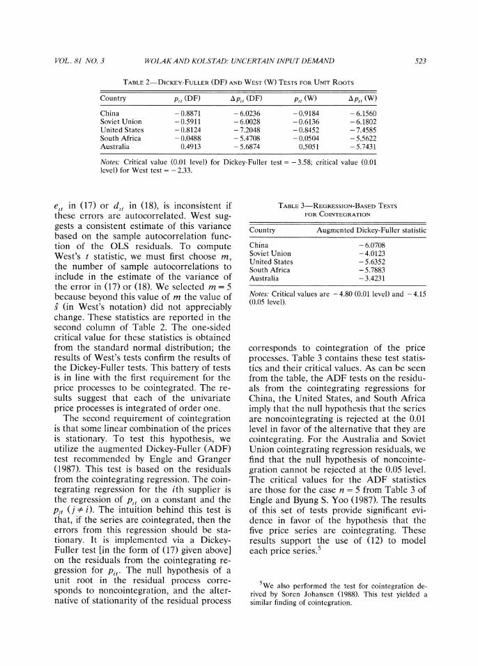
TABLE 2-DICKEY-FULLER (DF) AND WEST (W) TESTS FOR UNIT ROOTS

Country p, (DF) Ap, (DF) p, (W) Ap, (W)

China - 0.8871 - 6.0236 -0.9184 - 6.1560 Soviet Union -0.5911 - 6.0028 -0.6136 - 6.1802 United States - 0.8124 - 7.2048 - 0.8452 - 7.4585 South Africa - 0.0488 - 5.4708 - 0.0504 - 5.5622 Australia 0.4913 -5.6874 0.5051 -5.7431

Notes: Critical value (0.01 level) for Dickey-Fuller test =-3.58; critical value (0.01 level) for West test = - 2.33.

elt in (17) or dit in (18), is inconsistent if these errors are autocorrelated. West suggests a consistent estimate of this variance based on the sample autocorrelation function of the OLS residuals. To compute West's t statistic, we must first choose m, the number of sample autocorrelations to include in the estimate of the variance of the error in (17) or (18). We selected m = 5 because beyond this value of m the value of s (in West's notation) did not appreciably change. These statistics are reported in the second column of Table 2. The one-sided critical value for these statistics is obtained from the standard normal distribution; the results of West's tests confirm the results of the Dickey-Fuller tests. This battery of tests is in line with the first requirement for the price processes to be cointegrated. The results suggest that each of the univariate price processes is integrated of order one.

The second requirement of cointegration is that some linear combination of the prices is stationary. To test this hypothesis, we utilize the augmented Dickey-Fuller (ADF) test recommended by Engle and Granger (1987). This test is based on the residuals from the cointegrating regression. The cointegrating regression for the ith supplier is the regression of pt on a constant and the Pjt (j 0 i). The intuition behind this test is that, if the series are cointegrated, then the errors from this regression should be stationary. It is implemented via a Dickey- Fuller test [in the form of (17) given above] on the residuals from the cointegrating regression for Pit. The null hypothesis of a unit root in the residual process corresponds to noncointegration, and the alternative of stationarity of the residual process

TABLE 3-REGRESSION-BASED TESTS FOR COINTEGRATION

Country Augmented Dickey-Fuller statistic

China - 6.0708 Soviet Union - 4.0123 United States - 5.6352 South Africa - 5.7883 Australia - 3.4231

Notes: Critical values are - 4.80 (0.01 level) and - 4.15 (0.05 level).

corresponds to cointegration of the price processes. Table 3 contains these test statistics and their critical values. As can be seen from the table, the ADF tests on the residuals from the cointegrating regressions for China, the United States, and South Africa imply that the null hypothesis that the series are noncointegrating is rejected at the 0.01 level in favor of the alternative that they are cointegrating. For the Australia and Soviet Union cointegrating regression residuals, we find that the null hypothesis of noncointegration cannot be rejected at the 0.05 level. The critical values for the ADF statistics are those for the case n = 5 from Table 3 of Engle and Byung S. Yoo (1987). The results of this set of tests provide significant evidence in favor of the hypothesis that the five price series are cointegrating. These results support the use of (12) to model each price series.5

5We also performed the test for cointegration derived by Soren Johansen (1988). This test yielded a similar finding of cointegration.


TABLE 4-FIRST-RoUND ESTIMATES OF PRICE PROCESSES

Parameter estimates Specification test statistics

Country c, Y, /31 AR(1) errors ARCH(2) errors

China - 0.0022516 - 0.71658 0.34724 - 0.520287 0.01627 (0.0012798) (0.16424) (0.11850)

Soviet Union - 0.0026191 - 0.74900 - 0.14908 0.137535 2.4991 (0.0015359) (0.18776) (0.13111)

United States - 0.0035828 - 1.16960 - 0.04572 - 0.821971 1.9785 (0.0019120) (0.24895) (0.14853)

South Africa - 0.0028731 - 0.68449 0.104030 - 0.638958 4.4891 (0.0012169) (0.25212) (0.16425)

Australia - 0.0032582 - 0.12764 - 0.34435 0.617483 1.9756 (0.0010532) (0.12171) (0.14205)

Note: Ordinary least-squares standard-error estimates are in parentheses below the coefficient estimates.

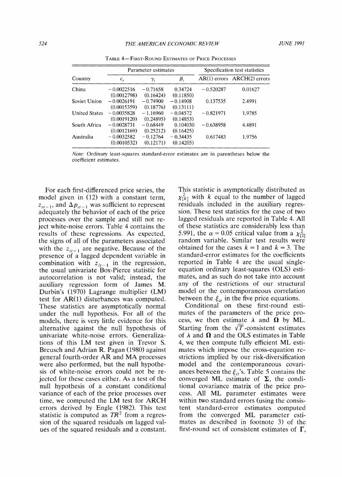
For each first-differenced price series, the model given in (12) with a constant term, zit-1, and Aplt-l was sufficient to represent adequately the behavior of each of the price processes over the sample and still not re- ject white-noise errors. Table 4 contains the results of these regressions. As expected, the signs of all of the parameters associated with the zit-1 are negative. Because of the presence of a lagged dependent variable in combination with zit-1 in the regression, the usual univariate Box-Pierce statistic for autocorrelation is not valid; instead, the auxiliary regression form of James M. Durbin's (1970) Lagrange multiplier (LM) test for AR(1) disturbances was computed. These statistics are asymptotically normal under the null hypothesis. For all of the models, there is very little evidence for this alternative against the null hypothesis of univariate white-noise errors. Generaliza- tions of this LM test given in Trevor S. Breusch and Adrian R. Pagan (1980) against general fourth-order AR and MA processes were also performed, but the null hypothesis of white-noise errors could not be rejected for these cases either. As a test of the null hypothesis of a constant conditional variance of each of the price processes over time, we computed the LM test for ARCH errors derived by Engle (1982). This test statistic is computed as TR2 from a regression of the squared residuals on lagged values of the squared residuals and a constant.

This statistic is asymptotically distributed as X[k] with k equal to the number of lagged residuals included in the auxiliary regression. These test statistics for the case of two lagged residuals are reported in Table 4. All of these statistics are considerably less than 5.991, the a = 0.05 critical value from a X[2] random variable. Similar test results were obtained for the cases k = 1 and k = 3. The standard-error estimates for the coefficients reported in Table 4 are the usual single- equation ordinary least-squares (OLS) estimates, and as such do not take into account any of the restrictions of our structural model or the contemporaneous correlation between the (it in the five price equations.

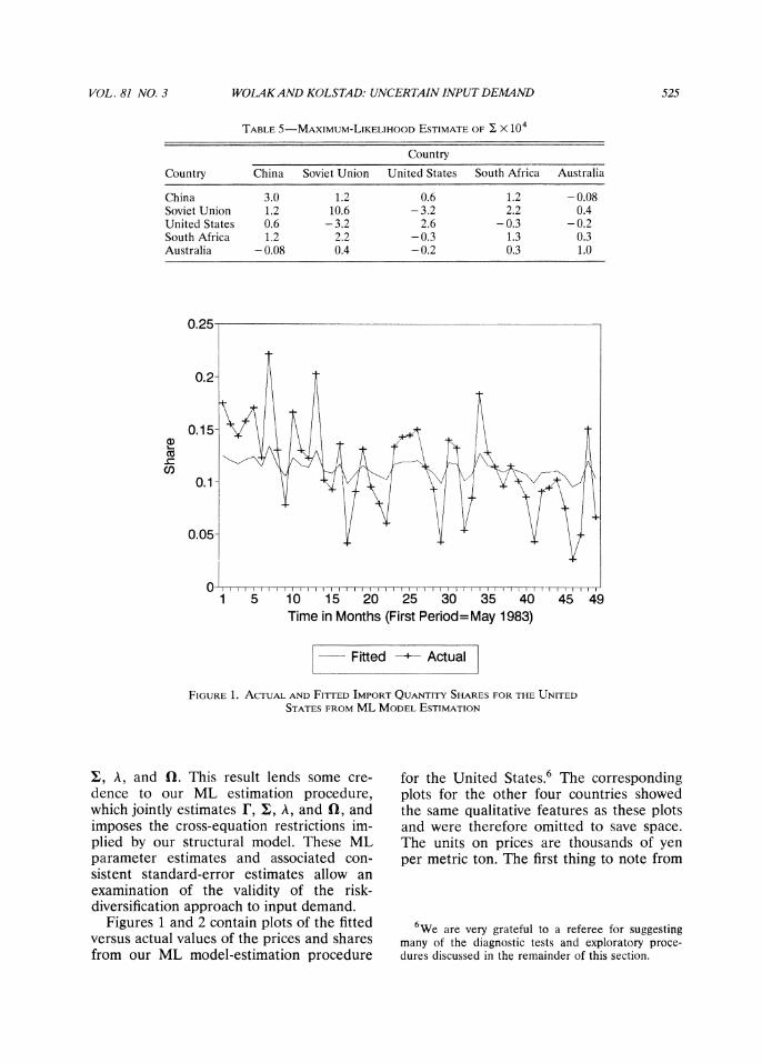
Conditional on these first-round estimates of the parameters of the price process, we then estimate A and Q by ML. Starting from the VT-consistent estimates of A and Q and the OLS estimates in Table 4, we then compute fully efficient ML estimates which impose the cross-equation restrictions implied by our risk-diversification model and the contemporaneous covariances between the nj,'s. Table 5 contains the converged ML estimate of X, the conditional covariance matrix of the price process. All ML parameter estimates were within two standard errors (using the consistent standard-error estimates computed from the converged ML parameter estimates as described in footnote 3) of the first-round set of consistent estimates of F,


TABLE 5-MAXIMUM-LIKELIHOOD ESTIMATE OF E X 104

Country

Country China Soviet Union United States South Africa Australia

China 3.0 1.2 0.6 1.2 -0.08 Soviet Union 1.2 10.6 -3.2 2.2 0.4 United States 0.6 -3.2 2.6 -0.3 -0.2 South Africa 1.2 2.2 -0.3 1.3 0.3 Australia -0.08 0.4 -0.2 0.3 1.0

0.25.

0.2-

0.15X CD cu

co 0.1

0.05-

0 ii I III I I I 1--' 1 I I I i I

1 5 10 15 20 25 30 35 40 45 49 Time in Months (First Period=May 1983)

0 Fitted -+ Actual

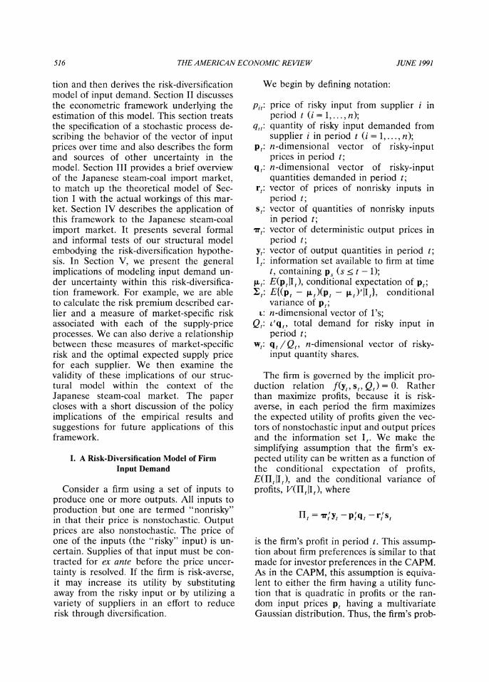
FIGURE 1. ACTUAL AND FITrED IMPORT QUANTITY SHARES FOR THE UNITED

STATES FROM ML MODEL ESTIMATION

X, A, and Q. This result lends some cre- dence to our ML estimation procedure, which jointly estimates r, 1, A, and Q, and imposes the cross-equation restrictions implied by our structural model. These ML parameter estimates and associated consistent standard-error estimates allow an examination of the validity of the risk- diversification approach to input demand.

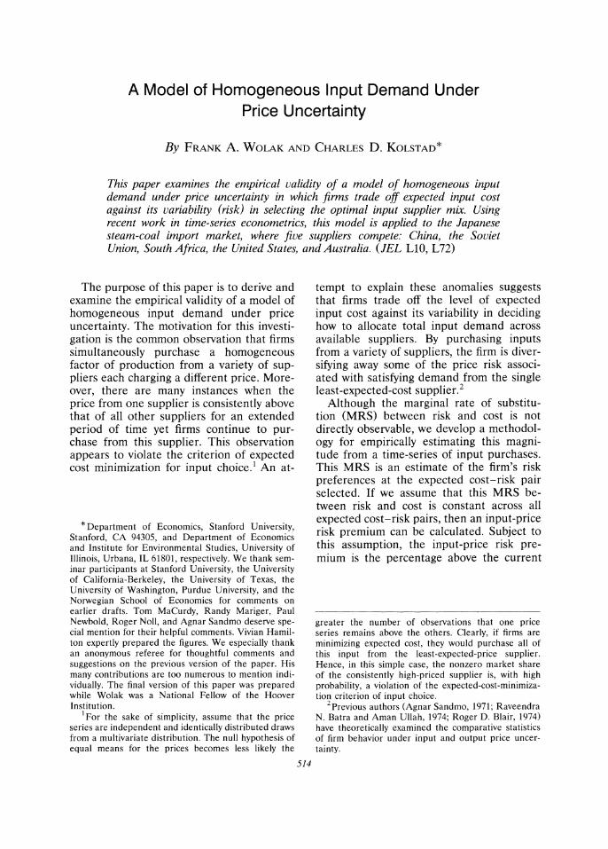
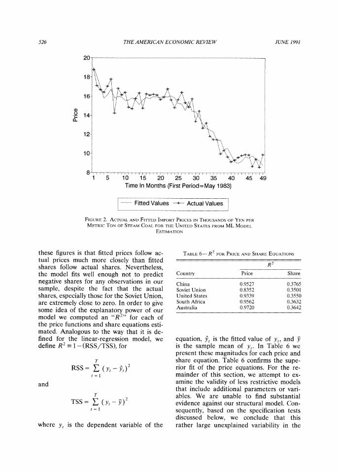
Figures 1 and 2 contain plots of the fitted versus actual values of the prices and shares from our ML model-estimation procedure

for the United States.6 The corresponding plots for the other four countries showed the same qualitative features as these plots and were therefore omitted to save space. The units on prices are thousands of yen per metric ton. The first thing to note from

6We are very grateful to a referee for suggesting many of the diagnostic tests and exploratory proce- dures discussed in the remainder of this section.


20

12-

10

8 1 5 10 15 20 25 30 35 40 45 49

Time In Months (First Period=May 1983)

; Fitted Values + Actual Values

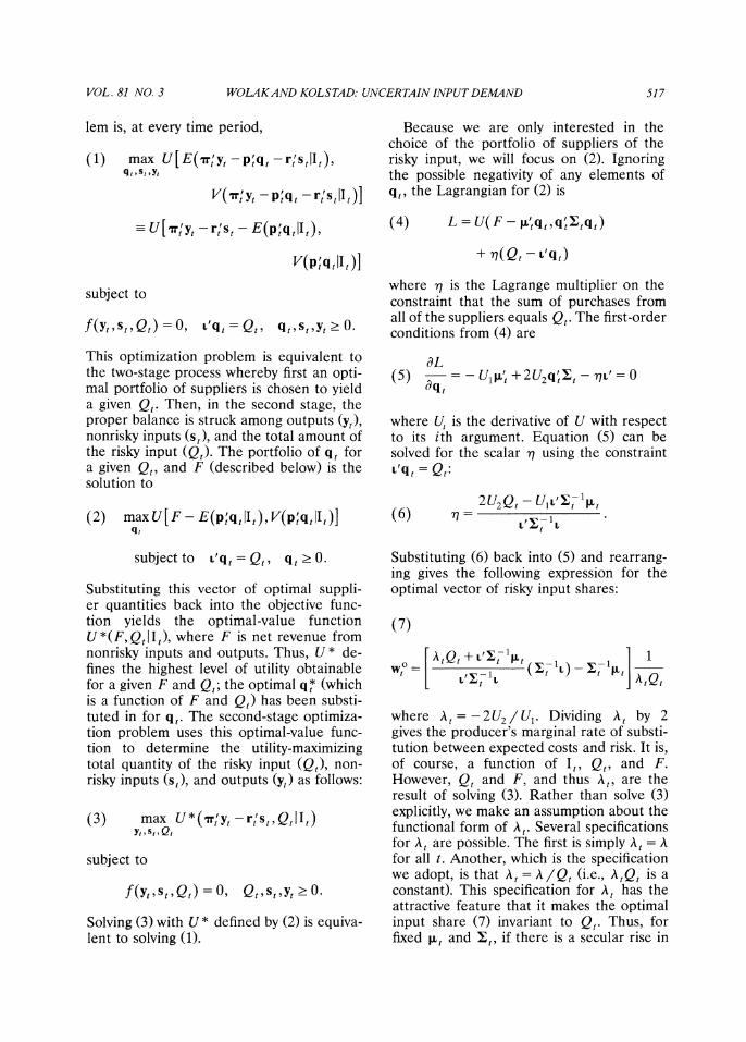
FIGURE 2. ACTUAL AND FITTED IMPORT PRICES IN THOUSANDS OF YEN PER METRIC TON OF STEAM COAL FOR THE UNITED STATES FROM ML MODEL

ESTIMATION

these figures is that fitted prices follow actual prices much more closely than fitted shares follow actual shares. Nevertheless, the model fits well enough not to predict negative shares for any observations in our sample, despite the fact that the actual shares, especially those for the Soviet Union, are extremely close to zero. In order to give some idea of the explanatory power of our model we computed an "R2" for each of the price functions and share equations estimated. Analogous to the way that it is defined for the linear-regression model, we define R2 1- (RSS/TSS), for

T

RSS= E( y) - 2) t = I

and

T

TSS= E (Y) t==1

where yt is the dependent variable of the

TABLE 6- R2 FOR PRICE AND SHARE EQUATIONS

R 2

Country Price Share

China 0.9527 0.3765 Soviet Union 0.8352 0.3501 United States 0.9339 0.3550 South Africa 0.9562 0.3632 Australia 0.9720 0.3642

equation, yt is the fitted value of yt, and -y is the sample mean of yt. In Table 6 we present these magnitudes for each price and share equation. Table 6 confirms the superior fit of the price equations. For the remainder of this section, we attempt to examine the validity of less restrictive models that include additional parameters or variables. We are unable to find substantial evidence against our structural model. Con- sequently, based on the specification tests discussed below, we conclude that this rather large unexplained variability in the


import shares is due either to factors that we have been unable to measure (which therefore cannot be incorporated into our model) or simply to nonsystematic deviations from optimizing behavior. We have modeled both of these phenomena by Et in (11).

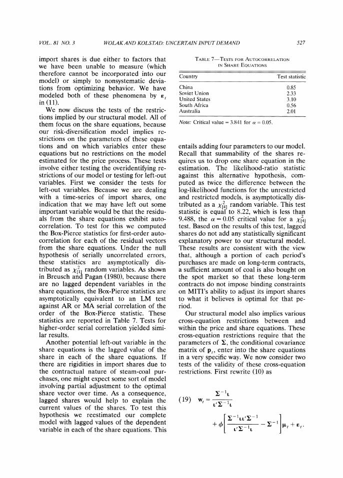
We now discuss the tests of the restrictions implied by our structural model. All of them focus on the share equations, because our risk-diversification model implies restrictions on the parameters of these equations and on which variables enter these equations but no restrictions on the model estimated for the price process. These tests involve either testing the overidentifying restrictions of our model or testing for left-out variables. First we consider the tests for left-out variables. Because we are dealing with a time-series of import shares, one indication that we may have left out some important variable would be that the residuals from the share equations exhibit autocorrelation. To test for this we computed the Box-Pierce statistics for first-order autocorrelation for each of the residual vectors from the share equations. Under the null hypothesis of serially uncorrelated errors, these statistics are asymptotically distributed as X' random variables. As shown in Breusch and Pagan (1980), because there are no lagged dependent variables in the share equations, the Box-Pierce statistics are asymptotically equivalent to an LM test against AR or MA serial correlation of the order of the Box-Pierce statistic. These statistics are reported in Table 7. Tests for higher-order serial correlation yielded similar results.

Another potential left-out variable in the share equations is the lagged value of the share in each of the share equations. If there are rigidities in import shares due to the contractual nature of steam-coal purchases, one might expect some sort of model involving partial adjustment to the optimal share vector over time. As a consequence, lagged shares would help to explain the current values of the shares. To test this hypothesis we reestimated our complete model with lagged values of the dependent variable in each of the share equations. This

TABLE 7-TESTS FOR AUTOCORRELATION IN SHARE EQUATIONS

Country Test statistic

China 0.85 Soviet Union 2.33 United States 3.10 South Africa 0.56 Australia 2.01

Note: Critical value = 3.841 for a = 0.05.

entails adding four parameters to our model. Recall that summability of the shares requires us to drop one share equation in the estimation. The likelihood-ratio statistic against this alternative hypothesis, computed as twice the difference between the log-likelihood functions for the unrestricted and restricted models, is asymptotically distributed as a XE41 random variable. This test statistic is equal to 8.22, which is less than

2 9.488, the a = 0.05 critical value for a X[4] test. Based on the results of this test, lagged shares do not add any statistically significant explanatory power to our structural model. These results are consistent with the view that, although a portion of each period's purchases are made on long-term contracts, a sufficient amount of coal is also bought on the spot market so that these long-term contracts do not impose binding constraints on MITI's ability to adjust its import shares to what it believes is optimal for that period.

Our structural model also implies various cross-equation restrictions between and within the price and share equations. These cross-equation restrictions require that the parameters of 1, the conditional covariance matrix of pt, enter into the share equations in a very specific way. We now consider two tests of the validity of these cross-equation restrictions. First rewrite (10) as

(19) wt =

+ 4 <t , 1 I t+


The unrestricted form of this set of equations is

(20) wt=A + B,t + Et

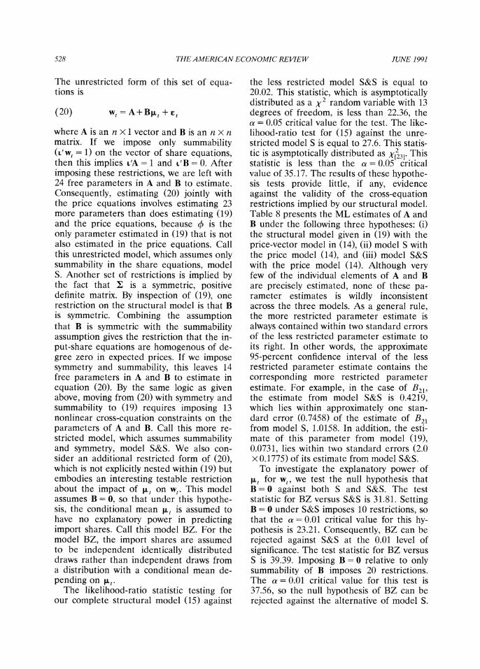
where A is an n x 1 vector and B is an n X n matrix. If we impose only summability ('Wt= 1) on the vector of share equations, then this implies L'A = 1 and L'B = 0. After imposing these restrictions, we are left with 24 free parameters in A and B to estimate. Consequently, estimating (20) jointly with the price equations involves estimating 23 more parameters than does estimating (19) and the price equations, because 4 is the only parameter estimated in (19) that is not also estimated in the price equations. Call this unrestricted model, which assumes only summability in the share equations, model S. Another set of restrictions is implied by the fact that I is a symmetric, positive definite matrix. By inspection of (19), one restriction on the structural model is that B is symmetric. Combining the assumption that B is symmetric with the summability assumption gives the restriction that the input-share equations are homogenous of de- gree zero in expected prices. If we impose symmetry and summability, this leaves 14 free parameters in A and B to estimate in equation (20). By the same logic as given above, moving from (20) with symmetry and summability to (19) requires imposing 13 nonlinear cross-equation constraints on the parameters of A and B. Call this more restricted model, which assumes summability and symmetry, model S&S. We also consider an additional restricted form of (20), which is not explicitly nested within (19) but embodies an interesting testable restriction about the impact of wt on wt. This model assumes B = 0, so that under this hypothesis, the conditional mean t,t is assumed to have no explanatory power in predicting import shares. Call this model BZ. For the model BZ, the import shares are assumed to be independent identically distributed draws rather than independent draws from a distribution with a conditional mean depending on Rt.

The likelihood-ratio statistic testing for our complete structural model (15) against

the less restricted model S&S is equal to 20.02. This statistic, which is asymptotically distributed as a X2 random variable with 13 degrees of freedom, is less than 22.36, the a = 0.05 critical value for the test. The likelihood-ratio test for (15) against the unrestricted model S is equal to 27.6. This statistic is asymptotically distributed as X 23]. This statistic is less than the a= 0.05 critical value of 35.17. The results of these hypothesis tests provide little, if any, evidence against the validity of the cross-equation restrictions implied by our structural model. Table 8 presents the ML estimates of A and B under the following three hypotheses: (i) the structural model given in (19) with the price-vector model in (14), (ii) model S with the price model (14), and (iii) model S&S with the price model (14). Although very few of the individual elements of A and B are precisely estimated, none of these parameter estimates is wildly inconsistent across the three models. As a general rule, the more restricted parameter estimate is always contained within two standard errors of the less restricted parameter estimate to its right. In other words, the approximate 95-percent confidence interval of the less restricted parameter estimate contains the corresponding more restricted parameter estimate. For example, in the case of B21, the estimate from model S&S is 0.4219, which lies within approximately one standard error (0.7458) of the estimate of B21 from model S, 1.0158. In addition, the estimate of this parameter from model (19), 0.0731, lies within two standard errors (2.0 x 0.1775) of its estimate from model S&S.

To investigate the explanatory power of Ft for wt, we test the null hypothesis that B = 0 against both S and S&S. The test statistic for BZ versus S&S is 31.81. Setting B = 0 under S&S imposes 10 restrictions, so that the a = 0.01 critical value for this hypothesis is 23.21. Consequently, BZ can be rejected against S&S at the 0.01 level of significance. The test statistic for BZ versus S is 39.39. Imposing B = 0 relative to only summability of B imposes 20 restrictions. The a = 0.01 critical value for this test is 37.56, so the null hypothesis of BZ can be rejected against the alternative of model S.


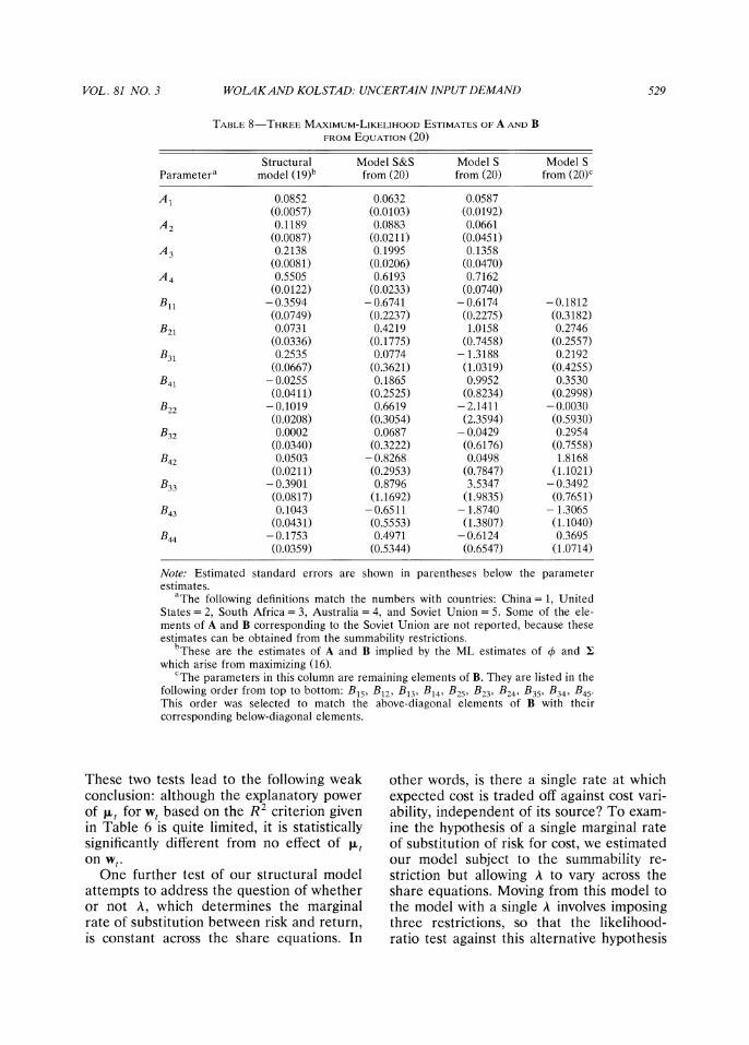
TABLE 8-THREE MAxIMuM-LIKELIHooD ESTIMATES OF A AND B FROM EQUATION (20)

Structural Model S&S Model S Model S Parametera model (19)b from (20) from (20) from (20)C

A1 0.0852 0.0632 0.0587 (0.0057) (0.0103) (0.0192)

A2 0.1189 0.0883 0.0661 (0.0087) (0.0211) (0.0451)

A3 0.2138 0.1995 0.1358 (0.0081) (0.0206) (0.0470)

A4 0.5505 0.6193 0.7162 (0.0122) (0.0233) (0.0740)

Bll -0.3594 -0.6741 -0.6174 -0.1812 (0.0749) (0.2237) (0.2275) (0.3182)

B21 0.0731 0.4219 1.0158 0.2746 (0.0336) (0.1775) (0.7458) (0.2557)

B31 0.2535 0.0774 -1.3188 0.2192 (0.0667) (0.3621) (1.0319) (0.4255)

B41 -0.0255 0.1865 0.9952 0.3530 (0.0411) (0.2525) (0.8234) (0.2998)

B22 -0.1019 0.6619 -2.1411 -0.0030 (0.0208) (0.3054) (2.3594) (0.5930)

B32 0.0002 0.0687 - 0.0429 0.2954 (0.0340) (0.3222) (0.6176) (0.7558)

B42 0.0503 -0.8268 0.0498 1.8168 (0.0211) (0.2953) (0.7847) (1.1021)

B33 -0.3901 0.8796 3.5347 -0.3492 (0.0817) (1.1692) (1.9835) (0.7651)

B43 0.1043 -0.6511 -1.8740 -1.3065 (0.0431) (0.5553) (1.3807) (1.1040)

B44 -0.1753 0.4971 -0.6124 0.3695 (0.0359) (0.5344) (0.6547) (1.0714)

Note: Estimated standard errors are shown in parentheses below the parameter estimates.

aThe following definitions match the numbers with countries: China= 1, United States = 2, South Africa = 3, Australia = 4, and Soviet Union = 5. Some of the elements of A and B corresponding to the Soviet Union are not reported, because these estimates can be obtained from the summability restrictions.

bThese are the estimates of A and B implied by the ML estimates of 0 and I which arise from maximizing (16).

cThe parameters in this column are remaining elements of B. They are listed in the following order from top to bottom: B15, B12, B13, B14, B25, B23, B24, B35, B34, B45- This order was selected to match the above-diagonal elements of B with their corresponding below-diagonal elements.

These two tests lead to the following weak conclusion: although the explanatory power of w, for w, based on the R2 criterion given in Table 6 is quite limited, it is statistically significantly different from no effect of wt on wt.

One further test of our structural model attempts to address the question of whether or not A, which determines the marginal rate of substitution between risk and return, is constant across the share equations. In

other words, is there a single rate at which expected cost is traded off against cost variability, independent of its source? To examine the hypothesis of a single marginal rate of substitution of risk for cost, we estimated our model subject to the summability restriction but allowing A to vary across the share equations. Moving from this model to the model with a single A involves imposing three restrictions, so that the likelihood- ratio test against this alternative hypothesis


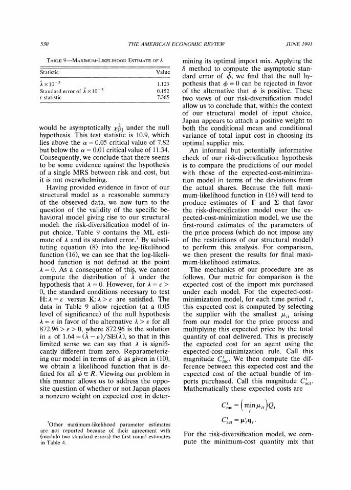
TABLE 9-MAXIMUM-LIKELIHOOD ESTIMATE OF A

Statistic Value

A Xi10-3 1.123 Standard error of A X 10- 0.152 t statistic 7.365

would be asymptotically X[3] under the null hypothesis. This test statistic is 10.9, which lies above the a = 0.05 critical value of 7.82 but below the a = 0.01 critical value of 11.34. Consequently, we conclude that there seems to be some evidence against the hypothesis of a single MRS between risk and cost, but it is not overwhelming.

Having provided evidence in favor of our structural model as a reasonable summary of the observed data, we now turn to the question of the validity of the specific be- havioral model giving rise to our structural model: the risk-diversification model of input choice. Table 9 contains the ML estimate of A and its standard error.7 By substituting equation (8) into the log-likelihood function (16), we can see that the log-likelihood function is not defined at the point A = 0. As a consequence of this, we cannot compute the distribution of A under the hypothesis that A = 0. However, for A = E > 0, the standard conditions necessary to test H: A = E versus K: A > e are satisfied. The data in Table 9 allow rejection (at a 0.05 level of significance) of the null hypothesis A = E in favor of the alternative A > E for all 872.96 > e > 0, where 872.96 is the solution in E of 1.64 = (A - E)/SE(A), so that in this limited sense we can say that A is significantly different from zero. Reparameteriz- ing our model in terms of 0 as given in (10), we obtain a likelihood function that is defined for all 0 E R. Viewing our problem in this manner allows us to address the oppo- site question of whether or not Japan places a nonzero weight on expected cost in deter-

mining its optimal import mix. Applying the 8 method to compute the asymptotic standard error of b, we find that the null hypothesis that + = 0 can be rejected in favor of the alternative that 4 is positive. These two views of our risk-diversification model allow us to conclude that, within the context of our structural model of input choice, Japan appears to attach a positive weight to both the conditional mean and conditional variance of total input cost in choosing its optimal supplier mix.

An informal but potentially informative check of our risk-diversification hypothesis is to compare the predictions of our model with those of the expected-cost-minimization model in terms of the deviations from the actual shares. Because the full maximum-likelihood function in (16) will tend to produce estimates of r and I that favor the risk-diversification model over the expected-cost-minimization model, we use the first-round estimates of the parameters of the price process (which do not impose any of the restrictions of our structural model) to perform this analysis. For comparison, we then present the results for final maximum-likelihood estimates.

The mechanics of our procedure are as follows. Our metric for comparison is the expected cost of the import mix purchased under each model. For the expected-cost- minimization model, for each time period t, this expected cost is computed by selecting the supplier with the smallest Ait arising from our model for the price process and multiplying this expected price by the total quantity of coal delivered. This is precisely the expected cost for an agent using the expected-cost-minimization rule. Call this magnitude ct c We then compute the difference between this expected cost and the expected cost of the actual bundle of imports purchased. Call this magnitude Ctct. Mathematically these expected costs are

=c (Ci ninit )Qt

ct = Ut qt act

For the risk-diversification model, we compute the minimum-cost quantity mix that

7Other maximum-likelihood parameter estimates are not reported because of their agreement with (modulo two standard errors) the first-round estimates in Table 4.


yields the same conditional variance of cost as the actual quantities purchased. Define V, = qt q, as the conditional variance of the actual quantity vector qt. For each time period t, this minimum-conditional-cost quantity mix is the solution to

(21) min q'tt q

subject to Vt = q'lq and Qt = q'L.

If q' is the solution to (21), then Ct the is rd'

minimum cost of a quantity mix with variance Vt, is equal to q'tLt. We compute ct - Ct and Ct - C'd for all observa-

tions. Because the absolute magnitudes of these differences in costs provide little intuition, we instead focus on the ratio of these differences to the actual expected cost. The sample average of (Ct - Ct c)/ Cct, is approximately 0.169. This means that, averaging over our sample, the expected total import cost associated with the minimum- expected-cost criterion is 16.9 percent below actual expected import costs. The sample average of (Ct - Ctd)/Ct is 0.035, so that, averaging over our sample, the minimum-cost import bundle having the same variance as the actual bundle imported, has an expected cost that is 3.5 percent below actual import costs. If we compute these two magnitudes using the final (as opposed to first-round) estimates of r and 1, then the two numbers become 16.7 percent and 1.0 percent, respectively. Although there is an improvement in the conformity of the data to the risk-diversification model as a result of imposing the cross-equation restrictions between the share and price equations in the full maximum-likelihood procedure, the divergence of actual expected costs from those predicted by the risk-diversification hypothesis are minor when compared to the divergence of actual expected costs from those predicted by the expected-cost- minimization hypothesis. Although, as discussed above, the risk-diversification hypothesis cannot be explicitly tested due to the fact that the likelihood function is not well-defined at the point A = 0, the evidence presented here suggests that it is a

superior model to the expected-cost-minimization model for describing the Japanese steam-coal import market.

V. Implications of the Risk-Diversification Model of Input Demand

We now examine the empirical implications of this estimated model of short-run input demand under price uncertainty. We are concerned with three general questions. What is the size of the risk premium associated with steam coal imported to Japan? What relationships between the observed prices and shares does the risk-diversification model imply, and are these relationships consistent with the observed data? How well does this model of input choice explain the three time-series properties of supplier prices and shares of steam coal imported to Japan discussed in the Intro- duction?

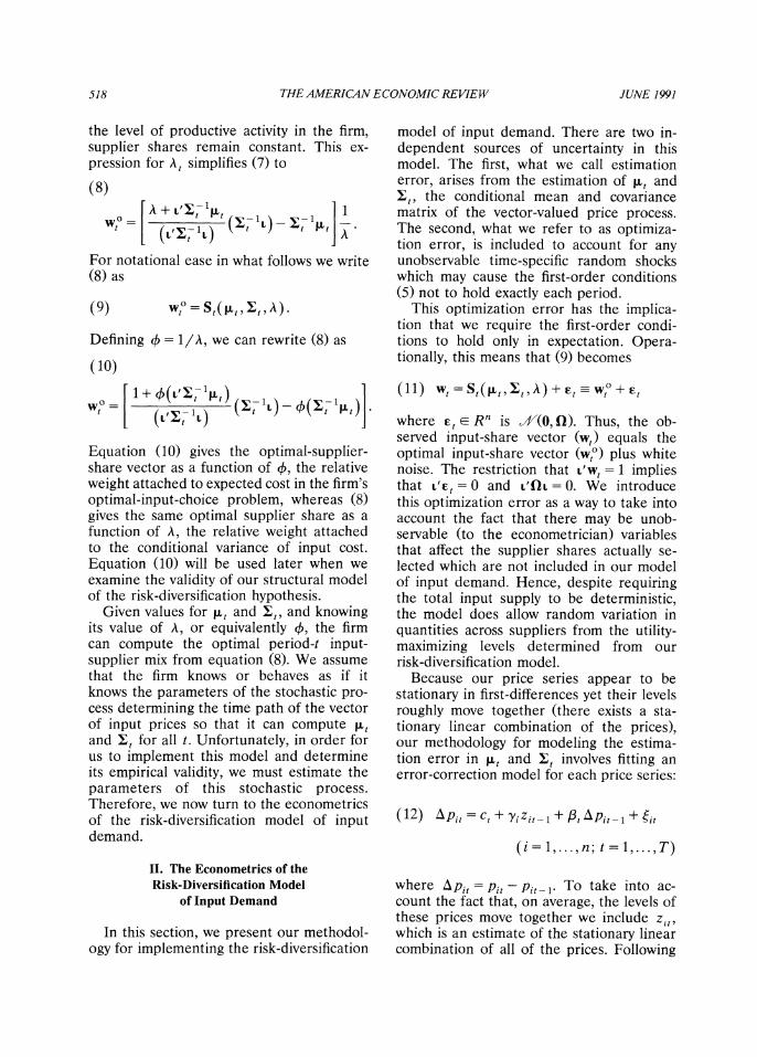
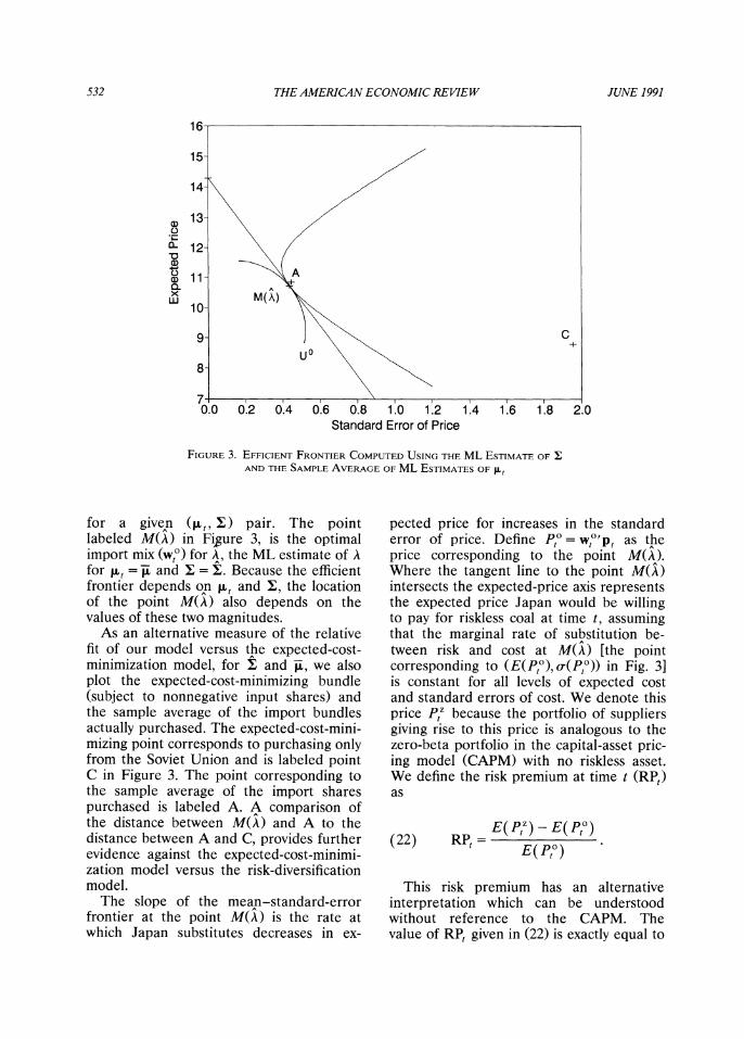
We first consider the question of the size of the risk premium on imported coal. To derive this magnitude, consider the mean- price versus standard-error-of-price frontier, plotted in Figure 3. Such frontiers can be plotted for each (t, 1) pair in our sample. Figure 3 is constructed using I, the maximum-likelihood estimate of I and ,u, the sample mean of t,u(r, It), as a representative value of Lt, where r is the ML estimate of r. Define Pp(w) = w'pt = w5= WiPit as the actual weighted average

price of steam-coal imports at time t, where 5= lw 1. Let E(Pp (W))-Wt tt equal the

expectation condition'al on It of Pp(w) and cr(PP(w)) -w' wt equal its variance conditional on It" The mean-standard-error frontier given in Figure 3 comprises the set of (E(Pp), o-(PP,)) pairs such that o-(Pp(w)) is minimized over w subject to the constraints L'W = 1 and E(Pp (w)) = K, where K is some positive constant. Once a value of A is specified, the solution of (2) implies a point on the mean-standard-error frontier corresponding to the optimal input mix

8For the remainder of this section, all expectations and variances are conditional on It, the firm's information set at time t.


16-

15-

14-

- 12 l

AND THA

9- 10~~~~~~~

8-

7- 0.0 0.2 0.4 0.6 0.8 1.0 1.2 1.4 1.6 1.8 2.0

Standard Error of Price

FIGURE 3. EFFICIENT FRONTIER COMPUTED USING THE ML ESTIMATE OFI AND THE SAMPLE AVERAGE OF ML ESTIMATES OF ILt

for a given (,'t, :) pair. The point labeled M(A) in Fi,gure 3, is the optimal import mix (wa) for A, the ML estimate of A for , = ,u and I = :. Because the efficient frontier depends on 1,u and :, the location of the point M(A) also depends on the values of these two magnitudes.

As an alternative measure of the relative fit of our model versus the expected-cost- minimization model, for I and ,u, we also plot the expected-cost-minimizing bundle (subject to nonnegative input shares) and the sample average of the import bundles actually purchased. The expected-cost-minimizing point corresponds to purchasing only from the Soviet Union and is labeled point C in Figure 3. The point corresponding to the sample average of the import shares purchased is labeled A. A comparison of the distance between M(A) and A to the distance between A and C, provides further evidence against the expected-cost-minimization model versus the risk-diversification model.

The slope of the mean-standard-error frontier at the point M(A) is the rate at which Japan substitutes decreases in ex-

pected price for increases in the standard error of price. Define P/? = w/I'p, as the price corresponding to the point M(A). Where the tangent line to the point M(A intersects the expected-price axis represents the expected price Japan would be willing to pay for riskless coal at time t, assuming that the marginal rate of substitution between risk and cost at M(A) [the point corresponding to (E(Pto),a(Pto)) in Fig. 3] is constant for all levels of expected cost and standard errors of cost. We denote this price Pt' because the portfolio of suppliers giving rise to this price is analogous to the zero-beta portfolio in the capital-asset pricing model (CAPM) with no riskless asset. We define the risk premium at time t (RP,) as

(22) P~ =E(Ptz) - E(Pto) ( 22) RPt- E(Pto)

This risk premium has an alternative interpretation which can be understood without reference to the CAPM. The value of RPt given in (22) is exactly equal to


0.55-

0.5

c o 0451

Ei 0.4- E a)

, 0.35-

0.3-

0.25 II4 1 5 10 15 '206 25' 30 3 40 4 49

Time In Months (First Period=May 1983)

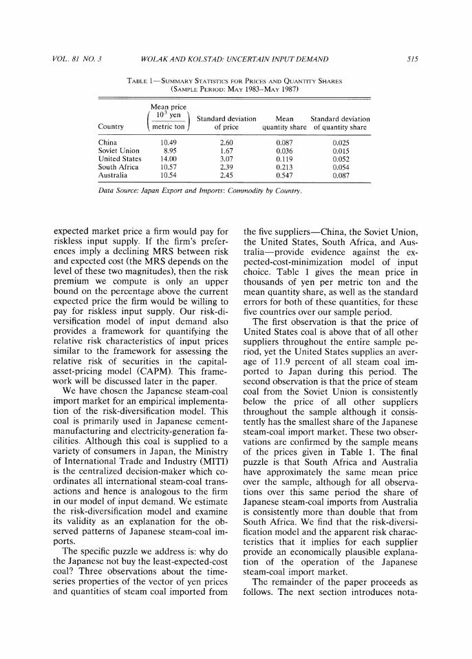
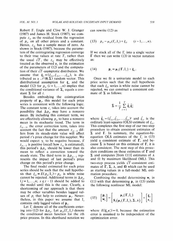
FIGURE 4. RISK PREMIUM (RP,) FOR SAMPLE PERIOD

- El,O(p,O), the negative of Japan's elasticity of import price risk with respect to expected import price. This elasticity is defined as

d log( P,?)

where

t = wt/F't and o(Pt ) =(wt 'wt )

and where wto is defined in (7). In terms of the parameters of our structural model,

cr ( Pto) A

p0A,oa(pt) ot

Although EA 0, (po) = - RPt, we still need to compute E(Ptz) in order to present other extensions of the analogy between the risk- diversification model and the CAPM.

An alternative methodology for computing Ptz uses the intuition of the zero-beta CAPM. The price Ptz arises from the portfolio of suppliers (weighted average price),

which has no market risk (market risk is defined as covariance with P/- w?'p,). To compute this portfolio, we solve for the minimum-variance weighted-average price subject to the constraint that its covariance with P/? is zero. The Lagrangian for this optimization problem takes the form

(24) L = lwtzwwz + ( 2wtzwto)

+ v( L'Wtz)

where wtz is the independent variable and 'q and v are Lagrange multipliers associated with the constraints that the covariance of Ptz with Pto is zero and that L'Wtz is equal to 1. The solution to (24) is

(25) wtz= 1 - (WO'IWto) ('I- 1)L

Using (25) and our ML parameter estimates, we can compute E(Pto)= =?t and E(PtZ) for all of our observations.

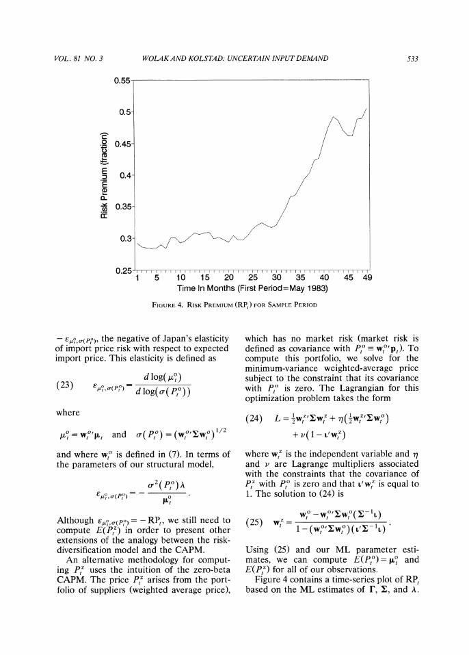
Figure 4 contains a time-series plot of RPt based on the ML estimates of r, 1, and A.


This risk premium ranges from 29 percent to 50 percent over the sample period, imply- ing that Japan seems willing to pay 29-50 percent above the current market price for a supply of coal having no price risk. Recall that this calculation assumes that the marginal rate of substitution between risk and cost is constant over all risks and costs. If Japan's preferences for risk entail a declining marginal rate of substitution of risk for cost, then these numbers only represent an upper bound on the risk premium at time t. For some utility functions, they could be extremely conservative bounds on the risk premium. To illustrate this point, Fig- ure 3 contains an indifference curve tangent to M(A) which exhibits a declining MRS.

By inspection of Figure 4, this risk premium exhibits an increasing time trend. A risk premium that increases with time is consistent with the view that, as Japan becomes more and more dependent on foreign sources of steam coal, as has been the case in recent years, the amount above the current weighted average market price Japan is willing to pay for coal with no price risk should increase. The interpretation of our results that is based on the elasticity of substitution between risk and cost [equation (23)] allows the following statement: at the point M(A), the loss in utility to Japan from a 1-percent increase in o-(Pj0) can be exactly offset by a 0.29-0.50-percent decrease in At, depending on the time period in the sample.

We now turn to the issue of how well our risk-diversification model of input demand explains the time path of Japan's steam-coal import shares. To treat this issue, we first present one further implication of our model of input choice and discuss the applicability of this implication to our data. From equation (11), we know that the expected value of the observed vector of quantity shares is equal to the optimal vector of quantity shares based on txt, 1, and A. More precisely, the expectation of wt is the vector of optimal import shares for Lt, , and A, so that

E(wti) = S(tat, s hAt) = wta.

This condition states that the expectation

of the actual import share Japan chooses is a point on the efficient [E(Pp),o-(Pp)] frontier. Using w', the optimal import-share vector for period t, we can construct a measure of risk for each supplier's price relative to P,0 = wt,'pt analogous to the market- specific measure of risk for each security in the CAPM. For this reason, we denote the market-specific measure of risk for supplier i in period t by P,t and define it as

Cov( P0, Pl) Var( Pt7)

where plt is supplier i's price. The covariance and variance in the expression for pit

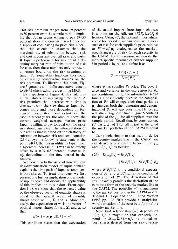
are conditional on It, the information set at time t. Consequently, because the composi- tion of Pt' will change each time period as wt changes, both the numerator and denom- inator of 83t will vary over time. Hence, 3t will also change over time. Figure 5 contains the plot of the f13t for all suppliers over the sample period. Recall that, by construction, Pto has a 8t of 1 for all t, just as the : of the market portfolio in the CAPM is equal to 1.

Using logic similar to that used to derive the security market line in the CAPM, we can derive a relationship between the 8it and E(plt II) as follows:

(26) E(pt IIt) = E(PtzlIt)

+ [E(PtoIt)- E(PzIIt)II8it

where E(Pto I It) is the conditional expectation of Pto and E(PtzI It) is the conditional expectation of Pt. The derivation of this result exactly parallels the derivation of the zero-beta form of the security market line in the CAPM. The portfolio wt? is analogous to the market portfolio in the CAPM model. Thomas E. Copeland and J. Fred Weston (1983 pp. 198-200) provide a straightfor- ward derivation of the zero-beta form of the security market line.

Note that relationship (26) depends on E(Pt?llt), a magnitude that explicitly depends on S(Qit, X, A) = wto, the optimal import shares derived from our risk-diversifi-


2-

1 .5- co

~~~~0 ~ 0

co 4- I a)

-0.5 I 1 r 1 5 10 15 20 25 30 35 40 45 49

Time In Months (First Period=May 1983) China - USSR o U.S.

South Africa Australia

FIGURE 5. ,B'S OVER SAMPLE PERIOD, COMPUTED FROM EFFICIENT SHARES (Pa)

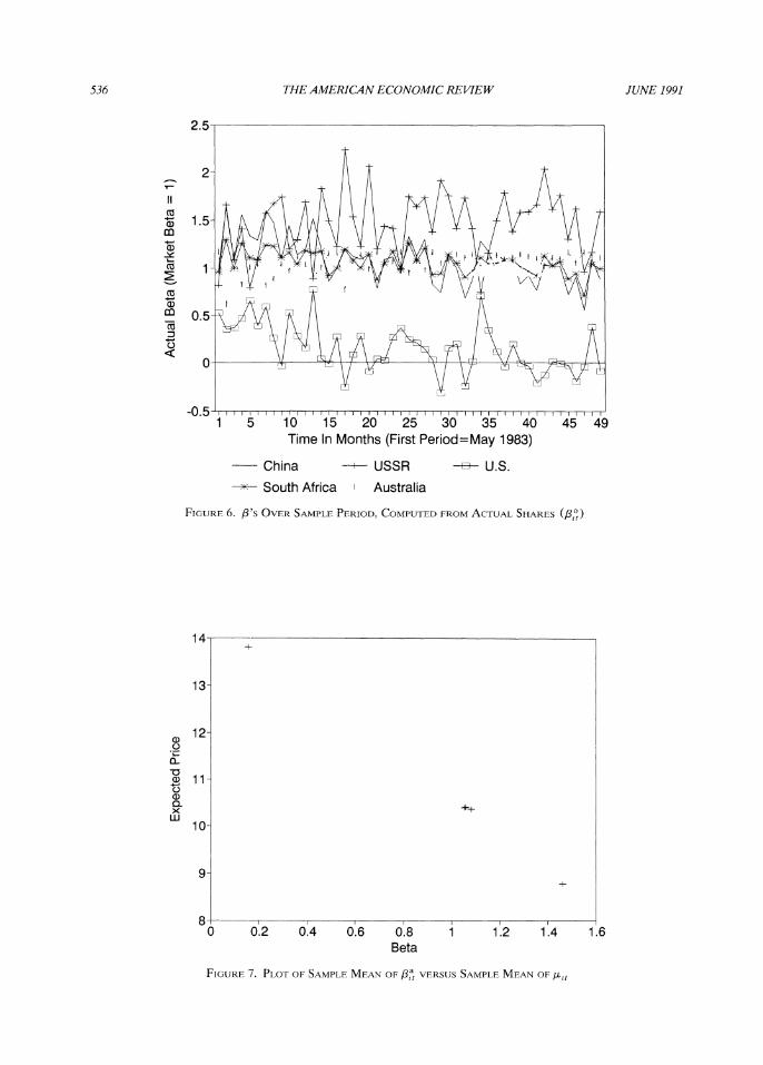
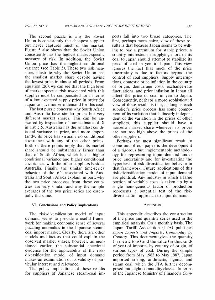
cation model.9 Hence, another check of the reasonableness of our structural model is to recompute the /it using w, instead of w,? to see whether or not there is a linear relationship between these 8,, (call them ,3t) and E(pitlIt), as suggested by equation (26). Figure 6 contains a plot of the pa. The levels and pattern of the 3ia over time are quite similar to those followed by the fit based on w'0, but the time series of I3' is clearly more volatile than that of fit. In Figure 7, we plot the sample average of the /8a against the sample mean of the ,it. Although there are only five points on the plot, the relationship between the sample means of the yit and 8a is very well ap- proximated by a straight line. Consequently, using the observed share data to construct the risk measures, a linear relation similar

to that in (26) seems to hold with E(PO0 II) replaced by E(Pj II), where P, = wl'p,.

We are now in a position to address the three puzzles presented in the Introduction. The first puzzle is why the United States remains in the market despite its consistently high price. Figure 5 shows that the United States consistently has the lowest market-specific measure of risk associated with it. In fact, :3 for the United States is negative in some periods, and for the most part it hovers around zero, indicating that United States coal is a good hedge against variations in the market price of coal. The very low market-specific risk associated with the price of U.S. coal explains why the United States services a sizeable share of the market even though its price path lies above those of the other four countries and has the second-largest conditional variance (see Table 5). Furthermore, the negative elements in the United States' row and column in I explains how this ,B close to zero comes about.

9We are grateful to a referee for suggesting the following procedure to examine validity of equation (26).


2.5

CIO

co)

1 5 10 15 201 25 30 35 40 45 49 Time In Months (First Period=May 1983)

China ---USSR -n- U.S. ->-- South Africa Australia

FIGURE 6.: 'S OVER SAMPLE PERIOD, COMPUTED PROM ACTUAL SHARES (/38',)

14 +

13-

a,12-

Ci) a ~~~~~~~~~++

8 I

10- LI-

0 0.2 0.4 0.6 0.8 1 1.2 1.4 1.6 Beta

FIGURE 7. PLOT OP SAMPLE MEAN OP CMU VERSUmS SAMPLE MEAN OP8't


The second puzzle is why the Soviet Union is consistently the cheapest supplier but never captures much of the market. Figure 5 also shows that the Soviet Union consistently has the highest market-specific measure of risk. In addition, the Soviet Union price has the highest conditional variance (see Table 5). These two risk measures illustrate why the Soviet Union has the smallest market share despite having the lowest price in almost all periods. From equation (26), we can see that the high level of market-specific risk associated with this supplier must be compensated for in terms of a low expected supply price in order for Japan to have nonzero demand for this coal.

The last puzzle concerns why South Africa and Australia have similar prices but very different market shares. This can be an- swered by inspection of our estimate of I in Table 5. Australia has the smallest conditional variance in price, and more impor- tantly, its price has virtually no conditional covariance with any of the other prices. Both of these points imply that its market share should be substantially larger than that of South Africa, which has a higher conditional variance and higher conditional covariances with the other suppliers besides Australia. Finally, the similar time-series behavior of the ,3's associated with Aus- tralia and South Africa explain, in part, why the two price processes from these countries are very similar and why the sample averages of the two price series are essen- tially the same.

VI. Conclusions and Policy Implications

The risk-diversification model of input demand seems to provide a useful framework for making economic sense of several puzzling anomalies in the Japanese steam- coal import market. Clearly, there are other models and factors that could explain the observed market shares; however, as mentioned earlier, the substantial anecdotal evidence for the applicability of the risk- diversification model of input demand makes an examination of its validity of par- ticular interest and relevance.

The policy implications of these results for suppliers of Japanese steam-coal im-

ports fall into two broad categories. The first, perhaps more naive, view of these results is that because Japan seems to be willing to pay a premium for stable prices, a country interested in supplying more of its coal to Japan should attempt to stabilize its price of coal in yen to Japan. This view ignores the fact that much of the price uncertainty is due to factors beyond the control of coal suppliers. Supply interrup- tions, domestic price inflation in the country of origin, demurrage costs, exchange-rate fluctuations, and price inflation in Japan all affect the price of coal in yen to Japan. Consequently, perhaps a more sophisticated view of these results is that, as long as each supplier's price process has some compo- nent of its variation that is linearly independent of the variation in the prices of other suppliers, this supplier should have a nonzero market share whenever its prices are not too high above the prices of the other suppliers.

Perhaps the most significant result to come out of our paper is the development of a rigorous but implementable methodology for representing input demand under price uncertainty and for investigating the hypothesis of risk-diversification behavior in that framework. Future applications of this risk-diversification model of input demand are plentiful. Any industry in which a large portion of variable costs is taken up by a single homogeneous factor of production represents a potential test of the risk- diversification approach to input demand.

APPENDIX

This appendix describes the construction of the price and quantity series used in the empirical analysis. On a monthly basis, The Japan Tariff Association (JTA) publishes Japan Exports and Imports, Commodity by Country. This document gives the quantity (in metric tons) and the value (in thousands of yen) of imports, by country of origin, of various types of coal. During the sample period from May 1983 to May 1987, Japan imported coking, anthracite, lignite, and steam coal, which the JTA further decom- posed into eight commodity classes. In terms of the Japanese Ministry of Finance's Com-


modity Classification for Foreign Trade Statistics classification system, steam coal is defined as commodity numbers 27.01-129 and 27.01-199. Consequently, to construct the total quantity and value of steam-coal imports from each country for each month, we computed the quantity and value totals for each country over these two commodity numbers. The price in thousands of yen per metric ton for a given country is obtained by dividing total value of shipments in the month by the total quantity of shipments in that month. If contacted at the address given in the initial footnote, the first author is willing to provide a machine-readable file containing these price and quantity data on a floppy diskette in DOS format.

REFERENCES

Batra, Raveendra N. and Ullah, Aman, "Com- petitive Firm and the Theory of Input Demand under Price Uncertainty," Jour- nal of Political Economy, June 1974, 82, 537-48.

Berndt, Ernst K., Hall, Bronwyn H., Hall, Robert E. and Hausman, Jerry A., "Estimation and Inference in Nonlinear Structural Mod- els," Annals of Economic and Social Mea- surement, October 1974, 3, 653-65.

Blair, Roger D., "Random Input Prices and the Theory of the Firm," Economic In- quiry, June 1974, 12, 214-26.

Breusch, Trevor S. and Pagan, Adrian R., "The Lagrange Multiplier Test and its Applica- tion to Model Specification in Economet- rics," Review of Economics Studies Jan- uary 1980 (Econometrics Issue), 47, 239-53.

Copeland, Thomas E. and Weston, J. Fred, Fi- nancial Theory and Corporate Policy, Reading, MA: Addison-Wesley, 1983.

Dickey, David A. and Fuller, Wayne A., "Distri- bution of the Estimators for Autoregres- sive Time Series with a Unit Root," Jour- nal of the American Statistical Association, June 1979, 74, 427-31.

Durbin, James M., "Testing for Serial Corre- lation in Least Squares Regression When Some of the Regressors Are Lagged De- pendent Variables," Econometrica, May 1970, 38, 410-21.

Engle, Robert F., "Autoregressive Condi- tional Heteroscedasticity with Estimates of the Variance of United Kingdom In- flation," Econometrica, July 1982, 50, 987-1007.

and Granger, Clive W. J., "Co-integra- tion and Error Correction: Representa- tion, Estimation, and Testing," Econo- metrica, March 1987, 55, 251-76.

and Yoo, Byung S., "Forecasting and Testing in Co-integrated Systems," Jour- nal of Econometrics, May 1987, 35, 143-60.

Fuller, Wayne A., Introduction to Statistical Time Series, New York: Wiley, 1976.

Johansen, Soren, "Statistical Analysis of Cointegration Vectors," Journal of Eco- nomic Dynamics and Control, June/Sep- tember 1988, 12, 231-54.

Lehmann, Erich L., Theory of Point Estima- tion, New York: Wiley, 1983.

Sandmo, Agnar, "Competitive Firm under Price Uncertainty," American Economic Review, March 1971, 61, 65-73.

Stock, James H., "Asymptotic Properties of Least Squares Estimators of Cointegrat- ing Vectors," Econometrica, September 1987, 55, 1035-56.

Tukenmez, Ercan and Tuck, Nancy, "Coal- Exporting Countries: The Asian Market," U.S. Department of Energy Report DOE/ EIA-0462, Washington, DC: U.S. Gov- ernment Printing Office, 1984.

West, Kenneth D., "Asymptotic Normality, When Regressors Have a Unit Root," Econometrica, November 1988, 56, 1397- 1418.

Wu, Yuan-li, Japan's Search for Oil, Stan- ford, CA: Hoover Institution Press, 1977.

Japan Export and Imports: Commodity by Country, Tokyo: Japan Tariff Association, monthly, 1983-1987.

Ministry of International Trade and Industry, The MITI Handbook, Tokyo: Japan Trade and Industry Publicity, Inc., 1979/1980.

TEX Report, 1986 Coal Manual, Tokyo: TEX Report, Ltd., 1986.

United States Department of Energy, " Interim Report of the Interagency Coal Export Task Force," U.S. Department of Energy Report DOE/FE-0012, Washington, DC: U.S. Government Printing Office, 1981.

Documents

A Model of Homogeneous Input Demand Under Price Uncertaintyweb.stanford.edu/group/fwolak/cgi-bin/sites/default/files/files/... · A Model of Homogeneous Input Demand Under Price Uncertainty