Embed Size (px)
Citation preview
Multivariate Analysis of Regression Patterns
Timothy DelSole and Xiaosong Yang
George Mason University, Fairfax, Va andCenter for Ocean-Land-Atmosphere Studies, Calverton, MD
July 25, 2010
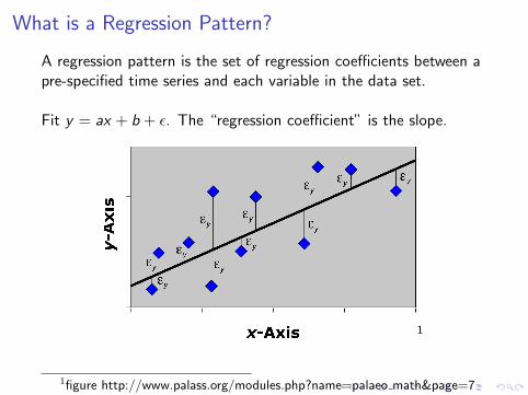
What is a Regression Pattern?
A regression pattern is the set of regression coefficients between apre-specified time series and each variable in the data set.
Fit y = ax + b + ε. The “regression coefficient” is the slope.
1
1figure http://www.palass.org/modules.php?name=palaeo math&page=7
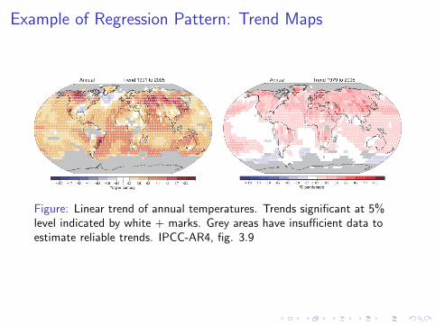
Example of Regression Pattern: Trend Maps
Figure: Linear trend of annual temperatures. Trends significant at 5%level indicated by white + marks. Grey areas have insufficient data toestimate reliable trends. IPCC-AR4, fig. 3.9
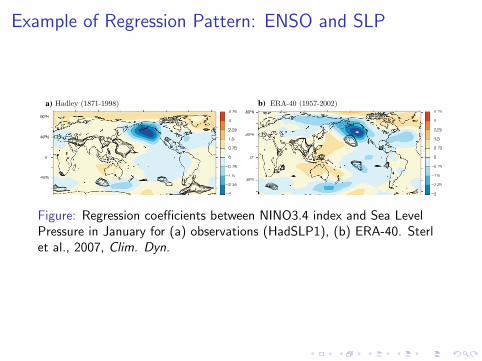
Example of Regression Pattern: ENSO and SLP
tween pressure p and N34, and rp is the observed standarddeviation of p. By construction g!t" # $p!t" % rN34!t"&=!rp!!!!!!!!!!!!!1% c2
p" is that part of p that is unrelated to ENSO, i.e.,
corr(N34, g) = 0. It has zero mean and unit standarddeviation.
We now consider sub-periods PW!t" # $t %W=2;t 'W=2& ( $0; T& of lengthW of the whole period of lengthT. Following Van Oldenborgh and Burgers (2005) we use a
length of W = 25 years throughout this paper. This is long
enough to resolve ENSO and short enough not to beinfluenced by low-frequency (decadal and longer) varia-
tions. For notational convenience we drop the subscript Win what follows. A tilde is used to denote time series re-stricted to a sub-period, e.g., ~pt0!t" # ~p!t" # p!tjt 2 P!t0"";where the subscript t¢ has been dropped for convenience.
Using (Eq. 6) the regression of ~p on ~N34 then reads
~r!t" # regr! ~N34; ~p" # r ' rp!!!!!!!!!!!!!1% c2
p~rg!t"; !2"
where ~rg!t" # regr!~N34; ~g": Apart from the factorrp
!!!!!!!!!!!!!1% c2
pthis quantity is the deviation of the regression
during P(t) from its long-term mean value r. Obviously,~rg!t" ! 0 in the limit W fi T, but ~rg!t" can be non-zeroif the sub-period is so short that it is not influenced by low-
frequency variations in the background state. If ~rg!t" is
distributed around zero the long-term mean regression r isa good approximation of ~rg!t" 8t:
The statement ‘‘the strength of the teleconnection does
not change significantly with time’’ means that the varia-
tions of ~r!t" are small in the sense that they are explainableby chance—~rg!t" will vary even for a purely stochastic g(t).To test this we use a Monte Carlo approach. We replace
g(t) in (Eq. 1) by a Gaussian process (random numbergenerator from Numerical Recipes; Press et al. 1992) withthe same statistical properties (zero mean, unit standard
deviation) and simulate the probability density function(PDF) of ~r!t" by using a large number (1,000, say) of
stochastic series of g. If the observed values of ~r!t" lie
within the PDF they are ‘‘small’’, and the strength of theteleconnections does not change. The time series ~r!t" is
stationary (more precisely: nonstationarity cannot be re-
jected) and observed variations in ~r!t" can be explained asthe result of a stochastic process brought about by the
combined action of all non-ENSO processes, represented
by g. Conversely, if the observed values of ~r!t" lie outsidethe PDF we can conclude that the teleconnections them-
selves have changed.
The actual test builds upon these general considerations,but differs in two points. First, we do not use regression but
correlation, transformed to Fisher’s z values: z # 12 log
!1' c"=!1% c": This quantity is unbounded, estimates aremore normally distributed around the true value, and
the variance is to a first approximation independent of
c. Second, instead of dealing directly with z we use
a) Hadley (1871-1998) b) ERA-40 (1957-2002)
c) Speedy (1881-2002) d) ECHAM5/MPI-OM (1860-2000)
Fig. 2 As Fig. 1, but regression instead of correlations. Units, hPa/K
472 A. Sterl et al.: On the robustness of ENSO teleconnections
123
Figure: Regression coefficients between NINO3.4 index and Sea LevelPressure in January for (a) observations (HadSLP1), (b) ERA-40. Sterlet al., 2007, Clim. Dyn.
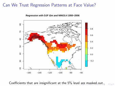
Can We Trust Regression Patterns at Face Value?
−160 −140 −120 −100 −80 −60
2030
4050
6070
80
lon
lat
−0.2
0.0
0.2
0.4
0.6
0.8
Regression with DJF t2m and NINO3.4 1950−2006
Coefficients that are insignificant at the 5% level are masked out.
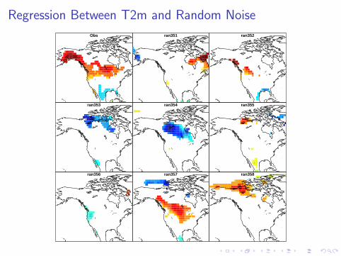
Regression Between T2m and Random Noise
Obs ran351 ran352
ran353 ran354 ran355
ran356 ran357 ran358
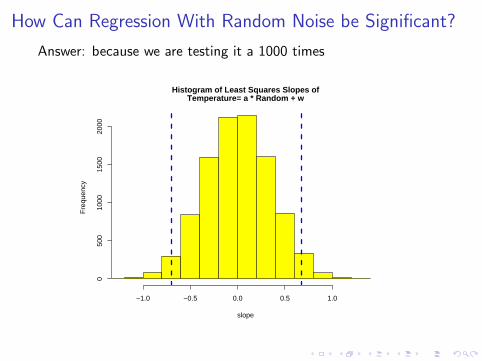
How Can Regression With Random Noise be Significant?
Answer: because we are testing it a 1000 times
slope
Fre
quen
cy
−1.0 −0.5 0.0 0.5 1.0
050
010
0015
0020
00Histogram of Least Squares Slopes of
Temperature= a * Random + w
How Can Regression With Random Noise be Significant?
I Even if true coefficient is zero, sample coefficient can be large.
I The distribution of sample coefficient is known exactly.
I The probability that sample coefficient exceeds a critical valuewhen true coefficient vanishes is the significance level.
I Histogram shows that 5% significance level is 0.68, so weexpect sample correlation to exceed 0.68 5% of the time.
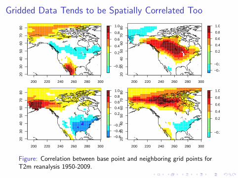
Gridded Data Tends to be Spatially Correlated Too
200 220 240 260 280 300
2030
4050
6070
80
−0.2
0.2
0.4
0.6
0.8
1.0
200 220 240 260 280 300
2030
4050
6070
80
−0.4
−0.2
0.2
0.4
0.6
0.8
1.0
200 220 240 260 280 300
2030
4050
6070
80
−0.6
−0.4
−0.2
0.2
0.4
0.6
0.8
1.0
200 220 240 260 280 300
2030
4050
6070
80
−0.2
0.2
0.4
0.6
0.8
1.0
Figure: Correlation between base point and neighboring grid points forT2m reanalysis 1950-2009.
Effect of Spatial Correlations
Correlations in space imply that if one grid point has a highcorrelation with a time series, then the neighboring points also willhave a strong correlation, no matter the true correlation.
This means that the significance tests are not independent.
We do not expect just 5% of the grid points to exceed thesignificance threshold randomly, but rather 5% of the spatiallycoherent structures to exceed the threshold.
This means that more than 5% of the area tends to exceed thesignificance threshold for spatially correlated data.
Field Significance
Field significance is the statistical significance of the hypothesisthat all regression coefficients vanish simultaneously.
To perform a field significance test, need to account for:
I multiple hypothesis are being tested simultaneously.
I variables are interdependent.
Gilbert Walker
!
! !
"#$%&'()* +$,,'+-'.* /0-1* -1'* '&'+-#$(23,'-0+* 40'&.56* 1'* )12#'.* 72(%#0.3'* 8,09'#)0-:;)*"#')-030$<)*=.2()*>#0?'*/0-1* @$)'"1*A2#($#6*/1$*%'+2('6* 0,*BCDE6*A<+2)02,*>#$4'))$#*$4*F2-1'(2-0+)G*H2&I'#*/2)*'&'+-'.*2*J'&&$/*$4*-1'*K$:2&*L$+0'-:*0,*BCDM*2,.*#'+'09'.*-1'*.'3#''*$4*L+N*4#$(*72(%#0.3'*8,09'#)0-:*-1'*)2('*:'2#G**O&0$-* #'-0#'.* $,* -1'* &2)-* .2:* $4* BCDE* 2,.*H2&I'#* -$$I* +12#3'* $4* -1'* P,.02*F'-'$#$&$30+2&*N'"2#-(',-*-1'*4$&&$/0,3*.2:G*A0I'*O&0$-*%'4$#'*10(6*1'*"#'))'.*4$#*-1'*2""$0,-(',-*$4*)+0',-040+*2))0)-2,-)G*Q'*/2)*)<++'))4<&*2,.*/'&&*#'/2#.'.6*4$#*-1'*(',*1'*+1$)'6*@GQGJ0'&.6*@G>2--'#)$,*2,.*RG7GL0(")$,6*"#$9'.*-$*%'*40#)-S+&2))*('-'$#$&$30)-)*2,.*2&&*)<%)'T<',-&:*%'+2('*.0#'+-$#)*$4*('-'$#$&$30+2&*)'#90+')*U0,*P,.026*72,2.2*2,.*-1'*8,0-'.*V0,3.$(6*#')"'+-09'&:WG*X1'*/$#I*$4*$#32,0?0,3* -1'* P,.02,* $%)'#92-$#0')* 2,.*/'2-1'#* )'#90+'* 2""'2#)* -$* 129'* -2I',* <"* 2* &$-* $4*H2&I'#;)* -0('* 2,.* ','#3:6* 4$#* 1'* "<%&0)1'.*,$-10,3*)<%)-2,-02&*4$#*)'9'#2&*:'2#)G*J#$(*-1'*$<-)'-6*1$/'9'#6*1'*-<#,'.*10)*(0,.*-$*($,)$$,*"#$%&'()6* 2)* )1$/,* %:6* 4$#* 'Y2("&'6* -1'*.$+<(',-)* 1'&.* %:* -1'* A0%#2#:* $4* 7$,3#'))*',-0-&'.*!"#$%&'"(')%)"*+,-+'",'./%')",&"",'&01)$..%-' ."'2"3%*,)%,.' $,'4#*$56'7+86' 90,%6'4020&.'+,-':%#.%)1%*';<=>6'+,-'+'?")#+*$&",'"(' ./%'("*%?+&.&'@$./'./%'+?.0+5'*+$,(+55*UP,.02*F'-'$#$&$30+2&*N'"2#-(',-6*L0(&26*BCDZWG*X1'*40#)-*$4*10)*(2,:*('-'$#$&$30+2&*"2"'#)*2""'2#'.*0,* BCDCG* O,-0-&'.* 57$##'&2-0$,* 0,* )'2)$,2&*92#02-0$,* $4* +&0(2-'56* 0-* /2)* "<%&0)1'.* 0,* -1'*A,-$+,'7%.%"*"5"2$?+5'7%)"$*&* U!"6* >2#-*[P6*\$GZ6*""GBB]SB!MWG*X1'*&'+-<#')*1'*329'*2-*-1'*8,09'#)0-:*$4*72&+<--2*0,*BCD^*/'#'*"<%&0)1'.*%:* 72(%#0.3'* 8,09'#)0-:* >#'))* 0,* BCBD* 0,* 2*9$&<('* ',-0-&'.* B0.5$,%&' "(' ./%' ./%"*8' "('%5%?.*")+2,%.$&)G* Q0)* 0,-'#')-* 0,* '&'+-#$S(23,'-0)(*-1',*2""'2#)*-$*129'*/2,'.G**Q290,3* #'+$3,0)'.* -12-* 1'* +$<&.* ,$-* -2+I&'*($,)$$,*4$#'+2)-0,3*%:*('2,)*$4*(2-1'(2-0+2&*2,2&:)0)* %2)'.* <"$,* ')-2%&0)1'.* "#'(0)')6*H2&I'#* +1$)'* 0,)-'2.* -$* <)'* '("0#0+2&*-'+1,0T<')G*N'9'&$"0,3*-1'*/$#I*$4*QGJG_&2,4$#.6*L0#*\$#(2,*A$+I:'#6*QGQGQ0&.'%#2,.))$,6*L0#*@$1,* O&0$-* 2,.* $-1'#)6* 1'* +2&+<&2-'.* )-2-0)-0+2&* &23* +$##'&2-0$,)* %'-/'',* 2,-'+'.',-*('-'$#$&$30+2&* '9',-)*/0-10,*2,.*$<-)0.'* P,.02*2,.* -1'* )<%)'T<',-*%'1290$<#*$4* -1'* P,.02,*($,)$$,* 0-)'&46* +2&&0,3* -1'* 2#-* 0,9$&9'.* 0,* <)0,3* -1'* #'&2-0$,)10")* 1'* 4$<,.* `)'2)$,2&*4$#')12.$/0,3;6* #2-1'#* -12,* 4$#'+2)-0,36* )2:0,3* -12-* 4$#')12.$/0,3* 0,.0+2-'.* 52* 923<'#*"#'.0+-0$,5*-12,*4$#'+2)-0,3G*X1$<31*10)*/$#I*/2)*&2#3'&:*)-2-0)-0+2&6*H2&I'#*2&)$*329'*-1$<31-*-$*-1'*('-'$#$&$3:*$4*-1'*2))$+02-0$,)*1'*0.',-040'.G*Q0)*/$#I*$,*-1'*\0&'*4&$$.*"#$90.')*2*+2)'*0,*"$0,-G*5P,2)(<+1*2)*-1'*\0&'*4&$$.*0)*.'-'#(0,'.*%:*-1'*($,)$$,*#20,42&&*$4*=%:))0,0256*1'*/#$-'6*52,.*2)*-1'*($0)-*/0,.)*/10+1*"#$90.'*-10)*#20,42&&*-#29'&*0,*-1'*'2#&0'#*"$#-0$,*$4*-1'0#*($9'(',-*)0.'*%:*)0.'*/0-1*-1$)'*/10+1*<&-0(2-'&:*#'2+1*-1'*,$#-1*$4*-1'*=#2%02,*L'26*-1'#'*0)*2*-$&'#2%&:*+&$)'*+$##')"$,.',+'*%'-/'',*-1'*2%<,.2,+'*$4*-1'*\0&'*4&$$.*2,.*-12-*$4*-1'*($,)$$,*#20,)*$4*,$#-1/')-*P,.025*UH2&I'#6*BCBDWG*Q'*/2)*/'&&*2/2#'*$4*-1'*&0(0-2-0$,)*$4*'("0#0+2&*)-2-0)-0+2&*('-1$.)*2,.*0,.''.6*2)*L1'""2#.*UBCaCW*"<-*0-6*5)$<31-*%:*-1'*($)-*'Y2+-0,3*('-1$.)*-$*-')-*-1'*)03,040+2,+'*$4*10)*#')<&-)5G**H2&I'#*#'-0#'.*4#$(*P,.02*0,*N'+'(%'#*BC!M*2,.*)<++''.'.*L0#*\2"0'#*L12/*2)*>#$4'))$#*$4*F'-'$#$&$3:*2-*-1'*P("'#02&*7$&&'3'*$4*L+0',+'*2,.*X'+1,$&$3:6*A$,.$,G*Q'#'6*1'*,$-*$,&:*+$,-0,<'.*10)*)-<.0')*$4*/$#&.*/'2-1'#*%<-*2&)$*)1$/'.*10()'&4*-$*%'*2*+$("'-',-*'Y"'#0(',-2&*"1:)0+0)-6* -<#,0,3* 10)* 2--',-0$,* -$* &2%$#2-$#:* )-<.0')* $4* +$,9'+-0$,* 0,* <,)-2%&'* 4&<0.)6* /0-1*"2#-0+<&2#*#'4'#',+'*-$*-1'*4$#(2-0$,*$4*+&$<.)G*X10)*/$#I*(2:*129'*%'',*)-0(<&2-'.*%:*10)*
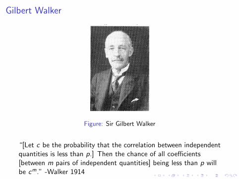
Figure: Sir Gilbert Walker
“[Let c be the probability that the correlation between independentquantities is less than p.] Then the chance of all coefficients[between m pairs of independent quantities] being less than p willbe cm.” -Walker 1914
Experimentwise Error Rate
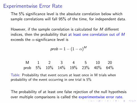
The 5% significance level is the absolute correlation below whichsample correlations will fall 95% of the time, for independent data.
However, if the sample correlation is calculated for M differentindices, then the probability that at least one correlation out of Mexceeds the α-significance level is
prob = 1− (1− α)M
M 1 2 3 4 5 10 20prob 5% 10% 14% 19% 23% 40% 64%
Table: Probability that event occurs at least once in M trials whenprobability of the event occurring in one trial is 5%
The probability of at least one false rejection of the null hypothesisover multiple comparisons is called the experimentwise error rate.
Multiple Comparisons
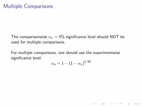
The comparisonwise αc = 5% significance level should NOT beused for multiple comparisons.
For multiple comparisons, one should use the experimentwisesignificance level:
αe = 1− (1− αc)1/M
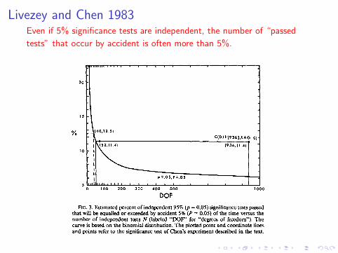
Livezey and Chen 1983Even if 5% significance tests are independent, the number of “passed
tests” that occur by accident is often more than 5%.
Effect of Spatial Correlations
Large cross-correlations in the field reduce the “degreesof freedom” in the field. -Livezey and Chen 1983
The “effective” number of degrees of freedom is not known, butcan be estimated by a variety of techniques.
Monte Carlo Estimate of Field Significance
Livezey and Chen (1983) procedure:
I Replace pre-specified time series with random numbers drawnfrom same distribution as pre-specified time series.
I Calculate correlation maps between field and random numbers.
I Count the number of “passed tests” in the field.
I Repeat many times and record the counts.
I Compare observed count with counts from random numbers.
I If observed count falls in the upper 5th percentile, rejecthypothesis that all correlation vanish.
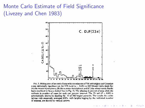
Monte Carlo Estimate of Field Significance(Livezey and Chen 1983)
Limitations of “Counting” Methods
Counting methods count the number of passed testsregardless of spatial location or degree of significance.
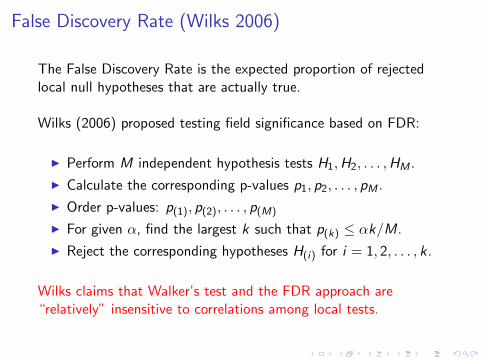
False Discovery Rate (Wilks 2006)
The False Discovery Rate is the expected proportion of rejectedlocal null hypotheses that are actually true.
Wilks (2006) proposed testing field significance based on FDR:
I Perform M independent hypothesis tests H1,H2, . . . ,HM .
I Calculate the corresponding p-values p1, p2, . . . , pM .
I Order p-values: p(1), p(2), . . . , p(M)
I For given α, find the largest k such that p(k) ≤ αk/M.
I Reject the corresponding hypotheses H(i) for i = 1, 2, . . . , k .
Wilks claims that Walker’s test and the FDR approach are“relatively” insensitive to correlations among local tests.
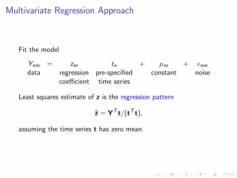
Multivariate Regression Approach
Fit the model
Ynm = zm tn + µm + εnm
data regression pre-specified constant noisecoefficient time series
Least squares estimate of z is the regression pattern
z = YT t/(tT t),
assuming the time series t has zero mean.
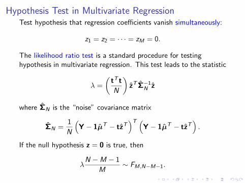
Hypothesis Test in Multivariate RegressionTest hypothesis that regression coefficients vanish simultaneously:
z1 = z2 = · · · = zM = 0.
The likelihood ratio test is a standard procedure for testinghypothesis in multivariate regression. This test leads to the statistic
λ =
(tT t
N
)zT Σ−1
N z
where ΣN is the “noise” covariance matrix
ΣN =1
N
(Y − 1µT − tzT
)T (Y − 1µT − tzT
).
If the null hypothesis z = 0 is true, then
λN −M − 1
M∼ FM,N−M−1.
Problem With Multivariate Hypothesis Test
In typical climates studies, noise covariance matrix ΣN is singularbecause the number of coefficients exceeds the sample size.
This means the regression problem is underdetermined.
Discriminant Analysis Approach
Find the linear combination of variables that maximizes thefraction of variance explained by the pre-specified time series.
Equivalently, find the linear combination of variables thatmaximizes the correlation with the pre-specified time series.
Discriminant Analysis Approach
Let weights be qm. Then linear combination gives the time series
rn =∑m
Ynmqm.
Fit the time series to the pre-specified time series:
rn = αtn + εn.
The fraction of variance explained by the pre-specified time series is
“Signal-to-noise ratio” = STR =var[αtn]
var[rn]
We seek weights q that maximizes the signal-to-total ratio STR.
Solution to Discriminant Analysis
The weights that maximize STR can be found analytically as
q = Σ−1N z.
The signal-to-noise ratio (SNR) turns out to be
SNR = λ =
(tT t
N
)zT Σ−1
N z.
Discriminant analysis and multivariate analysis lead to the same λ.
Discriminant analysis shows that λ is the optimal signal-to-noiseratio of a linear combination of variables.
Significance test for SNR is exactly the same as the significancetest of z = 0 in multivariate regression.
Limitation of Discriminant Analysis
Exactly the same as multivariate regression: ΣN is singular.

Practical Approach
I Transform data into principal components.
I Select a small number of PCs to represent the data.
I Solve regression and discriminant problems in PC-space.
I Transform solutions back into data space.
Example: Trend Analysis
I Annual mean sea surface temperature (SST) 1948-2009.
I Data from ERSSTv3b, Smith and Reynolds (2004).
I 2◦ × 2◦ grid.
I t is a linear function of year, incrementing by 1/10.
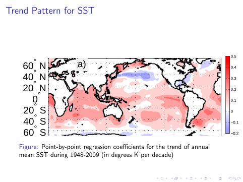
Trend Pattern for SST
a)
60° S 40° S 20° S
0° 20° N 40° N 60° N
b)
60° S 40° S 20° S
0° 20° N 40° N 60° N
c)
60° S 40° S 20° S
0° 20° N 40° N 60° N
−0.2
−0.1
0
0.1
0.2
0.3
0.4
0.5
d)
0° 60° E 120° E 180° E 120° W 60° W 60° S 40° S 20° S
0° 20° N 40° N 60° N
0
10
20x 10
−4
a)
60° S 40° S 20° S
0° 20° N 40° N 60° N
b)
60° S 40° S 20° S
0° 20° N 40° N 60° N
c)
60° S 40° S 20° S
0° 20° N 40° N 60° N
−0.2
−0.1
0
0.1
0.2
0.3
0.4
0.5
d)
0° 60° E 120° E 180° E 120° W 60° W 60° S 40° S 20° S
0° 20° N 40° N 60° N
0
10
20x 10
−4
Figure: Point-by-point regression coefficients for the trend of annualmean SST during 1948-2009 (in degrees K per decade)
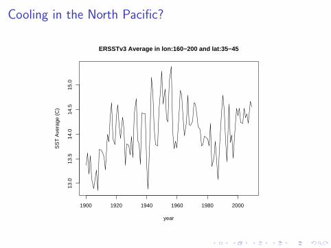
Cooling in the North Pacific?
1900 1920 1940 1960 1980 2000
13.0
13.5
14.0
14.5
15.0
year
SS
T A
vera
ge (
C)
ERSSTv3 Average in lon:160−200 and lat:35−45
Discriminant Analysis
5 10 15 20 25 30 35 400
0.5
1S
TR
a)
5 10 15 20 25 30 35 400
0.2
0.4
CV
MS
E
b)
5 10 15 20 25 30 35 40−0.4
−0.2
0
0.2
PC
Slo
pe (
per
10yr
) c)
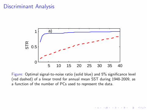
Figure: Optimal signal-to-noise ratio (solid blue) and 5% significance level(red dashed) of a linear trend for annual mean SST during 1948-2009, asa function of the number of PCs used to represent the data.
Comments About Discriminant Analysis Results
I The STR is statistically significant at all PC truncations.
I Most of the STR arises from the first three PCs.
I Little gain in STR using more than three PCs.
How Many PCs Should Be Chosen?
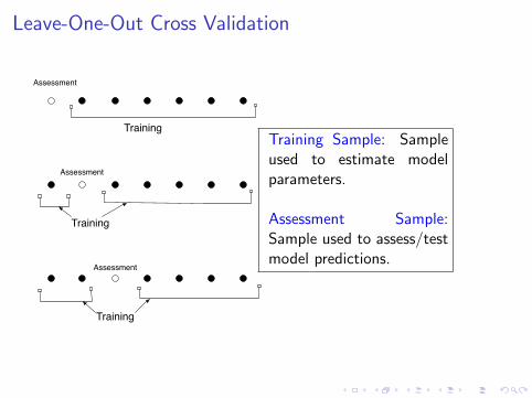
Leave-One-Out Cross Validation
Training
Training
Training
Assessment
Assessment
Assessment
Training Sample: Sampleused to estimate modelparameters.
Assessment Sample:Sample used to assess/testmodel predictions.
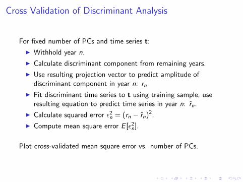
Cross Validation of Discriminant Analysis
For fixed number of PCs and time series t:
I Withhold year n.
I Calculate discriminant component from remaining years.
I Use resulting projection vector to predict amplitude ofdiscriminant component in year n: rn
I Fit discriminant time series to t using training sample, useresulting equation to predict time series in year n: rn.
I Calculate squared error ε2n = (rn − rn)2.
I Compute mean square error E [ε2n].
Plot cross-validated mean square error vs. number of PCs.
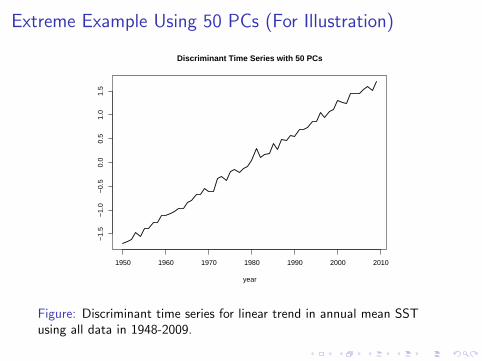
Extreme Example Using 50 PCs (For Illustration)
1950 1960 1970 1980 1990 2000 2010
−1.
5−
1.0
−0.
50.
00.
51.
01.
5
year
Discriminant Time Series with 50 PCs
Figure: Discriminant time series for linear trend in annual mean SSTusing all data in 1948-2009.
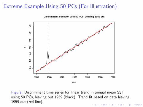
Extreme Example Using 50 PCs (For Illustration)
1950 1960 1970 1980 1990 2000 2010
−1.
5−
1.0
−0.
50.
00.
51.
01.
5
year
r
1950 1960 1970 1980 1990 2000 2010
−1.
5−
1.0
−0.
50.
00.
51.
01.
5
Discriminant Function with 50 PCs, Leaving 1959 out
Figure: Discriminant time series for linear trend in annual mean SSTusing 50 PCs, leaving out 1959 (black). Trend fit based on data leaving1959 out (red line).
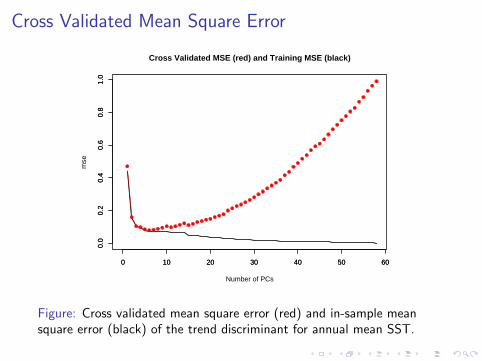
Cross Validated Mean Square Error
0 10 20 30 40 50 60
0.0
0.2
0.4
0.6
0.8
1.0
Number of PCs
mse
0 10 20 30 40 50 60
0.0
0.2
0.4
0.6
0.8
1.0
Cross Validated MSE (red) and Training MSE (black)
Figure: Cross validated mean square error (red) and in-sample meansquare error (black) of the trend discriminant for annual mean SST.
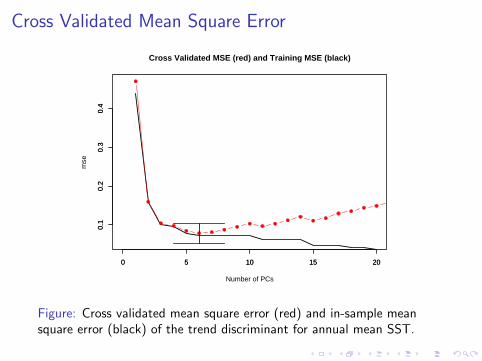
Cross Validated Mean Square Error
0 5 10 15 20
0.1
0.2
0.3
0.4
Number of PCs
mse
0 5 10 15 20
0.1
0.2
0.3
0.4
Cross Validated MSE (red) and Training MSE (black)
Figure: Cross validated mean square error (red) and in-sample meansquare error (black) of the trend discriminant for annual mean SST.
Trend Discriminant for SST
a)
60° S 40° S 20° S
0° 20° N 40° N 60° N
b)
60° S 40° S 20° S
0° 20° N 40° N 60° N
c)
60° S 40° S 20° S
0° 20° N 40° N 60° N
−0.2
−0.1
0
0.1
0.2
0.3
0.4
0.5
d)
0° 60° E 120° E 180° E 120° W 60° W 60° S 40° S 20° S
0° 20° N 40° N 60° N
0
10
20x 10
−4
a)
60° S 40° S 20° S
0° 20° N 40° N 60° N
b)
60° S 40° S 20° S
0° 20° N 40° N 60° N
c)
60° S 40° S 20° S
0° 20° N 40° N 60° N
−0.2
−0.1
0
0.1
0.2
0.3
0.4
0.5
d)
0° 60° E 120° E 180° E 120° W 60° W 60° S 40° S 20° S
0° 20° N 40° N 60° N
0
10
20x 10
−4
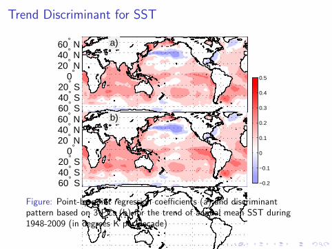
Figure: Point-by-point regression coefficients (a) and discriminantpattern based on 3 PCs (b) for the trend of annual mean SST during1948-2009 (in degrees K per decade)
Comparison With EOF
a)
60° S 40° S 20° S
0° 20° N 40° N 60° N
b)
60° S 40° S 20° S
0° 20° N 40° N 60° N
c)
60° S 40° S 20° S
0° 20° N 40° N 60° N
−0.2
−0.1
0
0.1
0.2
0.3
0.4
0.5
d)
0° 60° E 120° E 180° E 120° W 60° W 60° S 40° S 20° S
0° 20° N 40° N 60° N
0
10
20x 10
−4
a)
60° S 40° S 20° S
0° 20° N 40° N 60° N
b)
60° S 40° S 20° S
0° 20° N 40° N 60° N
c)
60° S 40° S 20° S
0° 20° N 40° N 60° N
−0.2
−0.1
0
0.1
0.2
0.3
0.4
0.5
d)
0° 60° E 120° E 180° E 120° W 60° W 60° S 40° S 20° S
0° 20° N 40° N 60° N
0
10
20x 10
−4
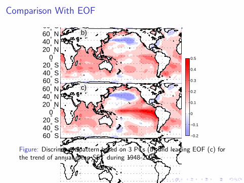
Figure: Discriminant pattern based on 3 PCs (b) and leading EOF (c) forthe trend of annual mean SST during 1948-2009.
Discriminant Projection Pattern for SSTa)
60° S 40° S 20° S
0° 20° N 40° N 60° N
b)
60° S 40° S 20° S
0° 20° N 40° N 60° N
c)
60° S 40° S 20° S
0° 20° N 40° N 60° N
−0.2
−0.1
0
0.1
0.2
0.3
0.4
0.5
d)
0° 60° E 120° E 180° E 120° W 60° W 60° S 40° S 20° S
0° 20° N 40° N 60° N
0
10
20x 10
−4
a)
60° S 40° S 20° S
0° 20° N 40° N 60° N
b)
60° S 40° S 20° S
0° 20° N 40° N 60° N
c)
60° S 40° S 20° S
0° 20° N 40° N 60° N
−0.2
−0.1
0
0.1
0.2
0.3
0.4
0.5
d)
0° 60° E 120° E 180° E 120° W 60° W 60° S 40° S 20° S
0° 20° N 40° N 60° N
0
10
20x 10
−4
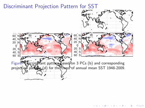
Figure: Discriminant pattern based on 3 PCs (b) and correspondingprojection pattern (d) for the trend of annual mean SST 1948-2009.
Time Series for Discriminant and Principal Component
Year
a)
1950 1960 1970 1980 1990 2000
−2
0
2
Year
b)
1950 1960 1970 1980 1990 2000
−2
0
2
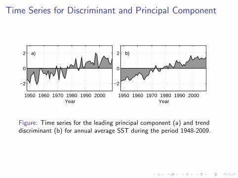
Figure: Time series for the leading principal component (a) and trenddiscriminant (b) for annual average SST during the period 1948-2009.
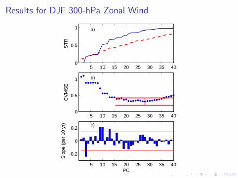
Results for DJF 300-hPa Zonal Wind
5 10 15 20 25 30 35 400
0.5
1
ST
R
a)
5 10 15 20 25 30 35 400
0.5
1
CV
MS
E
b)
5 10 15 20 25 30 35 40
−0.2
0
0.2
PC
Slo
pe (
per
10 y
r) c)
Results for DJF 300-hPa Zonal Wind
0°
20° N
40° N
60° N
80° N
1010 10
1010
10
10
30
3030 30
a)
101010 10
1010
10
10
10
30 30
3030 30
b)
0°
20° N
40° N
60° N
80° N
101010 10
1010
10
10
10
30 30
3030 30
c)
0°
20° N
40° N
60° N
80° N
−3
−2
−1
0
1
2
3
d)
0° 60° E 120° E 180° E 120° W 60° W 0°
20° N
40° N
60° N
80° N
−5
0
5x 10
−4
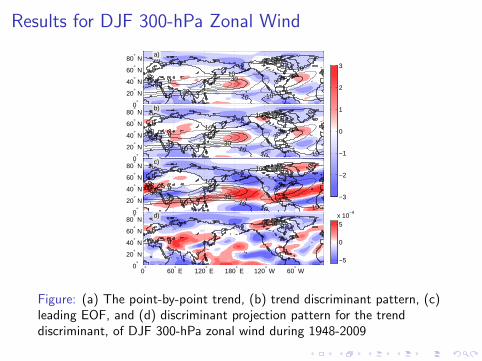
Figure: (a) The point-by-point trend, (b) trend discriminant pattern, (c)leading EOF, and (d) discriminant projection pattern for the trenddiscriminant, of DJF 300-hPa zonal wind during 1948-2009
Results for DJF 300-hPa Zonal Wind
1010
1010
3030 30
0° 60° E 120° E 180° E 120° W 60° W 0°
20° N
40° N
60° N
80° N
0
5
10
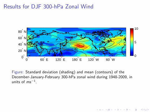
Figure: Standard deviation (shading) and mean (contours) of theDecember-January-February 300-hPa zonal wind during 1948-2009, inunits of ms−1.
Results for DJF 300-hPa Zonal Wind
Year
a)
1950 1960 1970 1980 1990 2000
−2
0
2
Year
b)
1950 1960 1970 1980 1990 2000
−2
0
2
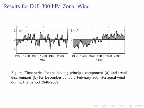
Figure: Time series for the leading principal component (a) and trenddiscriminant (b) for December-January-February 300-hPa zonal windduring the period 1948-2009.
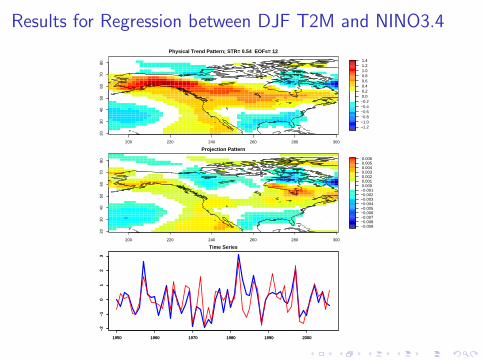
Results for Regression between DJF T2M and NINO3.4
200 220 240 260 280 300
2030
4050
6070
80
−1.2−1.0−0.8−0.6−0.4−0.2 0.0 0.2 0.4 0.6 0.8 1.0 1.2 1.4
Physical Trend Pattern; STR= 0.54 EOFs= 12
200 220 240 260 280 300
2030
4050
6070
80
−0.009−0.008−0.007−0.006−0.005−0.004−0.003−0.002−0.001 0.000 0.001 0.002 0.003 0.004 0.005 0.006
Projection Pattern
1950 1960 1970 1980 1990 2000
−2
−1
01
23
Time Series
1950 1960 1970 1980 1990 2000
−2
−1
01
23
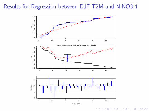
Results for Regression between DJF T2M and NINO3.4
0 10 20 30 40 50
0.0
0.2
0.4
0.6
0.8
1.0
ST
R
0 10 20 30 40 50
0.0
0.2
0.4
0.6
0.8
1.0
0 10 20 30 40 50
0.0
0.2
0.4
0.6
0.8
1.0
mse
0 10 20 30 40 50
0.0
0.2
0.4
0.6
0.8
1.0
Cross Validated MSE (red) and Training MSE (black)
0 10 20 30 40 50
−0.
4−
0.2
0.0
0.2
Number of PCs
Slo
pe o
f PC
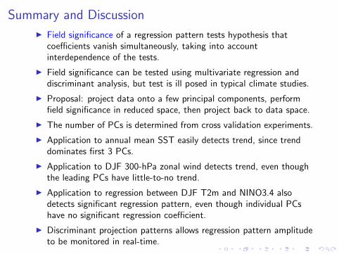
Summary and Discussion
I Field significance of a regression pattern tests hypothesis thatcoefficients vanish simultaneously, taking into accountinterdependence of the tests.
I Field significance can be tested using multivariate regression anddiscriminant analysis, but test is ill posed in typical climate studies.
I Proposal: project data onto a few principal components, performfield significance in reduced space, then project back to data space.
I The number of PCs is determined from cross validation experiments.
I Application to annual mean SST easily detects trend, since trenddominates first 3 PCs.
I Application to DJF 300-hPa zonal wind detects trend, even thoughthe leading PCs have little-to-no trend.
I Application to regression between DJF T2m and NINO3.4 alsodetects significant regression pattern, even though individual PCshave no significant regression coefficient.
I Discriminant projection patterns allows regression pattern amplitudeto be monitored in real-time.