Distributed Multivariate Regression Using Wavelet-based Collective

Distributed Multivariate Regression UsingWavelet-based Collective Data Mining.

Daryl E. Hershberger and Hillol KarguptaSchool of Electrical Engineering and Computer Science, Washington State University

Pullman, Washington 99164-2752, USA

E-mail: dhershbe and hillol @eecs.wsu.edu

This paper presents a method for distributed multivariate regression using wavelet-

based Collective Data Mining (CDM). The method seamlessly blends machine

learning and the theory of communication with the statistical methods employed

in parametric multivariate regression to provide an effective data mining technique

for use in a distributed data and computation environment. The technique is ap-

plied to two benchmark data sets, producing results that are consistent with those

obtained by applying standard parametric regression techniques to centralized data

sets. Evaluation of the method in terms of model accuracy as a function of appropri-

ateness of the selected wavelet function, relative number of non-linear cross-terms,

and sample size demonstrates that accurate parametric multivariate regression mod-

els can be generated from distributed, heterogeneous, data sets with minimal data

communication overhead compared to that required to aggregate a distributed data

set. Application of this method to Linear Discriminant Analysis, which is related

to parametric multivariate regression, produced classification results on the Iris data

set that are comparable to those obtained with centralized data analysis.

Key Words: data mining, distributed data mining, collective data mining, knowledge discovery,

wavelets, regression

1. INTRODUCTION

This paper presents an approach to distributed multivariate regression using wavelet-based Collective Data Mining (CDM) [25]. CDM is an approach to Distributed DataMining (DDM) that addresses difficulties introduced when distributed data sites observeheterogeneous sets of features.

Distributed data mining deals with methods of finding data patterns in a distributed dataand computation environment. DDM methods allow distributed data to be analyzed withminimal data communication. Generally, DDM algorithms start with local data analysisfollowed by generation of a global model based on combining the results of the localanalysis. In the general case, where different sites observe different sets of features, naiveapproaches to local analysis may be ambiguous and incorrect, resulting in incorrect global

1

2 ! Please write�� ! �"�#�$

in file !

models. CDM provides a well-grounded methodology to address this general case, offeringan approach to the analysis of distributed, heterogeneous databases with distinct featurespaces.

The foundation of CDM is the observation that any function may be represented indistributed fashion by using an appropriate set of basis functions. Communication theoryprovides that efficient transmission of information is facilitated through the use of orthogo-nal functions [17]. Wavelet analysis techniques [37] provide a powerful tool for generatingorthogonal basis function sets for use in CDM.

Parametric Multivariate Regression (MR) is a widely used statistical data analysis tech-nique that can also be viewed as a supervised learning algorithm. The distributed MRtechnique presented here learns local information in terms of the coefficients of an orthog-onal basis function representation, transmits a small (relative to the sample size) number ofsignificant coefficients to a central site, and then generates a global model directly from thatsmall set of significant coefficients. The method seamlessly blends machine learning andthe theory of communication with the statistical methods employed in MR to provide aneffective data mining technique for use in a distributed data and computation environment.

Section 2 begins with a description of the general DDM problem of heterogeneous datasets. This is followed by a review of related DDM work and an overview of MR. Thesection concludes with an example of the specific problem of naive data analysis withinthe context of parametric regression models in a DDM environment. Section 3 provides anoverview of the foundations of CDM and a description of the wavelet techniques used forthe distributed MR model. An algorithm for distributed MR using wavelet-based CDM ispresented in Section 4. The performance of this CDM-MR method is then characterizedusing real “benchmark” data sets and larger synthetic data sets. Section 5 describes theapplication of the CDM regression model to Linear Discriminant Analysis (LDA) whichis related to parametric multivariate regression. Section 6 summarizes the CDM workpresented here for MR models and LDA, and discusses future research directions.

2. BACKGROUND

This section presents background material related to MR models using wavelet-basedCDM. A simple model of distributed, heterogeneous, data sites is explained first. This isfollowed by a review of related DDM research. Next a brief overview of MR is providedand finally an example that demonstrates the incorrect results that may be obtained by naiveapplication of parametric regression techniques to distributed data is presented.

f x x 21

-7.0

-9.5

4.3

-4.2

-9.0

-2.5

3.4

6.7

-4.9

-1.3

3.4

-6.9

-8.7

9.8

3.8

f x 5 x 6 x

5.1

7

-7.0

-9.5

4.3

-4.2

-9.0

-4.0

-1.7

1.8

-9.9

3.9 7.9 2.7

6.2

7.1

-3.5

-6.5 0.8

8.6

8.7

4.9

Site A Site B Site C

x 2

3.4

-6.9

-8.7

9.8

3.8

x 3 x 4

-8.7

-3.5

-5.7

-8.0

0.1 -7.4

7.7

9.9

-2.7

FIG. 1. Distributed data sites with a vertically partitioned feature space.

! Please write�� " �� #�$

in file ! 3

2.1. MotivationDDM deals with the problem of finding data patterns in an environment with distributed

data and computation. A typical application domain of DDM either has inherently dis-tributed data sources or centralized data partitioned at different sites. The data sites may behomogeneous, i.e. each site stores data for exactly the same set of features. In the generalcase, however, the data sites may be heterogeneous, each site maintaining databases withdifferent kinds of information. For example, financial institutions (banks, insurance com-panies, credit-card issuers) wish to combat fraud and posses data that would be of use toone another in this effort. However, customer privacy concerns prevent this data from beingcombined into a single data base. CDM allows pertinent information and data patterns to beextracted from the individual data bases without compromising customer privacy. Anotherexample of distributed heterogeneous data sets is the local data associated with a large setof distributed sensors (either environmental or industrial) where the sensed parameters aredifferent. There may be no organizational barriers to centralizing this data but time andprocessing constraints may give CDM an advantage over centralized techniques.

In the general case the feature sets observed at different sites are different. A simpleexample of this is the case of a vertically partitioned data set. Figure 1 illustrates thissituation. While this paper considers the problem of developing MR models for thissimple case of vertically partitioned data sets, CDM is applicable to the general case ofheterogenous data sets and it is expected that CDM-MR may be extended to this generalcase.

Given a set of observations representing discretely sampled continuous valued features,the task is to use parametric regression techniques to learn a function that estimates theunknown value of a dependent feature as a function of other observed independent features.The given set of observed feature values is sometimes called the training data set. In Figure1 the column for

�denotes the feature value to be estimated; �� and ��

denote the independent features that are used to estimate�

. The data sets available at thedifferent sites are used as the data that the regression is performed on. If the

�column is

not observed everywhere and it is required to learn the local models it is broadcasted toevery site.

One requirement for implementation of DDM algorithms with vertically partitioned datasets is a method for properly aligning the feature pattern vectors in different partitions witheach other. This requirement introduces a certain amount of flexibility in defining relationsamong feature sets. One possibility is to use an operation similar to the Join operation ofrelational data bases. Note that in Figure 1 site A and B share feature � � while site A andC share feature

�. The alignment of the feature pattern vectors at sites A and B could be

accomplished by a Join based on � � followed by alignment with the pattern vectors at siteC using Join based on

�. If no common feature exists then an association must be made

based on some prior knowledge or expectation regarding the model under development.As Figure 1 shows each site may observe features such that a majority are unique to

that site and therefore the sites are called heterogeneous. There exists little work for thisgeneral case of DDM. The following section reviews related work in DDM.

2.2. Related WorkThis section briefly reviews some of the existing DDM work. This work may be

grouped into four basic categories, Meta-learning and Stacking, Collective Data Mining,


in file !

Distributed Association Rule Learning,and other DDM techniques. Following these severalexperimental DDM systems are reviewed.

Meta-learning [6, 5, 7] and Stacking [38] are examples of techniques for mining homo-geneous distributed data. In the meta-learning approach supervised learning techniques arefirst used to detect concepts at local data sites, then meta-level concepts are learned froma data set generated using the locally learned concepts, resulting in a meta-classifier. Dif-ferent inductive learning algorithms may be employed to learn the local concepts, and themeta-level learning may be applied recursively, producing a hierarchy of meta-classifiers.The JAM system [33] is a meta-learning base distributed data mining framework that hasbeen used for fraud detection in the banking domain [28].

Collective data mining [24, 25] address the issues associated with mining heterogeneousdata sites. At the foundation of CDM is the observation that any function may be representedin a distributed manner using an appropriate set of basis functions. By using orthogonalbasis function, correct models of local information may be developed in terms of the basisfunction coefficients. A global model may be generated by communicating a small fractionof the local basis coefficients to a central site. Learning algorithms that have been applied toCDM include decision trees and the parametric multivariate regression techniques presentedin this paper.

The mining of association rules in distributed data bases has been examined in [9]. Inthis work the Distributed Mining of Association rules (DMA) algorithm is presented. Thisalgorithm takes advantage of the inherent parallel environment of a distributed database asopposed to previous works that tended to be sequential in nature.

The fragmented approach to mining classifiers from distributed data sources is suggestedby [10]. In this method a single, best, rule is generated in each distributed data source.These rules are then ranked using some criterion and some number of the top ranked rulesare selected to form the rule set. In [27] the authors extend efforts to automatically producea Bayesian belief network from discovered knowledge by developing a distributed approachto this exponential time problem.

In [39] the author presents two models of distributed Bayesian learning. Both modelsemploy distributed agent learners each of which observes a sequence of examples andproduces an estimate of the parameter specifying the target distribution and a populationlearner that combines the output of the agent learners in order to produce a significantlybetter estimate of the parameter of the target distribution. One model applies to situationsin which the agent learners observe data sequences generated according to the identicaltarget distribution while the second model applies when the data sequences may not havethe identical target distribution over all agent learners.

The PADMA system [23, 22] achieves scalability by locating agents with the distributeddata sources. An agent coordinating facilitator gives user requests to local agents that thenaccess and analyze local data, returning analysis results to the facilitator which mergesthe results. The high level results returned by the local agents are much smaller than theoriginal data thus allowing economical communication and enhancing scalability. Theauthors report on a PADMA implementation for unstructured text mining but note that thearchitecture is not domain specific.

Papyrus, a system in development by the National Center for Data Mining [16], is ahierarchical organization of the nodes within a data mining framework. The intent of thisproject is to develop a distributed data mining system that reflects the current distribution


in file ! 5

of the data across multiple sites and the existing network configurations connecting theseconfigurations.

Another system under development [36] concerns itself with the efficient decompositionof the problem in a distributed manner and utilizes clustering and Expected Maximizationalgorithms for knowledge extraction.

Work has also been done concerning using the Internet [8] as the framework for largescale data mining operations. This work is also applicable to intra-nets, and addressesissues of heterogeneous platforms and security issues.

The WoRLD system [1] for inductive rule-learning from multiple distributed databasesuses spreading activation instead of item-by-item matching as the basic operation of theinductive engine. Database items are labeled with markers ( indicating in or out of concept)that are then propagated through databases looking for values where in or out of conceptmarkers accumulate.

A basic requirement of algorithms employed in DDM is that they have the ability to scaleup. A survey of methods of scaling up inductive learning algorithms is presented in [32].

2.3. Overview of Multivariate RegressionMR is a widely used data analysis technique owing to its ease of use and intuitive

theoretical basis [30, 13]. MR involves fitting a parametric function model to a set of data.In this sense it is a form of inductive supervised learning.

The functions analyzed have the form� �� where the �� -s are

constant coefficients and the � � terms are linear or non-linear functions of the feature set.For example, if the feature set contains features �� and �� , then �� , � � � , and ��

�may

be present in the � � terms of the function.Given a data set consisting of samples values of the features in the feature set and the

associated function value, possibly containing some random error, the objective of MR isto produce an estimate !� � !� � �"!� � � � �#��$�"!� � � � of the function

�where the regression

model coefficients !�� are estimates of the �� . The technique used in MR is to find the set

of !� � -s that minimize %�&'� �)( !� � � , the sum of the squares of the difference between thesample and estimated function value over the data sample set.

Using matrix notation to represent the function relation in terms of a data set of size *gives

+ �,)- �/.where

+is a *1032 matrix of function sample values, , is a *10"4 matrix where each

column represents the sample data for one independent feature or regressor and each rowcontains the set of observed values of the independent features for one sample, - is a 450)2matrix of the � � -s, and . is a *60/2 matrix of values representing errors in the measuredvalue of

�. If the matrix ,87�, is invertible then the minimum squared error estimate of

the regression coefficients is

9-:� � , 7 , ��;=< , 7 +

where9- is a 4)0"2 matrix of !�>� -s.

The following section provides an example of the problems that may arise from naiveapplication of MR to vertically partitioned data sets.


in file !

02

46

810-10

-8-6-4-20

0102030

02

46

810

2 4 6 8 10

222426283032

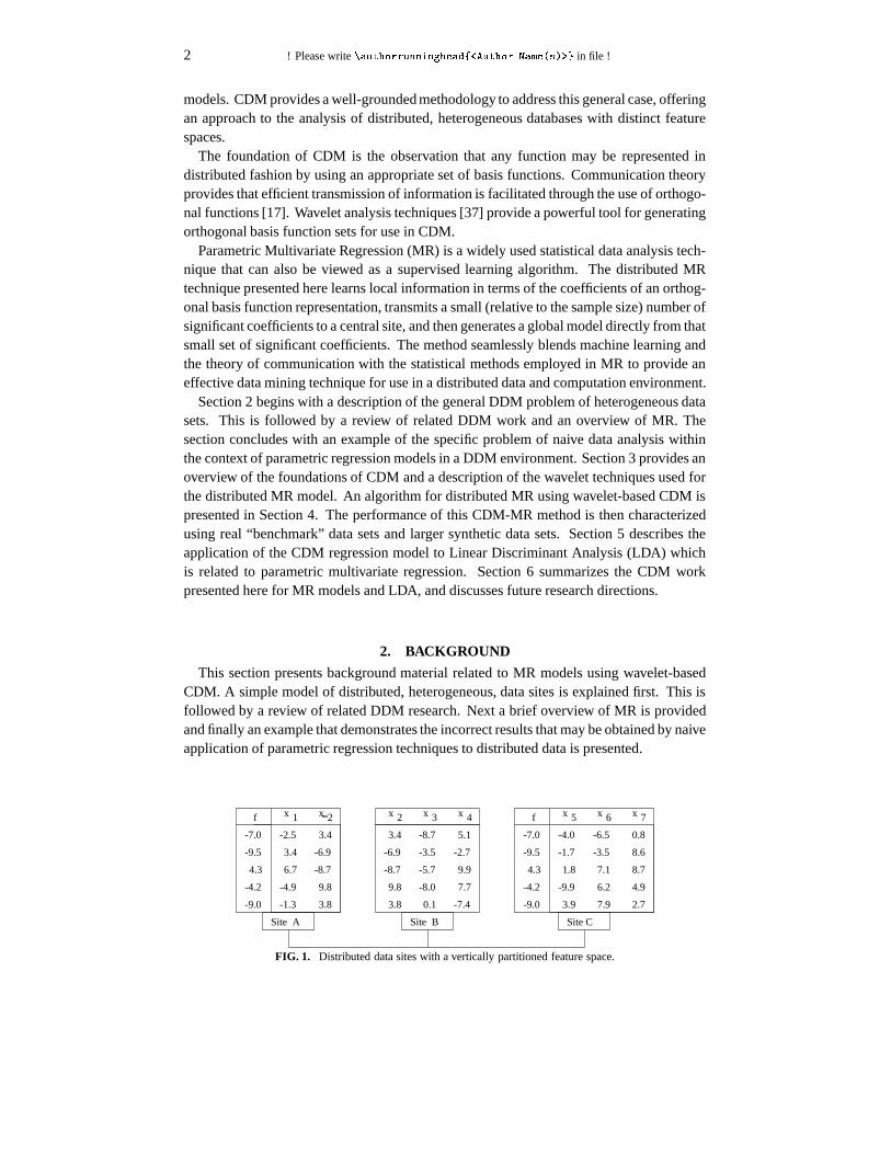
FIG. 2. (Left) The global error function. (Right) The local error function at site A.

2.4. The Naive Approach to Local Regression ModelsData modeling is a mature field that has many well-understood techniques in its ar-

senal, including parametric regression. However, like many of these traditional tech-niques, parametric regression cannot be directly used in a distributed environment witha vertically partitioned feature space. The following example demonstrates that even asimple decomposable parametric regression problem with no measurement error can pro-duce misleading results in a distributed environment. Consider the function, � � � � � � � �� ( �

�� , where � and �� are real valued variables, and the sample data set �� $2� � ��2� � �� ( � �� ( � �� ( 2 � �� ( 2 � �� ( � �� , where each entryis of the form �� $� . Let us try to fit a model, !� �� !� � �"!� � � � , to thisdata by minimizing the mean-square error. The overall mean square error computed over thedata set is, � % � �� & �

� ( !� � � � � � � � � ( !� � � �� ( � ( !� � � � �� ( !� � � ( � ( !� � �Figure 2 (Left) shows the error surface with a global minima at !� � �

and !� � � ( �. It is

a simple quadratic function and finding the minima is quite straight forward.Now let us consider the data set to be vertically partitioned; meaning � is observed at

site A and � � is observed at a different site, B. Let us choose a linear model !� �� !� � .The mean square error function for site A is

� % � � � � � � & ��"( !� � � � � � � � � ( !� � � �

�� ( 2� � � ( !� � . Figure 2 (Right) shows this local error function. It clearly shows thatthe minima of this error function is not the same as the globally optimal value of !� , i.e. 5.This example demonstrates that even for simple linear data and models naive approachesto minimize mean-square error may be misleading in a distributed environment. As willbe demonstrated later in this paper, wavelet-based CDM offers a correct, viable solution tothis problem.

3. COLLECTIVE DATA MINING AND WAVELET BASIS

This section provides an overview of the foundations of CDM and the wavelet basis usedfor the distributed MR model developed later.


in file ! 7

3.1. The Foundations of Collective Data MiningA thorough treatment of the foundations of CDM is presented in Kargupta et. al. [25].

What follows in this section is an abbreviated summary of that work as it applies todistributed MR.

In MR relations among the different members of the domain and the correspondingmembers in the range (class labels or the output function values, denoted by

�) are

desired. The goal is to learn a function !�� from the data set � � �� generated by an underlying function

�� such that the !� approximates

�. Individual members of the domain � � � �� are�

-tuples and the �� -s correspond to individual features of the domain.The foundation of CDM is based on the fact that by using an appropriate set of basis

functions any function can be represented in a distributed fashion. Let � be a possiblyinfinite set of basis functions. Associate an index with each basis function in � and denotethe 4 -th basis function in � by � and the set of all such indices of the basis functions as�"! . The function

� �� can be represented as

� �� $#��&%('

) � � �� (1)

where ) � denotes the coefficient of the 4 -th basis function. The objective is to generate afunction !� �� that approximates

� �� from a given data set

!� �� $#��*%('

!) � � �� (2)

where !� ! denotes a subset of � ! and !) � denotes the approximate estimation of thecoefficients ) � . For distributed MR using wavelet-based CDM the underlying task isessentially to compute the significant wavelet coefficients, !) � -s.

If a function has a large number of significant basis coefficients exponential time (innumber of features) is required for computing the orthonormal representation. In orderto have polynomial time computation of the coefficients, two conditions must be met:1) a sparse representation where most of the coefficients are zero or negligible, and 2)approximate evaluation of the significant coefficients.

In most MR models non-linearity typically remains bounded so not all the featuresnon-linearly interact with every other feature. It is normally acceptable to assume that thenumber of features that non-linearly interact with any given feature is bounded by someconstant. If this is not true then the problem is completely non-linear and is likely to bedifficult for even a centralized data mining algorithm let alone DDM. This requirementhas a deep root in issues of polynomial time, probabilistic and approximate learn-ability[26]. Bounded non-linearity assures that the orthonormal representation will be sparse,satisfying the first condition of polynomial time computation.

The second condition is associated with the fact that only a sample from the domainwill be available for computing the basis coefficients. This will not cause a problem aslong as our sample size is reasonable. To illustrate the rationale behind this observationconsider what happens when both sides of Equation 1 are multiplied by ,+ �� resultingin

� �� -+ �� % ��&% '/.

� � �� -+ �� . If the sample data set is denoted by , then by


in file !

summing both side over all members of the result is

#�� &

� �� -+ �� #�� &

#��&% ' .

� � �� -+ �� (3)

Since -+�� -+ �� 2 then % �� & -+ �� -+ �� where

� � is the sample size andit follows that

2� �#�� &

� �� -+ �� . + �#�

�&% ' � �� + .� % �� & � ��

� -+ ��

If the population mean over the complete domain is zero then the sample mean mustapproach zero as the sample size increases. Since � & � % �� &

� �� -+�� is the samplemean it follows that for large sample sizes (typically the case for data mining problems)the last term should approach zero.

In summary the primary steps of the CDM algorithm are [21]

1. generate appropriate orthonormal basis coefficients at each local site;2. if needed, move an appropriately chosen sample of the data sets from each site to

a single site and generate the approximate basis coefficients corresponding to non-linearcross terms;

3. combine the local models, transform the model into the user described canonicalrepresentation, and output the model.

It should be noted that the approach to distributed MR using wavelet-based CDM does notrequire the transfer of raw data (feature sample values) to a central site in order to estimatenon-linear cross terms. These estimates are instead generated directly from the local modelorthonormal basis coefficients.

The following section introduces the wavelet methods [37] used to create the orthonormalbasis representation needed for implementing distributed MR in CDM.

3.2. Wavelet Basis and Wavelet-Packet AnalysisA wavelet basis consists of a set of scaling basis functions � � and a set of wavelet basis

functions � � . The wavelet functions are dilated and translated versions of the scalingfunctions [34, 35, 37]. The relation between the scaling and wavelet functions may beunderstood by considering a vector space � + with � + dimensions defined on the interval� ��2 � . Note that � + contains all functions that are piece-wise constant on � + equal sub-

intervals defined on the interval��2 � . Since � + ; is also defined on

� ��2 � every function

in � + ; is also in � + with each interval in � + ; considered to correspond to two contiguousintervals in � + . Let � + � � + ; �� + ; where the subspace + ; is the orthogonalcomplement of � + ; in � + . If the basis functions for � + ; are the scaling functions � + ; �then the basis functions for + ; will be the wavelet functions � + ; � . Since � + ; and + ; are complementary orthogonal spaces the � + ; � and � + ; � will be orthogonal to eachother in � + . Now if the � + ; � form an orthogonal basis for � + ; and the � + ; � form anorthogonal basis for + ; then combined the � + ; � and � + ; � will form an orthogonalbasis for � + .

This work employs a simple set of scaling functions for � + , the scaled and translated“box” functions [34] defined on the interval

� ��2 � by

� + � � � � � � � � + � ( � � � 4 � �� + ( 2��


in file ! 9

where

� �� 2 for �� 2

� otherwise

The wavelet functions corresponding to the box basis functions are the Haar wavelets

� + � � � � � � � � + � ( � � � � � � �� + ( 2��where

� �� 2 for �� ( 2 for

� � �� 2� otherwise

A function in � + may be represented in terms of these basis functions as

� �� + � � + � � + � + � �� + �� ; � + �� ; or also as,

� � � � �� + ; � � + ; � � �� + ; �� ; � + ; �� ; �� + ; � � + ; � � �� + ; �� ; � + ; �� ; The wavelet coefficients, + ; � and � + ; � are generated by convolution of the + � with a setof orthogonal quadrature filters, � and � . For the Haar wavelets, � � � � � � � � and� � � � � � ; � � .

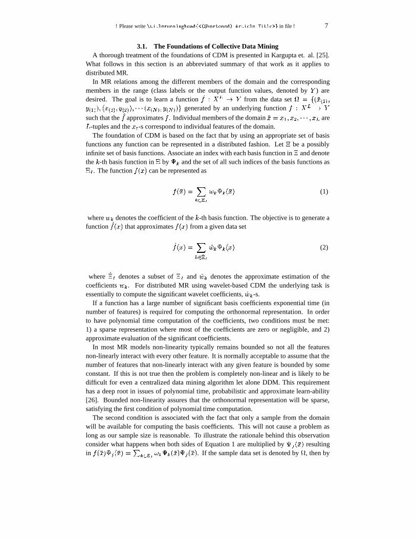
The Wavelet-Packet transform of a function in � + is calculated by recursively applyingthe quadrature filters to the and � coefficients of the next lower scale space and waveletspace as if each represented a separate scale space. Figure 3 shows how the wavelet-packettransform is generated by recursively applying the quadrature filters to the scale and waveletsubspaces. The vector � + �� + � � + �� + � ; input at the top level of the wavelet-packetdecomposition is formed by assuming that the observed values of the piece-wise constantfunction represent the coefficients of the scaling functions in � + . If the original functionis in � + then � + orthogonal subspaces �

�� 4 � � �� + ( 2 , will result from � recursiveapplications of � and � .

Using the Haar function wavelets partitions � + into � + orthogonal subspaces �� that

are each spanned by one of the first � + Walsh functions [17]. Therefore, the Walshfunctions form an orthogonal basis, � � �� ; , for � + and the Walsh coefficients,

. �� 4 � �� + ( 2 are equivalent to the wavelet-packet coefficients of the � + orthogonal

subspaces �� .3.3. The Wavelet-based CDM Approach to Local Regression

To demonstrate the wavelet-based CDM regression method consider again the naiveexample given in Section 2.3. Table 1 shows the Walsh coefficients, . � obtained from thewavelet-packet decomposition of � , � � , and � �� . Again selecting regression models

!� � � � � !� �� , !� � �� !� � �� and applying standard MR techniques to the non-zero Walshcoefficient sets in each partition gives,

!� � .�� . � � � � � � � � � � � �

10 ! Please write�� ! �"�#�$

in file !

� � � ��

� ��

� ��

� � ��

��

��

��

��

��

�

� �!�!� �#"%$'&

�)(+*

�)(-,

.

/�021304/ 57698;:=<�:=<�>@?�A*

,

B

, �

��

�� C

CC

CCC

CDC C CECFC"��G�!� "H�I$J&

FIG. 3. Application of quadrature filters in wavelet-packet decomposition.

and

!� � � .�� . � � � � � ( � � � � � ( � �

Note that 1) the representation of the information embodied in the example has be-come sparse compared to the original, 2) the regression coefficients for this decomposableproblem may now be determined directly from the non-zero wavelet coefficients in eachpartition without recourse to information exchange.

In the general case some information in the form of wavelet coefficients will need to becommunicated among partitions in order to resolve non-linear terms.

TABLE 1

Walsh (wavelet-packet) coefficients for naive example.

K L MONQPR L M�S � PR L M�S � PRT TFU T TFU T TFU TV TFU T TFU W TFU WX YFU T TFU Z TFU TY [�YFU T TFU T [�TFU Z

4. MULTIVARIATE LINER REGRESSION

Parametric regression [30], is a form of supervised learning that is applicable to CDM.In this section one approach to distributed MR based on an orthogonal wavelet basis ispresented. We begin with a description of the method used to generate local models,followed by the method for generating the global model. Next we apply these methods totwo benchmark data sets and compare the resulting model statistics with those obtainedusing standard MR techniques on centralized data sets. Following this, large synthetic datasets are employed to characterize model performance and scalability. Finally, we addressthe overall performance bounds for the methodology.


in file ! 11

4.1. Generating Local ModelsOne of the keys to CDM is that the local models represent local information in terms of

the coefficients of a function set that forms an orthogonal basis for the distributed data set.In the case of distributed MR the coefficients of interest are the Walsh (wavelet-packet)coefficients obtained by performing a wavelet-packet decomposition on the samples of eachfeature.

Given a partitioned set of real-valued features � � � �� and a data set of thesefeatures with * samples � � � � � �� &� �� let � � be the set of features and � bethe associated data set found in partition

�. If � �� then let � � � denote the column

vector of dimension * formed from the sample values of feature � in partition�

and� �� be the �� element of � � � .

Each of the � � � � � � may be transformed into a set of wavelet basis coefficients .� ��

using wavelet-packet decomposition. In terms of the wavelet-packet transform technique,

� � �� + � � � � �$2 � � + �� * � � + �therefore � � � � � + where in this case * � � + . Once the wavelet-packet transform of � � � is performed � � �� may be expressed in terms of the Walsh basis as

� � �� #� � .

� � � � �� (4)

If the wavelet functions are properly selected based on the feature sample characteristicsthe representation of the feature in the wavelet basis will be sparse and many of the . � -s willbe zero or insignificant. Note that the feature samples, � � �� , may be exactly re-constitutedfrom the wavelet coefficients using Equation 4. The wavelet representation may be mademore sparse by zeroing coefficients that have an absolute value below some threshold oralternatively retaining only a fixed number or percentage of the coefficients with the largestabsolute values. If the Walsh coefficients are ordered from largest to smallest absolutevalue and then the first �� * coefficients are retained Equation 4 becomes,

!� � �� #+ � .

� �� + -+��

where the index � is on the ordered coefficients. This thresholding process will eliminatethe ability to exactly re-constitute the feature sample values from the wavelet coefficients.However, a feature sample set estimate re-constituted from a set of thresholded coefficientswill be the minimum square error (MSE) estimate of the original feature samples based onthe number of wavelet coefficients retained [3]. The wavelet coefficients that remain afterthresholding form the local model.

4.2. Generating a Global Multivariate Regression ModelThe local model coefficients contain all of the information needed from the sample data

sets in order to generate a global model. These local model coefficients, representing a MSEestimate of the information available in the original feature samples, are communicated toa central site to facilitate the global model generation process. In order to generate theglobal model the wavelet coefficients for cross-terms and higher-order terms, the � � terms

12 ! Please write�� ! �"�#�$

in file !

in the function to be fit, must first be estimated. This may be accomplished directly fromthe local model wavelet coefficients.

To see that the wavelet coefficients for the cross-terms and higher-order terms may becalculated directly from the local model wavelet coefficients first recall that the waveletbasis functions are an orthogonal function set so that

2*� ; #� � � � �� -+ ��

� 2 if� � �

� otherwise(5)

where the �� are particular basis functions and N is the sample column vector spacesize. Certain sets of orthogonal basis functions such as Walsh are closed under productsuch that

� �� -+ �� (6)

For the case of the Walsh basis any set of Walsh functions satisfying equation 6 are relatedby

4 � �� (7)

where�

represents addition modulo 2 of the binary representations of the index values�

and � . Therefore in Equation 6 4 � � only if� � � , so it follows that

2*� ; #� � � � ��

� 2 if� � �

� otherwise

For feature � � the coefficient .� � � � for the 4 �� Walsh basis function is given by

.� � � � � 2

*� ; #� � � � � ��

and given a complete set of basis coefficients an individual sample value of feature � � maybe calculated using

� � �� ; #� � � . � � � � � �� (8)

For the cross-term � �� the relation for calculating the coefficient of the 4 �� basisfunction is

.�� 2

*� ; #� � � ��

and by substituting the relation for � � and �� based on Equation 8

.�� 2

*� ; #� � �

� � ; # � � � . � � � � � �� ; #+ � � . � � � + -+��


in file ! 13

Rearranging terms gives

.�� 2

*� ; # � � �

� ; #+ � � . � � � � .

� � � +� ; #� � � � �� + ��

Now note that the last sum in this relation will be zero unless � + � � or, equivalently,�� 4 . The sum may be replaced by the Dirac�-function

� ��

� � � � �� 2 if � � �

� otherwise

The relation for the cross-term basis function coefficient becomes

.�� 2

*� ; # � � �

� ; #+ � � . � � � � .

� � � + � �$� � � � � ( 4 �where again .

� � � � and .� � � + are wavelet-basis coefficients for features � � and � � , � �$� � �� ( 4 � is the Dirac delta function and * is the vector space dimension (the number of

samples). The relation for the cross-term basis coefficient is now in terms of only the basiscoefficients of the cross-term features.

Once the global model wavelet coefficients are available the regression coefficientsmay be estimated by performing a regression directly on the wavelet coefficients. This ispossible since the wavelet-packet transform is a linear transform. Thus the original functionestimation relation given in Section 2.3

!� � !� �� !� �� !�� is transformed linearly to

!.�� + � !� .

�� + � !� � .�� + � �� !� � .

�� +where .

�� + is the coefficient of the � �� basis function in the orthogonal representation of

the term � � of the function to be fit and the !� � coefficients we wish to estimate are thesame in both relations. Standard centralized MR techniques [30, 13] are used on the set of

wavelet coefficients .�� + to find the set of !� � -s that minimize % � .

�� + ( !.� *� + � �

.In Section 2 we noted that in terms of matrix notation, the estimates of the regression

coefficients could be calculated from the sample data as9-:� � , 7 , ��; < , 7��

In [4] the authors provide a detailed description of numerical methods for manipulatingmatrices to solve this specific equation. For the purposes of the work presented herehowever a somewhat similar approach, that is also presented in [4] was employed. Gaussianelimination was used to solve the 4 simultaneous equations

� � !� � � � !� � � �� !� � � � �� !� � � �� !� � � �� !� � � � � �

......

......

...� � !� � � � � !� � � �� !� � � � � �

14 ! Please write�� ! �"�#�$

in file !

where

� � + � #.� � . � � ( % .

� � % .� �

*

� � � � #.� � . �� ( % .

� � % .��

*It should be noted that while multivariate polynomial regression has been the model for

the mathematical development presented here, in general the terms � � of the function tobe fit may be non-polynomial functions of the feature set. In these situations additionaloperations in the form of these functions must be applied to the observed feature samplesor their wavelet coefficients. The most efficient order of application of the functions andwavelet transforms will depend on the form of the terms and the partitioning of the featureset.

As will be seen in the following section the accuracy of the global model decreasesas the number of cross-terms and higher-order terms increases for a given number offeatures and level of information communicated. This performance issue may be offset bya modification to the method used to generate the local models. In partition

�the terms� � �� 4 � � � of the polynomial dependent only on features in partition�

may beformed for each sample and the wavelet-packet decomposition calculated for each of these.This reduces the number of cross-terms and higher-order terms that must be estimatedusing local coefficients in the global model. The increase in global model accuracy is offsetby the increased communication cost associated with transmitting the local models of theterms in addition to those of the features. It must be emphasized that the accuracy of themethod is not directly dependent on the number of partitions but rather on the number ofcross-terms.

To summarize the wavelet-based CDM-MR method presented here

1. Calculate the wavelet basis coefficients for the features or terms in each partition,2. Use thresholding to select a subset of the largest absolute value coefficients for each

feature, creating a minimum square error model of the local features,3. Transmit the local coefficient models to a central site,4. Generate estimates of wavelet coefficients for cross-terms and/or higher order terms

directly from the local model coefficients, producing a global wavelet model,5. Calculate regression coefficients directly from the global wavelet coefficient model.

4.3. Application and Benchmarking of CDM RegressionIn this section we apply the CDM-MR technique to two benchmark data sets that have

been analyzed by others using standard MR techniques. The purpose is to demonstrate thespecifics of the CDM-MR technique on tractable data sets and to compare the parametricregression models obtained with published results for centralized data techniques.

We begin with data first proposed in [29] and currently included in the NIST StatisticalReference Datasets [31]. This data set consists of values of Total employment,GNP implicitprice deflater, GNP, Unemployment, Armed Forces manpower level, Non-institutionalizedpopulation � 14 yrs., and Year, for the years 1947 through 1962. The first of these sevenvariables (Employment) is taken as the dependent variable and the data set is used to fit aMR model with the six independent variables and an intercept. We deal with the intercept


in file ! 15

by adding a dummy feature to the problem. This feature has value 1 for all samples and theassociated regression coefficient in the wavelet basis will correspond to the intercept valuein the original basis.

The wavelet-packet decomposition for the “Year” independent variable is shown inFigure 4. The top ��

row is simply the sample data itself that is assumed to representthe coefficients �� through � � of the scaling functions. Since we are using Haar wavelets� � � � � � � � � � �� ; � � �$� the first entry in the � � � scale space is

��

�� 2��

�� 2��

��

�

Likewise, the first entry for the � � � wavelet space is

� �� ( � �

�� 2��

�( 2��

�� ( 2�

�

The second entry in each of the � � � spaces is

� � � ��

�and � � � � ��

�( � ��

�

with the other entries determined likewise. This process is repeated � � � 2 � �times, each

time starting with the scale and wavelet spaces is the previous step to produce the completewavelet-packet transform as shown in Figure 4. The complete set of � � � coefficients forthe dependent variable, the six independent variables, and the dummy feature variable areshown in Table 2.

The results obtained by performing a regression on the complete set of wavelet coeffi-cients is presented in Table 3. These results are, as expected, equivalent to the CertifiedRegression Statistics provided by NIST. Since all of the wavelet coefficients are used inthe regression a centralized regression is being performed. Statistics for MR models cre-ated using 12, 8 and 5 wavelet coefficients per feature are shown in Tables 4, 5 and 6,respectively. These results show the model parameters and statistics change as the numberof wavelet coefficients retained per feature approaches the minimum number required toproduce an , matrix of proper rank. It should be noted that the effect of eliminating asmall number of coefficients for this example is pronounced due to the small size of thedata set and the relatively high collinearity among the independent variables in the Long-ley data set. However, these models represent the minimum square error models for thenumber of wavelet coefficients per feature retained. The implications of this may be seenby comparing the CDM-MR model generated from the eight largest wavelet coefficientsfor each feature (Table 5) and a centralized model generated from some combination ofeight examples from the original data set. Tables 7 and 8 present the statistics for modelsgenerated with data samples for years 1947, 1949, 1953, 1954, 1955, 1956, 1960 and 1962,and for years 1947, 1948, 1949, 1950, 1959, 1960, 1961 and 1962. The statistics of thesethree models show some variation but the estimated regression coefficients for each modelfall within the 95% confidence interval for the other two models. Of particular interest is theinter-model variation in the size of the 95% confidence intervals. The second centralizedregression model has a much tighter confidence interval that the first centralized modeland the CDM-MR model has a tighter confidence interval that either of the centralizeddata models. This result demonstrates that selecting some subset of the sample data to

16 ! Please write�� ! �"�#�$

in file !

centralize and then use to generate a regression model may not generate the MSE modelfor that amount of information transfer. The result also supports the MSE model result forthe wavelet basis.

The second benchmark data set we employ is the Boston Housing data set created byHarrison and Rubinfeld [18]. This data set consists of 506 samples with 13 independentvariables, 12 of which are real-valued, and one real-valued dependent variable. Since theregression model reported in [18] has an intercept term we add one dummy variable with avalue of 1.0 for each sample to this data set. Descriptions of the variables are provided inTable 9. The regression model fit to the data is

� � � � � � � � � � � ��

� � �� (� � � � � ��

� � �� * � � � � *�� *��

The Longley data provided a good example of how overall model statistics comparebetween CDM-MR models and models created using centralized data. However, the dataset is to small to examine how the model changes as the number of wavelet coefficientsper feature retained to build the model is reduced. Using the Boston Housing data set wecompare the model produced with centralized data to models produced using 50%, 30% and10% of the coefficients per feature. Table 10 presents the results of the comparison. Thecentralized data results are taken from [18] except for the

� � value which was calculatedusing from the given coefficients and the data set. Overall, the CDM-MR model coefficientsremain consistent with the centralized model coefficients even at the 10% retained waveletcoefficients per feature level.

These data sets were selected to facilitate demonstration of the CDM-MR technique.They are not typical of the data sets that CDM is intended for in that they are small enoughto be stored at a single location and are complete in the sense that all features are under thedirect control of the investigator. The data sets CDM targets are very large with differentfeatures sets residing at different locations and possibly under the control of differententities. Inevitably, interesting data sets that fit this description are proprietary. In order toevaluated the performance of CDM-MR for larger data sets we turn in the following sectionto the use of synthetic data sets.

4.4. CDM Regression Method Performance TrendsIn this section we use several large (up to 100 MB) synthetic data sets to provide

a characterization of CDM-MR method performance trends in terms of 1) appropriateselection of wavelet functions, 2) the number of cross-terms and higher-order terms relativeto the number of features,3) the sample size for a given problem. In addition we demonstratescalability.

The basic metric we use to measure this performance is the residual value � defined by

� � ( !� � � �

where � � is the actual function or dependent feature value for example�

and !� � is theestimate of that value generated by the regression model. This is similar to the residualvalue calculated in classical parametric regression but has the important difference that theexamples used are from out-of-sample data not the examples used to build the regression


in file ! 17

�� !�� "�!�� !�� "�!�� FIG. 4. Wavelet-packet decomposition of Year variable from Longley data.

TABLE 2

Wavelet coefficients (j = 0) for Longley data.

Filter Y X1 X2 X3 X4 X5 X6 X7

HHHH 261268.0 4.0 406.725 1550793.75 12773.25 10426.75 469696.0 7818.0GHHH -12061.5 0.0 -35.475 -330374.25 -2176.75 -475.75 -22896.0 -16.0HGHH -5587.5 0.0 -19.625 -180627.75 -244.75 -1600.75 -11966.5 -8.0GGHH -816.0 0.0 -2.425 -3423.75 1362.25 -2038.25 2108.5 0.0HHGH -1068.0 0.0 -7.525 -64972.25 -1682.25 -71.75 -6475.5 -4.0GHGH 166.5 0.0 2.075 14241.75 -202.25 -140.25 1260.5 0.0HGGH 708.5 0.0 -2.275 5170.25 -439.25 196.75 1108.0 0.0GGGH 280.0 0.0 1.525 -3377.75 -28.25 -204.75 -355.0 0.0HHHG -829.0 4.0 -4.575 -36884.75 -540.25 -15.75 -2895.5 -2.0GHHG 326.5 0.0 -0.275 3168.25 -49.25 -83.25 645.5 0.0HGHG -169.5 0.0 -1.725 -700.25 -110.25 241.75 380.0 0.0GGHG -1143.0 0.0 -0.225 -17265.25 1061.75 -42.75 -310.0 0.0HHGG -1153.0 0.0 -1.625 -5499.75 621.25 -50.25 112.0 0.0GHGG 438.5 0.0 -0.925 -3944.75 166.25 -211.75 -81.0 0.0HGGG -485.5 0.0 -0.975 -3763.25 142.25 149.25 33.5 0.0GGGG 1417.0 0.0 -0.675 14615.75 -1229.75 280.75 67.5 0.0

model. The average residual value over the test data set

� 2�

�# � � �

� � ( !� � �

will remain close to zero unless the CDM-MR method introduces a bias or offset into themodel. The standard deviation of the residual values

# � � $%%& 2�( 2

�# � � �

� ( � �

provides a notion of the distribution of the residuals about the mean. As we are interestedonly in relative performance of the models the standard deviation of residual values fora set of models that are to be compared are normalized such that the maximum standarddeviation is 1.

Wavelets techniques form a large and expanding body of knowledge [19]. There are manyfamilies of wavelet functions. Any set of orthogonal wavelet functions may potentially beused in wavelet-based CDM. An important consideration in selecting a specific waveletfunction for a problem is how sparse the feature representation becomes in terms of thewavelet coefficients. As the representation becomes sparser fewer wavelet coefficientsare needed for a local model of a given accuracy. For this paper Haar wavelets wereselected because their relatively simple mathematical form provides a necessary clarity inthe development of the distributed MR technique. The Haar wavelets are the least-smoothmembers of the wavelet families they belong to.

18 ! Please write�� ! �"�#�$

in file !

TABLE 3

CDM Regression model statistics for Longley data with all coefficients retained.��

0.999987�� 304.8541

Coefficient�� P �� CI

��-3482258.7 890420.4 -3.9108 0.0036 -5496531.0, -1467986.3�� 15.0619 84.9149 0.1774 0.8631 -177.0292, 207.1529��

-0.0358 0.0335 -1.0695 0.3127 -0.1116, 0.0399�� -2.0202 0.4884 -4.1364 0.0025 -3.1251, -0.9154�� -1.0332 0.2143 -4.8220 0.0009 -1.5179, -0.5485�� -0.0511 0.2261 -0.2261 0.8262 -0.5625, 0.4603��

1829.1515 455.4785 4.0159 0.0030 798.7867, 2859.5162

TABLE 4

CDM Regression model statistics for Longley data with 12 coefficients retained.� �

0.999985�� 332.3977


��-3459035.5 896750.4 -3.8573 0.0039 -5487627.4, -1430443.5�� 56.1487 89.4239 0.6279 0.5457 -146.1424, 258.4398��

-0.0449 0.0316 -1.4186 0.1897 -0.1164, 0.0267�� -2.1178 0.4699 -4.5073 0.0015 -3.1808, -1.0549�� -1.0881 0.2429 -4.4794 0.0015 -1.6376, -0.5386�� 0.0373 0.2254 0.1653 0.8723 -0.4726, 0.5472��

1811.8521 460.4716 3.9348 0.0034 770.1922, 2853.5119

TABLE 5


0.999968�� 477.9735


��-2806889.6 1081972.7 -2.5942 0.0290 -5254483.9, -359295.4�� -24.3543 213.7620 -0.1139 0.9118 -507.9179, 459.2093��

-0.0216 0.0482 -0.4472 0.6653 -0.1306, 0.0875�� -1.7310 0.7048 -2.4561 0.0364 -3.3253, -0.1367�� -0.8998 0.4533 -1.9849 0.0784 -1.9253, 0.1257�� 0.0081 0.3599 0.0225 0.9826 -0.8060, 0.8222��

1478.6216 556.3516 2.6577 0.0261 220.0666, 2737.1767


in file ! 19

TABLE 6


0.999941�� 650.4082


��-3958376.7 3597783.7 -1.1002 0.2998 12097135.1, 4180381.6�� -1975.3736 1285.5059 -1.5367 0.1588 -4883.3922, 932.6450��

0.1719 0.1223 1.4055 0.1934 -0.1048, 0.4487�� -1.2519 0.6300 -1.9871 0.0782 -2.6771, 0.1733�� -0.4363 0.5620 -0.7765 0.4574 -1.7076, 0.8349�� -0.2650 1.3296 -0.1993 0.8464 -3.2729, 2.7428��

2145.8926 1896.6631 1.1314 0.2871 -2144.6608, 6436.4460

TABLE 7Standard regression model statistics for Longley data with 1947, 1948, 1949,

1950, 1959, 1960, 1961 and 1962 retained.� �

0.999665�� 191.1414


��-3401168.5 667110.9 -5.0984 0.1233 -11877579.8, 5075242.8�� -304.4729 211.3409 -1.4407 0.3863 -989.8016, 2380.8557��

0.0473 0.0455 1.0410 0.4872 -0.5305, 0.6252�� -0.9499 0.7564 -1.2558 0.4281 -10.5609, 8.6612�� -0.7709 0.4938 -1.5611 0.3627 -7.0456, 5.5038�� -0.8696 0.3721 -2.3370 0.2574 -5.5974, 3.8582��

1834.9335 342.7404 5.3537 0.1176 -2519.9775, 6189.8445

TABLE 8Standard regression model statistics for Longley data with 1947, 1949, 1953,

1954, 1955, 1956, 1960 and 1962 retained.��

0.998917�� 414.2000


�� -4951145.8 5312775.9 -0.9319 0.5224 -72456074.4, 62553782.9�� 276.7046 266.4325 1.0386 0.4880 -3108.6267, 3662.0359��

-0.1459 0.1829 -0.7978 0.5713 -2.4704, 2.1785�� -3.1734 2.6451 -1.1997 0.4424 -36.7822, 30.4355�� 0.7333 2.5085 0.2923 0.8190 -31.1405, 32.6070�� 0.6293 0.8046 0.7822 0.5774 -9.5938, 10.8525��

2548.0656 2719.4141 0.9401 0.5196 31890.8638, 36986.9950

20 ! Please write�� ! �"�#�$

in file !

TABLE 9

Variable definitions for Boston housing data set.

Variable Description

MV Median value of owner occupied homes.RM Average number of rooms per dwelling.AGE Proportion of owner-occupied units built prior to 1940.B Proportion of population that is black.LSTAT % of lower status of the population.CRIM Per capita crime rate.ZN Proportion of residential lad zoned for lots over 25,000 sq.ft.INDUS Proportion of non-retail business acres per town.TAX Full-value property-tax rate per $10,000.PTRATIO Pupil-teacher ratio by town.DIS Weighted distance to five Boston employment centers.RAD Index of accessibility to radial highways.NOX Nitric oxides concentration.

TABLE 10

Regression model results for Boston housing data set.

Parameter Centralized Model CDM Model - 50% CDM Model - 30% CDM Model - 10%� �

0.80569 0.804251 0.792491 0.775627�� 9.76 9.73 9.72 9.67�� 0.0063 0.0074 0.0090 0.0112�� 0.0000898 0.0004 -0.00079 -0.00067�� -0.19 -0.20 -0.23 -0.19�� 0.096 0.097 0.082 0.075�� -0.00042 -0.00042 -0.00033 -0.00039�� -0.031 -0.030 -0.027 -0.025�� 0.36 0.37 0.36 0.36�� -0.37 -0.36 -0.34 -0.28�� -0.012 -0.013 -0.013 -0.014�� 0.0000803 0.00032 0.00064 0.0016�� 0.000241 0.00031 0.00102 0.0016�� 0.088 0.084 0.119 0.118�� -0.0064 -0.0066 -0.0057 -0.0052


in file ! 21

0

0.1

0.2

0.3

0.4

0.5

0.6

0.7

0.8

0.9

1

10 20 30 40 50 60 70 80 90 100

Nor

mal

ized

Sta

ndar

d D

evia

tion

of R

esid

uals

Wavelet Coefficients Retained (%)

10% smooth20% smooth40% smooth60% smooth80% smooth

100% smooth

-0.4

-0.2

0

0.2

0.4

0.6

0.8

10 20 30 40 50 60 70 80 90 100

Mea

n R

esid

ual V

alue

(A

bsol

ute)

Wavelet Coefficients Retained (%)

10% smooth20% smooth40% smooth60% smooth80% smooth

100% smooth

FIG. 5. Model accuracy loss due to retention of fewer wavelet coefficients is reduced as the feature samplecharacteristics become more consistent with the smoothness of the wavelet function.

To demonstrate the importance of matching the wavelet function to the data characteris-tics we turn the problem on its head and apply the Haar based distributed MR to a seriesof data sets which provide varying degrees of suitability for use with the Haar wavelets.A function with 15 linear terms and four cross-terms (19 total terms) based of a featureset of size 15 was used for this purpose. Feature samples were generated randomly withuniform probability on the interval

( 2 � � ��2 � � � . The “smoothness” of the data was variedby introducing a probability that the sample value of each feature would change formone sample to the next. The smoothest data was generated with a 2�� probability thatfeature sample values would change from one sample to the next (barring the chance thatthe random number generator returned the same value). The least smooth data had only a2�� probability of individual sample values changing from one sample to the next. Testcases were performed with smoothness between 2�� and 2�� to evaluate the impact onglobal model accuracy as a function of percentage of wavelet coefficients retained in thelocal models. Figure 5 shows that for a given percentage of retained wavelet coefficientsthe less-smooth data sets tend to be more accurate since they are more compatible with thewavelet functions. The plots also show that global model accuracy, as measured by normal-ized residual value standard deviation and mean residual value increases as the percentageof wavelet coefficients retained increases.

In Figure 6 the effect of varying numbers of cross-terms relative to a fixed number offeatures is shown. The base function used in this evaluation was the same one used toevaluate the effect of data smoothness with additional cross-terms added as required by thecase. The feature sample data was 2�� smooth and the local models used 2 �� waveletcoefficient retention. Figure 6 shows a linear relation between the number of cross-termsand normalized residual standard deviation. The mean residual value remains close to zero.

The importance of sample size in CDM was described in Section 3 of this paper. Theeffect of sample size was evaluated using a 36-term quadratic in 15 features [25]. Inthe function each feature is represented in a linear and a quadratic term and there are sixadditional cross-terms,

� ��

� �� 2 �� ( �� 2�� 2 ��

2 � � � � 2�2 � �� 2 � � � ( 2 � � �� 2 �� ( ��

22 ! Please write�� ! �"�#�$

in file !

0

0.2

0.4

0.6

0.8

1

0 2 4 6 8 10 12 14 16 18 20

Nor

mal

ized

Sta

ndar

d D

evia

tion

of R

esid

uals

Cross-Terms Present

-0.4

-0.3

-0.2

-0.1

0

0.1

0.2

0.3

0.4

0.5

0.6

0 2 4 6 8 10 12 14 16 18 20

Mea

n R

esid

ual V

alue

(A

bsol

ute)

Cross-Terms Present

FIG. 6. Residual value standard deviation increases linearly while the mean residual value remains nearzero as the number of cross-terms increase

0.3

0.4

0.5

0.6

0.7

0.8

0.9

1

0 1000 2000 3000 4000 5000 6000 7000 8000 9000

Nor

mal

ized

Sta

ndar

d D

evia

tion

of R

esid

uals

Sample size

-600

-500

-400

-300

-200

-100

0

0 1000 2000 3000 4000 5000 6000 7000 8000 9000

Mea

n R

esid

ual V

alue

(A

bsol

ute)

Sample size

FIG. 7. Global model accuracy increases with sample size

�� 2 2 � �� 2�� ( �� ( 2 �� (

�� 2 � � �� ( 2 2 � � � �� ( 2�� ( 2 �� (

2 � � � ( 2 �� ( 2 � � � ( 2 �� ( 2��

�� (

�� 2 � � � � � ( ��

(��

��

Data sets were created with 2�� smoothness and between 1K and 8K training examplesand an equivalent number of test examples. Local models retained 2�� of the waveletcoefficients. Figure 7 shows that global model accuracy does increase as the sample sizeincreases.

To evaluate scalability of the CDM-MR algorithm a data set consisting of 193 features(1 dependent and 192 independent) and 64K samples was constructed. The dependentfeature was a function of 128 total terms, 64 linear terms and 64 cross-terms. The data setrepresents time-series data for three types of process. One third of the features are similarto the “ less smooth” data used in the other synthetic data sets. For this portion of the dataset the features take on values in

� ��2 � and change from sample to sample with probability

0.1%. The second third of the features evolve according to the process

� � � � � ( 2�# � � � � � � # � � )

where � ) is a Wiener process [20]. The sample data values are generated according to

� ��

; ��


in file ! 23

TABLE 11

Large data set calculations with various portions of coefficients retained.

% Coefficients Retained Mean residual Normalized standard deviation

100% 0.006 0.25250% -0.015 0.28130 % -0.007 0.40110% 0.023 1.000

where � is a random draw from a standard normal distribution and the specific values usedare � � � � � , # � � �� and � � � 2� � . The final third of the features evolve according tothe process � � � � � � ( � � � � � # � )where again � ) is a Wiener process [20]. The sample data values are generated accordingto

� �� ( � �

� � � � # � � � �where � is a random draw from a standard normal distribution, � � is set randomly on� � �� 2 � , � � � � and � � � �2 . For the second and third process

� � � �� .

The 64 linear terms in the regression function are based on the first third of the featuresand the 64 cross-terms are based on the products of the second and final third of thefeatures. The function value itself is the sum of the 128 terms plus a normally distributedrandom error. Calculations were performed with 100% , 50% , 30% and 10% of thewavelet coefficients for each feature retained. The results of the calculations are presentedin Table 11. The results show that for very large data sets the accuracy of the global model,as measured by the mean residual value and normalized standard deviation of residualsdoes not degrade significantly as the proportion of wavelet coefficients retained per featureis reduced to 10%.

It should be noted that it is currently rare to use parametric regression directly for afunction with this many terms. Principal components and/or factor analysis are typicallyused in this situation.

4.5. CDM Regression Algorithm PerformanceGiven * samples of each feature the wavelet-packet decomposition algorithm performs

* calculations for each of � � ��* decomposition levels resulting in a time complexity of� � * � � * � . If � features reside in a partition then it will take � � � * � � * � time tocalculated the coefficients for all the features in that partition.

Once all retained wavelet coefficients have been centralized it may be necessary tocalculate cross-term coefficients. Assuming that there are * samples, that � percent of thewavelet coefficients for each feature retained, and that the cross-terms depends on featuresin at most � partitions, then the worst-case performance will be � �$� ��* �� .

The regression algorithm as implemented for this work is dominated by the time neededto set up the simultaneous equations. Given

�independent regressors including the dummy

variable for the intercept term if needed the setup requires � � * � � � time.

5. LINEAR DISCRIMINANT ANALYSIS

24 ! Please write�� ! �"�#�$

in file !

Linear discriminant analysis (LDA) [13] is another form of supervised learning that isrelated to MR. Given two populations for which the same features are measured samplesfrom each population with known membership are used to construct a decision rule. Ob-servations with unknown population membership may be correctly classified with highprobability using the decision rule.

5.1. Linear Discriminant Analysis in CDMAn equivalence between MR and LDA was pointed out by Fisher [12]. Within the

regression model pseudo-variables representing the population classes are employed as thedependent variables. For a two-class problem:

� �� if observation

�comes from class 1

� � if observation�

comes from class 2

Fisher proposed that the values of the pseudo-variables be

� � � �� ; � � �

(�

� � � � (9)

where � and � � are the number of training examples from class 1 and 2, respectively.From a theoretical standpoint the difference between MR and Fisher’s LDA is that in

the case of MR the independent variables are assumed to be known exactly with anyvariability embodied in the dependent variable while in LDA the dependent variable (class)is known exactly and any variability is embodied in the independent variables. Froman implementation standpoint the important difference between MR and LDA is how themodel is used, not the basic CDM or regression techniques used to create the model. In thecase of LDA the result of applying the regression model to a set of features in an observationof unknown class is compared to a decision boundary value that is determined as part ofthe learning or training phase. By using the pseudo-variable values proposed by Fisherfor class values and with the assumption that the feature covariances are not significantlydifferent between populations the decision boundary value becomes 0.0. What constitutes asignificant difference in feature covariance between populations within the CDM frameworkand how this may be evaluated for any given populations is left for future resolution.

The following section describes an application of LDA to the Iris data set [12] a widelyused benchmark data set for statistics and machine learning.

5.2. CDM Linear Discriminant Analysis Example: Iris DataIn this section distributed LDA applied to the Iris data set [12] that consists of measure-

ments of four features of three varieties of Iris flower. The data set contains 150 examples,50 for each variety or class. Two samples were randomly eliminated from each classand the remaining 144 were divided into three groups of 48 samples each, 16 from eachclass, in order to facilitate a 3-fold cross validation of the model. For the purposes of thisdemonstration each feature is assumed to reside in a separate partition and the class labelcolumn vector is only needed to generate the global models so it is not transmitted to eachsite. Since the Iris data represents three classes, not two, an additional step is requiredin the modeling process. First regression models that discriminate between each pair ofclasses are generated then those models were used in committee form to select the properclassification for observations of unknown class. In the case of a tie (each model selects a


in file ! 25

different class) the estimated class value closest to the assigned class value for any modelis used to select the classification.

The results of the validation test cases are shown in Table 12. On average the modelscreated using wavelet-based CDM correctly classified the out-of-sample test cases � � ��of the time. Examples of reported accuracies for centralized methods are presented inTable 13.

TABLE 12

Results of 3-fold cross-validation on Iris data.

Case Correct Classification Incorrect Classification AccuracyV W�� T V T TFU T �X W V � �QW U T �Y W V � �QW U T �

CombinedV Y T V W � TFU Y �

It should be noted that because there are no cross-terms or higher-order terms onlyfour wavelet coefficients were required from each partition in order to generate the globalmodel. Thus the communication overhead was sightly over

� � of that required to centralizeall 96 sample values in any one training set at one site. Further, for this problem thecommunication cost of four wavelet coefficients is independent of the sample size. This isa result of the high level of compatibility between the discrete representation of the classvariable and the Haar wavelet functions.

6. CONCLUSIONS AND FUTURE WORK

This paper presents a method for performing distributed multivariate regression usingwavelet-based Collective Data Mining. The distributed multivariate parametric regressiontechnique presented here learns local information in terms of the coefficients of an orthog-onal basis function representation, transmits a small (relative to the sample size) numberof significant coefficients to a central site and then generates a global model directly fromthat small set of significant coefficients. The method seamlessly blends machine learningand the theory of communication with the statistical methods employed in multivariateparametric regression to provide an effective data mining technique for use in a distributeddata and computation environment.

In application to distributed multivariate parametric regression wavelet techniques wereshown to produce an orthogonal basis that provides a sparse, distributed, representation ofa function as basis function coefficients. Using these coefficients to communicate local

TABLE 13

Reported classification method accuracy for Iris data.

Method Accuracy Source

Clustering (ISODATA) 88.0% (Freemen, 1970) [14]Reduced-NN 93.0 - 96.7% (Gates, 1972) [15]1-NN 95 - 97% (Duda & Hart, 1973) [11]Partitional Clustering 89.337% (Duda & Hart, 1973) [11]Hierarchical Clustering 90.0% (Duda & Hart, 1973) [11]Tree 97.33% (Duda & Hart, 1973) [11]

26 ! Please write�� ! �"�#�$

in file !

model information to a central site required as little as 2 �� of the communication costrequired to assemble a centralized data set. The importance of selecting wavelet functionsthat are compatible with data characteristics, the reduction in model accuracy as the relativenumber of non-linear cross terms increases, and the increase in model accuracy with samplesize were demonstrated.

Application of wavelet-based CDM methodology to linear discriminant analysis, a tech-nique related to multivariate regression, was also presented. An application to the Iris dataset with the assumption that each feature resides in a different data base showed classifica-tion accuracy similar to centralized techniques. Linear discriminant problems such as Irisare particularly well suited for treatment with the Haar wavelets used in this work due to thediscrete nature of the class feature. Communication costs for this problem were shown tobe directly proportional to the number of independent features in the discriminant functionand independent of the sample size.

Future work will follow two distinct paths, further exploration of the use of wavelettechniques in this context and extension of these CDM techniques to other real-domainlearning problems.

The work presented in this paper is based on Haar wavelets and the Haar-Walsh waveletpacket basis. Higher order (smoother) orthogonal wavelets and other wavelet bases, suchas multi-resolution or Paley order, may provide improved performance in some cases.The ability to pre-characterize data sets in terms of appropriate wavelet function basis iscurrently being investigated.

Work on extending the real-domain wavelet-based CDM techniques to learning neuralnetwork models is ongoing.

ACKNOWLEDGMENTThe authors would like to acknowledge that this work is partially supported by a grant from the American

Cancer Society. The Boston housing data set used in Section 4 was obtained from the StatLib library maintainedby Carnegie Mellon University. The Iris data set used in the linear discriminant analysis presented in Section 5was obtained from the UCI repository of machine learning databases [2].

REFERENCES

1. J. M. Aronis, V. Kolluri, F. J. Provost, and B. G. Buchanan. The world: Knowledge discovery from multipledistributed data bases. Technical Report ISL-96-6, Intelligent Systems Laboratory, Department of ComputerScience, University of Pittsburgh, Pittsburgh, PA, 1996.

2. E. Blake, E. Keogh, and C.J. Merz. U.C.I. Repository of machine learning databases, 1998.

3. R. Carmona, Wen-Liang Hwang, and Bruno Torresani. Practical Time-Frequency Analysis, volume 9. Aca-demic Press, San Diego, 1998.

4. B. Carnahan, H. A. Luther, and J. O. Wilkes. Applied numerical methods. John Wiley and Sons, Inc., NewYork, 1969.

5. P. Chan and S. Stolfo. Experiments on multistrategy learning by meta-learning. In Proceeding of the SecondInternational Conference on Information Knowledge Management, pages 314–323, 1993.

6. P. Chan and S. Stolfo. Toward parallel and distributed learning by meta-learning. In Working Notes AAAIWork. Knowledge Discovery in Databases, pages 227–240. AAAI, 1993.

7. P. Chan and S. Stolfo. Toward scalable learning with non-uniform class and cost distribution: A case study incredit card fraud detection. In Proceeding of the Fourth International Conference on Knowledge Discoveryand Data Mining, page Not available. AAAI Press, September 1998.

8. J. Chattratichat, J. Darlington, Y. Guo, S. Hedvall, M. Kohler, A. Saleem, J Sutiwaraphun, and D. Yang.Toward scalable learning with non-uniform class and cost distribution: A case study in credit card frauddetection. In Proceeding of the Fourth International Conference on Knowledge Discovery and Data Mining,page Not available. AAAI Press, September 1998.


in file ! 27

9. D. Cheung, V. Ng, A. Fu, and Y. Fu. Efficient mining of association rules in distributed databases. IEEETransaction on Knowledge and Data Engineering, 8(6):911–922, 1996.

10. V. Cho and B Wuthrich. Toward real time discovery from distributed information sources. In Xingdong Wu,Ramamohanarao Kotagiri, and Kevin B. Korb, editors, Research and Development in Knowledge Discoveryand Data Mining, number 1394 in Lecture Notes in Computer Science : Lecture Notes in Artificial Intelligence,pages 376–377, New York, 1998. Springer-Verlag. Second Pacific-Asia Conference,PAKKD-98, Melbourne,Australia , April 1998.

11. R. O. Duda and D. E. Hart. Pattern classification and scene analysis. John Wiley and Sons, New York, 1973.

12. R. A. Fisher. The use of multiple measurements in taxonomic problems. Annals of Eugenics, 7:179–188,1936.

13. B. Flury and H. Riedwyl. Multivariate Statistics A Practical Approach. Chapman and Hall, New York, 1988.

14. J. J. Freemen. Experiments in discrimination and classification. Patterns Recognition, 1:207–218, 1970.

15. G. W. Gates. The reduced nearest neighbor rule. IEEE Transactions on Information Theory, 18(3):431–433,1972.

16. R. Grossman, S. Bailey, S. Kasif, D. Mon, A. Ramu, and B. Malhi. The preliminary design of papyrus: Asystem for high performance, distributed data mining over clusters, meta-clusters and super-clusters. FourthInternational Conference of Knowledge Discovery and Data Mining, New York, New York, Pages 37–43,1998.

17. H.F. Harmuth. Transmission of Information by Orthogonal Functions. Springer-Verlag, New York, 1972.

18. D. Harrison and D. L. Rubinfeld. Hedonic prices and the demand for clean air. Journal of EnvironmentalEconomics and Management, 5:81–102, 1978.

19. Barbara Burke Hubbard. The World According to Wavelets. A. K. Peters, Ltd., Wellesley, MA, 1998.

20. John C. Hull. Option, Futures, and Other Derivatives. Prentice Hall, Upper Saddle River, NJ, 1997.

21. H. Kargupta. Distributed knowledge discovery: A brief overview. In The Proceedings of the Spring 1999Symposium of the Institute for operations Research and the Management Sciences (INFORMS), May 1999.

22. H. Kargupta, I. Hamzaoglu, and B. Stafford. Scalable, distributed data mining using an agent based architec-ture. In David Heckerman, Heikki Mannila, Daryl Pregibon, and Ramasamy Uthurusamy, editors, Proceedingsof Knowledge Discovery And Data Mining, pages 211–214, Menlo Park, CA, 1997. AAAI Press.

23. H. Kargupta, I. Hamzaoglu, B. Stafford, V. Hanagandi, and K. Buescher. PADMA: Parallel data miningagent for scalable text classification. In Proceedings Conference on High Performance Computing ’97, pages290–295. The Society for Computer Simulation International, 1996.

24. H. Kargupta, E. Johnson, E. Riva Sanseverino, H. Park, L. D. Silvestre, and D. Hershberger. Scalable datamining from distributed, heterogeneous data, using collective learning and gene expression based genetic algo-rithms. Technical Report EECS-98-001, School of Electrical Engineering and Computer Science, WashingtonState University, 1998.

25. H. Kargupta, B. Park, D.E. Hershberger, and E. Johnson. Collective data mining: a new perspective towarddistributed data mining. Technical Report EECS-99-001, Washington State University, Department of Elec-trical Engineering and Computer Science, 1999. To be published in the book “Advances in Distibuted andParallel Knowledge Discovery.” Eds: Hillol Kargupta and Philip Chan.

26. S. Kushilevitz and Y. Mansour. Learning decision rees using fourier spectrum. In Proc. 23rd Annual ACMSymp. on Theory of Computing, pages 455–464, 1991.

27. W. Lam and A. M. Segre. Distributed data mining of probabilistic knowledge. In Proceedings of the17th International Conference on Distributed Computing Systems, pages 178–185, Washington, 1997. IEEEComputer Society Press.

28. W. Lee, S. Stolfo, and K. Mok. A data mining framework for adaptive intrusion detection. To appear in theProceedings of the 1999 IEEE Symposium on Security and Privacy, IEEE Computer Society Press, 1999.

29. J. W. Longley. An appraisal of least squares programs for the electronic computer from the viewpoint of theuser. Journal of the American Statistical Association, 62:819–841, 1967.

30. Frederick Mosteller and John W. Tukey. Data Analysis and Regression. Addison-Wesley, Menlo Park, CA,1977.

31. N.I.S.T. Statistical reference datasets.�� . Dataset Archives –

Linear Regression – Longley.

32. F.J. Provost and K. Venkateswarlu. A survey of methods for scaling up inductive learning algorithms. DataMining and Knowledge Discovery, 3(2):131–169, June 1999.

28 ! Please write�� ! �"�#�$

in file !

33. S. Stolfo et al. Jam: Java agents for meta-learning over distributed databases. In David Heckerman, HeikkiMannila, Daryl Pregibon, and Ramasamy Uthurusamy, editors, Proceedings Third International Conferenceon Knowledge Discovery and Data Mining, pages 74–81, Menlo Park, CA, 1997. AAAI Press.

34. Eric Stollnitz, Tony D. DeRose, and David H. Salesin. Wavelets for computer graphics: A primer, part 1.IEEE Computer Graphics and Applications, 5(3):76–84, May 1995.

35. Eric Stollnitz, Tony D. DeRose, and David H. Salesin. Wavelets for computer graphics: A primer, part 2.IEEE Computer Graphics and Applications, 5(4):75–85, June 1995.

36. R. Subramonian and S. Parthasarathy. An architecture for distributed data mining. Fourth InternationalConference of Knowledge Discovery and Data Mining, New York, New York, Pages 44–59, 1998.

37. M. V. Wickerhauser. Adapted Wavelet Analysis from Theory to Software. A. K. Peters Ltd., 1994.

38. D. Wolpert. Stacked generalization. Neural Networks, 5:241–259, 1992.

39. K. Yamanishi. Distributed cooperative bayesian learning strategies. In Proceedings of COLT 97, pages250–262, New York, 1997. ACM.

Documents

Distributed Multivariate Regression Using Wavelet-based Collective