Embed Size (px)
Citation preview
Multivariable Calculusand Real Analysis
(Student’s 2017/18 version)
These notes are not meant to cover exhaustively all of the material in the
course. They are meant to be used in addition to the lectures, to help
students to catch up if they missed some material and to read ahead of
the lectures if they so wish.
Dr. Anatoly Konechny
PUBLISHED BY PUBLISHER
BOOK-WEBSITE.COM
Licensed under the Creative Commons Attribution-NonCommercial 3.0 Unported License (the“License”). You may not use this file except in compliance with the License. You may ob-tain a copy of the License at http://creativecommons.org/licenses/by-nc/3.0. Unlessrequired by applicable law or agreed to in writing, software distributed under the License isdistributed on an “AS IS” BASIS, WITHOUT WARRANTIES OR CONDITIONS OFANY KIND, either express or implied. See the License for the specific language governingpermissions and limitations under the License.
First printing, January 2014
Contents
1 Limits . . . . . . . . . . . . . . . . . . . . . . . . . . . . . . . . . . . . . . . . . . . . . . . . . . . . . . . 7
1.1 Inequalities with modulus 71.1.1 Definition and general properties . . . . . . . . . . . . . . . . . . . . . . . . . . . . . . . . . . 71.1.2 Inequalities with moduli . . . . . . . . . . . . . . . . . . . . . . . . . . . . . . . . . . . . . . . . . . 81.1.3 Chains of inequalities . . . . . . . . . . . . . . . . . . . . . . . . . . . . . . . . . . . . . . . . . . . . 91.1.4 Moduli and square roots . . . . . . . . . . . . . . . . . . . . . . . . . . . . . . . . . . . . . . . . 10
1.2 Sequences 10
1.3 Limits of sequences 11
1.4 Limits of functions 16
2 Multivariable differential calculus . . . . . . . . . . . . . . . . . . . . . . . . . . . . 19
2.1 Functions of several variables 19
2.2 Limits and Continuity 222.2.1 Limits of functions of two variables . . . . . . . . . . . . . . . . . . . . . . . . . . . . . . . . 222.2.2 Continuity . . . . . . . . . . . . . . . . . . . . . . . . . . . . . . . . . . . . . . . . . . . . . . . . . . . 23
2.3 Differentiation 25
2.4 Graphs. Tangent Planes. 27
2.5 Higher order partial derivatives 33
2.6 The chain rule and partial derivatives. 36
2.7 Transforming equations. 38
3 Applications of partial derivatives . . . . . . . . . . . . . . . . . . . . . . . . . . . 41
3.1 Implicit functions. 41
3.2 Implicit differentiation. 423.2.1 More variables . . . . . . . . . . . . . . . . . . . . . . . . . . . . . . . . . . . . . . . . . . . . . . . . 43
3.3 Functions f : Rn→ Rm 46
3.4 Total derivatives 46
3.5 Various theorems about total derivatives 49
3.6 Taylor’s Expansion 51
3.7 Taylor’s formula in two dimensions 56
3.8 More applications 57
4 Double integrals . . . . . . . . . . . . . . . . . . . . . . . . . . . . . . . . . . . . . . . . . . . . 59
4.1 Double integrals 59
4.2 Interchanging the integration order 63
4.3 Calculating areas using double integrals 65
4.4 Change of variables in double integrals 66
4.5 Polar coordinates – continued 68
4.6 Other substitutions 70
5 Triple integrals . . . . . . . . . . . . . . . . . . . . . . . . . . . . . . . . . . . . . . . . . . . . . . 73
5.1 Triple integrals 73
5.2 Change of variables in triple integrals 775.2.1 Cylindrical polar coordinates (r,θ ,z) . . . . . . . . . . . . . . . . . . . . . . . . . . . . . . . 775.2.2 Spherical polar coordinates (r,θ ,φ) . . . . . . . . . . . . . . . . . . . . . . . . . . . . . . . . 80
5.3 Calculating volumes using triple integrals 82
5.4 Volumes of revolution 85
6 Integrals over unbounded regions and of unbounded functions 87
6.1 Integrals over infinite regions 87
6.2 Convergence of integrals 876.2.1 Integrals over unbounded intervals . . . . . . . . . . . . . . . . . . . . . . . . . . . . . . . . 876.2.2 Convergence tests for integrals over unbounded intervals . . . . . . . . . . . . . . 89
6.3 Convergence of integrals – continued 89
6.4 Integrals of unbounded functions 92
6.5 Convergence tests for integrals of unbounded functions 93
6.6 Multiple integrals over unbounded domains 94
6.7 Multiple integrals of unbounded functions 97
7 More applications of partial derivatives . . . . . . . . . . . . . . . . . . . . . . 99
7.1 Maxima and minima 997.1.1 Second derivative test for maxima and minima – one variable case . . . . . . 100
7.2 Second derivative test for two variables 101
7.3 Lagrange multipliers 104
7.4 More examples 107
Recommended books . . . . . . . . . . . . . . . . . . . . . . . . . . . . . . . . . . . . . 111
Books 111
Index . . . . . . . . . . . . . . . . . . . . . . . . . . . . . . . . . . . . . . . . . . . . . . . . . . . . . 113

Inequalities with modulusDefinition and general propertiesInequalities with moduliChains of inequalitiesModuli and square roots
SequencesLimits of sequencesLimits of functions
1 — Limits
1.1 Inequalities with modulus
There is no sharp distinction between calculus and analysis. Calculus is more focused on methodsof calculation while Analysis is occupied with rigorous definitions and qualitative questions ofthe type: "Is this function continuous?", "Does this sequence have a limit?" Answering suchqualitative questions most commonly involves solving inequalities. Often these inequalitiescontain absolute values or moduli of various quantities. In this section we review the basicproperties of the modulus and discuss how inequalities involving moduli can be solved.
1.1.1 Definition and general propertiesNotation 1.1. |x| denotes the modulus (aka absolute value) of x ∈ R, that is
|x|= x for x≥ 0 , |x|=−x for x < 0 .
For example, |3|= 3, |−2|= 2.
For any two numbers x,y ∈R, the distance between x and y is |x−y| (the modulus bit makessure that this is positive).
Corollary 1.1.1 — Facts about the modulus.
M1 −|x| ≤ x≤ |x| , |x|= |− x|M2 if a≥ 0, then: |x| ≤ a ⇔ −a≤ x≤ aM3 |x+ y| ≤ |x|+ |y| (triangle inequality)M4 |xy|= |x||y|.
Here are some examples of how these properties can be used
� Example 1.1 Show that |x−3| ≤ 0.2 ⇔ 2.8≤ x≤ 3.2.
Solution By M2,
|x−3| ≤ 0.2 ⇔ −0.2≤ x−3≤ 0.2 ⇔ 2.8≤ x≤ 3.2 .
�
8 Limits
� Example 1.2 Let a > 0. Show that if |x−a| ≤ a3 , then a
2 ≤ x≤ 3a2 .
Solution By M2,
−a2≤ x−a≤ a
2⇔ a
2≤ x≤ 3a
2.
�
� Example 1.3 Suppose that a,b,x,y,r ∈ R with r > 0, x 6= 0, b 6= 0. Show that if
|a− x| ≤ r2|b|
and |b− y| ≤ r2|x|
,
then
|ab− xy| ≤ r .
Solution
ab− xy = ab−bx+bx− xy = b(a− x)+ x(b− y)
⇒ |ab− xy|= |b(a− x)+ x(b− y)| ≤ |b(a− x)|+ |x(b− y)| (by M3)
= |b||a− x|+ |x||b− y| (by M4)
≤ r2+
r2= r .
�
1.1.2 Inequalities with moduliTo solve an inequality involving a variable means finding all possible values of that variablefor which the inequality is satisfied. Typically the allowed values correspond to collectionsof intervals. In the above examples 1.1 and 1.2 solutions to inequalities were worked out. Inexample 1.3 it was shown that two given inequalities imply a third one.
Sometimes inequalities contain more than one modulus. We will explain how to solve suchinequalities in the following example
� Example 1.4 Solve|2x−1|− |x+5|< 10 .
Inequalities involving one variable x and any number of absolute values can be solved in 3steps
1. Identify the values of x at which each absolute value vanishes. This breaks up the real lineinto a sequence of intervals.
2. Taking up one interval at a time we can get rid of the absolute values by replacing it eitherby the expression inside or the negative of that. We find solutions in each interval bysolving the "ordinary" inequalities.
3. We collect together all of the solutions we found in each interval.Let us apply this to the inequality above. The first modulus vanishes at x = 1/2 and the
second at x =−5. This gives us 3 intervals: (−∞,−5], [−5,1/2] and [1/2,∞). We take them upone after another.
1) On (−∞,−5] we have |2x−1|= 1−2x and |x+5|=−x−5. So that our inequality now reads
(1−2x)− (−x−5)< 10 .
1.1 Inequalities with modulus 9
We bring this tox >−4
This condition is inconsistent with the interval we are working on where x <−5. So there are nosolutions in this interval.
2) On [−5,1/2] interval we have |2x−1|= 1−2x and |x+5|= x+5 so that our inequality takesup the form
(1−2x)− (x+5)< 10 .
By standard manipulations we bring this to
x >−14/3 .
This gives us an interval of solutions x ∈ (−14/3,1/2] inside the interval we are working in.
3) On [1/2,∞) interval we have |2x−1|= 2x−1 and |x+5|= x+5 so that our inequality canbe written as
(2x−1)− (x+5)< 10
that we bring to the formx < 16
so that we obtain another interval of solutions x ∈ [1/2,16).
As a final step we collect all solutions we found and join in the adjacent intervals. We obtainthat all solutions are within a single interval x ∈ (−14/3,16). �
1.1.3 Chains of inequalitiesIf we are not interested in finding all solutions to a given inequality but rather in deriving(demonstraiting) that a certain inequality holds we proceed by working out a chain of inequalitiesof the type
something≤ something bigger≤ smth. bigger again≤ smth. simple .
Here are two concrete examples of these kind of chains
� Example 1.5 Show that∣∣∣2n+3
n2+6
∣∣∣≤ 5n for all n≥ 1.
Solution For n≥ 1,∣∣∣∣2n+3n2 +6
∣∣∣∣= 2n+3n2 +6
≤ 2n+3nn2 +6
≤ 5nn2 =
5n.
�
� Example 1.6 Show that∣∣ 1
2n−5
∣∣≤ 1n for all n≥ 5.
Solution For n≥ 5,∣∣∣∣ 12n−5
∣∣∣∣= 12n−5
(since 2n−5 > 0 for n≥ 5)
=1
n+(n−5)≤ 1
n(since n−5 > 0) .
�
10 Limits
Note that we can make a function bigger by throwing away something positive from thedenominator if the denominator is positive (thereby making the denominator smaller) as inExamples 1.5 and 1.6.
We cannot throw away something that is negative as this would make the denominator bigger.E.g. in Example 1.6, we cannot throw away the −5, i.e.
12n−5
1
2neven for 2n > 5 .
In fact,
12n−5
>12n
⇔ 2n > 2n−5 for 2n−5 > 0 .
1.1.4 Moduli and square rootsTaking a square root of a square of a number results in obtaining the modulus of that number
√a2 = |a| .
Often a wrong formula is used by students in which one puts just a on the right hand side. If a isnegative we may get a wrong answer. Here is an example of such a mistake.
� Example 1.7 Find all solutions to the equation
x2 = 4 .
Solution Since boths sides are non-negative we can take the square root of boths sides:√
x2 =√
4 = 2
If we set erroneously√
x2 = x then we obtain only one solution x = 2. While if we use thecorrect formula
|x|= 2
we obtain two solutions: x =−2, x = 2. �
1.2 SequencesDefinition 1.2.1 A sequence is an ordered list of real numbers.
� Example 1.8 Here are a few examples of sequences:1. 1, 1
2 ,13 ,
14 , . . .
2. 1,−1,1,−1, . . .3. 1
2 ,−14 ,
18 ,−
116 , . . .
4. 1,2,3,4, . . .5. 1,21/2,31/3, . . .6. 2,1,3,4,7,11,18, . . .
�
Note that the numbers in a sequence are arranged in a given order – if you change the order,you change the sequence. For any integer n ≥ 1, the number in position n in the sequence iscalled the n-th term of the sequence. If the n-th term in a sequence is denoted an, then thecomplete sequence is denoted by1 (an). Often, an is given by a formula involving n, but thereneed not exist a formula for general sequences.
1In some textbooks curly brackets are used: {an}.
1.3 Limits of sequences 11
Notation 1.2. N denotes the set of all positive integer numbers, i.e. N = {1,2,3, . . .}. Suchnumbers are called natural2. From now on, the letter n will denote a number in N.
� Example 1.9 — Example 1.8 continued. The sequences of Example 1.8 can be written:1.(1
n
)2.((−1)n+1
)3.((−1)n+1
2n
)4. (n)5.(n1/n
)6. ?
�
While the formula for the n-th term of the last sequence is not obvious the sequence isgenerated starting from the first two terms via the recurrence relation: an+1 = an +an−1. Thenumbers in the sequence are called Lucas numbers, they are a close relative of the Fibonaccinumbers.
Definition 1.2.2 A sequence (an) is called bounded if there exists K > 0 such that
|an| ≤ K for all n≥ 1 . (1.1)
Note that K must not depend on n. (an) is unbounded if it is not bounded.
� Example 1.10 — Example 1.8 continued.
1. bounded – K = 1 will do (or any number bigger than 1).2. bounded, K = 1.3. bounded, K = 1
2 .4. unbounded.5. unbounded – proof: for every K ≥ 0, there is an integer n > K, so |an|= n > K; hence the
definition is not satisfied, so the sequence is not bounded.6. bounded, but it is not easy to prove it.7. unbounded
�
1.3 Limits of sequencesConsider the question: does a sequence (an) approach a particular real number (the limit) as youmove further and further along it?
For example, take an = 1− 1n . Here, when n is “large”, an is “close” to 1. This is rather vague.
We need a precise definition which incorporates the following points:1. The sequence might never reach the limit (e.g. the above sequence (an) with an = 1− 1
napproaches 1 but never reaches it).
2. The sequence should “eventually” get as close as we choose to the limit.3. We do not care how far along the sequence we have to go in order to get “close” (as in 2.)
to the limit.Definition 1.3.1 A sequence (an) converges to a limit L ∈ R if, given any ε > 0 there existsa positive integer N = N(ε) such that |an−L|< ε for all n > N.
R Notes:2In some books zero is included into natural numbers.
12 Limits
1. an “close” to L here is taken to mean |an−L|< ε (i.e. L− ε < an < L+ ε) for eachε . Since ε can be chosen arbitrarily small an gets “arbitrarily close” to L.
2. “eventually” means for n > N, i.e. for n big enough.3. N generally depends on ε which is denoted by writing N = N(ε). If ε gets smaller,
N gets larger.
If no number L that fits the definition exists it is said that the limit does not exist or equiva-lently that the sequence at hand diverges.
Notation 1.3. If (an) converges to L, we write
limn→∞
an = L or an→ L as n→ ∞
(the n→ ∞ part indicates that n is getting larger and larger; the an→ L part indicates that an isapproaching L).
Often in analysis the following mathematical quantifiers (special symbols) are used:
Notation 1.4.
the symbol ∀ stands for "for all" or equivalently "for any"
Notation 1.5.the symbol ∃ stands for "there exists"
Also an implication is often denoted by an arrow: ⇒. Using these symbols the abovedefinition of a limit can be rewritten as follows:
limn→∞
an = L
means that ∀ε > 0 ∃N ∈ N such that ∀n > N |an−L|< ε .Let us look at some examples of how this definition can be used to rigorously prove that a
given sequence has a limit.
� Example 1.11 Prove that limn→∞
(1− 1
n
)= 1.
Solution We must use the definition. Here, an = 1− 1n , and the claim is that L = 1. Let ε > 0.
Then
|an−L|< ε ⇔ 1n< ε ⇔ n >
1ε.
Let N be an integer with N > 1ε. Then
n≥ N ⇒ n >1ε⇒ |an−L|< ε .
Thus, the definition is satisfied, and so we have proved that limn→∞
(1− 1
n
)= 1. �
� Example 1.12 Prove that limn→∞
2n−3n2+3n+1 = 0.
Solution Let ε > 0.∣∣∣∣ 2n−3n2 +3n+1
−0∣∣∣∣= ∣∣∣∣ 2n−3
n2 +3n+1
∣∣∣∣≤ 2n+3n2 +3n+1
≤ 2n+3nn2 =
5n,
hence |an−0|< ε if n > 5ε. Choosing N > 5
ε, we have
n≥ N ⇒∣∣∣∣ 2n−3n2 +3n+1
∣∣∣∣< ε ,
which proves the claim. �
1.3 Limits of sequences 13
R • We do not have to find the “best” N (whatever that means), so different choices of Ncan be equally valid. In particular, in a tutorial or exam situation, a different value ofN as compared to mine might be just as correct!
• To prove limn→∞
an = L, we typically follow a template:– First line: Let ε > 0.
– |an−L| ≤ · · · ≤ · · · ≤ something simple, typically a single negative power of n
– specify N
– Last line: n > N ⇒ |an−L|< ε .
Let us look at more examples
� Example 1.13 Prove that limn→∞
2n2+n+2n2+1 = 2.
Solution Let ε > 0.∣∣∣∣2n2 +n+2n2 +1
−2∣∣∣∣= ∣∣∣∣2n2 +n+2−2n2−2
n2 +1
∣∣∣∣= nn2 +1
<nn2 =
1n.
Let N ∈ N satisfy N > 1ε. Then if n≥ N,∣∣∣∣2n2 +n+2
n2 +1−2∣∣∣∣< 1
ε.
�
� Example 1.14 Prove that limn→∞
cosnn = 0.
Solution Let ε > 0. Since |cosn| ≤ 1, we have∣∣∣cosnn−0∣∣∣≤ 1
n< ε if n >
1ε.
Hence, choosing N > 1ε, we have
n≥ N ⇒∣∣∣cosn
n−0∣∣∣< ε .
�
Theorem 1.3.1 Any convergent sequence is bounded.
Proof Let (an) be a sequence with limn→∞
an = L. Let ε = 1 (actually, any other choice ofε > 0 would do, but let us choose ε = 1 for simplicity). Then by definition there exists anN ∈ N such that
n≥ N ⇒ |an−L|< 1 .
Thus, for n≥ N,
|an|= |an−L+L| ≤ |an−L|+ |L| (triangle inequality)
≤ 1+ |L| .
14 Limits
Now, let
M = max{|a1|, |a2|, . . . , |aN−1|} , K = max{M,1+ |L|} .
Then,
1≤ n≤ N−1 ⇒ |an| ≤M ≤ K
n≥ N ⇒ |an| ≤ 1+ |L| ≤ K ,
that is |an| ≤ K for all n (i.e. the definition of “bounded” is satisfied).
R The converse of Theorem 1.3.1 is not true.
� Example 1.15 ((−1)n) is bounded, but not convergent. �
To calculate limits of sequence the following theorem is instrumental
Theorem 1.3.2 If (an), (bn) are convergent sequences with limits A and B, respectively, then:(i) (an +bn) is convergent with limit A+B;
(ii) (anbn) is convergent with limit AB;(iii) (αan) is convergent with limit αA, for any α ∈ R;(iv) if bn 6= 0 for all n and B 6= 0, then
(anbn
)is convergent with limit A
B .Proof (i) follows straightforwardly from the triangle inequality for moduli. Let ε > 0.Since an→ A there exists a positive integer N = N(ε/2) such that |an−A| < ε/2 ∀n > N.Since bn→ B there exists a positive integer M = M(ε/2) such that |bn−B|< ε/2 ∀n > M.Therefore by triangle inequality
|an +bn−A−B|= |(an−A)+(bn−B)| ≤ |an−A|+ |bn−B|< ε
2+
ε
2= ε
for all integers n such that n > N and n > M. We can summarise both conditions by sayingthat n > K = max(N,M). Hence by definition an +bn→ A+B.
To prove (ii), let ε > 0.
|anbn−AB|= |an(bn−B)+B(an−A)| ≤ |an||bn−B|+ |B||an−A| .
Since the sequence (an) is convergent, it is bounded (by Theorem 1.3.1), so there exists K > 0such that |an|< K for all n. Thus,
|anbn−AB| ≤ K|bn−B|+ |B||an−A| .
We want to make the right hand side smaller than ε , so we would like to make both summandssmaller than ε
2 .By the definition of convergence:
there exists Na ∈ N such that n≥ Na ⇒ |an−A|< ε
2(|B|+1);
there exists Nb ∈ N such that n≥ Nb ⇒ |bn−B|< ε
2K.
1.3 Limits of sequences 15
Thus letting N = max{Na,Nb}, we have
n≥ N ⇒ |anbn−AB|< ε
2+
ε
2= ε .
The proofs of (iii) and (iv) are similar.
R In the previous examples, we were given L and had to prove convergence directly usingthe definition. By using Theorem 1.3.2, we can often find what L is and prove convergenceby looking at individual bits of a complicated expression and using known results, as inthe next example.
� Example 1.16
limn→∞
3n2−6n+25n2−2n+3
= limn→∞
3− 6n +
2n2
5− 2n +
3n2
=3−0+05−0+0
=53.
�
We finish this section with some additional examples.
� Example 1.17 Prove limn→∞
2n+5n3−5n2+n = 0.
Solution Let ε > 0. Consider
|an−L|=∣∣∣∣ 2n+5n3−5n2 +n
∣∣∣∣= 2n+5|n2(n−5)+n|
.
Since for n > 5 we have n2(n−5)> 0,
2n+5|n2(n−5)+n|
≤ 2n+5n2 · |n−5|
=2n+5
n2 ·∣∣n
2 +(n
2 −5)∣∣ .
Thus, for n≥ 10,
|an−L| ≤ 2n+5n3/2
≤ 2n+5nn3/2
=14n2 .
Since 14n2 < ε when n >
√14ε
, pick any integer N ≥ max{
10,√
14ε
}; then, for any n ≥ N,
|an−L|< ε . �
� Example 1.18 Prove
limn→∞
2n2 + e−n +(−1)n
(n+2)2−n · sin(n)= 2 .
Solution Let ε > 0. Consider
|an−L|=∣∣∣∣ 2n2 + e−n +(−1)n
(n+2)2−n · sin(n)−2∣∣∣∣= ∣∣∣∣e−n +(−1)n−8−8n+2n · sin(n)
n2 +4+n(4− sin(n))︸ ︷︷ ︸>0
∣∣∣∣≤∣∣∣∣e−n +(−1)n−8−8n+2n · sin(n)
n2
∣∣∣∣≤ e−n +1+8+8n+2n|sin(n)|
n2 (by triangle inequality)
≤ 1+1+8+8n+2nn2 =
10+10nn2 ≤ 10n+10n
n2 =20n.
16 Limits
Hence for N > 20ε
,
n≥ N ⇒ |an−L|< ε .
�
1.4 Limits of functionsLet f (x) be a function of one variable.
Definition 1.4.1 The limit of a function f at a point a is L, written
limx→a
f (x) = L
if for every ε > 0 there exists δ > 0 such that whenever 0< |x−a|< δ we have | f (x)−L|< ε .
Intuitively this definition means that we can take the value f (x) arbitrarily close to L by takingthe argument x sufficiently close (but not equal) to a.
R Notes:1. For functions that are not defined on the entire real line we should demand that x in
the above definition is from the domain of f . Note that a does not need to be fromthe domain. In some examples a lies on the boundary of the domain.
2. δ generally depends on ε which we can emphasize by writing δ = δ (ε). If ε getssmaller, δ gets smaller too.
3. When the limit L = limx→ a f (x) exists and the function f is defined at x = a, i.e.the value f (a) is specified, L may or may not coincide with f (a).
Here we give an example of how this definition can be used to show the existence (or absence)of limits for given f (x) and a:
� Example 1.19 Use ε , δ definition to show that
limx→1
(2−3x) =−1
Let ε > 0 be given. We need to have
| f (x)−L|= |(2−3x)− (−1)|= |3−3x|< ε
or equivalently−ε < 3−3x < ε
We rearrange this as−3− ε <−3x <−3− ε
Dividing all terms by −3 and reversing the inequalities we obtain
1− ε
3< x < 1+
ε
3
that means−ε
3< x−1 <
ε
3or equivalently |x−1|< ε
3.
To summarise we showed that the inequality |3−3x|< ε is satisfied (in this case it is equivalentto) whenever |x− 1| < ε
3 . Hence choosing δ = ε
3 we ensure that | f (x)− L| < ε whenever|x−a|< δ = ε
3 .�
1.4 Limits of functions 17
� Example 1.20 Show using the ε , δ definition that the limit
limx→0
x|x|
does not exist.Note that in this definition the function f (x) = x
|x| is defined only for x 6= 0 and the pointa = 0 we choose for examining the limit is not from the domain.
We start by observing that for any x > 0 f (x) = 1 and for any x < 0 f (x) =−1. Restrictingthe values of x to be within distance δ from a = 0 we thus have
f (x) = 1 if 0 < x < δ
f (x) =−1 if −δ < x < 0
The values 1 and −1 are two units apart, while for any possible limit L, the numbers L− ε
and L+ ε are 2ε apart and ε can be chosen arbitrarily. Therefore if ε < 1 (e.g. ε = 1/2) it isimpossible to have
L− ε < f (x)< L+ ε ∀x 6= 0 ,−δ < x < δ
for any choice of L and δ > 0. This contradicts the definition which requires that for any ε > 0(in particular including the values ε < 1) such δ > 0 should exist. Therefore the limit at handdoes not exist.
�
The notions of the limit of a sequence and the limit of a function at a point are related. Inparticular we can reformulate the notion of a limit of a function in terms of sequences. This isdone by the following theorem.
Theorem 1.4.1 Let f (x) be a function with domain D⊂ R (a subset of real numbers). Thefollowing two statements are equivalent
(i)limx→a
f (x) = L
(ii) For every sequence (xn) such that ∀n , xn ∈ D, xn 6= a and limn→∞
xn = a we have
limn→∞
f (xn) = L
Proof We first prove that (i) implies (ii). Suppose (i) holds. Then, given ε > 0 ∃δ = δ (ε)such that ∀x ∈ D
0 < |x−a|< δ ⇒ | f (x)−L|< ε . (1.2)
Suppose further that (xn) is a sequence such that ∀n , xn ∈ D ,xn 6= a and limn→∞
xn = a. This
means that taking δ chosen as above there exists a positive integer N = N(δ ) such that|xn− a| < δ ∀n > N. Since (1.2) is true for all x as long as |x− a| < δ we can apply it tox = xn that gives
| f (xn)−L|< ε ∀n > N .
Since ε was arbitrary this means that
limn→∞
f (xn) = L .
As this is true for all sequences xn satisfying the above conditions this proves (ii).
18 Limits
The proof of (ii)⇒ (i) is an example of a proof by contradiction which follows thefollowing pattern:• Suppose that the opposite of what you want to prove is true;• show that this supposition leads to a logical contradiction;• this implies that the supposition is false, so the statement you want to prove is true.Following the method assume that (ii) holds but that (i) is wrong. The latter means that
there exists ε > 0 such that for any δ > 0 there exists some x = x′ 6= a (which depends on δ )such that we simultaneously have
|x′−a|< δ and | f (x′)−L| ≥ ε .
Choose a sequence of positive numbers δn such that δn→ 0. By above for every δ = δn thereexists x′n 6= a such that
|x′n−a|< δn and | f (x′n)−L| ≥ ε .
Since this is true for any positive integer n we have
limn→∞
f (x′n) 6= L . (1.3)
On the other hand since δn → 0 for any ε ′ > 0 ∃N ∈ N such that δn < ε and therefore|x′n−a|< δn < ε . This means that
limn→∞
x′n = a (1.4)
Therefore (1.3) and (1.4) imply that (ii) is wrong. But since (ii) is assumed to hold oursupposition that (i) does not hold must be false. Therefore (ii) implies (i).
The last theorem shows that there are two equivalent definitions of the limit of a function:the ε , δ one and the one based on sequences. Although they are equivalent, using one rather thanthe other may be advantageous in solving particular problems.
The following theorem is very useful in calculating limits of functions
Theorem 1.4.2 Let f (x) and g(x) be two functions and let
limx→a
f (x) = L , limx→a
g(x) = M
then(i)
limx→a
( f (x)+g(x)) = L+M
(ii)limx→a
( f (x) ·g(x)) = LM
(iii)
limx→a
f (x)g(x)
=LM
if M 6= 0
Proof The proof of this theorem follows from a combination of results of Theorem 1.3.2and Theorem 1.4.1 that allows us to use sequences to define limits of functions.
Functions of several variablesLimits and Continuity
Limits of functions of two variablesContinuity
DifferentiationGraphs. Tangent Planes.Higher order partial derivativesThe chain rule and partial derivatives.Transforming equations.
2 — Multivariable differential calculus
2.1 Functions of several variables
A function f (x) of one variable is a rule taking a single number x and producing a new numberf (x), e.g. f (x) = x2 or f (x) = sin(x). Similarly, a function of two variables f (x,y) is a ruletaking two numbers x,y and producing a new number f (x,y), e.g.
f (x,y) = x2 + sin(y)
f (x,y) = x2y3 .
We do not have to stop at two variables, e.g. f (x,y,z) = x2y3z5 is a function of three variables.More generally,
f (x1,x2, . . . ,xn) = x1 + x2 + . . .+ xn (2.1)
is a function of n variables. Usually, for two and three variables, we will use the notation x,y orx,y,z, respectively, while for more variables we will use subscripts such as in xi.
We will often write
f : Rn→ R (2.2)
to say that f is a function of n variables taking values in the real numbers.
R Reminder:• R – the set of all real numbers• Z – the set of all integers• N – the set of all natural numbers (1,2,3, . . .)• Q – the set of all rational numbers
Sometimes a function does not make sense for arbitrary values of the variables and can onlybe defined on a restricted set called its domain.
R Reminder: Domains of some elementary functions:• f (x) = xµ
20 Multivariable differential calculus
1. For µ ≥ 0, and µ ∈ Z or µ = mn ∈Q (where m,n ∈ Z, and where Q denotes the
rational numbers) with n odd,
D f = R1 ,
e.g. f (x) = x2/3.2. for µ < 0, and µ ∈ Z or µ = m
n ∈Q with n odd,
D f = {x ∈ R1 | x 6= 0} ,
e.g. f (x) = x−3/5.3. for µ > 0, and when µ is irrational or for µ = m
n ∈Q with n even,
D f = {x | x ∈ R , x≥ 0} ,
e.g. f (x) = x1/2 or f (x) = x√
2.4. for µ < 0 when µ is irrational or µ = m
n ∈Q with n even,
D f = {x | x ∈ R , x > 0} ,
e.g. f (x) = x−π or f (x) = x−1/4.• f (x) = loga(x) is defined for x > 0.
We write
f : D f → R
or
f : D→ R
to say that f takes numbers from the domain D f ⊂ Rn and assigns to them numbers in R.
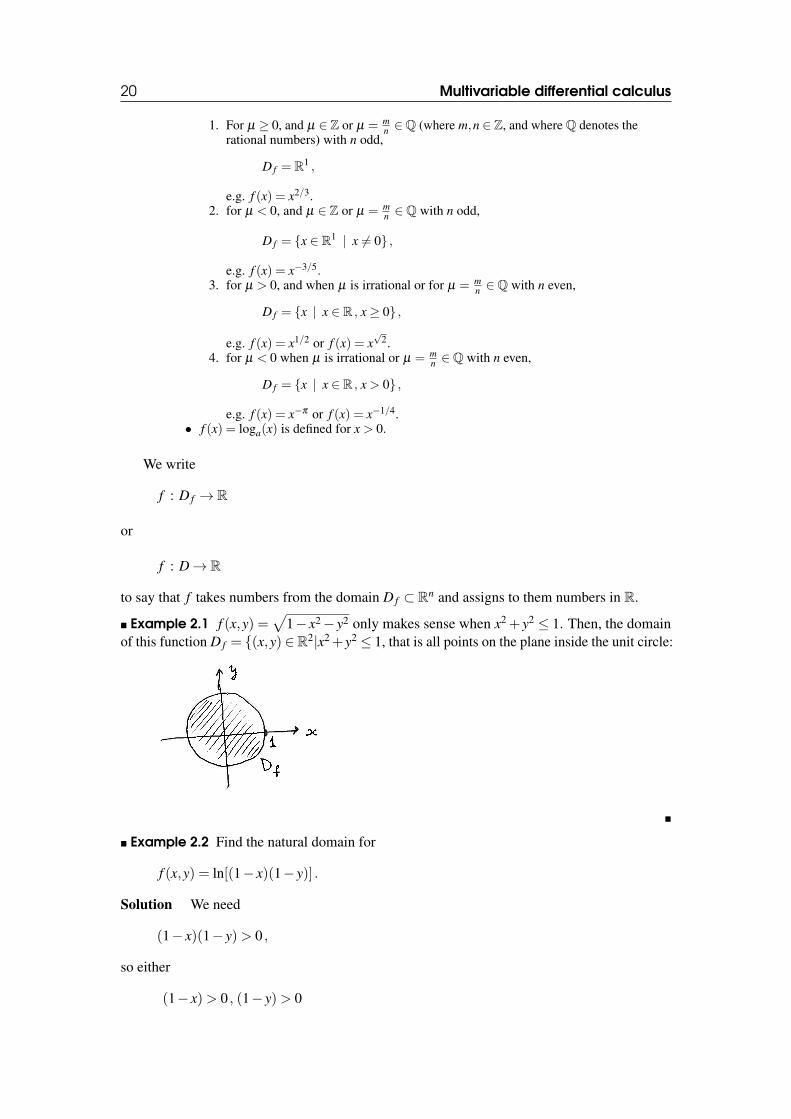
� Example 2.1 f (x,y) =√
1− x2− y2 only makes sense when x2 + y2 ≤ 1. Then, the domainof this function D f = {(x,y) ∈R2|x2+y2 ≤ 1, that is all points on the plane inside the unit circle:
�
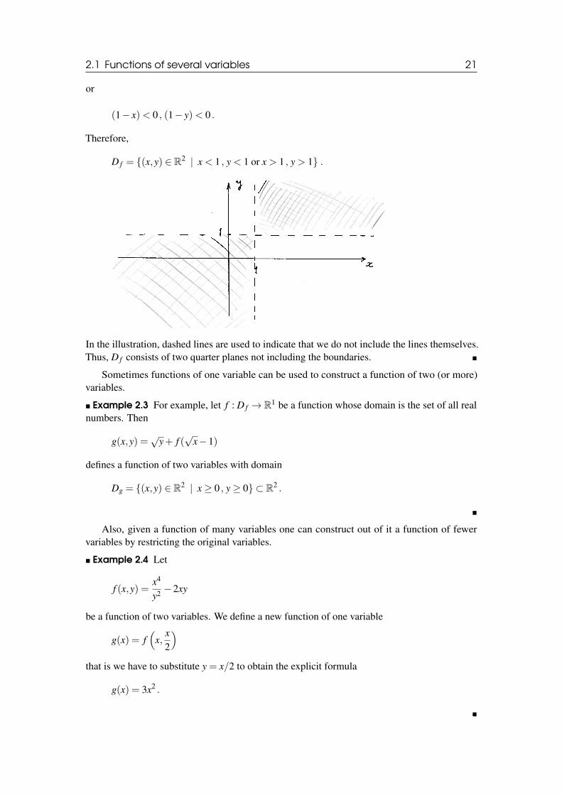
� Example 2.2 Find the natural domain for
f (x,y) = ln[(1− x)(1− y)] .
Solution We need
(1− x)(1− y)> 0 ,
so either
(1− x)> 0 , (1− y)> 0
2.1 Functions of several variables 21
or
(1− x)< 0 , (1− y)< 0 .
Therefore,
D f = {(x,y) ∈ R2 | x < 1 , y < 1 or x > 1 , y > 1} .
In the illustration, dashed lines are used to indicate that we do not include the lines themselves.Thus, D f consists of two quarter planes not including the boundaries. �
Sometimes functions of one variable can be used to construct a function of two (or more)variables.
� Example 2.3 For example, let f : D f → R1 be a function whose domain is the set of all realnumbers. Then
g(x,y) =√
y+ f (√
x−1)
defines a function of two variables with domain
Dg = {(x,y) ∈ R2 | x≥ 0 , y≥ 0} ⊂ R2 .
�
Also, given a function of many variables one can construct out of it a function of fewervariables by restricting the original variables.
� Example 2.4 Let
f (x,y) =x4
y2 −2xy
be a function of two variables. We define a new function of one variable
g(x) = f(
x,x2
)that is we have to substitute y = x/2 to obtain the explicit formula
g(x) = 3x2 .
�
22 Multivariable differential calculus
� Example 2.5 With the relation between f and g as in example 2.3, determine the explicitforms of f and g given that
g(x,1) = x .
Solution
g(x,1) = 1+ f (√
x−1) = x
⇒ f (√
x−1) = x−1
⇒ g(x,y) =√
y+ x−1 .
To determine f explicitly, let w =√
x−1. Then√
x = 1+w, and for x≥ 0
x = (1+w)2 .
Hence f (w) = (1+w)2−1 = w2 +2w. This is the explicit form of f . �
2.2 Limits and Continuity2.2.1 Limits of functions of two variables
The ε-δ definition 1.4.1 of a limit for a function of one variable extends to functions of twovariables in the following way.
Definition 2.2.1 Let f by a function of two variables with domain D f ⊂ R2. We say that fhas a limit at (a,b) ∈ R2 (not necessarily from the domain D f ) with the value L and write
lim(x,y)→(a,b)
f (x,y) = L
if for every ε > 0 there exists δ > 0 such that whenever (x,y) ∈ D f and
0 < |x−a|< δ , 0 < |y−b|< δ
we have | f (x)−L|< ε .
Similarly to Theorem 1.4.1 there is an equivalent definition of a limit of function of twovariables in terms of sequences:
Theorem 2.2.1 Let f (x) be a function of two variables with domain D f . The following twostatements are equivalent
(i)lim
(x,y)→(a,b)f (x) = L
(ii) For every pair of sequences (xn,yn) such that ∀n , (xn,yn) ∈ D f , (xn,yn) 6= (a,b) and
limn→∞
xn = a , limn→∞
yn = b
we havelimn→∞
f (xn,yn) = L
The proof of this theorem is similar to the proof of Theorem 1.4.1 and we will omit it.
� Example 2.6 Consider a function
g(x,y) =x2− y2
x2 + y2
2.2 Limits and Continuity 23
defined for (x,y) 6= (0,0). Show that the following limit does not exist
lim(x,y)→(0,0)
g(x,y) .
Solution To show that the limit does not exist it suffices to present two sequences of pointsfrom the domain which both tend to the origin but for which the limits of values (if exist) aredifferent. Choosing first (xn,yn) = (1/n,1/n)→ (0,0) we find
limn→∞
f (1n,1n) = lim
n→∞
1n2 − 1
n2
1n2 +
1n2
= limn→∞
0 = 0 .
Choosing next (xn,yn) = (1n ,0)→ (0,0) we obtain
limn→∞
f (1n,0) = lim
n→∞
1n2 −02
1n2 +02
= limn→∞
1 = 1 .
Since these are two different numbers the limit at hand does not exist. �
We end this subsection by remarking that definition 2.2.1 and theorem 2.2.1 generalise tothree and more variables in a straightforward manner.
2.2.2 ContinuityRecall the definition of continuity for functions of one variable:
Definition 2.2.2 — Continuity. A function f (x) is said to be continuous at a point x = a if
limx→a
f (x) = f (a) .
It is assumed in the above definition that a ∈ D f . The limit limn→∞
f (xn) must exist and must be
equal to the value f (a).
A function continuous at any point in its domain is called continuous.Similarly to the above, a function of two variables f (x,y) with domain D f ⊂ R2 is called
continuous at a point (a,b) ∈ D f if
lim(x,y)→(a,b)
f (x,y) = f (a,b) .
24 Multivariable differential calculus
In view of Theorem 2.2.1 this is equivalent to saying that for any sequences xn→ a and yn→ bsuch that (xn,yn) ∈ D f for all n, the limit lim
n→∞f (xn,yn) exists and
limn→∞
f (xn,yn) = f (a,b) .
The above definitions generalise to 3 and more variables in a straightforward manner. Usingvector notation with x ∈ Rn. Given a function f of n-variables it is said to be continuous at apoint a ∈ Rn from its domain if
limx→a
f (x) = f (a) .
� Example 2.7 Consider a function of two variables
f (x,y) :=
{xy
x2+y2 for (x,y) 6= (0,0)
0 for (x,y) = (0,0)
defined on the entire R2. Show that this function is not continuous at (x,y) = (0,0). SolutionLet xn =
1n , yn = 0 and n ≥ 1 such that (xn,yn) approaches the point (0,0) along the x-axis as
n→ ∞. Then
limn→∞
xnyn
x2n + y2
n= lim
n→∞0 = 0 .
Now let xn =1n as before and yn =
1n , again with n > 1. Then
limn→∞
xnyn
x2n + y2
n= lim
n→∞
1n ·
1n
1n2 +
1n2
=12.
Thus, depending on how we approach the point (0,0), we get different limits. In particularfor the last sequence the limit lim
n→∞f (xn,yn) =
12 6= f (0,0) = 0, and we conclude that f is not
continuous at the point (0,0). �
It is not hard to show that the above function is continuous at every point (x,y) ∈ R2 exceptfor (x,y) = (0,0), which is thus an isolated discontinuity. In general, discontinuities can beconcentrated on curves for functions of two variables, on surfaces for functions of three variablesand so on.
� Example 2.8 The function
h(x,y) :=
{x2+y2
x2−y2 for x2 6= y2
1 for x2 = y2
has a discontinuity along a pair of lines ±x = y. (This means that for each point on this pair oflines function h is not continuous at it.) The function of three variables
g(x,y,z) :=
{1
x2+y2+z2−1 for x2 + y2 + z2 6= 1
0 for x2 + y2 + z2 = 1
is discontinuous on a sphere defined via
x2 + y2 + z2 = 1 .
�
2.3 Differentiation 25
R Note that to prove that a function is not continuous at a given point it is convenient touse the sequential definition of a limit of a function while to show that the function iscontinuous one typically uses the ε-δ definition. In general there is no straightforward(mechanical) way to determine whether the given function is or is not continuous at a givenpoint and one needs to investigate the problem both ways (i.e. if you tried to show that thefunction is not continues using sequences but failed perhaps it is not. Then you changestrategry and try to show that it is continuous using the ε and δ definition).
R Polynomials in any number of variables are continuous at any point. Rational functionsare continuous at any point where they are defined, i.e. excluding the points where thedenominator vanishes but the numerator does not.
Sometimes we may have points which are not in the domain but at which the limit of thefunction exists. Such point can be added to the domain by assigning the value of the function tobe given by the value of the limit. This is called extension by continuity as we extend the domainby adding a new point in such a way that the function is continuous at that point.
� Example 2.9 Determine whether the function
f (x,y) = xy
defined for x > 0 and y > 0, can be made continuous at (0,0). (In other words determine whetherthe domain of f can be extended by continuity to include (0,0).)
Solution The value of the function at (0,0) is not defined. Can we modify the definition of fsuch that the function becomes continuous? Note that
f (0,y) = 0y = 0
for any y > 0, thus picking (xn,yn) = (0, 1n)→ (0,0) we get
limn→∞
f (xn,yn) = limn→∞
01n = lim
n→∞0 = 0 .
On the other hand, for (xn,yn) = (1n ,0)→ (0,0),
limn→∞
f (xn,yn) = limn→∞
(1n
)0
= limn→∞
1 = 1 .
We can choose to assign f (0,0) to be 0 or 1 (or any other number), but f cannot be madecontinuous. �
2.3 DifferentiationConsider f : R2→ R (a function of two variables) and let (x0,y0) ∈ R2. The partial derivativesof f at (x0,y0) denoted
∂ f∂x
(x0,y0) ,∂ f∂y
(x0,y0)
are defined as
∂ f∂x
(x0,y0) = lim∆x→0
f (x0 +∆x,y0)− f (x0,y0)
∆x,
∂ f∂y
(x0,y0) = lim∆y→0
f (x0,y0 +∆y)− f (x0,y0)
∆y.
(2.3)
26 Multivariable differential calculus
This means that to define ∂ f∂x we consider f (x,y) as a function of x only, keeping y = y0 fixed,
and differentiate with respect to x at the point x0 as a function of one variable. Similarly, todefine ∂ f
∂y one fixes x and differentiates with respect to y at y0.
� Example 2.10 For
f (x,y) = x2 + y3 ,
fix y = y0, and consider
f (x,y0) = x2 + y30
as a function of x only. Then in differentiating it with respect to x, we treat y30 as a constant,
hence∂ f∂x
(x0,y0) = 2x0 .
Similarly, fixing x = x0 we consider
f (x0,y) = x20 + y3
as a function of y only, and obtain
∂ f∂y
(x0,y0) = 3y20 .
�
Often we do not care about a specific point (x0,y0) and we just work out ∂ f∂x (x,y),
∂ f∂y (x,y) at
any point (x,y). In this case we often just write
∂ f∂x
,∂ f∂y
.
Other alternative notations are
fx, fy
and
fx(x,y) , fy(x,y) .
� Example 2.11 For
f (x,y) = x3 +3xy+ y2 ,
we calculate
fx =∂ f∂x
=∂ f∂x
(x,y) = 3x2 +3y ,
fy =∂ f∂y
=∂ f∂y
(x,y) = 3x+2y ,
For
f (x,y) =xy,
we calculate∂ f∂x
=1y,
∂ f∂y
=− xy2 .
Similarly, if f : Rn→ R we define ∂ f∂xi
for each label i = 1,2, . . . ,n. �
2.4 Graphs. Tangent Planes. 27
� Example 2.12 For
f (x1,x2,x3,x4) = x21 + x3
2 + x43 + x5
4
we have
∂ f∂x3
= 4x33 .
For
f (x,y,z) = xy ln(z)
we have
∂ f∂ z
=xyz.
�
� Example 2.13 For
f (x,y) = xy ,
find fx, fy.
Solution To find fx, we fix y. Then xy is just an ordinary power function of x so that
fx =∂xy
∂x= y · xy−1 .
To find fy, we first rewrite f as
f (x,y) = ey ln(x) .
Treating x as a constant and using chain rule we obtain
fy =∂ey ln(x)
∂y= ln(x) · ey ln(x) = ln(x) · xy .
�
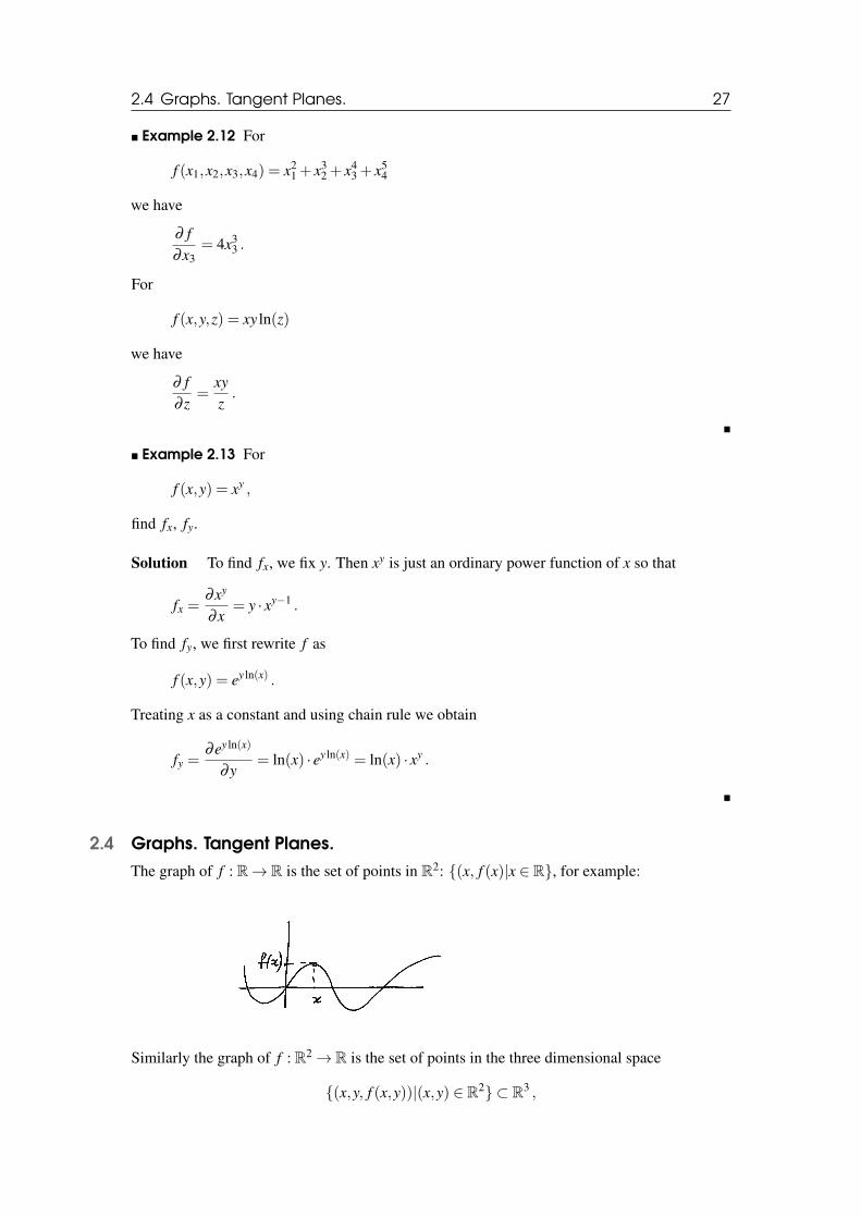
2.4 Graphs. Tangent Planes.The graph of f : R→ R is the set of points in R2: {(x, f (x)|x ∈ R}, for example:
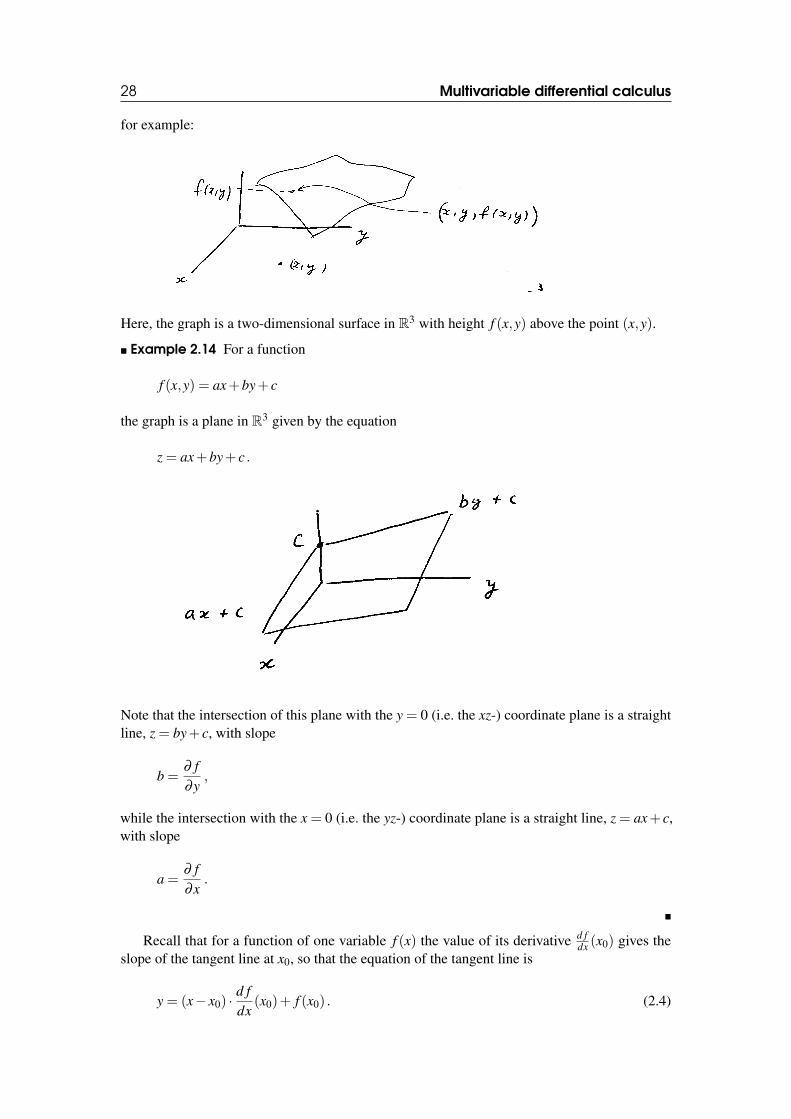
Similarly the graph of f : R2→ R is the set of points in the three dimensional space
{(x,y, f (x,y))|(x,y) ∈ R2} ⊂ R3 ,
28 Multivariable differential calculus
for example:
Here, the graph is a two-dimensional surface in R3 with height f (x,y) above the point (x,y).
� Example 2.14 For a function
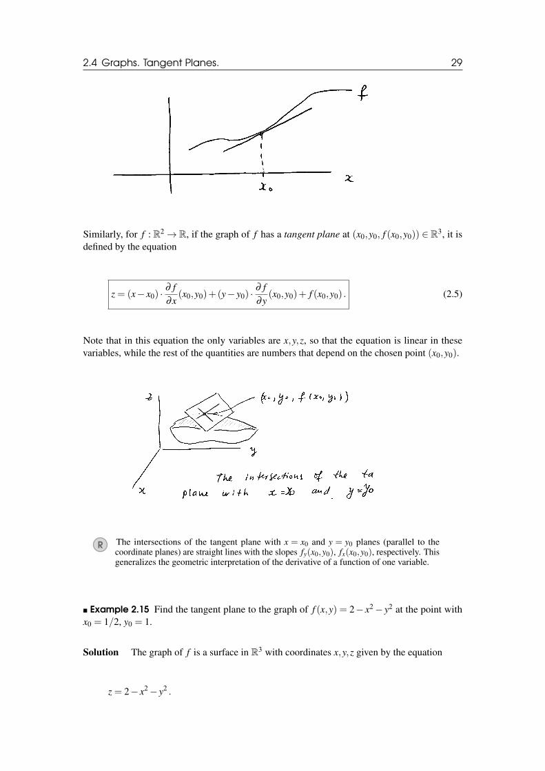
f (x,y) = ax+by+ c
the graph is a plane in R3 given by the equation
z = ax+by+ c .
Note that the intersection of this plane with the y = 0 (i.e. the xz-) coordinate plane is a straightline, z = by+ c, with slope
b =∂ f∂y
,
while the intersection with the x = 0 (i.e. the yz-) coordinate plane is a straight line, z = ax+ c,with slope
a =∂ f∂x
.
�
Recall that for a function of one variable f (x) the value of its derivative d fdx (x0) gives the
slope of the tangent line at x0, so that the equation of the tangent line is
y = (x− x0) ·d fdx
(x0)+ f (x0) . (2.4)
2.4 Graphs. Tangent Planes. 29
Similarly, for f : R2→ R, if the graph of f has a tangent plane at (x0,y0, f (x0,y0)) ∈ R3, it isdefined by the equation
z = (x− x0) ·∂ f∂x
(x0,y0)+(y− y0) ·∂ f∂y
(x0,y0)+ f (x0,y0) . (2.5)
Note that in this equation the only variables are x,y,z, so that the equation is linear in thesevariables, while the rest of the quantities are numbers that depend on the chosen point (x0,y0).
R The intersections of the tangent plane with x = x0 and y = y0 planes (parallel to thecoordinate planes) are straight lines with the slopes fy(x0,y0), fx(x0,y0), respectively. Thisgeneralizes the geometric interpretation of the derivative of a function of one variable.
� Example 2.15 Find the tangent plane to the graph of f (x,y) = 2− x2− y2 at the point withx0 = 1/2, y0 = 1.
Solution The graph of f is a surface in R3 with coordinates x,y,z given by the equation
z = 2− x2− y2 .
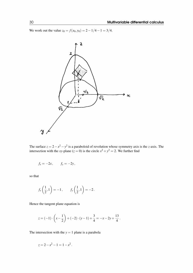
30 Multivariable differential calculus
We work out the value z0 = f (x0,y0) = 2−1/4−1 = 3/4.
The surface z = 2− x2− y2 is a paraboloid of revolution whose symmetry axis is the z-axis. Theintersection with the xy-plane (z = 0) is the circle x2 + y2 = 2. We further find
fx =−2x , fy =−2y ,
so that
fx
(12,1)=−1 , fy
(12,1)=−2 .
Hence the tangent plane equation is
z = (−1) ·(
x− 12
)+(−2) · (y−1)+
34=−x−2y+
134.
The intersection with the y = 1 plane is a parabola
z = 2− x2−1 = 1− x2 .
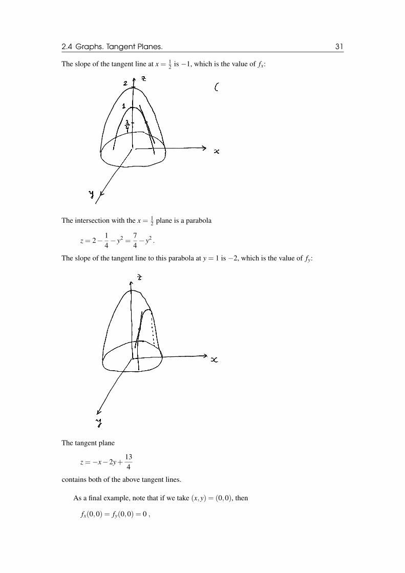
2.4 Graphs. Tangent Planes. 31
The slope of the tangent line at x = 12 is −1, which is the value of fx:
The intersection with the x = 12 plane is a parabola
z = 2− 14− y2 =
74− y2 .
The slope of the tangent line to this parabola at y = 1 is −2, which is the value of fy:
The tangent plane
z =−x−2y+134
contains both of the above tangent lines.
As a final example, note that if we take (x,y) = (0,0), then
fx(0,0) = fy(0,0) = 0 ,
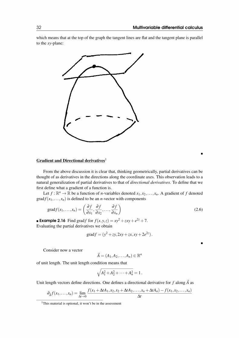
32 Multivariable differential calculus
which means that at the top of the graph the tangent lines are flat and the tangent plane is parallelto the xy-plane:
�
Gradient and Directional derivatives1
From the above discussion it is clear that, thinking geometrically, partial derivatives can bethought of as derivatives in the directions along the coordinate axes. This observation leads to anatural generalization of partial derivatives to that of directional derivatives. To define that wefirst define what a gradient of a function is.
Let f : Rn→ R be a function of n-variables denoted x1,x2, . . . ,xn. A gradient of f denotedgrad f (x1, . . . ,xn) is defined to be an n-vector with components
grad f (x1, . . . ,xn) =
(∂ f∂x1
,∂ f∂x2
, . . . ,∂ f∂xn
)(2.6)
� Example 2.16 Find grad f for f (x,y,z) = xy2 + zxy+ e2z +7.Evaluating the partial derivatives we obtain
grad f = (y2 + zy,2xy+ zx,xy+2e2z) .
�
Consider now a vector~A = (A1,A2, . . . ,An) ∈ Rn
of unit length. The unit length condition means that√A2
1 +A22 + · · ·+A2
n = 1 .
Unit length vectors define directions. One defines a directional derivative for f along ~A as
∂~A f (x1, . . . ,xn) = lim∆t→0
f (x1 +∆tA1,x2,x2 +∆tA2, . . . ,xn +∆tAn)− f (x1,x2, . . . ,xn)
∆t1This material is optional, it won’t be in the assessment
2.5 Higher order partial derivatives 33
We observe from this definition that when ~A is directed along one of the coordinate axes thisdefinition gives the partial derivative in the corresponding variable. More generally one can showthat
∂~A f (x1, . . . ,xn) = grad f ·~A = A1∂1 f +A2∂2 f + . . .An∂n f .
This means that directional derivatives can be evaluated as linear combinations of partial deriva-tives.
� Example 2.17 Let f (x,y) = 12 x4 + y3. Calculate the directional derivative along
~A =1√5(1,2) ∈ R2
at the point (−1,1) Since fx = 2x3, fy = 3y2 we have fx(−1,1) =−2, fy(−1,1) = 3 so that
∂~A f (−1,1) = A1 fx(−1,1)+A2 fy(−1,1) =1√5· (−2)+
2√5·3 =
4√5
�
We will not be using gradient and directional derivatives in the rest of this course. They willbe further discussed in the 3rd year Vector Analysis course (F19MV).
2.5 Higher order partial derivatives
If f : R2 → R, then ∂ f∂x is also a function of two variables. Thus we can consider its partial
derivatives
∂
∂x
(∂ f∂x
)=
∂ 2 f∂x2 = fxx ,
∂
∂y
(∂ f∂x
)=
∂ 2 f∂y∂x
= fxy , (2.7)
where we exhibited different notations used for these second order partial derivatives.Similarly we can consider
∂
∂x
(∂ f∂y
)=
∂ 2 f∂x∂y
= fyx ,∂
∂y
(∂ f∂y
)=
∂ 2 f∂y2 = fyy . (2.8)
� Example 2.18 For f (x,y) = x3−4xy2 we calculate
∂ f∂x
= 3x2−4y2 ,∂ f∂y
=−8xy ,∂ 2 f∂x2 = 6x ,
∂ 2 f∂y∂x
=−8y ,∂ 2 f
∂x∂y=−8y ,
∂ 2 f∂y2 =−8x .
�
Theorem 2.5.1 — The mixed derivatives theorem. Consider f : D→ R for some D⊂ R2.If fx, fy, fxy, fyx exist at any (x,y) ∈ D and moreover the functions fxy, fyx are continuous,then
fxy(x,y) = fyx(x,y) for any (x,y) ∈ D .
When the conditions of this theorem are violated the mixed derivatives can be different. Thishappens in the following example.
34 Multivariable differential calculus
� Example 2.19 Consider a function defined so that
f (x,y) = xyx2− y2
x2 + y2 for (x,y) 6= (0,0)
and f (0,0) = 0. We find
∂ f∂x
= y ·(
x2− y2
x2 + y2 +4x2y2
(x2 + y2)2
)for (x,y) 6= (0,0). To get the value fx(0,0), we use the general definition:
∂ f∂x
(0,0) = lim∆x→0
(∆x · y · ∆x2− y2
(∆x)2 + y2 −0)1
∆x
)∣∣∣y=0
= 0 .
Substituting in the first expression (x,y) = (0,y), we find
∂ f∂x
(0,y) =−y .
Furthermore, by definition,
∂ 2 f∂y∂x
(0,0) = lim∆y→0
(∂ f∂x
(0,∆y)− ∂ f∂x
(0,0)) 1
∆y=−1 .
Similarly,
∂ f∂y
= x(
x2− y2
x2 + y2 −4x2y2
(x2 + y2)2
)for (x,y) 6= (0,0). Also,
∂ f∂y
(x,0) = x and∂ 2 f
∂x∂y(0,0) = 1 .
Thus for this function,
∂ 2 f∂y∂x
(0,0) =−1 6= ∂ 2 f∂x∂y
(0,0) = 1 .
�
In this course we will predominantly deal with functions for which all derivatives are continuousin a given domain and thus the mixed derivatives will coincide.
R We can easily generalize the definition of higher derivatives to functions of any number ofvariables. The above theorem generalizes to higher order derivatives.
� Example 2.20 Let f : R→ R and let
u(x,y) = f(y
x
)+2xy
1. Show that
x ·ux + y ·uy = 4xy (2.9)
2.5 Higher order partial derivatives 35
2. Deduce that
x2 ·uxx +2xy ·uxy + y2 ·uyy = 4xy (2.10)
Solution First we calculate using chain rule
ux =−yx2 · f ′
(yx
)+2y , uy =
1x· f ′(y
x
)+2x .
Hence
x ·ux + y ·uy =−yx· f ′(y
x
)+2xy+
yx· f ′(y
x
)+2xy = 4xy ,
and this is what we had to show in part 1 of the problem.
To do part 2, we first differentiate formula (2.9) with respect to x. This gives
ux + xuxx + yuxy = 4y .
Hence multiplying this by x we obtain
xux + x2uxx + xyuxy = 4xy . (2.11)
Differentiating (2.9) with respect to y gives
xuyx +uy + yuyy = 4x .
Multiplying the last expression by y we obtain
xyuyx + yuy + y2uyy = 4xy .
Adding together the last equation and equation (2.11) we get
x2uxx +2xyuxy + y2uyy + xux + yuy = 8xy .
Using (2.9) in the last expression we finally obtain (2.10). �
� Example 2.21 For the function
f (x,y,z) =xyz
(y2 + z2)2 ,
find fyxzx away from the points with y = z = 0.
Solution By the mixed derivatives theorem 2.5.1,
fyxzx = fxxyz
in the region at hand. We calculate
fx =yz
(y2 + z2)2 , fxx = 0 .
Therefore,
fyxzx = 0 .
�
36 Multivariable differential calculus
� Example 2.22 Let f : R1→ R1 be a function of one variable. Consider the function h : R2→R1, defined in terms of f as
h(x,y) = f 3(x− y2) =[
f (x− y2)]3
.
Determine hx(x,y), hy(x,y) and hxy(x,y) in terms of f , the variables x and y, and in terms of thederivatives f ′ and f ′′.
Solution
hx = 3 f 2(x− y2) · ∂ f (x− y2)
∂x= 3 f 2(x− y2) · f ′(x− y2)
hy = 3 f 2(x− y2) · ∂ f (x− y2)
∂y= 3 f 2(x− y2) · f ′(x− y2) · (−2y)
hxy =∂
∂y
[3 f 2(x− y2) · f ′(x− y2)
]= 3 ·2 f (x− y2) · f ′(x− y2) · (−2y) · f ′(x− y2)+3 f 2(x− y2) · f ′′(x− y2) · (−2y) .
�
2.6 The chain rule and partial derivatives.Suppose f is a function of x and x is a function of u so that we have a composite functionh(u) = f (x(u)). Then the chain rule says that
dh(u)du
(u) =d f (x(u))
dx(x(u)) · dx(u)
du(u) . (2.12)
It is customary to shorten the notations in this equation to
dhdu
=d fdx· dx
du,
or even to the form
d fdu
=d fdx· dx
du.
Consider now a function f : R2→ R1 of two variables x and y, where x and y are each functionsof u and v. Let
h(u,v) := f (x(u,v),y(u,v))
dentote the composite function.
Theorem 2.6.1 If the functions d fdx and d f
dy are continuous, then
∂h(u,v)∂u
=∂ f∂x
(x(u,v),y(u,v)) · ∂x∂u
(u,v)+∂ f∂y
(x(u,v),y(u,v)) · ∂y∂u
(u,v) , (2.13)
or, for brevity,
∂h∂u
=∂ f∂x· ∂x
∂u+
∂ f∂y· ∂y
∂u.
2.6 The chain rule and partial derivatives. 37
By some abuse of notations, we can also write
∂ f∂u
=∂ f∂x· ∂x
∂u+
∂ f∂y· ∂y
∂u∂ f∂v
=∂ f∂x· ∂x
∂v+
∂ f∂y· ∂y
∂v.
(2.14)
The theorem easily generalizes to functions of more variables, e.g. for f (x,y,z) with x = x(u,v),y = y(u,v) and z = z(u,v), we have
∂ f∂u
=∂ f∂x· ∂x
∂u+
∂ f∂y· ∂y
∂u+
∂ f∂ z· ∂ z
∂u.
Note that the number of variables can change when we form a composite function. For example,for f (x,y) with x = x(u) and y = y(u), the composite function h(u) = f (x(u),y(u)) is a functionof one variable, with
dhdu
=∂ f∂x· ∂x
∂u+
∂ f∂y· ∂y
∂u.
As another example, consider f (x) with x = x(u,v), so that h(u,v) := f (x(u,v)) is a function oftwo variables, with
∂h∂u
=d fdx· ∂x
∂u,
∂h∂v
=d fdx· ∂x
∂v.
� Example 2.23 Let f (x,y) = x2 + y, x = u2 + v and y = v−u. Find ∂ f∂u
(i) by substitution, and(ii) by using the chain rule.
Solution
(i) f = (u2 + v)2 + v−u = u4 +2u2v+ v2 + v−u
⇒ ∂ f∂u
= 4u3 +4uv−1 .
(ii)∂ f∂u
=∂ f∂x· ∂x
∂u+
∂ f∂y· ∂y
∂u= 2x ·2u+1 · (−1)
= 4u(u2 + v)−1 .
Here, in the second to last line, we have inserted the explicit formula for x in terms of u and v inorder to obtain an answer expressed just in terms of these two variables. �
� Example 2.24 Let f be a function of x and y with x = u+ v and y = u · v. Find formulae for∂ f∂v and ∂ 2 f
∂u∂v in terms of the partial derivatives of f w.r.t. x and y.
38 Multivariable differential calculus
Solution
∂x∂u
= 1 ,∂x∂v
= 1 ,∂y∂u
= v ,∂y∂v
= u
⇒ ∂ f∂v
=∂ f∂x· ∂x
∂v+
∂ f∂y· ∂y
∂v=
∂ f∂x
+u · ∂ f∂y
∂ 2 f∂u∂v
=∂
∂u
[∂ f∂x
+u · ∂ f∂y
]=
∂
∂u
(∂ f∂x
)+
∂
∂u
(u · ∂ f
∂y
)=
∂
∂u
(∂ f∂x
)+u · ∂
∂u
(∂ f∂y
)+
∂ f∂y
.
Now, we may use the chain rule to evaluate the remaining partial derivatives w.r.t. u:
∂
∂u
(∂ f∂x
)=
∂
∂x
(∂ f∂x
)· ∂x
∂u+
∂
∂y
(∂ f∂x
)· ∂y
∂u=
∂ 2 f∂x2 + v · ∂ 2 f
∂y∂x∂
∂u
(∂ f∂y
)=
∂
∂x
(∂ f∂y
)· ∂x
∂u+
∂
∂y
(∂ f∂y
)· ∂y
∂u=
∂ 2 f∂x∂y
+ v · ∂2 f
∂y2 .
Therefore we finally obtain
∂ 2 f∂u∂v
=∂ 2 f∂x2 +uv · ∂
2 f∂y2 +(u+ v) · ∂ 2 f
∂x∂y+
∂ f∂y
.
�
2.7 Transforming equations.
Sometimes equations can be simplified by changing variables.
� Example 2.25 Consider an equation involving the partial derivatives of some functionw = w(x,y):
wx +wy = 0 .
Suppose that x = u+v and y = u−v. Transform the equation so that it is expressed in terms of uand v.
Solution
wx =∂w∂u· ∂u
∂x+
∂w∂v· ∂v
∂x, wy =
∂w∂u· ∂u
∂y+
∂w∂v· ∂v
∂y.
We have that u = (x+y)2 and v = (x−y)
2 , so
∂u∂x
=12,
∂u∂y
=12,
∂v∂x
=12,
∂v∂y
=−12.
Hence
wx =12
wu +12
wv , wy =12
wu−12
wv ,
2.7 Transforming equations. 39
so the equation becomes
wx +wy =12(wu +wv +wu−wv) = 0 ,
i.e. wu = 0 .
�

Implicit functions.Implicit differentiation.
More variablesFunctions f : Rn→ Rm
Total derivativesVarious theorems about total derivativesTaylor’s ExpansionTaylor’s formula in two dimensionsMore applications
3 — Applications of partial derivatives
3.1 Implicit functions.Definition 3.1.1 — C1-class function. A function f : Rn→ R is called a C1-class functionif all of its partial derivatives exist and are continuous.
Definition 3.1.2 — Solution function. Consider an equation of the form
f (x,y) = 0 . (3.1)
A solution of this equation is simply any pair of numbers, say, (a,b), for which f (a,b) = 0.We will say that a function y(x) is a solution function if f (x,y(x)) = 0 for all x ∈ Dy, whereDy denotes the domain of y(x). Similarly, we could have a solution function x(y) such thatf (x(y),y) = 0 for all y ∈ Dx, where Dx denotes the domain of x(y).
� Example 3.1 Consider the equation
x2 + y2 = 1 .
We can solve this equation for y as a function of x, and we find two solution functions:
y =√
1− x2 , y =−√
1− x2 , −1≤ x≤ 1 .
We could also solve for x as a function of y, resulting in
x =√
1− y2 , x =−√
1− y2 , −1≤ y≤ 1 .
�
In principle, there is nothing special about which variable we solve for, but in practice itmight be much easier to solve for one variable rather than the other.
� Example 3.2 The equation
y− x− 12
siny = 0
can be easily solved for x(y) = y− 12 siny, but cannot be solved explicitly for y(x). �
42 Applications of partial derivatives
Very often, we cannot solve explicitly for either variable.
� Example 3.3 The equation
ln√
x2 + y2 = tan−1(y
x
)cannot be solved explicitly for either variable. �
In general, any equation of the form f (x,y) = 0 is said to define its solution functionsimplicitly (if they exist).
3.2 Implicit differentiation.Suppose y(x) is a solution function for f (x,y) = 0. We can calculate the derivative dy
dx usingpartial derivatives and the chain rule. Differentiating f (x,y(x)) = 0 with respect to x, we obtain
∂ f∂x
+∂ f∂y· ∂y
∂x= 0 ,
hence
dydx
=− fx
fy. (3.2)
This formula is called the implicit differentiation formula.
� Example 3.4 Let us find dydx for y =
√1− x2 from Example 3.1 (with f (x,y) = x2 +y2−1) by
(i) explicit differentiation, and by(ii) using the implicit differentiation formula.
Solution
(i)ddx
√1− x2 =− x√
1− x2
(ii)dydx
=− fx
fy=−2x
2y=− x√
1− x2,
where in the last step we substituted y =√
1− x2. �
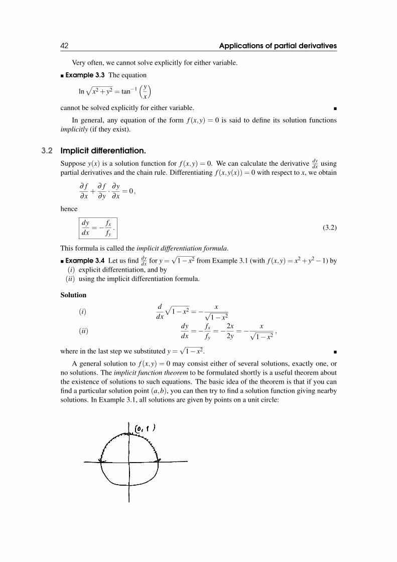
A general solution to f (x,y) = 0 may consist either of several solutions, exactly one, orno solutions. The implicit function theorem to be formulated shortly is a useful theorem aboutthe existence of solutions to such equations. The basic idea of the theorem is that if you canfind a particular solution point (a,b), you can then try to find a solution function giving nearbysolutions. In Example 3.1, all solutions are given by points on a unit circle:
3.2 Implicit differentiation. 43
The solution y =√
1− x2 with −1≤ x≤ 1 covers the upper semi-circle – in the graphics above,the solution point (0,1) is marked as an example. The other solution, y = −
√1− x2 with
−1≤ x≤ 1, covers the lower semi-circle. Note in particular that the lower semi-circle does notinclude the point (0,1).
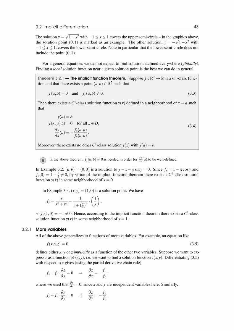
For a general equation, we cannot expect to find solutions defined everywhere (globally).Finding a local solution function near a given solution point is the best we can do in general.
Theorem 3.2.1 — The implicit function theorem. Suppose f : R2→ R is a C1-class func-tion and that there exists a point (a,b) ∈ R2 such that
f (a,b) = 0 and fy(a,b) 6= 0 . (3.3)
Then there exists a C1-class solution function y(x) defined in a neighborhood of x = a suchthat
y(a) = b
f (x,y(x)) = 0 for all x ∈ Dy
dydx
(a) =− fx(a,b)fy(a,b)
.
(3.4)
Moreover, there exists no other C1-class solution y(x) with y(a) = b.
R In the above theorem, fy(a,b) 6= 0 is needed in order for dydx (a) to be well-defined.
In Example 3.2, (a,b) = (0,0) is a solution to y− x− 12 siny = 0. Since fy = 1− 1
2 cosy andfy(0) = 1− 1
2 6= 0, by virtue of the implicit function theorem there exists a C1-class solutionfunction y(x) in some neighborhood of x = 0.
In Example 3.3, (x,y) = (1,0) is a solution point. We have
fy =y
x2 + y2 −1
1+( y
x
)2 ·(
1x
),
so fy(1,0) =−1 6= 0. Hence, according to the implicit function theorem there exists a C1-classsolution function y(x) in some neighborhood of x = 1.
3.2.1 More variablesAll of the above generalizes to functions of more variables. For example, an equation like
f (x,y,z) = 0 (3.5)
defines either x, y or z implicitly as a function of the other two variables. Suppose we want to ex-press z as a function of (x,y), i.e. we want to find a solution function z(x,y). Differentiating (3.5)with respect to x gives (using the partial derivative chain rule)
fx + fz ·∂ z∂x
= 0 ⇒ ∂ z∂x
=− fx
fz,
where we used that ∂y∂x = 0, since x and y are independent variables here. Similarly,
fy + fz ·∂ z∂y
= 0 ⇒ ∂ z∂y
=−fy
fz.
44 Applications of partial derivatives
� Example 3.5 Suppose z is defined implicitly by
z2 + y7 +5zy
x2 +1= x .
Find ∂ z∂x and ∂ z
∂y .
Solution
f (x,y,z) = z2 + y7 +5zy
x2 +1− x
⇒ ∂ z∂x
=−
(− 5zy
(x2+1)2 · (2x)−1)
(2z+ 5y
x2+1
) ,∂ z∂y
=−
(7y6 + 5z
x2+1
)(
2z+ 5yx2+1
) .
�
Theorem 3.2.2 — The implicit function theorem (3-variable case).Suppose that f : R3→ R has partial derivatives and that there exists a point (x,y,z) = (a,b,c)such that
f (a,b,c) = 0 and fz(a,b,c) 6= 0 . (3.6)
Then there exists a solution function z(x,y) defined near (x,y) = (a,b) such that:
z(a,b) = c
f (x,y,z(x,y)) = 0∂ z∂x
(a,b) =− fx(a,b,c)fz(a,b,c)
,∂ z∂y
=−fy(a,b,c)fz(a,b,c)
,
(3.7)
and there exists no other differentiable solution function z(x,y) with z(a,b) = c.
� Example 3.6 Consider the equation
z2 +2yx+ zx = 0 .
(i) Does the implicit function theorem apply, and can we solve for z = z(x,y) near the points(a) z = 1 , x = 1 y =−1(b) z = 1 , x = 2 , y =−1
4 ?(ii) At the second particular solution (b), can one obtain a solution function for y = y(x,z)?
Solution (i) We compute fz = 2z+ x and find that
fz(1,−1,1) = 2+1 = 3 6= 0 ,
so a solution function z(x,y) exists near this solution point. On the other hand,
fz(−2,−14,1) = 2−2 = 0 ,
so the implicit function theorem is not applicable in this case and there exists no solution functionz(x,y) near this solution point.
3.2 Implicit differentiation. 45
(ii) We compute that with fy = 2x,
fy(−2,−14,1) =−4 6= 0 ,
so there exists a solution function y = y(x,z) near that particular solution point. �
Let us now look at a pair of equations:{f (x,y,z) = 0g(x,y,z) = 0
. (3.8)
Since there are two equations, we expect that these equations implicitly define, say, (x,y) as afunction of z, i.e. we expect to find solution functions (x(z),y(z)) (there may be several or nosolution functions, depending on the particular equations). Differentiating (3.8) w.r.t. z gives
fx ·dxdz
+ fy ·dydz
+ fz = 0
gx ·dxdz
+gy ·dydz
+gz = 0. (3.9)
This is a pair of simultaneous linear equations for dxdz and dy
dz . Using a matrix notation, the solutionto this system may be written as(
dxdzdydz
)=−
(fx fy
gx gy
)−1( fz
gz
),
where (. . .)−1 denotes the matrix inverse as usual. This matrix equation suggests that thederivative condition for the solution function to exist should be that the matrix(
fx fy
gx gy
)is invertible. Equivalently,
det(
fx fy
gx gy
)= fx ·gy− fy ·gx
should be non-vanishing. The precise statement is given in the following theorem.
Theorem 3.2.3 Let f : R3→ R, g : R3→ R be two C1-class functions and let (a,b,c) ∈ R3
be a point such that f (a,b,c) = 0 and g(a,b,c) = 0. If
det(
fx fy
gx gy
)= fx ·gy− fy ·gx 6= 0 , (3.10)
then there exists a C1-class solution function (x(z),y(z)) in a neighborhood of z = c and suchthat (x(c),y(c)) = (a,b).
� Example 3.7 Consider a pair of equations{f (x,y,z) = x · siny+ yz+ z3 = 0g(x,y,z) = x+ ex·y− yz2 = 0
.
What does the implicit function theorem say about the existence of C1-class solution functionsx(z) and y(z) near (x,y,z) = (−1,0,0)?
46 Applications of partial derivatives
Solution (fx fy
gx gy
)(−1,0,0) =
(siny (xcosy+ z)
(1+ yex·y) (xex·y− z2)
)∣∣∣∣(−1,0,0)
=
(0 −11 −2
)⇒ det
(fx fy
gx gy
)(−1,0,0) = det
(0 −11 −1
)= 1 6= 0 .
Thus, the matrix is invertible and by virtue of the implicit function theorem, there exists aC1-class solution function (x(z),y(z)) near z = 0. �
3.3 Functions f : Rn→ Rm
Up to now we have talked about functions f : Rn→ R, i.e. we put in n numbers (x1, . . . ,xn) andget back a singe number f (x1, . . . ,xn). To save space we will often write
x = (x1, . . . ,xn) ∈ Rn (3.11)
and write f (x) ∈ R. To use this notation, we need to keep track of whether x is a point in Rn or anumber in R. We will often write x ∈ Rn for general theorems and (x,y) ∈ R2 or (x,y,z) ∈ R3 inparticular examples. We will also use the notation
‖v‖ :=√
v21 + v2
2 + . . .+ v2n (3.12)
for any vector v = (v1, . . . ,vn) ∈ Rn, which is the length of v. Generalizing f : Rn→ R, we canconsider a function which gives us back m numbers, which we can write as
f (x) = f (x1, . . . ,xn) = ( f1(x), . . . , fm(x)) ∈ Rm . (3.13)
This means that we have a function f : Rn→ Rm, i.e. a function from Rn to Rm. Note that eachof the functions f1, . . . , fm is a function with values in R, that is fi : Rn→ R. Hence, a functionf : Rn→ Rm is simply a collection of m real-valued functions bracketed together.
Sometimes it is convenient to write f : Rn→ Rm as
f (x) =
f1(x)...
fm(x)
, (3.14)
since this works better when we have matrix operations at hand.
3.4 Total derivativesDespite appearances, partial derivatives are not the exact counterparts of the derivative of afunction of one variable. Recall the definition of the derivative in the one variable case: Iff : R→ R, the derivative at a point x = a is defined as
f ′(a) := limh→0
f (a+h)− f (a)h
. (3.15)
The function f is differentiable at x = a if the limit exists. This is equivalent to
limh→0
∣∣∣∣ f (a+h)− f (a)−h f ′(a)h
∣∣∣∣= 0 , (3.16)
3.4 Total derivatives 47
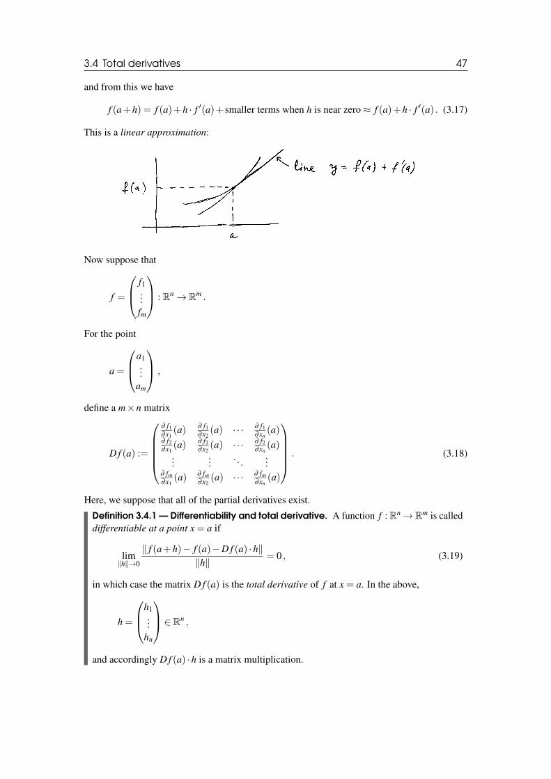
and from this we have
f (a+h) = f (a)+h · f ′(a)+ smaller terms when h is near zero≈ f (a)+h · f ′(a) . (3.17)
This is a linear approximation:
Now suppose that
f =
f1...fm
: Rn→ Rm .
For the point
a =
a1...
am
,
define a m×n matrix
D f (a) :=
∂ f1∂x1
(a) ∂ f1∂x2
(a) · · · ∂ f1∂xn
(a)∂ f2∂x1
(a) ∂ f2∂x2
(a) · · · ∂ f2∂xn
(a)...
.... . .
...∂ fm∂x1
(a) ∂ fm∂x2
(a) · · · ∂ fm∂xn
(a)
. (3.18)
Here, we suppose that all of the partial derivatives exist.
Definition 3.4.1 — Differentiability and total derivative. A function f :Rn→Rm is calleddifferentiable at a point x = a if
lim‖h‖→0
‖ f (a+h)− f (a)−D f (a) ·h‖‖h‖
= 0 , (3.19)
in which case the matrix D f (a) is the total derivative of f at x = a. In the above,
h =
h1...
hn
∈ Rn ,
and accordingly D f (a) ·h is a matrix multiplication.
48 Applications of partial derivatives
Definition 3.4.2 A function f : Rn→ Rm is differentiable if it is differentiable at each pointof its domain.
Theorem 3.4.1 If a function f : Rn→ Rm has derivatives
∂ fi
∂x ji = 1, . . . ,m , j = 1, . . . ,n
and if all ∂ fi∂x j
are continuous functions at x = a, then f is differentiable at x = a.
Definition 3.4.3 If f and all derivatives ∂ fi∂x j
are continuous on the whole domain, then f is in
C1. Here, the superscript 1 stands for the first derivative of f .
� Example 3.8
f (x,y) =x2y
x2 + y2 for (x,y) 6= (0,0)
f (0,0) = 0 .
One can compute that ∂ f∂x (0,0) =
∂ f∂y (0,0) = 0 both exist, but the function is not differentiable at
(x,y) = (0,0). �
� Example 3.9 Consider the function f : R2→ R2 defined by
f1(x,y) = x2 +5y+ xy
f2(x,y) = 3xy+ y3 .
Calculate the total derivative.
Solution We have
∂ f1
∂x= 2x+ y ,
∂ f1
∂y= 5+ x ,
∂ f2
∂x= 3y ,
∂ f2
∂y= 3x+3y2 .
All these functions are polynomials and are therefore continuous, which implies that f isdifferentiable, with first derivative
D f (x,y) =((2x+ y) (5+ x)
3y (3x+3yz)
).
�
� Example 3.10 For f : R2→ R defined by
f (x,y) =xy
(y 6= 0) ,
show that f is differentiable at (x,y) = (1,2) and find D f (1,2).
Solution
∂ f∂x
=1y,
∂ f∂y
=− xy2 .
3.5 Various theorems about total derivatives 49
These are continuous at (x,y) = (1,2), hence f is differentiable at this point, with
D f (1,2) =(1
2 −14
).
�
� Example 3.11 Calculate the total derivative D f (1,1) for
f =
x2 +5yex · y
y · lnx
: R2→ R3 .
Solution We have
D f (1,1) =
2x 5ex · y ex
yx lnx
(1,1) =
2 5e e1 0
.
�
3.5 Various theorems about total derivativesTheorem 3.5.1 — Chain rule. If g : Rn → Rm is differentiable at a point a ∈ Rn, and iff :Rm→R` is differentiable at the point g(x) ∈Rm, then h = f ◦g :Rn→R` is differentiableat the point a, with
Dh(a) = D( f ◦g)(a) = D f (g(a)) ·Dg(a) , (3.20)
where the symbol · denotes the matrix product as usual.
� Example 3.12 Suppose that we are given two functions g : R2→ R2 and f : R2→ R, and let(a,b) ∈R2 be a point. Let f depend on (x,y), and let g depend on (u,v). Consider the compositefunction h(u,v) = f (g(u,v)),
h : R2 g−→ R2 f−→ R .
Then we have
Dh(a,b) =(
∂h∂u
∂h∂v
)∣∣∣∣(u,v)=(a,b)
= D f ·Dg(a,b)
=(
∂ f∂x
∂ f∂y
)∣∣∣∣(x,y)=g(a,b)
·
(∂g1∂u
∂g1∂v
∂g2∂u
∂g2∂v
)∣∣∣∣(u,v)=(a,b)
.
Writing explicitly x = g1(u,v) and y = g2(u,v), and consequently(∂g1∂u
∂g1∂v
∂g2∂u
∂g2∂v
)=
(∂x∂u
∂x∂v
∂y∂u
∂y∂v
),
we obtain
∂h∂u
=∂ f∂x· ∂x
∂u+
∂ f∂y· ∂y
∂u,
∂h∂v
=∂ f∂x· ∂x
∂v+
∂ f∂y· ∂y
∂v.
Thus the chain rule we looked at before (Theorem 2.6.1) is a special case of the above generalchain rule. �
50 Applications of partial derivatives
Consider next a set of implicit equations:f1(x1, . . . ,xm,y1, . . . ,yn) = 0
...fn(x1, . . . ,xm,y1, . . . ,yn) = 0
. (3.21)
Here, we have n equations in m+n variables. So we expect to be able to solve them for n ofthe unknowns, say (without loss of generality) y1, . . . ,yn (that is why we are using two differentletters to label the m+n variables in the above equation system). We will write for brevity
x = (x1, . . . ,xm) ∈ Rm , y = (y1, . . . ,yn) ∈ Rn , (3.22)
so (x,y) ∈ Rm+n and
f (x,y) =
f1(x,y)...
fn(x,y)
. (3.23)
We also write
Dy f (x,y) =
∂ f1∂y1
· · · ∂ f1∂yn
......
∂ fn∂y1
· · · ∂ fn∂yn
. (3.24)
Theorem 3.5.2 — The implicit function theorem (general version). Suppose that f is C1
and that f (a,b) = 0 for some point (a,b) ∈Rm+n (with a ∈Rm, b ∈Rn). Suppose further thatthe matrix Dy f (a,b) is invertible. Then there exists a C1 solution function y(x) : Rm→ Rn
defined for x ∈ Rm close to a and such that
y(a) = b , f (x,y(x)) = 0 .
R The invertibility of Dy f (a,b) is equivalent to
detDy f (a,b) 6= 0 .
� Example 3.13 Consider the case of two equations for three variables:
u2 +uv−w− vw = 0
u+u2v+ v2w−3 = 0 .
Consider the solution point (u,v,w) = (1,1,1). Use the implicit function theorem to determinewhether there exists a C1-class solution function (u(w),v(w)) in the neighborhood of the solutionpoint (1,1,1).
Solution We compute
Du,v f (1,1,1) =
(∂ f1∂u
∂ f1∂v
∂ f2∂u
∂ f2∂v
)∣∣∣∣(1,1,1)
=
((2u+ v) (u−w)(2uv+1) (u2 +2vw)
)∣∣∣∣(1,1,1)
=
(3 03 3
).
Hence detDu,v f (1,1,1) = 9 6= 0 and there exists a solution function (u(w),v(w)) of C1-class ina neighborhood of w = 1. �
3.6 Taylor’s Expansion 51
3.6 Taylor’s ExpansionConsider f :R1→R1 such that at a given point x= x0 there exist f (x0), f ′(x0), f ′′(x0), . . . , f (n)(x0).We can construct an n-th degree polynomial pn(x) such that
pn(x0) = f (x0) , p′n(x0) = f ′(x0) , . . . , p(n)n (x0) = f (n)(x0) . (3.25)
It is convenient to write
pn(x) = c0 + c1(x− x0)+ c2(x− x0)2 + . . .+ cn(x− x0)
n . (3.26)
Then, if we set c0 = f (x0), pn(x0) = f (x0) is satisfied. We further calculate
p′n(x0) = c1 = f ′(x0)
p′′n(x0) = 2c2 = f ′′(x0) ⇒ c2 =f ′′(x0)
2!
p′′′n (x0) = 3 ·2 · c3 = 3!c3 = f ′′′(x0) ⇒ c3 =f ′′′(x0)
3!...
p(n)n (x0) = n · (n−1) · . . . ·2 ·1 · cn = n!cn = f (n)(x0) ⇒ cn =f (n)(x0)
n!.
(3.27)
Thus
pn(x) = f (x0)+(x− x0) f ′(x0)+(x− x0)
2
2!f ′′(x0)+ . . .+
(x− x0)n
n!f (n)(x− x0) . (3.28)
It turns out that such poynomials can serve as approximations of a given function f (x) in theneighborhood (i.e. near) a given point x0 where all the derivatives involved exist.
In general, we write
f (x) = pn(x)+ rn+1(x) , (3.29)
where
pn(x) =
tangent line equation︷ ︸︸ ︷f (x0)+(x− x0) f ′(x0)+ . . .+
(x− x0)n
n!f (n)(x0) (3.30)
is the nth degree Taylor polynomial centered at x0, and rn+1 is the difference between f (x) andpn(x), the so called remainder term.
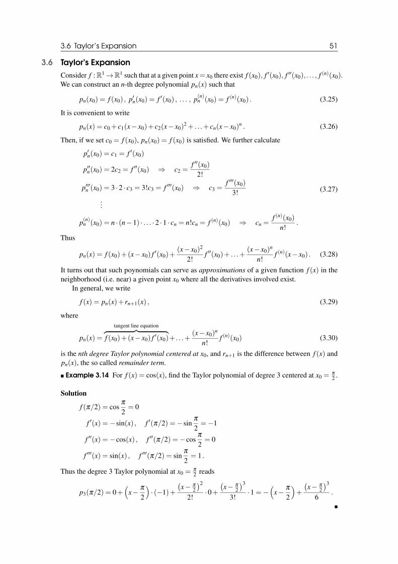
� Example 3.14 For f (x) = cos(x), find the Taylor polynomial of degree 3 centered at x0 =π
2 .
Solution
f (π/2) = cosπ
2= 0
f ′(x) =−sin(x) , f ′(π/2) =−sinπ
2=−1
f ′′(x) =−cos(x) , f ′′(π/2) =−cosπ
2= 0
f ′′′(x) = sin(x) , f ′′′(π/2) = sinπ
2= 1 .
Thus the degree 3 Taylor polynomial at x0 =π
2 reads
p3(π/2) = 0+(
x− π
2
)· (−1)+
(x− π
2
)2
2!·0+
(x− π
2
)3
3!·1 =−
(x− π
2
)+
(x− π
2
)3
6.
�
52 Applications of partial derivatives
If pn(x) is a good approximation, we expect that rn+1(x) is small when x is sufficiently closeto x0, i.e. when | x− x0 | is small enough. A quantitative expression of this heuristic idea is givenby the following theorem:
Theorem 3.6.1 — nth mean value theorem. For f : R1→ R1 such that f , f ′, . . . , f (n) arecontinuos at x = x0, the following formula holds:
f (x) = pn−1(x)+ rn(x) , (3.31)
where pn−1(x) denotes the Taylor polynomial of degree n−1 centered at x0, where
rn(x) =1n!(x− x0)
n f (n)(x∗) , (3.32)
and where x∗ is some point between x and x0,
x∗ = x0 +θ(x− x0) , 0≤ θ ≤ 1 .
If we know that the values of the nth order derivative on the interval between x0 and x arebounded by a certain constant, i.e. | f (n)(y)| ≤M, then
|rn(x)| ≤|x− x0|n
n!·M . (3.33)
3.6 Taylor’s Expansion 53
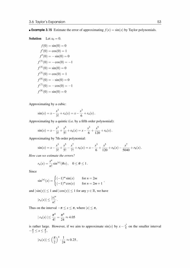
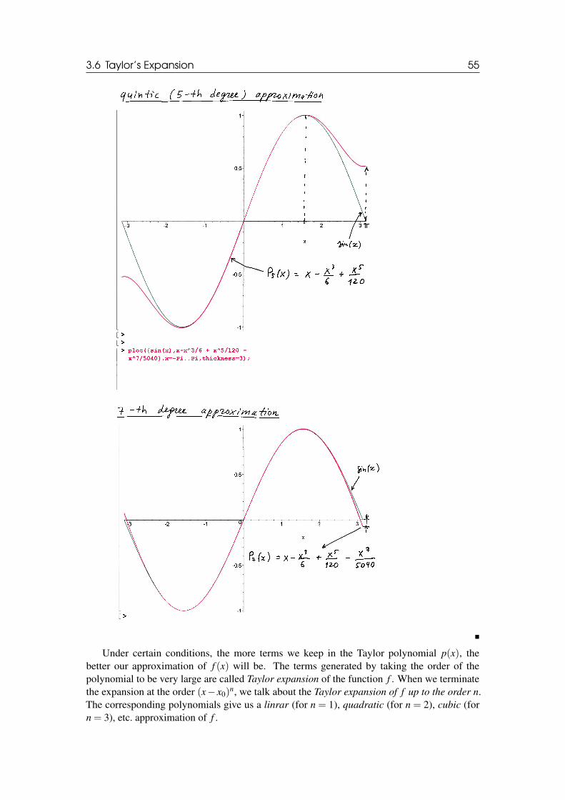
� Example 3.15 Estimate the error of approximating f (x) = sin(x) by Taylor polynomials.
Solution Let x0 = 0.
f (0) = sin(0) = 0
f ′(0) = cos(0) = 1
f ′′(0) =−sin(0) = 0
f (3)(0) =−cos(0) =−1
f (4)(0) = sin(0) = 0
f (5)(0) = cos(0) = 1
f (6)(0) =−sin(0) = 0
f (7)(0) =−cos(0) =−1
f (8)(0) = sin(0) = 0
Approximating by a cubic:
sin(x) = x− x3
3!+ r4(x) = x− x3
6+ r4(x) .
Approximating by a quintic (i.e. by a fifth order polynomial):
sin(x) = x− x3
3!+
x5
5!+ r6(x) = x− x3
6+
x5
120+ r6(x) .
Approximating by 7th order polynomial:
sin(x) = x− x3
3!+
x5
5!− x7
7!+ r8(x) = x− x3
6+
x5
120+ r6(x)−
x7
5040+ r8(x) .
How can we estimate the errors?
rn(x) =xn
n!sin(n)(θx) , 0≤ θ ≤ 1 .
Since
sin(n)(x) =
{(−1)m sin(x) for n = 2m(−1)m cos(x) for n = 2m+1
,
and |sin(y)| ≤ 1 and |cos(y)| ≤ 1 for any y ∈ R, we have
|rn(x)| ≤|x|n
n!.
Thus on the interval −π ≤ x≤ π , where |x| ≤ π ,
| r4(x) |≤π4
4!=
π4
24≈ 4.05
is rather large. However, if we aim to approximate sin(x) by x− x3
6 on the smaller interval−π
2 ≤ x≤ π
2 ,
|r4(x)| ≤(
π
2
)4· 1
24≈ 0.25 ,
54 Applications of partial derivatives
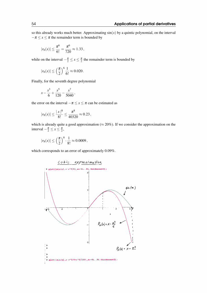
so this already works much better. Approximating sin(x) by a quintic polynomial, on the interval−π ≤ x≤ π the remainder term is bounded by
|r6(x)| ≤π6
6!=
π6
720≈ 1.33 ,
while on the interval −π
2 ≤ x≤ π
2 the remainder term is bounded by
|r6(x)| ≤(
π
2
)6 16!≈ 0.020 .
Finally, for the seventh degree polynomial
x− x3
6+
x5
120− x7
5040,
the error on the interval −π ≤ x≤ π can be estimated as
|r8(x)| ≤| x |8
8!≤ π8
40320≈ 0.23 ,
which is already quite a good approximation (≈ 20%). If we consider the approximation on theinterval −π
2 ≤ x≤ π
2 ,
|r8(x)| ≤(
π
2
)8· 1
8!≈ 0.0009 ,
which corresponds to an error of approximately 0.09%.
3.6 Taylor’s Expansion 55
�
Under certain conditions, the more terms we keep in the Taylor polynomial p(x), thebetter our approximation of f (x) will be. The terms generated by taking the order of thepolynomial to be very large are called Taylor expansion of the function f . When we terminatethe expansion at the order (x− x0)
n, we talk about the Taylor expansion of f up to the order n.The corresponding polynomials give us a linrar (for n = 1), quadratic (for n = 2), cubic (forn = 3), etc. approximation of f .
56 Applications of partial derivatives
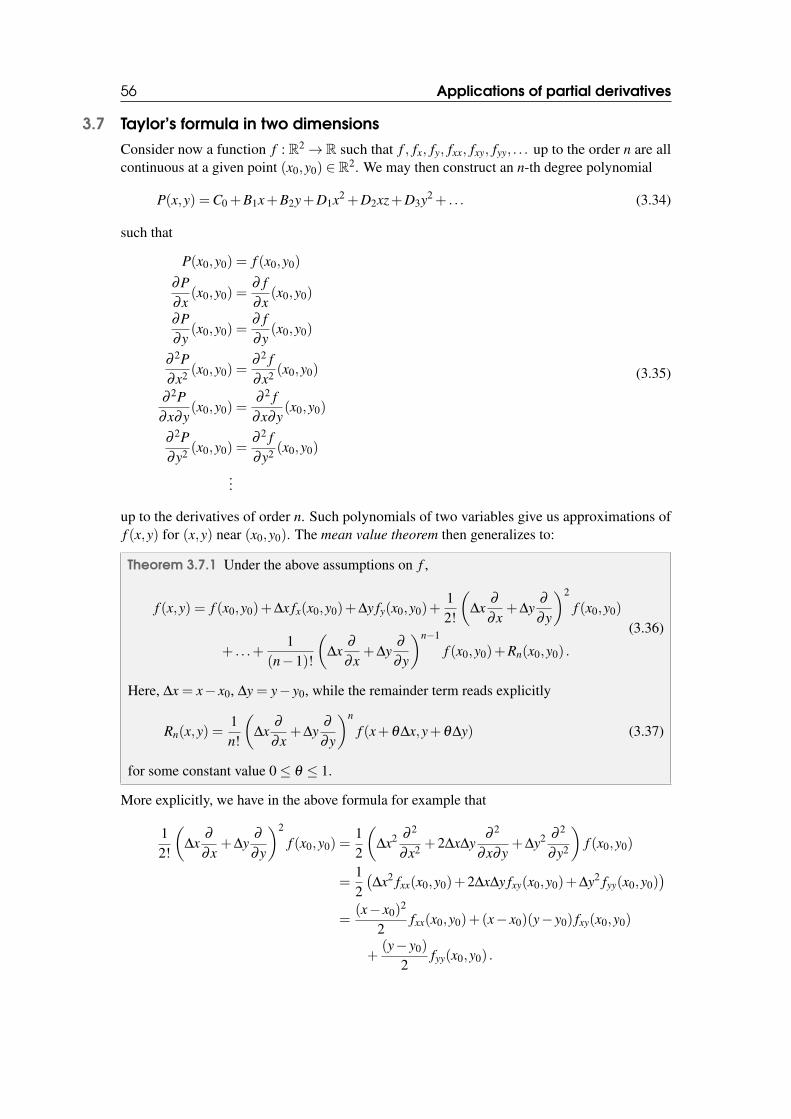
3.7 Taylor’s formula in two dimensionsConsider now a function f : R2→ R such that f , fx, fy, fxx, fxy, fyy, . . . up to the order n are allcontinuous at a given point (x0,y0) ∈ R2. We may then construct an n-th degree polynomial
P(x,y) =C0 +B1x+B2y+D1x2 +D2xz+D3y2 + . . . (3.34)
such that
P(x0,y0) = f (x0,y0)
∂P∂x
(x0,y0) =∂ f∂x
(x0,y0)
∂P∂y
(x0,y0) =∂ f∂y
(x0,y0)
∂ 2P∂x2 (x0,y0) =
∂ 2 f∂x2 (x0,y0)
∂ 2P∂x∂y
(x0,y0) =∂ 2 f
∂x∂y(x0,y0)
∂ 2P∂y2 (x0,y0) =
∂ 2 f∂y2 (x0,y0)
...
(3.35)
up to the derivatives of order n. Such polynomials of two variables give us approximations off (x,y) for (x,y) near (x0,y0). The mean value theorem then generalizes to:
Theorem 3.7.1 Under the above assumptions on f ,
f (x,y) = f (x0,y0)+∆x fx(x0,y0)+∆y fy(x0,y0)+12!
(∆x
∂
∂x+∆y
∂
∂y
)2
f (x0,y0)
+ . . .+1
(n−1)!
(∆x
∂
∂x+∆y
∂
∂y
)n−1
f (x0,y0)+Rn(x0,y0) .
(3.36)
Here, ∆x = x− x0, ∆y = y− y0, while the remainder term reads explicitly
Rn(x,y) =1n!
(∆x
∂
∂x+∆y
∂
∂y
)n
f (x+θ∆x,y+θ∆y) (3.37)
for some constant value 0≤ θ ≤ 1.
More explicitly, we have in the above formula for example that
12!
(∆x
∂
∂x+∆y
∂
∂y
)2
f (x0,y0) =12
(∆x2 ∂ 2
∂x2 +2∆x∆y∂ 2
∂x∂y+∆y2 ∂ 2
∂y2
)f (x0,y0)
=12(∆x2 fxx(x0,y0)+2∆x∆y fxy(x0,y0)+∆y2 fyy(x0,y0)
)=
(x− x0)2
2fxx(x0,y0)+(x− x0)(y− y0) fxy(x0,y0)
+(y− y0)
2fyy(x0,y0) .
3.8 More applications 57
� Example 3.16 Consider the function f (x,y) = ln(x+ y2
)in the vicinity of the point (x0,y0) =
(1,1):
f (1,1) = ln2
fx(x,y) =1
x+ y2 , fx(1,1) =12
fy(x,y) =2y
x+ y2 , fy(1,1) = 1 .
Thus, the linear approximation reads
f (x,y)≈ ln2+12(x−1)+1 · (y−1) =
x2+ y+
(ln2− 3
2
)fxx(x,y) =−
1(x+ y2)2 , fx(1,1) =−
14
fyy(x,y) = 2 · x− y2
(x+ y2)2 , fy(1,1) = 0
fxy(x,y) =−2y
(x+ y2)2 , fxy(1,1) =−12.
The quadratic approximation reads
f (x,y)≈ ln2+(x−1)
2+(y−1)+
12
[−(x−1)2
4+2 · (x−1)(y−1) ·
(−1
2
)]= ln2+
(x−1)2
+(y−1)− (x−1)2
8− 1
2(x−1)(y−1) .
�
Taylor expansions tend to give reasonable approximations of a given function f (x,y) nearthe expansion point (x0,y0), but they get worse as x, y move away from (x0,y0). The remainderterm Rn(x,y) can be used to estimate how good the approximation is.
3.8 More applicationsMore applications of partial derivatives (finding maxima and minima) will be discussed in thelast chapter of the notes. This is done so that the order of the material presented in the typednotes is the same as the order in which they appear in the lectures.

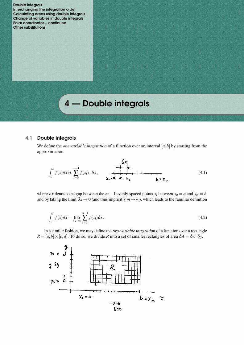
Double integralsInterchanging the integration orderCalculating areas using double integralsChange of variables in double integralsPolar coordinates – continuedOther substitutions
4 — Double integrals
4.1 Double integrals
We define the one variable integration of a function over an interval [a,b] by starting from theapproximation
∫ b
af (x)dx≈
m−1
∑i=0
f (xi) ·δx , (4.1)
where δx denotes the gap between the m+1 evenly spaced points xi between x0 = a and xm = b,and by taking the limit δx→ 0 (and thus implicitly m→∞), which leads to the familiar definition
∫ b
af (x)dx = lim
δx→0
m−1
∑i=0
f (xi)δx . (4.2)
In a similar fashion, we may define the two-variable integration of a function over a rectangleR = [a,b]× [c,d]. To do so, we divide R into a set of smaller rectangles of area δA = δx ·δy.
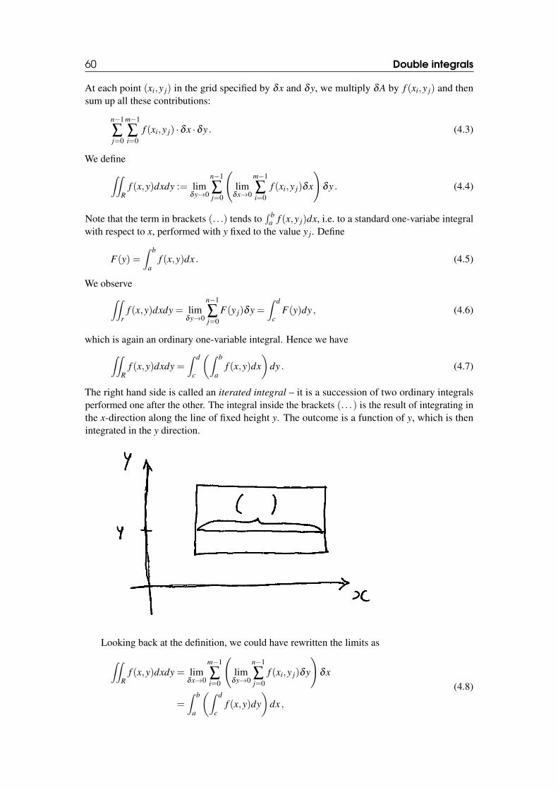
60 Double integrals
At each point (xi,y j) in the grid specified by δx and δy, we multiply δA by f (xi,y j) and thensum up all these contributions:
n−1
∑j=0
m−1
∑i=0
f (xi,y j) ·δx ·δy . (4.3)
We define∫∫R
f (x,y)dxdy := limδy→0
n−1
∑j=0
(lim
δx→0
m−1
∑i=0
f (xi,y j)δx
)δy . (4.4)
Note that the term in brackets (. . .) tends to∫ b
a f (x,y j)dx, i.e. to a standard one-variabe integralwith respect to x, performed with y fixed to the value y j. Define
F(y) =∫ b
af (x,y)dx . (4.5)
We observe∫∫r
f (x,y)dxdy = limδy→0
n−1
∑j=0
F(y j)δy =∫ d
cF(y)dy , (4.6)
which is again an ordinary one-variable integral. Hence we have∫∫R
f (x,y)dxdy =∫ d
c
(∫ b
af (x,y)dx
)dy . (4.7)
The right hand side is called an iterated integral – it is a succession of two ordinary integralsperformed one after the other. The integral inside the brackets (. . .) is the result of integrating inthe x-direction along the line of fixed height y. The outcome is a function of y, which is thenintegrated in the y direction.
Looking back at the definition, we could have rewritten the limits as∫∫R
f (x,y)dxdy = limδx→0
m−1
∑i=0
(lim
δy→0
n−1
∑j=0
f (xi,y j)δy
)δx
=∫ b
a
(∫ d
cf (x,y)dy
)dx ,
(4.8)
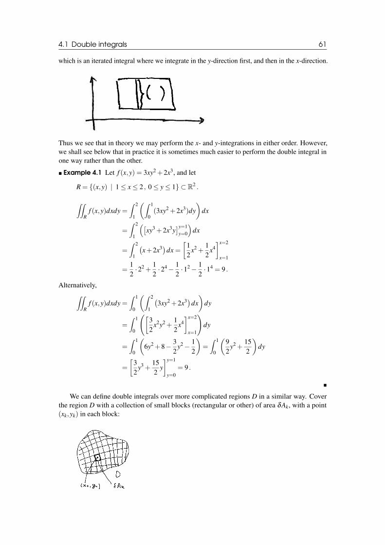
4.1 Double integrals 61
which is an iterated integral where we integrate in the y-direction first, and then in the x-direction.
Thus we see that in theory we may perform the x- and y-integrations in either order. However,we shall see below that in practice it is sometimes much easier to perform the double integral inone way rather than the other.
� Example 4.1 Let f (x,y) = 3xy2 +2x3, and let
R = {(x,y) | 1≤ x≤ 2 , 0≤ y≤ 1} ⊂ R2 .
∫∫R
f (x,y)dxdy =∫ 2
1
(∫ 1
0(3xy2 +2x3)dy
)dx
=∫ 2
1
([xy3 +2x3y
]y=1y=0
)dx
=∫ 2
1
(x+2x3)dx =
[12
x2 +12
x4]x=2
x=1
=12·22 +
12·24− 1
2·12− 1
2·14 = 9 .
Alternatively,∫∫R
f (x,y)dxdy =∫ 1
0
(∫ 2
1
(3xy2 +2x3)dx
)dy
=∫ 1
0
([32
x2y2 +12
x4]x=2
x=1
)dy
=∫ 1
0
(6y2 +8− 3
2y2− 1
2
)=∫ 1
0
(92
y2 +152
)dy
=
[32
y3 +152
y]y=1
y=0= 9 .
�
We can define double integrals over more complicated regions D in a similar way. Coverthe region D with a collection of small blocks (rectangular or other) of area δAk, with a point(xk,yk) in each block:
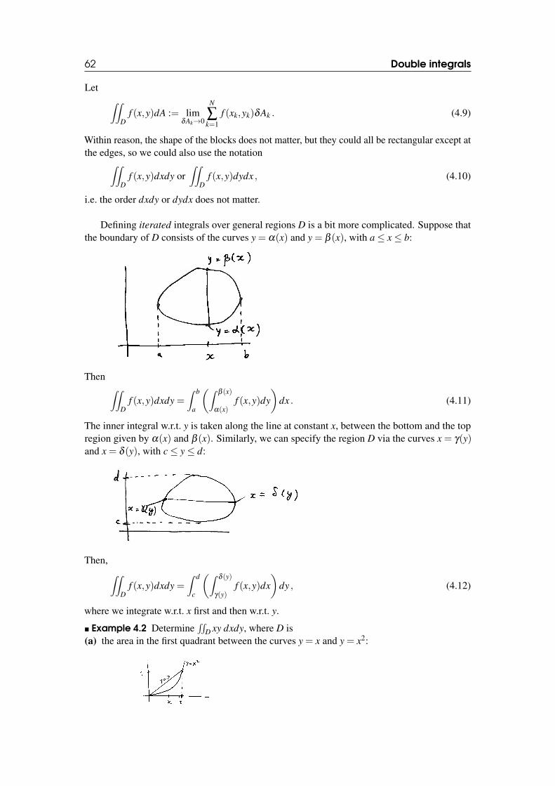
62 Double integrals
Let ∫∫D
f (x,y)dA := limδAk→0
N
∑k=1
f (xk,yk)δAk . (4.9)
Within reason, the shape of the blocks does not matter, but they could all be rectangular except atthe edges, so we could also use the notation∫∫
Df (x,y)dxdy or
∫∫D
f (x,y)dydx , (4.10)
i.e. the order dxdy or dydx does not matter.
Defining iterated integrals over general regions D is a bit more complicated. Suppose thatthe boundary of D consists of the curves y = α(x) and y = β (x), with a≤ x≤ b:
Then ∫∫D
f (x,y)dxdy =∫ b
a
(∫β (x)
α(x)f (x,y)dy
)dx . (4.11)
The inner integral w.r.t. y is taken along the line at constant x, between the bottom and the topregion given by α(x) and β (x). Similarly, we can specify the region D via the curves x = γ(y)and x = δ (y), with c≤ y≤ d:
Then, ∫∫D
f (x,y)dxdy =∫ d
c
(∫δ (y)
γ(y)f (x,y)dx
)dy , (4.12)
where we integrate w.r.t. x first and then w.r.t. y.
� Example 4.2 Determine∫∫
D xy dxdy, where D is(a) the area in the first quadrant between the curves y = x and y = x2:
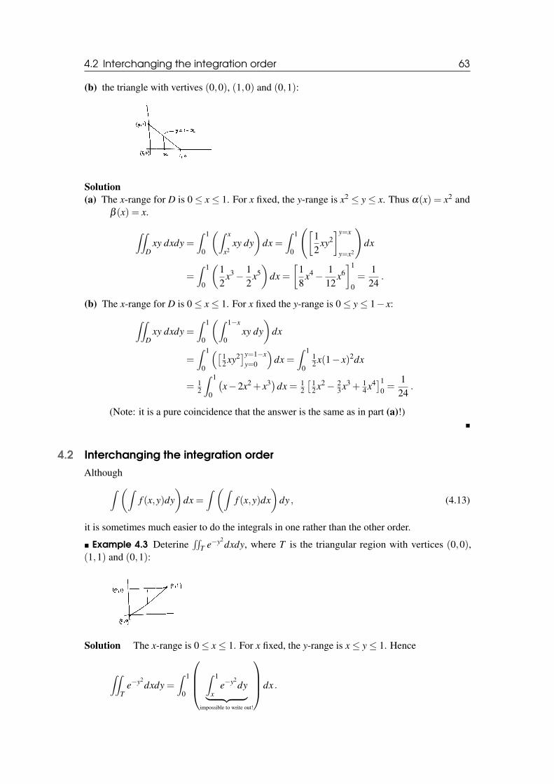
4.2 Interchanging the integration order 63
(b) the triangle with vertives (0,0), (1,0) and (0,1):
Solution(a) The x-range for D is 0≤ x≤ 1. For x fixed, the y-range is x2 ≤ y≤ x. Thus α(x) = x2 and
β (x) = x.
∫∫D
xy dxdy =∫ 1
0
(∫ x
x2xy dy
)dx =
∫ 1
0
([12
xy2]y=x
y=x2
)dx
=∫ 1
0
(12
x3− 12
x5)
dx =[
18
x4− 112
x6]1
0=
124
.
(b) The x-range for D is 0≤ x≤ 1. For x fixed the y-range is 0≤ y≤ 1− x:∫∫D
xy dxdy =∫ 1
0
(∫ 1−x
0xy dy
)dx
=∫ 1
0
([12 xy2]y=1−x
y=0
)dx =
∫ 1
0
12 x(1− x)2dx
= 12
∫ 1
0
(x−2x2 + x3)dx = 1
2
[12 x2− 2
3 x3 + 14 x4]1
0 =1
24.
(Note: it is a pure coincidence that the answer is the same as in part (a)!)�
4.2 Interchanging the integration orderAlthough∫ (∫
f (x,y)dy)
dx =∫ (∫
f (x,y)dx)
dy , (4.13)
it is sometimes much easier to do the integrals in one rather than the other order.
� Example 4.3 Deterine∫∫
T e−y2dxdy, where T is the triangular region with vertices (0,0),
(1,1) and (0,1):
Solution The x-range is 0≤ x≤ 1. For x fixed, the y-range is x≤ y≤ 1. Hence
∫∫T
e−y2dxdy =
∫ 1
0
∫ 1
xe−y2
dy︸ ︷︷ ︸impossible to write out!
dx .
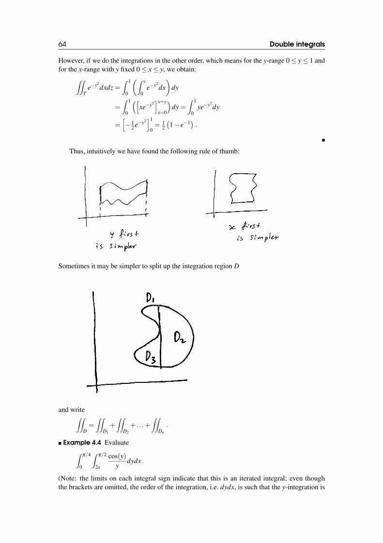
64 Double integrals
However, if we do the integrations in the other order, which means for the y-range 0≤ y≤ 1 andfor the x-range with y fixed 0≤ x≤ y, we obtain:∫∫
Te−y2
dxdz =∫ 1
0
(∫ y
0e−y2
dx)
dy
=∫ 1
0
([xe−y2
]x=y
x=0
)dy =
∫ 1
0ye−y2
dy
=[−1
2 e−y2]1
0= 1
2
(1− e−1) .
�
Thus, intuitively we have found the following rule of thumb:
Sometimes it may be simpler to split up the integration region D
and write∫∫D=∫∫
D1
+∫∫
D2
+ . . .+∫∫
Dn
.
� Example 4.4 Evaluate∫π/4
0
∫π/2
2x
cos(y)y
dydx .
(Note: the limits on each integral sign indicate that this is an iterated integral; even thoughthe brackets are omitted, the order of the integration, i.e. dydx, is such that the y-integration is
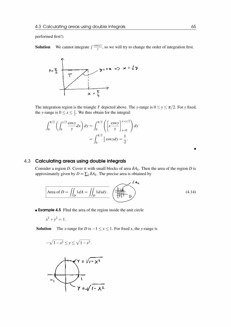
4.3 Calculating areas using double integrals 65
performed first!)
Solution We cannot integrate∫ cos(y)
y , so we will try to change the order of integration first.
The integration region is the triangle T depicted above. The y-range is 0≤ y≤ π/2. For y fixed,the y-range is 0≤ x≤ y
2 . We thus obtain for the integral:
∫π/2
0
(∫ y/2
0
cosyy
dx)
dy =∫
π/2
0
([x
cosyy
]x=y/2
x=0
)dy
=∫
π/2
0
12 cosydy =
12.
�
4.3 Calculating areas using double integralsConsider a region D. Cover it with small blocks of area δAk. Then the area of the region D isapproximately given by D≈ ∑k δAk. The precise area is obtained by
Area of D =∫∫
D1dA =
∫∫D
1dxdy . (4.14)
� Example 4.5 FInd the area of the region inside the unit circle
x2 + y2 = 1 .
Solution The x-range for D is −1≤ x≤ 1. For fixed x, the y-range is
−√
1− x2 ≤ y≤√
1− x2 .
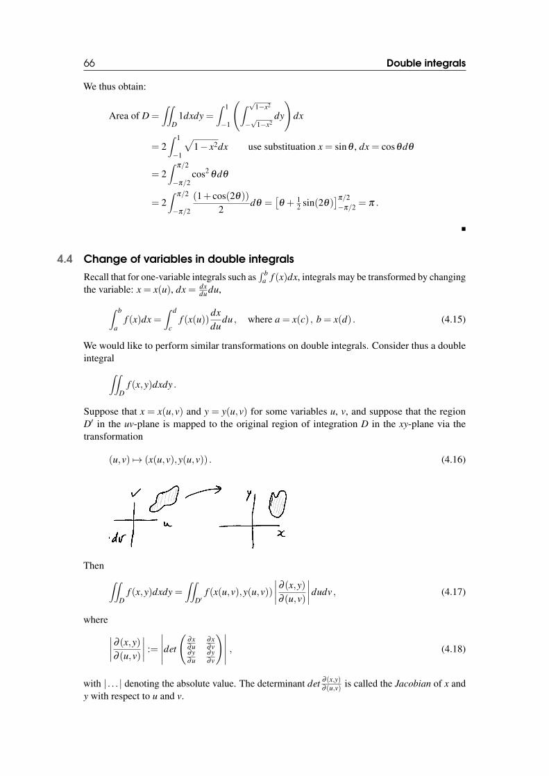
66 Double integrals
We thus obtain:
Area of D =∫∫
D1dxdy =
∫ 1
−1
(∫ √1−x2
−√
1−x2dy
)dx
= 2∫ 1
−1
√1− x2dx use substituation x = sinθ , dx = cosθdθ
= 2∫
π/2
−π/2cos2
θdθ
= 2∫
π/2
−π/2
(1+ cos(2θ))
2dθ =
[θ + 1
2 sin(2θ)]π/2−π/2 = π .
�
4.4 Change of variables in double integrals
Recall that for one-variable integrals such as∫ b
a f (x)dx, integrals may be transformed by changingthe variable: x = x(u), dx = dx
du du,
∫ b
af (x)dx =
∫ d
cf (x(u))
dxdu
du , where a = x(c) , b = x(d) . (4.15)
We would like to perform similar transformations on double integrals. Consider thus a doubleintegral∫∫
Df (x,y)dxdy .
Suppose that x = x(u,v) and y = y(u,v) for some variables u, v, and suppose that the regionD′ in the uv-plane is mapped to the original region of integration D in the xy-plane via thetransformation
(u,v) 7→ (x(u,v),y(u,v)) . (4.16)
Then ∫∫D
f (x,y)dxdy =∫∫
D′f (x(u,v),y(u,v))
∣∣∣∣∂ (x,y)∂ (u,v)
∣∣∣∣dudv , (4.17)
where∣∣∣∣∂ (x,y)∂ (u,v)
∣∣∣∣ :=
∣∣∣∣∣det
(∂x∂u
∂x∂v
∂y∂u
∂y∂v
)∣∣∣∣∣ , (4.18)
with | . . . | denoting the absolute value. The determinant det ∂ (x,y)∂ (u,v) is called the Jacobian of x and
y with respect to u and v.
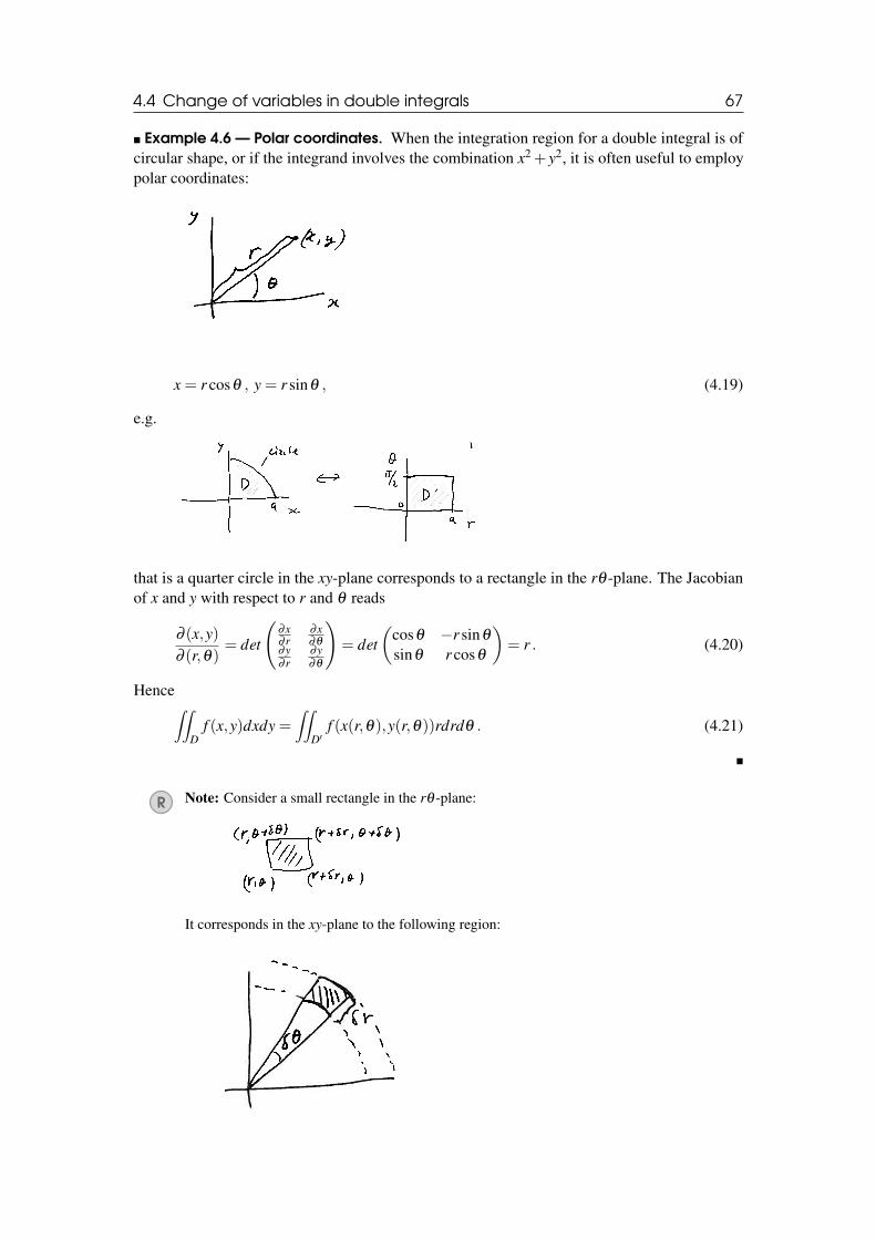
4.4 Change of variables in double integrals 67
� Example 4.6 — Polar coordinates. When the integration region for a double integral is ofcircular shape, or if the integrand involves the combination x2 + y2, it is often useful to employpolar coordinates:
x = r cosθ , y = r sinθ , (4.19)
e.g.
that is a quarter circle in the xy-plane corresponds to a rectangle in the rθ -plane. The Jacobianof x and y with respect to r and θ reads
∂ (x,y)∂ (r,θ)
= det
(∂x∂ r
∂x∂θ
∂y∂ r
∂y∂θ
)= det
(cosθ −r sinθ
sinθ r cosθ
)= r . (4.20)
Hence∫∫D
f (x,y)dxdy =∫∫
D′f (x(r,θ),y(r,θ))rdrdθ . (4.21)
�
R Note: Consider a small rectangle in the rθ -plane:
It corresponds in the xy-plane to the following region:
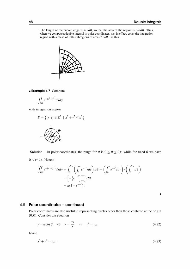
68 Double integrals
The length of the curved edge is ≈ rδθ , so that the area of the region is rδ rδθ . Thus,when we compute a duoble integral in polar coordinates, we, in effect, cover the integrationregion with a mesh of little subregions of area rδ rδθ like this:
� Example 4.7 Compute∫∫D
e−(x2+y2)dxdy
with integration region
D ={(x,y) ∈ R2 | x2 + y2 ≤ a2}
Solution In polar coordinates, the range for θ is 0 ≤ θ ≤ 2π , while for fixed θ we have
0≤ r ≤ a. Hence:∫∫D
e−(x2+y2)dxdy =
∫ 2π
0
(∫ a
0e−r2
rdr)
dθ =
(∫ a
0e−r2
rdr)·(∫ 2π
0dθ
)=[−1
2 e−r2]r=a
r=0·2π
= π(1− e−a2) .
�
4.5 Polar coordinates – continued
Polar coordinates are also useful in representing circles other than those centered at the origin(0,0). Consider the equation
r = acosθ ⇔ r =axr
⇔ r2 = ax , (4.22)
hence
x2 + y2 = ax . (4.23)
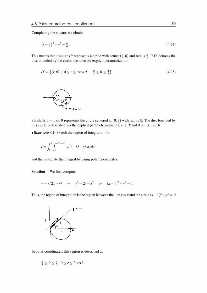
4.5 Polar coordinates – continued 69
Completing the square, we obtain
(x− a
2
)2+ y2 = a
4 . (4.24)
This means that r = acosθ represents a circle with center (a2 ,0) and radius a
2 . If D′ denotes thedisc bounded by the circle, we have the explicit parametrization
D′ ={(r,θ) | 0≤ r ≤ acosθ , −π
2 ≤ θ ≤ π
2
}. (4.25)
Similarly, r = asinθ represents the circle centered at (0, a2) with radius a
2 . The disc bounded bythis circle is described via the explicit parametrization 0≤ θ ≤ π and 0≤ r ≤ asinθ .
� Example 4.8 Sketch the region of integration for
I =∫ 1
0
∫ √2x−x2
x
√4− x2− y2 dydx
and then evaluate the integral by using polar coordinates.
Solution We first compute
y =√
2x− x2 ⇒ y2 = 2x− x2 ⇔ (x−1)2 + y2 = 1 .
Thus, the region of integration is the region between the line y= x and the circle (x−1)2+y2 = 1:
In polar coordinates, this region is described as
π
4 ≤ θ ≤ π
2 , 0≤ r ≤ 2cosθ .
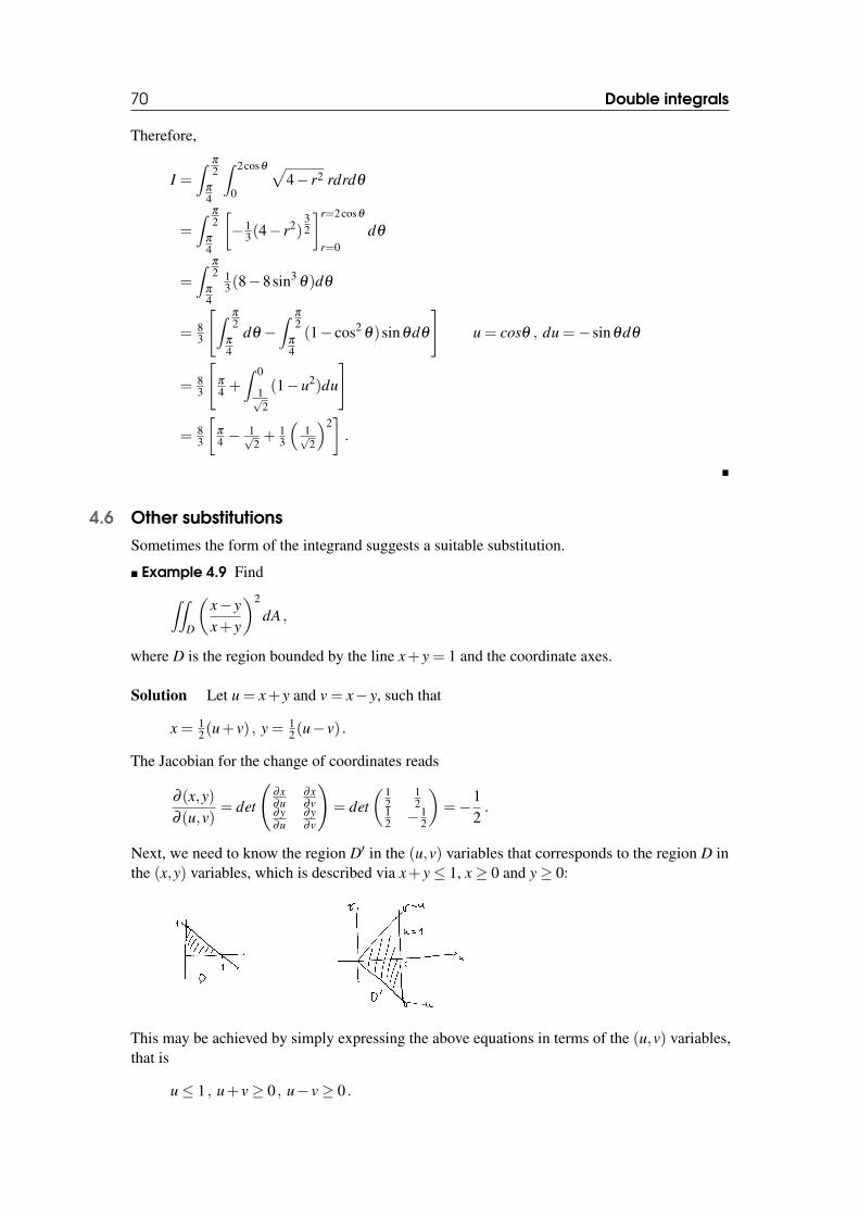
70 Double integrals
Therefore,
I =∫ π
2π
4
∫ 2cosθ
0
√4− r2 rdrdθ
=∫ π
2π
4
[−1
3(4− r2)32
]r=2cosθ
r=0dθ
=∫ π
2π
4
13(8−8sin3
θ)dθ
= 83
[∫ π
2π
4
dθ −∫ π
2π
4
(1− cos2θ)sinθdθ
]u = cosθ , du =−sinθdθ
= 83
[π
4 +∫ 0
1√2
(1−u2)du
]
= 83
[π
4 −1√2+ 1
3
(1√2
)2].
�
4.6 Other substitutionsSometimes the form of the integrand suggests a suitable substitution.
� Example 4.9 Find∫∫D
(x− yx+ y
)2
dA ,
where D is the region bounded by the line x+ y = 1 and the coordinate axes.
Solution Let u = x+ y and v = x− y, such that
x = 12(u+ v) , y = 1
2(u− v) .
The Jacobian for the change of coordinates reads
∂ (x,y)∂ (u,v)
= det
(∂x∂u
∂x∂v
∂y∂u
∂y∂v
)= det
(12
12
12 −1
2
)=−1
2.
Next, we need to know the region D′ in the (u,v) variables that corresponds to the region D inthe (x,y) variables, which is described via x+ y≤ 1, x≥ 0 and y≥ 0:
This may be achieved by simply expressing the above equations in terms of the (u,v) variables,that is
u≤ 1 , u+ v≥ 0 , u− v≥ 0 .
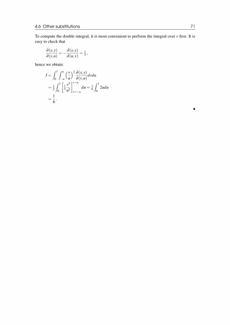
4.6 Other substitutions 71
To compute the double integral, it is most convenient to perform the integral over v first. It iseasy to check that
∂ (x,y)∂ (v,u)
=−∂ (x,y)∂ (u,v)
= 12 ,
hence we obtain:
I =∫ 1
0
∫ u
−u
( vu
)2 ∂ (x,y)∂ (v,u)
dvdu
= 12
∫ 1
0
[13
v3
u2
]v=u
v=−udu = 1
6
∫ 1
02udu
=16.
�

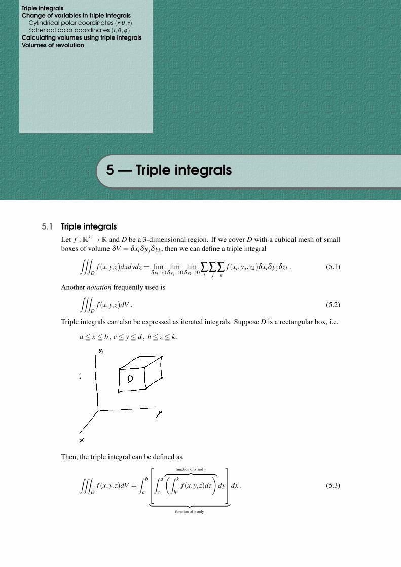
Triple integralsChange of variables in triple integrals
Cylindrical polar coordinates (r,θ ,z)Spherical polar coordinates (r,θ ,φ)
Calculating volumes using triple integralsVolumes of revolution
5 — Triple integrals
5.1 Triple integralsLet f : R3→ R and D be a 3-dimensional region. If we cover D with a cubical mesh of smallboxes of volume δV = δxiδy jδyk, then we can define a triple integral∫∫∫
Df (x,y,z)dxdydz = lim
δxi→0lim
δy j→0lim
δyk→0∑
i∑
j∑k
f (xi,y j,zk)δxiδy jδ zk . (5.1)
Another notation frequently used is∫∫∫D
f (x,y,z)dV . (5.2)
Triple integrals can also be expressed as iterated integrals. Suppose D is a rectangular box, i.e.
a≤ x≤ b , c≤ y≤ d , h≤ z≤ k .
Then, the triple integral can be defined as
∫∫∫D
f (x,y,z)dV =∫ b
a
∫ d
c
function of x and y︷ ︸︸ ︷(∫ k
hf (x,y,z)dz
)dy
︸ ︷︷ ︸
function of x only
dx . (5.3)
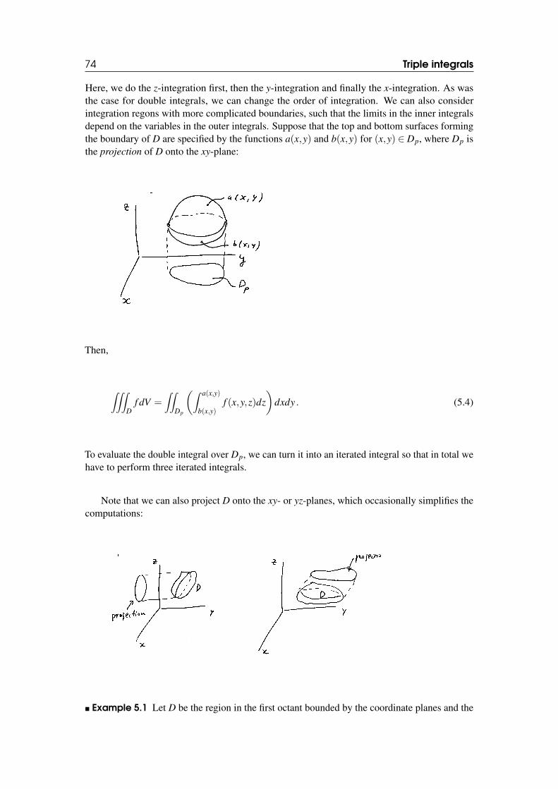
74 Triple integrals
Here, we do the z-integration first, then the y-integration and finally the x-integration. As wasthe case for double integrals, we can change the order of integration. We can also considerintegration regons with more complicated boundaries, such that the limits in the inner integralsdepend on the variables in the outer integrals. Suppose that the top and bottom surfaces formingthe boundary of D are specified by the functions a(x,y) and b(x,y) for (x,y) ∈ Dp, where Dp isthe projection of D onto the xy-plane:
Then,
∫∫∫D
f dV =∫∫
Dp
(∫ a(x,y)
b(x,y)f (x,y,z)dz
)dxdy . (5.4)
To evaluate the double integral over Dp, we can turn it into an iterated integral so that in total wehave to perform three iterated integrals.
Note that we can also project D onto the xy- or yz-planes, which occasionally simplifies thecomputations:
� Example 5.1 Let D be the region in the first octant bounded by the coordinate planes and the
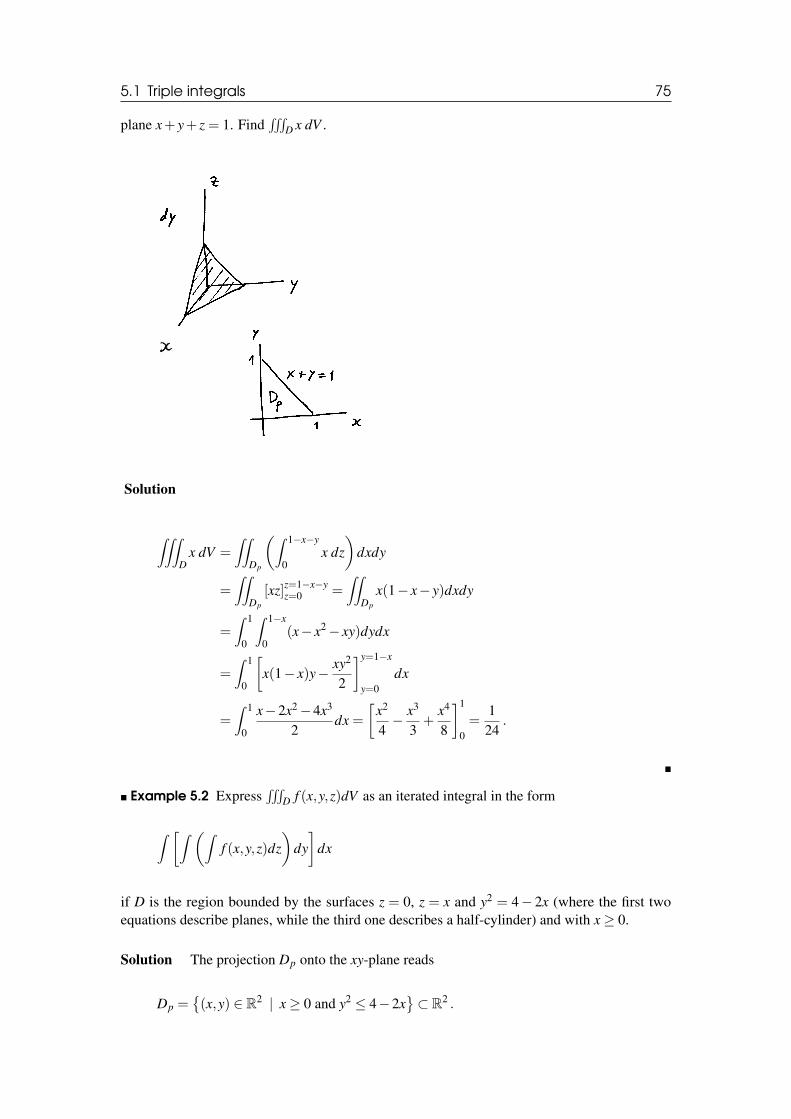
5.1 Triple integrals 75
plane x+ y+ z = 1. Find∫∫∫
D x dV .
Solution
∫∫∫D
x dV =∫∫
Dp
(∫ 1−x−y
0x dz
)dxdy
=∫∫
Dp
[xz]z=1−x−yz=0 =
∫∫Dp
x(1− x− y)dxdy
=∫ 1
0
∫ 1−x
0(x− x2− xy)dydx
=∫ 1
0
[x(1− x)y− xy2
2
]y=1−x
y=0dx
=∫ 1
0
x−2x2−4x3
2dx =
[x2
4− x3
3+
x4
8
]1
0=
124
.
�
� Example 5.2 Express∫∫∫
D f (x,y,z)dV as an iterated integral in the form
∫ [∫ (∫f (x,y,z)dz
)dy]
dx
if D is the region bounded by the surfaces z = 0, z = x and y2 = 4− 2x (where the first twoequations describe planes, while the third one describes a half-cylinder) and with x≥ 0.
Solution The projection Dp onto the xy-plane reads
Dp ={(x,y) ∈ R2 | x≥ 0 and y2 ≤ 4−2x
}⊂ R2 .
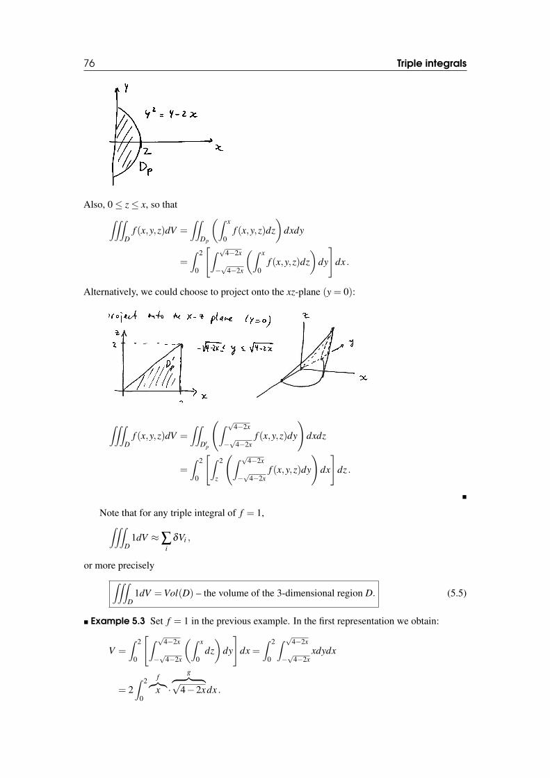
76 Triple integrals
Also, 0≤ z≤ x, so that∫∫∫D
f (x,y,z)dV =∫∫
Dp
(∫ x
0f (x,y,z)dz
)dxdy
=∫ 2
0
[∫ √4−2x
−√
4−2x
(∫ x
0f (x,y,z)dz
)dy
]dx .
Alternatively, we could choose to project onto the xz-plane (y = 0):
∫∫∫D
f (x,y,z)dV =∫∫
D′p
(∫ √4−2x
−√
4−2xf (x,y,z)dy
)dxdz
=∫ 2
0
[∫ 2
z
(∫ √4−2x
−√
4−2xf (x,y,z)dy
)dx
]dz .
�
Note that for any triple integral of f = 1,∫∫∫D
1dV ≈∑i
δVi ,
or more precisely∫∫∫D
1dV =Vol(D) – the volume of the 3-dimensional region D. (5.5)
� Example 5.3 Set f = 1 in the previous example. In the first representation we obtain:
V =∫ 2
0
[∫ √4−2x
−√
4−2x
(∫ x
0dz)
dy
]dx =
∫ 2
0
∫ √4−2x
−√
4−2xxdydx
= 2∫ 2
0
f︷︸︸︷x ·
g︷ ︸︸ ︷√4−2xdx .
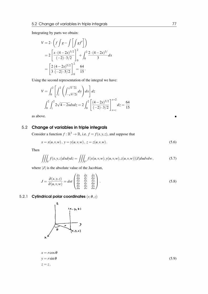
5.2 Change of variables in triple integrals 77
Integrating by parts we obtain:
V = 2 ·(
f∫
g−∫ [∫
g f ′])
= 2
[x · (4−2x)3/2
(−2) ·3/2
]2
0
+∫ 2
0
2 · (4−2x)3/
3dx
=
[23(4−2x)5/2
(−2) ·5/2
]2
0
=6415
.
Using the second representation of the integral we have:
V =∫ 2
0
[∫ 2
z
(∫ √4−2x
−√
4−2xdy
)dx
]dz
∫ 2
0
∫ 2
z2√
4−2xdxdz = 2∫ 2
0
[(4−2x)3/2
(−2) ·3/2
]x=2
x=z
dz =6415
as above. �
5.2 Change of variables in triple integralsConsider a function f : R3→ R, i.e. f = f (x,y,z), and suppose that
x = x(u,v,w) , y = y(u,v,w) , z = z(u,v,w) . (5.6)
Then ∫∫∫V
f (x,y,z)dxdydz =∫∫∫
V ′f (x(u,v,w),y(u,v,w),z(u,v,w))|J|dudvdw , (5.7)
where |J| is the absolute value of the Jacobian,
J =∂ (x,y,z)∂ (u,v,w)
= det
∂x∂u
∂x∂v
∂x∂w
∂y∂u
∂y∂v
∂y∂w
∂ z∂u
∂ z∂v
∂ z∂w
. (5.8)
5.2.1 Cylindrical polar coordinates (r,θ ,z)
x = r cosθ
y = r sinθ
z = z ,
(5.9)
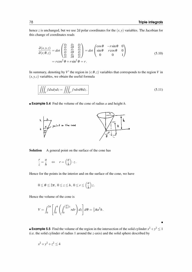
78 Triple integrals
hence z is unchanged, but we use 2d polar coordinates for the (x,y) variables. The Jacobian forthis change of coordinates reads
∂ (x,y,z)∂ (r,θ ,z)
= det
∂x∂ r
∂x∂θ
∂x∂ z
∂y∂ r
∂y∂θ
∂y∂ z
∂ z∂ r
∂ z∂θ
∂ z∂ z
= det
cosθ −r sinθ 0sinθ r cosθ 0
0 0 1
= r cos2
θ + r sin2θ = r .
(5.10)
In summary, denoting by V ′ the region in (r,θ ,z) variables that corresponds to the region V in(x,y,z) variables, we obtain the useful formula
∫∫∫V
f dxdydz =∫∫∫
V ′f rdrdθdz . (5.11)
� Example 5.4 Fnd the volume of the cone of radius a and height h.
Solution A general point on the surface of the cone has
rz=
ah⇔ r =
(ah
)· z .
Hence for the points in the interior and on the surface of the cone, we have
0≤ θ ≤ 2π , 0≤ z≤ h , 0≤ r ≤(a
h
)z .
Hence the volume of the cone is
V =∫ 2π
0
[∫ h
0
(∫ (ah)z
0rdr
)dz
]dθ = 1
3 πa2h .
�
� Example 5.5 Find the volume of the region in the intersection of the solid cylinder x2+y2 ≤ 1(i.e. the solid cylinder of radius 1 around the z-axis) and the solid sphere described by
x2 + y2 + z2 ≤ 4
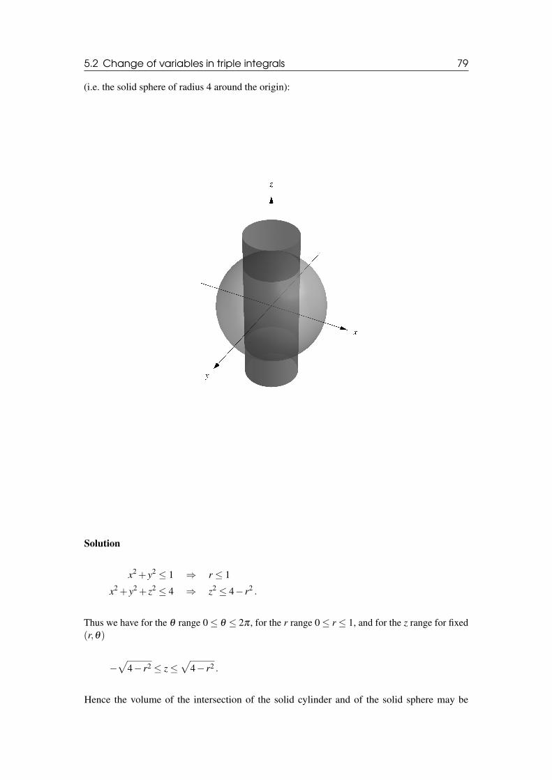
5.2 Change of variables in triple integrals 79
(i.e. the solid sphere of radius 4 around the origin):
Solution
x2 + y2 ≤ 1 ⇒ r ≤ 1
x2 + y2 + z2 ≤ 4 ⇒ z2 ≤ 4− r2 .
Thus we have for the θ range 0≤ θ ≤ 2π , for the r range 0≤ r ≤ 1, and for the z range for fixed(r,θ)
−√
4− r2 ≤ z≤√
4− r2 .
Hence the volume of the intersection of the solid cylinder and of the solid sphere may be
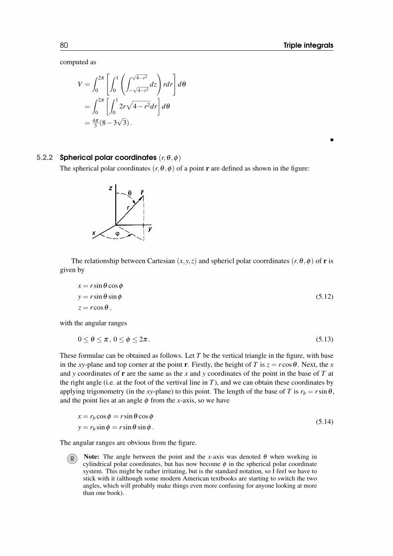
80 Triple integrals
computed as
V =∫ 2π
0
[∫ 1
0
(∫ √4−r2
−√
4−r2dz
)rdr
]dθ
=∫ 2π
0
[∫ 1
02r√
4− r2dr]
dθ
= 4π
3 (8−3√
3) .
�
5.2.2 Spherical polar coordinates (r,θ ,φ)The spherical polar coordinates (r,θ ,φ) of a point r are defined as shown in the figure:
The relationship between Cartesian (x,y,z) and sphericl polar coorrdinates (r,θ ,φ) of r isgiven by
x = r sinθ cosφ
y = r sinθ sinφ
z = r cosθ ,
(5.12)
with the angular ranges
0≤ θ ≤ π , 0≤ φ ≤ 2π . (5.13)
These formulae can be obtained as follows. Let T be the vertical triangle in the figure, with basein the xy-plane and top corner at the point r. Firstly, the height of T is z = r cosθ . Next, the xand y coordinates of r are the same as the x and y coordinates of the point in the base of T atthe right angle (i.e. at the foot of the vertival line in T ), and we can obtain these coordinates byapplying trigonometry (in the xy-plane) to this point. The length of the base of T is rb = r sinθ ,and the point lies at an angle φ from the x-axis, so we have
x = rb cosφ = r sinθ cosφ
y = rb sinφ = r sinθ sinφ .(5.14)
The angular ranges are obvious from the figure.
R Note: The angle between the point and the x-axis was denoted θ when working incylindrical polar coordinates, but has now become φ in the spherical polar coordinatesystem. This might be rather irritating, but is the standard notation, so I feel we have tostick with it (although some modern American textbooks are starting to switch the twoangles, which will probably make things even more confusing for anyone looking at morethan one book).
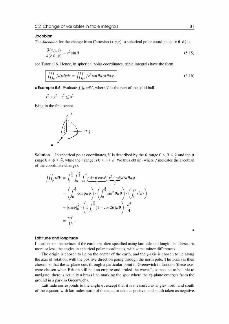
5.2 Change of variables in triple integrals 81
JacobianThe Jacobian for the change from Cartesian (x,y,z) to spherical polar coordinates (r,θ ,φ) is
∂ (x,y,z)∂ (r,θ ,φ)
= r2 sinθ (5.15)
see Tutorial 6. Hence, in spherical polar coordinates, triple integrals have the form∫∫∫V
f dxdydz =∫∫∫
V ′f r2 sinθdrdθdφ . (5.16)
� Example 5.6 Evaluate∫∫∫
V xdV , where V is the part of the solid ball
x2 + y2 + z2 ≤ a2
lying in the first octant.
Solution In spherical polar coordinates, V is described by the θ range 0≤ θ ≤ π
2 and the φ
range 0≤ φ ≤ π
2 , while the r range is 0≤ r ≤ a. We thus obtain (where J indicates the Jacobianof the coordinate change):
∫∫∫V
xdV =∫ π
2
0
∫ π
2
0
∫ a
0r sinθ cosφ︸ ︷︷ ︸
x
·r2 sinθ︸ ︷︷ ︸J
drdθdφ
=
(∫ π
2
0cosφdφ
)·
(∫ π
2
0sin2
θdθ
)·(∫ a
0r2dr
)
= [sinφ ]π
20 ·
(12
∫ π
2
0(1− cos2θ)dθ
)· a
4
4
=πa4
16.
�
Lattitude and longitudeLocations on the surface of the earth are often specified using lattitude and longitude. These are,more or less, the angles in spherical polar coordinates, with some minor differences.
The origin is chosen to lie on the center of the earth, and the z-axis is chosen to lie alongthe axis of rotation, with the positive direction going through the north pole. The x-axis is thenchosen so that the xz-plane cuts through a particular point in Greenwich in London (these axeswere chosen when Britain still had an empire and “ruled the waves”, so needed to be able tonavigate; there is actually a brass line marking the spot where the xz-plane emerges from theground in a park in Greenwich).
Lattitude corresponds to the angle θ , except that it is measured as angles north and southof the equator, with lattitudes north of the equator takn as positve, and south taken as negative.
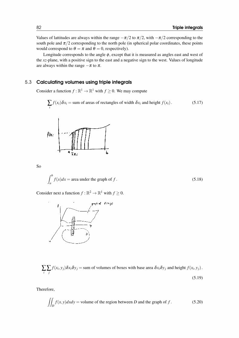
82 Triple integrals
Values of lattitudes are always within the range −π/2 to π/2, with −π/2 corresponding to thesouth pole and π/2 corresponding to the north pole (in spherical polar coordinates, these pointswould correspond to θ = π and θ = 0, respectively).
Longitude corresponds to the angle φ , except that it is measured as angles east and west ofthe xz-plane, with a positive sign to the east and a negative sign to the west. Values of longitudeare always within the range −π to π .
5.3 Calculating volumes using triple integrals
Consider a function f : R1→ R1 with f ≥ 0. We may compute
∑i
f (xi)δxi = sum of areas of rectangles of width δxi and height f (xi) . (5.17)
So
∫ b
af (x)dx = area under the graph of f . (5.18)
Consider next a function f : R2→ R1 with f ≥ 0.
∑i
∑j
f (xi,y j)δxiδy j = sum of volumes of boxes with base area δxiδy j and height f (xi,y j) .
(5.19)
Therefore,∫∫D
f (x,y)dxdy = volume of the region between D and the graph of f . (5.20)
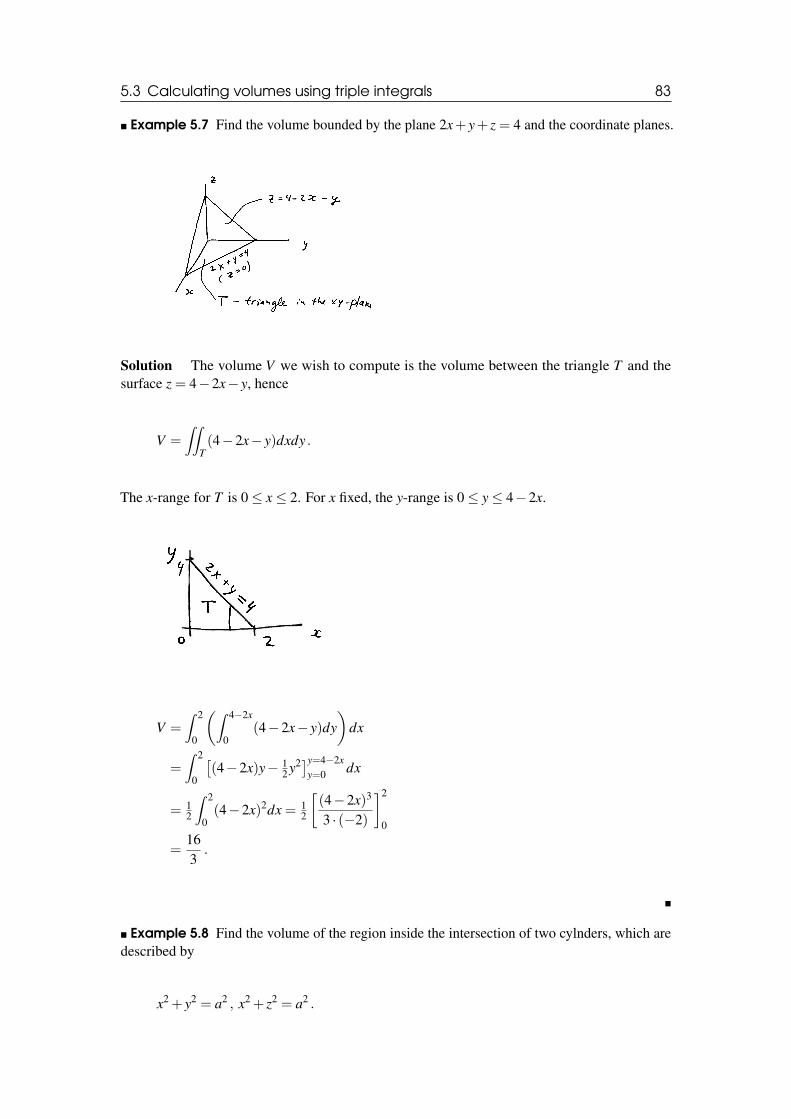
5.3 Calculating volumes using triple integrals 83
� Example 5.7 Find the volume bounded by the plane 2x+ y+ z = 4 and the coordinate planes.
Solution The volume V we wish to compute is the volume between the triangle T and thesurface z = 4−2x− y, hence
V =∫∫
T(4−2x− y)dxdy .
The x-range for T is 0≤ x≤ 2. For x fixed, the y-range is 0≤ y≤ 4−2x.
V =∫ 2
0
(∫ 4−2x
0(4−2x− y)dy
)dx
=∫ 2
0
[(4−2x)y− 1
2 y2]y=4−2xy=0 dx
= 12
∫ 2
0(4−2x)2dx = 1
2
[(4−2x)3
3 · (−2)
]2
0
=163.
�
� Example 5.8 Find the volume of the region inside the intersection of two cylnders, which aredescribed by
x2 + y2 = a2 , x2 + z2 = a2 .
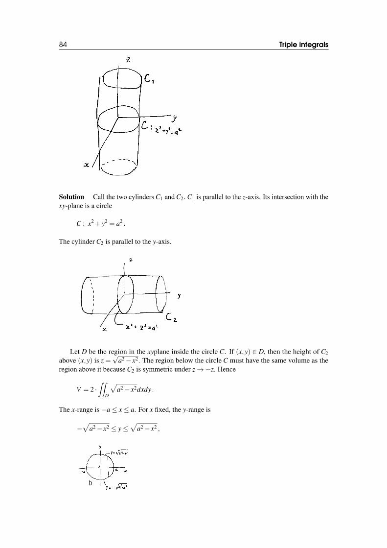
84 Triple integrals
Solution Call the two cylinders C1 and C2. C1 is parallel to the z-axis. Its intersection with thexy-plane is a circle
C : x2 + y2 = a2 .
The cylinder C2 is parallel to the y-axis.
Let D be the region in the xyplane inside the circle C. If (x,y) ∈ D, then the height of C2above (x,y) is z =
√a2− x2. The region below the circle C must have the same volume as the
region above it because C2 is symmetric under z→−z. Hence
V = 2 ·∫∫
D
√a2− x2dxdy .
The x-range is −a≤ x≤ a. For x fixed, the y-range is
−√
a2− x2 ≤ y≤√
a2− x2 ,
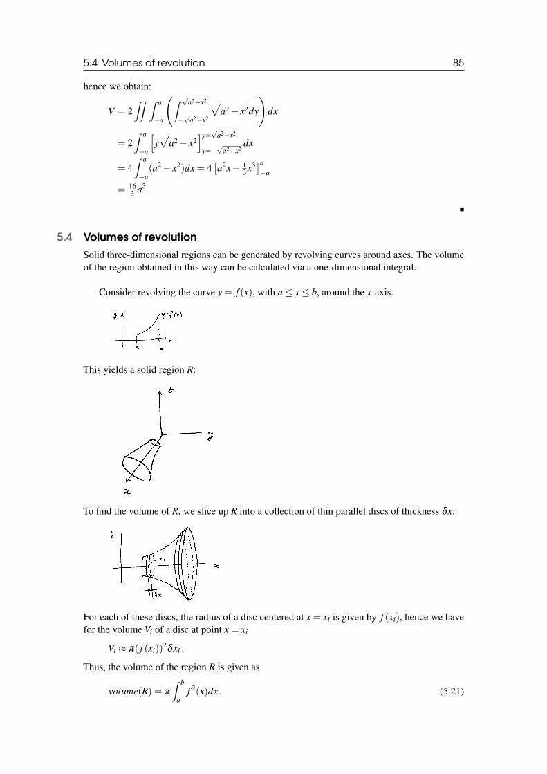
5.4 Volumes of revolution 85
hence we obtain:
V = 2∫∫ ∫ a
−a
(∫ √a2−x2
−√
a2−x2
√a2− x2dy
)dx
= 2∫ a
−a
[y√
a2− x2]y=√
a2−x2
y=−√
a2−x2dx
= 4∫ a
−a(a2− x2)dx = 4
[a2x− 1
3 x3]a−a
= 163 a3 .
�
5.4 Volumes of revolutionSolid three-dimensional regions can be generated by revolving curves around axes. The volumeof the region obtained in this way can be calculated via a one-dimensional integral.
Consider revolving the curve y = f (x), with a≤ x≤ b, around the x-axis.
This yields a solid region R:
To find the volume of R, we slice up R into a collection of thin parallel discs of thickness δx:
For each of these discs, the radius of a disc centered at x = xi is given by f (xi), hence we havefor the volume Vi of a disc at point x = xi
Vi ≈ π( f (xi))2δxi .
Thus, the volume of the region R is given as
volume(R) = π
∫ b
af 2(x)dx . (5.21)
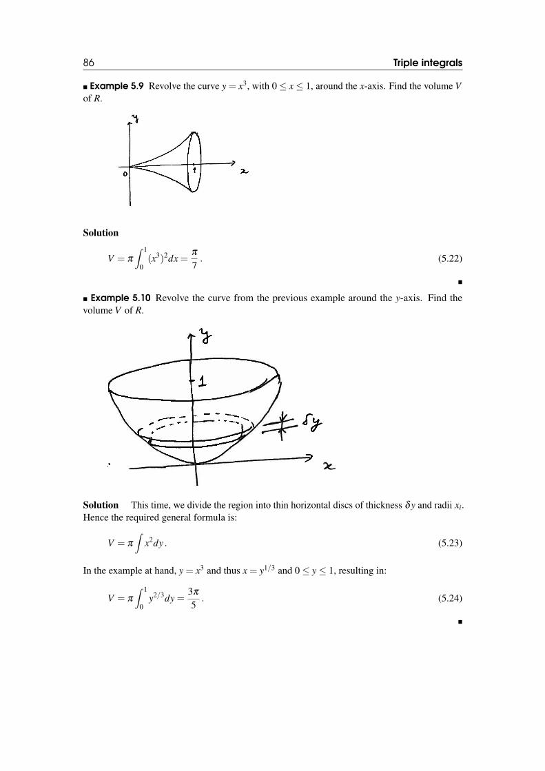
86 Triple integrals
� Example 5.9 Revolve the curve y = x3, with 0≤ x≤ 1, around the x-axis. Find the volume Vof R.
Solution
V = π
∫ 1
0(x3)2dx =
π
7. (5.22)
�
� Example 5.10 Revolve the curve from the previous example around the y-axis. Find thevolume V of R.
Solution This time, we divide the region into thin horizontal discs of thickness δy and radii xi.Hence the required general formula is:
V = π
∫x2dy . (5.23)
In the example at hand, y = x3 and thus x = y1/3 and 0≤ y≤ 1, resulting in:
V = π
∫ 1
0y2/3dy =
3π
5. (5.24)
�
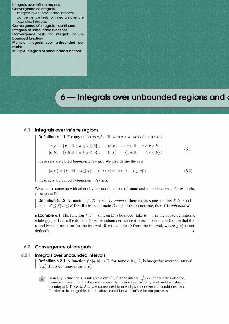
Integrals over infinite regionsConvergence of integrals
Integrals over unbounded intervalsConvergence tests for integrals over un-bounded intervals
Convergence of integrals – continuedIntegrals of unbounded functionsConvergence tests for integrals of un-bounded functionsMultiple integrals over unbounded do-mainsMultiple integrals of unbounded functions
6 — Integrals over unbounded regions and of unbounded functions
6.1 Integrals over infinite regionsDefinition 6.1.1 For any numbers a,b ∈ R, with a < b, we define the sets
[a,b] = {x ∈ R | a≤ x≤ b} , (a,b) = {x ∈ R | a < x < b} ,[a,b) = {x ∈ R | a≤ x < b} , (a,b] = {x ∈ R | a < x≤ b} ;
(6.1)
these sets are called bounded intervals. We also define the sets
[a,∞) = {x ∈ R | a≤ x} , (−∞,a] = {x ∈ R | x≤ a} ; (6.2)
these sets are called unbounded intervals.
We can also come up with other obvious combinations of round and square brackets. For example,(−∞,∞) = R.
Definition 6.1.2 A function f : D→ R is bounded if there exists some number K ≥ 0 suchthat −K ≤ f (x)≤ K for all x in the domain D of f ; if this is not true, then f is unbounded.
� Example 6.1 The function f (x) = sinx on R is bounded (take K = 1 in the above definition),while g(x) = 1/x in the domain (0,∞) is unbounded, since it blows up near x = 0 (note that theround bracket notation for the interval (0,∞) excludes 0 from the interval, where g(x) is notdefined). �
6.2 Convergence of integrals
6.2.1 Integrals over unbounded intervalsDefinition 6.2.1 A function f : [a,b]→ R, for some a,b ∈ R, is integrable over the interval[a,b] if it is continuous on [a,b].
R Basically, a function f is integrable over [a,b] if the integral∫ b
a f (x)dx has a well-defined,theoretical meaning (this does not necessarily mean we can actually work out the value ofthe integral). The Real Analysis course next term will give more general conditions for afunction to be integrable, but the above condition will suffice for our purposes.
88 Integrals over unbounded regions and of unbounded functions
We now want to define the idea of an integral over an infinite interval, say [a,∞), for some a ∈R.Clearly, to integrate a function f : [a,∞)→ R over [a,∞), we will need it to be integrable overany finite interval [a,b].
Definition 6.2.2 Suppose that f : [a,∞)→ R is integrable over [a, t] for any t ≥ a. Then theinfinite integral
∫∞
a f (x)dx is defined as∫∞
af (x)dx = lim
t→∞
∫ t
af (x)dx . (6.3)
If this integral exists and is finite, we say that the integral converges. If the limit does notexist, or if the integral gives an infinite value, then we say that the integral diverges (and thusdoes not have a value).
For a function f : (−∞,a]→R, we define convergence and divegence of∫ a−∞
f (x)dx analogously.We can also define convergence and divergence of
∫∞
−∞f (x)dx by analyzing the convergence and
divergence of the integrals∫ 0−∞
f (x)dx and∫
∞
0 f (x)dx separately.
� Example 6.2 Show that the integral∫
∞
0 1dx (i.e. the integral over the constant function 1)diverges.
Solution∫∞
01dx = lim
t→∞
∫ t
0dx = lim
t→∞t = ∞ ,
hence the integral diverges. �
� Example 6.3 Show that the integral∫
∞
1 x−αdx converges iff α > 1.
Solution If α 6= 1, then∫ t
1x−αdx =
[(1−α)−1x1−α
]t1 =
t1−α −11−α
t→∞−−→{
∞ if 1−α > 0 ,−(1−α)−1 if 1−α < 0 ,
so the integral converges to (α−1)−1 if α > 1 and diverges if α < 1.If α = 1, then∫ t
1x−1dx = [logx]t1 = log t t→∞−−→ ∞ ,
so the integral diverges. �
R Note: The function x−α is not continuous at x = 0, but we have avoided this problem byintegrating from x = 1 upwards. We will consider this type of problem later on.
� Example 6.4 Show that∫
∞
0 e−αxdx converges iff α > 0.
Solution If α 6= 0, then∫ t
0e−αxdx =
[−e−αx
α
]t
0=
1− e−αt
α
t→∞−−→{
α−1 if α > 0 ,∞ if α < 0 ,
so the integral converges to α−1 for α > 0 and diverges for α < 0.
If α = 0, then the integral is∫
∞
0 dx, which diverges, as shown in Example 6.2. �
6.3 Convergence of integrals – continued 89
6.2.2 Convergence tests for integrals over unbounded intervalsWe often want to decide whether an integral over an unbounded interval converges or not, but wecannot work it out explicitly. There are two tests that can help with this. The first one works bycomparing a given “difficult” function with a “simpler” function whose integral we can workout:
Theorem 6.2.1 — Comparison Test. Suppose that f ,g : [a,∞)→ R are integrable on [a,x]for all x≥ a, and suppose that there is a number c≥ a such that 0≤ g(x)≤ f (x) for all x≥ c.Then:(a)
∫∞
a f converges⇒∫
∞
a g converges(b)
∫∞
a g diverges⇒∫
∞
a f diverges.A similar result holds for integrals over (−∞,a].
R Intuitively, we can see why Theorem 6.2.1 works as follows. The integrals in Theorem 6.2.1give the areas of the regions lying between the graphs of f and g and the x-axis, and theintegrals converge if the area is finite. Now, g by assumption lies below f , so the areabelow g is less than the area below f . Hence(a) area below f finite⇒ area below g finite(b) area below g infinite⇒ area below f infinite.
Theorem 6.2.1 works for positive functions. If the function changes sign and oscillates, thefollowing theorem may help (in combination with Theorem 6.2.1):
Theorem 6.2.2 — Absolute Convergence Test. Suppose that f : [a,∞)→ R is integrableon [a,x] for all x≥ a. Then∫
∞
a| f | converges ⇒
∫∞
af converges . (6.4)
A similar result holds for integrals over (−∞,a].
6.3 Convergence of integrals – continued
R The implication does not go the other way in Theorem 6.2.2 (see Example 6.8 below).Intuitively, if a function changes sign often enough, the positive and negative contributionsmay cancel out enough to give convergence, even when the separate contributions do notconverge.
� Example 6.5 Show that∫
∞
1dx
1+√
x diverges.
Solution For any x≥ 1,
0≤ 12√
x≤ 1
1+√
x,
and∫
∞
1dx√
x diverges, so∫
∞
1dx
1+√
x diverges (by virtue of Theorem 6.2.1). �
R In the above example, it is clear that the divergence of∫
∞
1dx√
x implies the divergence of∫∞
1dx
2√
x .
� Example 6.6 Show that∫
∞
1 e−x3dx converges.
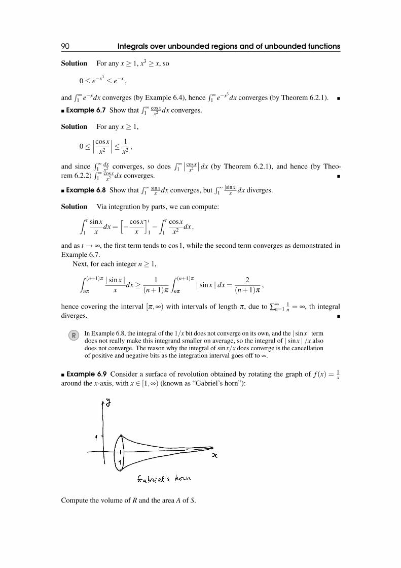
90 Integrals over unbounded regions and of unbounded functions
Solution For any x≥ 1, x3 ≥ x, so
0≤ e−x3 ≤ e−x ,
and∫
∞
1 e−xdx converges (by Example 6.4), hence∫
∞
1 e−x3dx converges (by Theorem 6.2.1). �
� Example 6.7 Show that∫
∞
1cosx
x2 dx converges.
Solution For any x≥ 1,
0≤∣∣∣cosx
x2
∣∣∣≤ 1x2 ,
and since∫
∞
1dxx2 converges, so does
∫∞
1
∣∣ cosxx2
∣∣dx (by Theorem 6.2.1), and hence (by Theo-rem 6.2.2)
∫∞
1cosx
x2 dx converges. �
� Example 6.8 Show that∫
∞
1sinx
x dx converges, but∫
∞
1|sinx|
x dx diverges.
Solution Via integration by parts, we can compute:∫ t
1
sinxx
dx =[−cosx
x
]t
1−∫ t
1
cosxx2 dx ,
and as t→ ∞, the first term tends to cos1, while the second term converges as demonstrated inExample 6.7.
Next, for each integer n≥ 1,∫ (n+1)π
nπ
| sinx |x
dx≥ 1(n+1)π
∫ (n+1)π
nπ
| sinx | dx =2
(n+1)π,
hence covering the interval [π,∞) with intervals of length π , due to ∑∞n=1
1n = ∞, th integral
diverges. �
R In Example 6.8, the integral of the 1/x bit does not converge on its own, and the | sinx | termdoes not really make this integrand smaller on average, so the integral of | sinx | /x alsodoes not converge. The reason why the integral of sinx/x does converge is the cancellationof positive and negative bits as the integration interval goes off to ∞.
� Example 6.9 Consider a surface of revolution obtained by rotating the graph of f (x) = 1x
around the x-axis, with x ∈ [1,∞) (known as “Gabriel’s horn”):
Compute the volume of R and the area A of S.
6.3 Convergence of integrals – continued 91
Solution For the volume V of the solid R, we have
V = π
∫∞
1
1x2 dx .
This integral converges to V = π .For the area A of the surface S of the solid, we have
A = 2π
∫∞
1
1x
√1+
1x4 dx .
Since
1x
√1+
1x4 >
1x,
and since∫
∞
11x dx diverges, we conclude that the surface area of this solid diverges (i.e. is infinite).
�
R Note: The opposite (infinite volume, but finite surface area) is not possible, because forsurfaces of revolution,
V ≤ 12
R ·AS , (6.5)
where R is the largest radius and AS is the surface area.
� Example 6.10 Consider the integral
I =∫
∞
1
x3 +2x−37x5 +4x2 +8
dx .
Determine whether I converges.
Solution Since the only negative term is −37, it is clear that for large enough x the integrandis positive. Since the terms in the denominator are always positive,
x3 +2x−37x5 +4x2 +8
≤ x3 +2x−37x5 =
1x2 +
2x4 −
37x5 .
Since the integrals∫
∞
1dxx2 ,∫
∞
1dxx4 and
∫∞
1dxx5 all converge, by virtue of the Comparison Test I
converges. �
� Example 6.11 Investigate the divergence of
I =∫
∞
2
5x+3x3−1
dx .
Solution x3−1 for large x behaves as x3, while 5x+3 for large x behaves as 5x. Thus,
x3−15x+3
≈ 5x2 .
For x ≥ 2, x3− 1 > 0, so we can apply a Comparison Test to prove the convergence. Sincewe want to estimate the integrand from above, we want to put a suitable lower bound on thedenominator. Since for x≥ 2 we have x3
2 ≥ 4, we have
x3−1≥ x3−4≥ x3− x3
2=
x3
2.
92 Integrals over unbounded regions and of unbounded functions
Therefore,
5x+3x3−1
≤ 5x+3x3/2
=10x2 +
6x3 .
Since both∫
∞
210x2 dx and
∫∞
26x3 dx converge, by the Comparison Test I converges as well. �
� Example 6.12 Investigate the convergence of
I =∫
∞
2
x3/2 +4x2−1
.
Solution The integrand is positive for x≥ 2, thus we can apply a Comparison Test. We have
x3/2 +4x2−1
≥ x3/2 +4x2 =
1x1/2 +
4x2 .
Since∫
∞
2dx
x1/2 diverges,∫∞
2
(1
x1/2 +4x2
)dx
diverges, and thus by the Comparison Test I diverges as well. �
� Example 6.13 Investigate the convergence of
I =∫
∞
2
x3/2 +4x2 +1
.
Solution For x≥ 2, x2 ≥ 4. Therefore,
x2 +1≤ x2 +4≤ x2 + x2 = 2x2 ,
which leads to
x3/2 +4x2 +1
≤ x3/2 +42x2 =
12x1/2 +
2x2 .
Since∫
∞
2dx
x1/2 diverges,∫∞
2
(1
x1/2 +2x2
)dx
diverges, thus by the Comparison Test I diverges as well. �
6.4 Integrals of unbounded functionsWe now consider integrals
∫ ba f (x)dx, where f : (a,b]→ R or f : [a,b)→ R, but where f is
unbounded near the end point where it is not defined (e.g.∫ 1
01x dx). The following discussion of
integrals of unbounded functions is almost identical to the above discussion of integrals overunbounded domains.
Clearly, to integrate a function f : [a,b)→R over [a,b), we will need it to be integrable overany interval [a, t] with a < t < b.
6.5 Convergence tests for integrals of unbounded functions 93
Definition 6.4.1 Suppose that f : [a,b)→ R is integrable over [a, t] for any a < t < b. Thenthe integral
∫ ba f (x)dx is defined to be∫ B
af (x)dx := lim
t→b
∫ t
af (x)dx . (6.6)
If this limit exists and is finite, then we say that the integral converges, while if the limit doesnot exist or is infinite, we say that the integral diverges (and so does not have a value).
For a function f : (a,b]→ R, we define convergence and divergence of∫ b
a f (x)dx simi-larly.
� Example 6.14 Show that∫ 1
0 x−αdx converges iff α < 1.
Solution If α 6= 1, then
∫ 1
tx−αdx =
[(1−α)x1−α
]1t = (1−α)−1(1− t1−α)
t→0−−→{
(1−α)−1 if 1−α > 0∞ if 1−α < 0
,
so the integral converges to (1−α)−1 if α > 1, and it diverges α < 1.If α = 1, then∫ 1
t
dxx
= [lnx]1t =− ln t t→0−−→ ∞,
so the integral diverges. �
Note the difference with example 9.6
6.5 Convergence tests for integrals of unbounded functions
In this case we have similar convergence tests as in the previous case:
Theorem 6.5.1 — Comparison Test. Suppose that f .g : [a,b)→ R are integrable on [a,x]for all a < x < b, and suppose that there is a number c such that a < c < b and 0≤ g(x)≤ f (x)for all c≤ x≤ b. Then:(a)
∫ ba f converges⇒
∫ ba g converges;
(b)∫ b
a g diverges⇒∫ b
a f diverges.An analogous result holds for integrals over (a,b].
Theorem 6.5.2 — Absolute Convergence Test. Suppose that f : [a,b)→ R is integrableon [a,x] for all a < x < b. Then:∫ b
a| f | converges ⇒
∫ b
af converges.
An analogous result holds for integrals over (a,b].
� Example 6.15 Show that∫ 1
0sinx−1
x1/2 dx converges.
Solution The problem is at x = 0, but the proof is almost the same as in Example 6.7 �
� Example 6.16 Show that I =∫ 2
01
|x−1|α dx converges for 0≤ α < 1 and diverges for α ≥ 1.
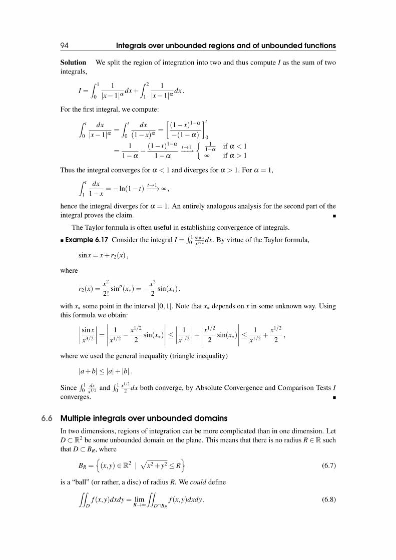
94 Integrals over unbounded regions and of unbounded functions
Solution We split the region of integration into two and thus compute I as the sum of twointegrals,
I =∫ 1
0
1|x−1|α
dx+∫ 2
1
1|x−1|α
dx .
For the first integral, we compute:∫ t
0
dx|x−1|α
=∫ t
0
dx(1− x)α
=
[(1− x)1−α
−(1−α)
]t
0
=1
1−α− (1− t)1−α
1−α
t→1−−→{ 1
1−αif α < 1
∞ if α > 1
Thus the integral converges for α < 1 and diverges for α > 1. For α = 1,∫ t
1
dx1− x
=− ln(1− t) t→1−−→ ∞ ,
hence the integral diverges for α = 1. An entirely analogous analysis for the second part of theintegral proves the claim. �
The Taylor formula is often useful in establishing convergence of integrals.
� Example 6.17 Consider the integral I =∫ 1
0sinxx3/2 dx. By virtue of the Taylor formula,
sinx = x+ r2(x) ,
where
r2(x) =x2
2!sin′′(x∗) =−
x2
2sin(x∗) ,
with x∗ some point in the interval [0,1]. Note that x∗ depends on x in some unknown way. Usingthis formula we obtain:∣∣∣∣sinx
x3/2
∣∣∣∣=∣∣∣∣∣ 1x1/2 −
x1/2
2sin(x∗)
∣∣∣∣∣≤∣∣∣∣ 1x1/2
∣∣∣∣+∣∣∣∣∣x1/2
2sin(x∗)
∣∣∣∣∣≤ 1x1/2 +
x1/2
2,
where we used the general inequality (triangle inequality)
|a+b| ≤ |a|+ |b| .
Since∫ 1
0dx
x1/2 and∫ 1
0x1/2
2 dx both converge, by Absolute Convergence and Comparison Tests Iconverges. �
6.6 Multiple integrals over unbounded domainsIn two dimensions, regions of integration can be more complicated than in one dimension. LetD⊂ R2 be some unbounded domain on the plane. This means that there is no radius R ∈ R suchthat D⊂ BR, where
BR ={(x,y) ∈ R2 |
√x2 + y2 ≤ R
}(6.7)
is a “ball” (or rather, a disc) of radius R. We could define∫∫D
f (x,y)dxdy = limR→∞
∫∫D∩BR
f (x,y)dxdy . (6.8)
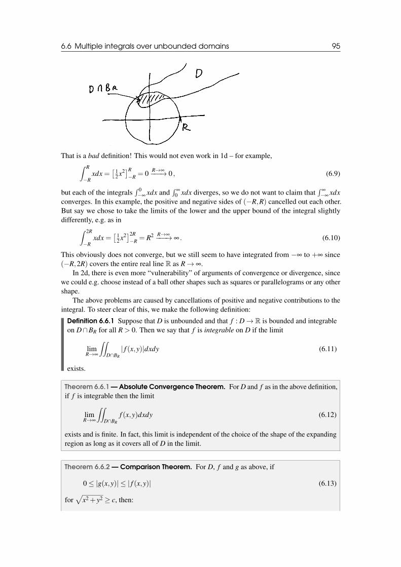
6.6 Multiple integrals over unbounded domains 95
That is a bad definition! This would not even work in 1d – for example,∫ R
−Rxdx =
[12 x2]R
−R = 0 R→∞−−−→ 0 , (6.9)
but each of the integrals∫ 0−∞
xdx and∫
∞
0 xdx diverges, so we do not want to claim that∫
∞
−∞xdx
converges. In this example, the positive and negative sides of (−R,R) cancelled out each other.But say we chose to take the limits of the lower and the upper bound of the integral slightlydifferently, e.g. as in∫ 2R
−Rxdx =
[12 x2]2R
−R = R2 R→∞−−−→ ∞ . (6.10)
This obviously does not converge, but we still seem to have integrated from −∞ to +∞ since(−R,2R) covers the entire real line R as R→ ∞.
In 2d, there is even more “vulnerability” of arguments of convergence or divergence, sincewe could e.g. choose instead of a ball other shapes such as squares or parallelograms or any othershape.
The above problems are caused by cancellations of positive and negative contributions to theintegral. To steer clear of this, we make the following definition:
Definition 6.6.1 Suppose that D is unbounded and that f : D→ R is bounded and integrableon D∩BR for all R > 0. Then we say that f is integrable on D if the limit
limR→∞
∫∫D∩BR
| f (x,y)|dxdy (6.11)
exists.
Theorem 6.6.1 — Absolute Convergence Theorem. For D and f as in the above definition,if f is integrable then the limit
limR→∞
∫∫D∩BR
f (x,y)dxdy (6.12)
exists and is finite. In fact, this limit is independent of the choice of the shape of the expandingregion as long as it covers all of D in the limit.
Theorem 6.6.2 — Comparison Theorem. For D, f and g as above, if
0≤ |g(x,y)| ≤ | f (x,y)| (6.13)
for√
x2 + y2 ≥ c, then:
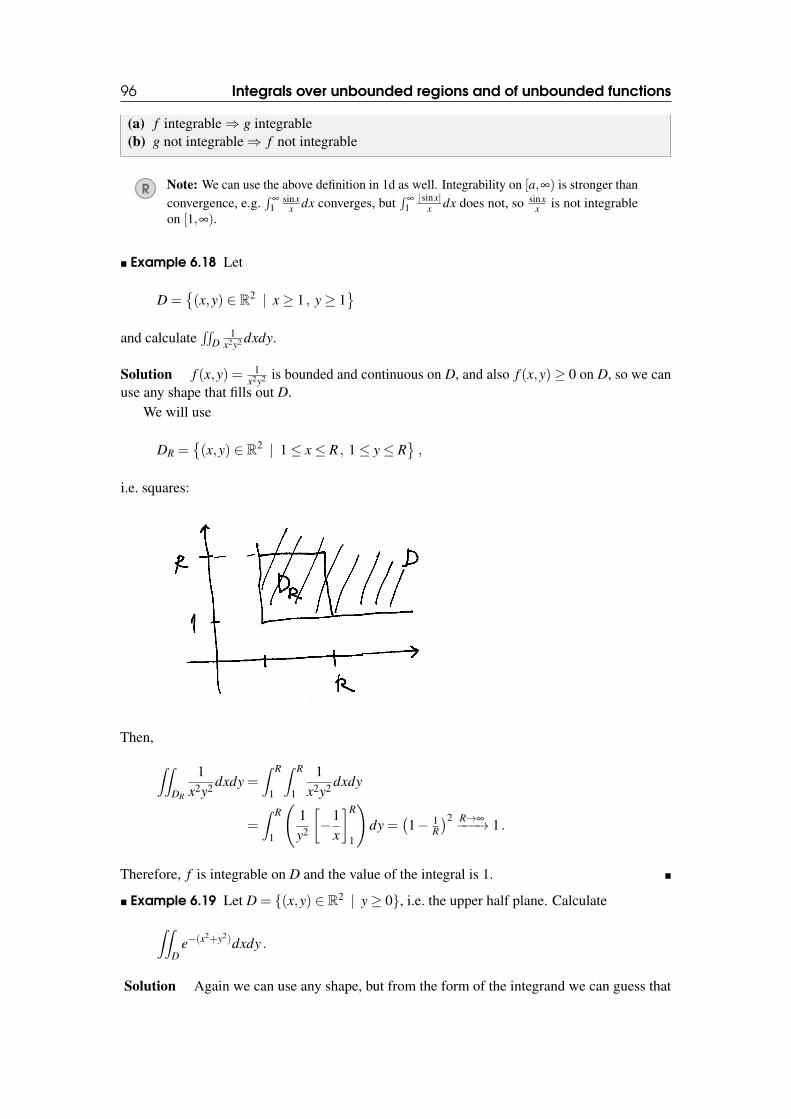
96 Integrals over unbounded regions and of unbounded functions
(a) f integrable⇒ g integrable(b) g not integrable⇒ f not integrable
R Note: We can use the above definition in 1d as well. Integrability on [a,∞) is stronger thanconvergence, e.g.
∫∞
1sinx
x dx converges, but∫
∞
1|sinx|
x dx does not, so sinxx is not integrable
on [1,∞).
� Example 6.18 Let
D ={(x,y) ∈ R2 | x≥ 1 , y≥ 1
}and calculate
∫∫D
1x2y2 dxdy.
Solution f (x,y) = 1x2y2 is bounded and continuous on D, and also f (x,y)≥ 0 on D, so we can
use any shape that fills out D.We will use
DR ={(x,y) ∈ R2 | 1≤ x≤ R , 1≤ y≤ R
},
i.e. squares:
Then,
∫∫DR
1x2y2 dxdy =
∫ R
1
∫ R
1
1x2y2 dxdy
=∫ R
1
(1y2
[−1
x
]R
1
)dy =
(1− 1
R
)2 R→∞−−−→ 1 .
Therefore, f is integrable on D and the value of the integral is 1. �
� Example 6.19 Let D = {(x,y) ∈ R2 | y≥ 0}, i.e. the upper half plane. Calculate
∫∫D
e−(x2+y2)dxdy .
Solution Again we can use any shape, but from the form of the integrand we can guess that
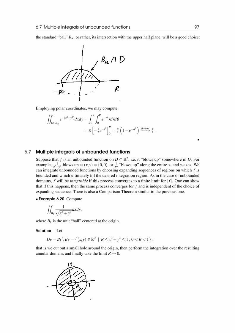
6.7 Multiple integrals of unbounded functions 97
the standard “ball” BR, or rather, its intersection with the upper half plane, will be a good choice:
Employing polar coordinates, we may compute:∫∫D∩BR
e−(x2+y2)dxdy =
∫π
0
∫ R
0e−r2
rdrdθ
= π
[−1
2 e−r2]R
0= π
2
(1− e−R2
)R→∞−−−→ π
2 .
�
6.7 Multiple integrals of unbounded functionsSuppose that f is an unbounded function on D ⊂ R2, i.e. it “blows up” somewhere in D. Forexample, 1
x2+y2 blows up at (x,y) = (0,0), or 1xy “blows up” along the entire x- and y-axes. We
can integrate unbounded functions by choosing expanding sequences of regions on which f isbounded and which ultimately fill the desired integration region. As in the case of unboundeddomains, f will be integrable if this process converges to a finite limit for | f |. One can showthat if this happens, then the same process converges for f and is independent of the choice ofexpanding sequence. There is also a Comparison Theorem similar to the previous one.
� Example 6.20 Compute∫∫B1
1√x2 + y2
dxdy ,
where B1 is the unit “ball” centered at the origin.
Solution Let
DR = B1 \BR ={(x,y) ∈ R2 | R≤ x2 + y2 ≤ 1 , 0 < R < 1
},
that is we cut out a small hole around the origin, then perform the integration over the resultingannular domain, and finally take the limit R→ 0.
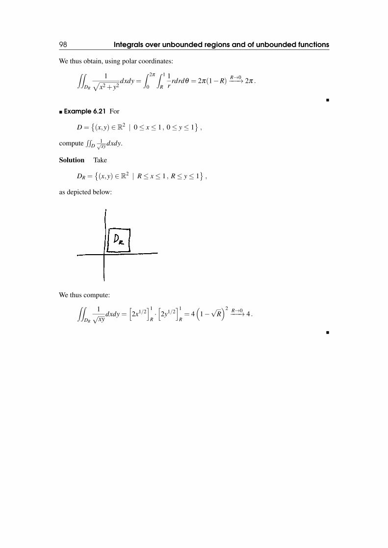
98 Integrals over unbounded regions and of unbounded functions
We thus obtain, using polar coordinates:∫∫DR
1√x2 + y2
dxdy =∫ 2π
0
∫ 1
R
1r
rdrdθ = 2π(1−R) R→0−−−→ 2π .
�
� Example 6.21 For
D ={(x,y) ∈ R2 | 0≤ x≤ 1 , 0≤ y≤ 1
},
compute∫∫
D1√xy dxdy.
Solution Take
DR ={(x,y) ∈ R2 | R≤ x≤ 1 , R≤ y≤ 1
},
as depicted below:
We thus compute:∫∫DR
1√
xydxdy =
[2x1/2
]1
R·[2y1/2
]1
R= 4
(1−√
R)2 R→0−−−→ 4 .
�
Maxima and minimaSecond derivative test for maxima andminima – one variable case
Second derivative test for two variablesLagrange multipliersMore examples
7 — More applications of partial derivatives
7.1 Maxima and minima
Let f : R3→ R. It is said that f has a global
minimummaximum
at (x0,y0) iff (x0,y0)≤ f (x,y)f(x0,y0)≥ f (x,y)
for all (x,y) ∈ R2. It is said that f has a local
minimummaximum
at (x0,y0) iff (x0,y0)≤ f (x,y)f(x0,y0)≥ f (x,y)
for all (x,y) in a neighborhood of (x0,y0).
� Example 7.1 Let f be the height function defined on the Scottish highlands. Then the top ofevery mountain is a local maximum (i.e. all nearby points are lower). The top of Ben Nevis isthe global maximum. �
Recall that for f : R1→ R1, f ′ = 0 at any local maximum or minimum.
The converse need not be true. For example, the function f (x) = x3 has an inflection point at the
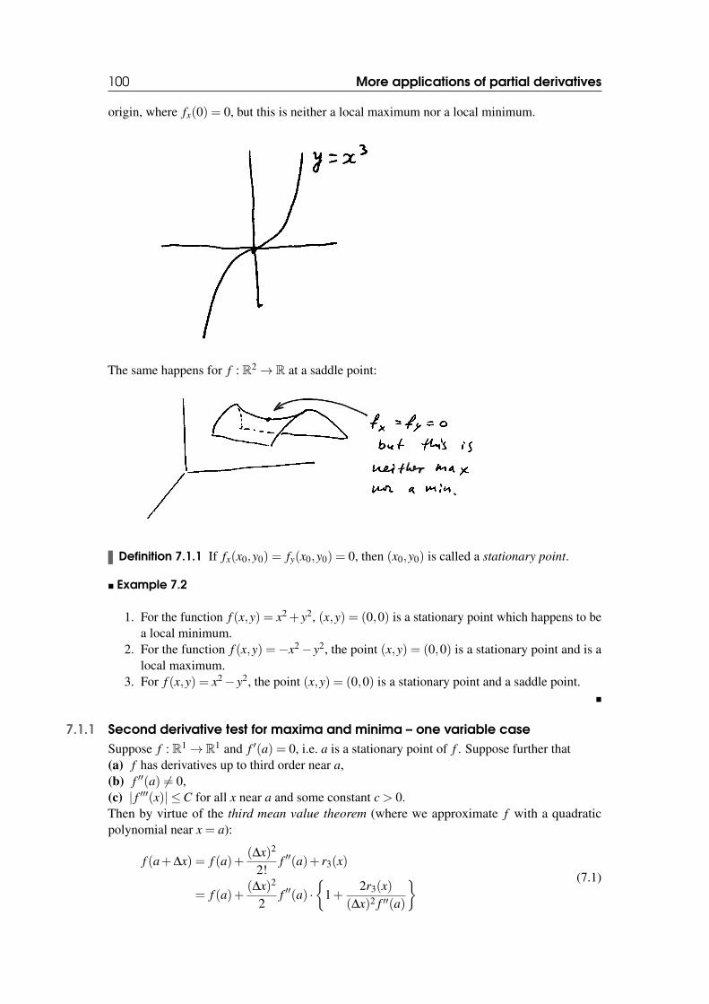
100 More applications of partial derivatives
origin, where fx(0) = 0, but this is neither a local maximum nor a local minimum.
The same happens for f : R2→ R at a saddle point:
Definition 7.1.1 If fx(x0,y0) = fy(x0,y0) = 0, then (x0,y0) is called a stationary point.
� Example 7.2
1. For the function f (x,y) = x2 + y2, (x,y) = (0,0) is a stationary point which happens to bea local minimum.
2. For the function f (x,y) =−x2− y2, the point (x,y) = (0,0) is a stationary point and is alocal maximum.
3. For f (x,y) = x2− y2, the point (x,y) = (0,0) is a stationary point and a saddle point.�
7.1.1 Second derivative test for maxima and minima – one variable caseSuppose f : R1→ R1 and f ′(a) = 0, i.e. a is a stationary point of f . Suppose further that(a) f has derivatives up to third order near a,(b) f ′′(a) 6= 0,(c) | f ′′′(x)| ≤C for all x near a and some constant c > 0.Then by virtue of the third mean value theorem (where we approximate f with a quadraticpolynomial near x = a):
f (a+∆x) = f (a)+(∆x)2
2!f ′′(a)+ r3(x)
= f (a)+(∆x)2
2f ′′(a) ·
{1+
2r3(x)(∆x)2 f ′′(a)
} (7.1)
7.2 Second derivative test for two variables 101
We may estimate the remainder term (cf. Thoerem 3.6.1)
r3(x) =(∆x)3 f ′′′(x∗)
3!,
as
|r3(x)| ≤|∆x|3 · c
6,
hence:∣∣∣∣ 2r3(x)(∆x)2 f ′′(a)
∣∣∣∣≤ 2|∆x|3 · c6(∆x)2| f ′′(a)|
=c
3| f ′′(a)|· |∆x|< 1 if |∆x|< 3| f ′′(a)|
c.
Thus, for sufficiently small ∆x the term {. . .} in (7.1) above is positive, hence if
f ′′(a)< 0 ⇒ x = a is a local maximum
f ′′(a)> 0 ⇒ x = a is a local minimum .
7.2 Second derivative test for two variablesLet f : R2→ R1 and fx(a,b) = fy(a,b) = 0, i.e. (a,b) is a stationary point. Taylor’s formulareveals that
f (a+∆x,b+∆y) = f (a,b)+12
Q(∆x,∆y)+R3(x,y) , (7.2)
where
Q(∆x,∆y) = A · (∆x)2 +2B∆x∆y+C · (∆y)2
A = fxx(a,b) , B = fxy(a,b) , C = fyy(a,b) .
We will ignore the remainder term R3(x,y) below. It can be shown similarly to the one variablecase that under certain assumptions one can indeed neglect R3(x,y). We distinguish three specialcases:• If Q(∆x,∆y)< 0 for all sufficiently small ∆x, ∆y, then (a,b) is a local maximum.• If Q(∆x,∆y)> 0 for all sufficiently small ∆x, ∆y, then (a,b) is a local minimum.• If Q(∆x,∆y) can take both positive and negative values for all sufficiently small ∆x, ∆y,
then (a,b) is a saddle point.In the special case Q(∆x,∆y) = 0 for all sufficiently small ∆x, ∆y, the remainder term R3(x,y)has to be analyzed.
Assume that A 6= 0. Then, we can rewrite Q as
Q(∆x,∆y) = A((∆x)2 +
2BA
∆x∆y+CA(∆y)2
)= A
((∆x+
BA
∆y)2
+
(CA− B2
A2
)(∆y)2
)
= A((
∆x+BA
∆y)2
︸ ︷︷ ︸≥0
+(AC−B2)(∆y)2
A2︸ ︷︷ ︸≥0
).
(7.3)
102 More applications of partial derivatives
Thus:(a) If AC−B2 > 0, then Q has the same sign as A for all (sufficiently small) ∆x and ∆y. We may
discern the following cases:• AC−B2 > 0 and A < 0⇒ (a,b) is a local maximum• AC−B2 > 0 and A > 0⇒ (a,b) is a local minimum.
(b) If AC−B2 < 0, consider
Q(∆x,0) = A(∆x)2 .
It has the same sign as A. On the other hand,
Q(−B
A∆y,∆y
)= A · (AC−B2)︸ ︷︷ ︸
≤0
·(
∆yA
)2
︸ ︷︷ ︸≥0
has the sign opposite to the sign of A. Hence we conclude that if AC−B2 < 0, we have asaddle point.
R Notes:(a) If AC−B2 > 0, then AC > B2 ≥ 0, hence if A and C are not equal to 0 then A and C
have the same sign in this case. Hence we can look at the sign of C in the above test.(b) If A = 0 and C 6= 0, we can obtain a similar test by by dividing over C and completing
the square. If B 6= 0, in this case we have that
AC−B2 =−B2 < 0 ,
thus we have found a saddle point. A similar argument holds for the case A 6= 0,C = 0 and B 6= 0. In the case A = B = 0 but C 6= 0, we have for C > 0 a localminimum and for C < 0 a local maximum.
(c) If A =C = 0 and b 6= 0,
Q(∆x,∆y) = 2B∆x∆y
clearly changes sign, so we have a saddle point.(d) In the special case A = B =C = 0, the test does not work!
� Example 7.3 Find the stationary points of the following functions and determine their nature:(i) f (x,y) = 2x2− xy+ y2 +7x(ii) g(x,y) = xy− x3y− xy3.
Solution (i) fx = 4x− y+7, fy =−x+2y. A point (x,y) is a stationary point if
4x− y+7 = 0−x+2y = 0
}⇔ y = x
27x+14 = 0
}⇔ x =−2 and y =−1 .
Hence, (x,y) = (−2,−1) is the only stationary point.
Next, we calculate:
fxx = 4 , fxy =−1 fyy = 2 ,
from which we conclude that
AC−B2 = fxx · fyy− ( fxy)2 = 4 ·21 = 7 > 0 .
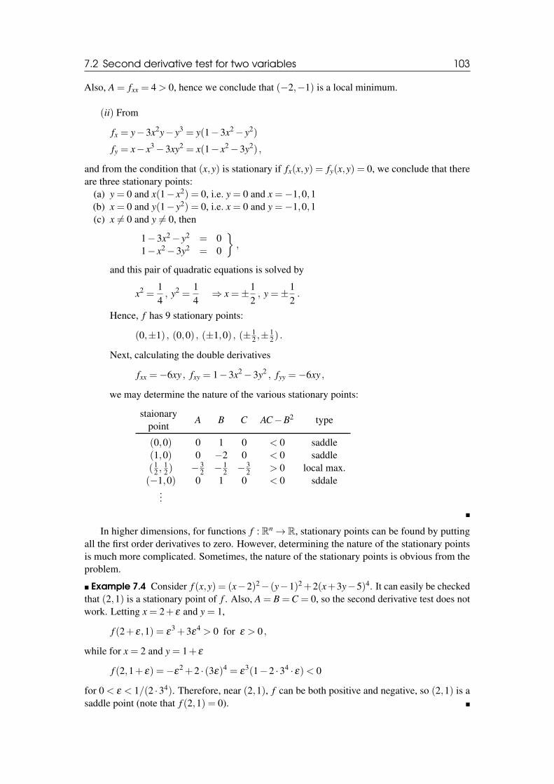
7.2 Second derivative test for two variables 103
Also, A = fxx = 4 > 0, hence we conclude that (−2,−1) is a local minimum.
(ii) From
fx = y−3x2y− y3 = y(1−3x2− y2)
fy = x− x3−3xy2 = x(1− x2−3y2) ,
and from the condition that (x,y) is stationary if fx(x,y) = fy(x,y) = 0, we conclude that thereare three stationary points:
(a) y = 0 and x(1− x2) = 0, i.e. y = 0 and x =−1,0,1(b) x = 0 and y(1− y2) = 0, i.e. x = 0 and y =−1,0,1(c) x 6= 0 and y 6= 0, then
1−3x2− y2 = 01− x2−3y2 = 0
},
and this pair of quadratic equations is solved by
x2 =14, y2 =
14⇒ x =±1
2, y =±1
2.
Hence, f has 9 stationary points:
(0,±1) , (0,0) , (±1,0) , (±12 ,±
12) .
Next, calculating the double derivatives
fxx =−6xy , fxy = 1−3x2−3y2 , fyy =−6xy ,
we may determine the nature of the various stationary points:
staionarypoint
A B C AC−B2 type
(0,0) 0 1 0 < 0 saddle(1,0) 0 −2 0 < 0 saddle(1
2 ,12) −3
2 −12 −3
2 > 0 local max.(−1,0) 0 1 0 < 0 sddale
...
�
In higher dimensions, for functions f : Rn→ R, stationary points can be found by puttingall the first order derivatives to zero. However, determining the nature of the stationary pointsis much more complicated. Sometimes, the nature of the stationary points is obvious from theproblem.
� Example 7.4 Consider f (x,y) = (x−2)2− (y−1)2+2(x+3y−5)4. It can easily be checkedthat (2,1) is a stationary point of f . Also, A = B =C = 0, so the second derivative test does notwork. Letting x = 2+ ε and y = 1,
f (2+ ε,1) = ε3 +3ε
4 > 0 for ε > 0 ,
while for x = 2 and y = 1+ ε
f (2,1+ ε) =−ε2 +2 · (3ε)4 = ε
3(1−2 ·34 · ε)< 0
for 0 < ε < 1/(2 ·34). Therefore, near (2,1), f can be both positive and negative, so (2,1) is asaddle point (note that f (2,1) = 0). �
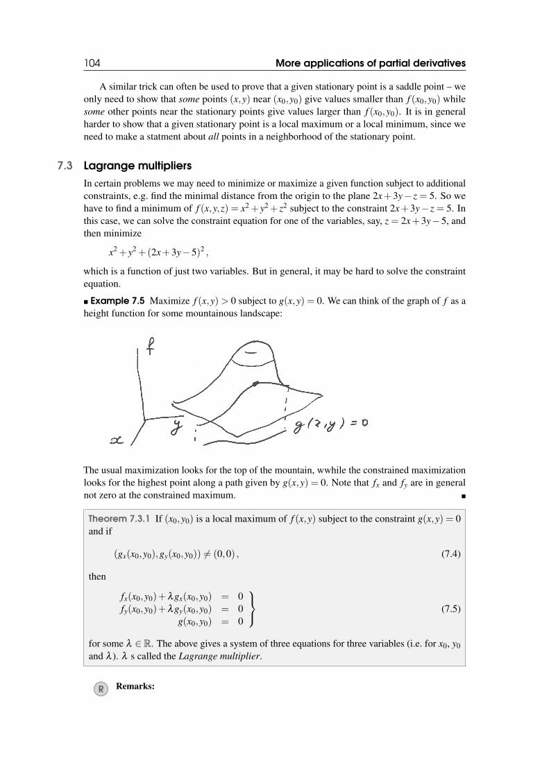
104 More applications of partial derivatives
A similar trick can often be used to prove that a given stationary point is a saddle point – weonly need to show that some points (x,y) near (x0,y0) give values smaller than f (x0,y0) whilesome other points near the stationary points give values larger than f (x0,y0). It is in generalharder to show that a given stationary point is a local maximum or a local minimum, since weneed to make a statment about all points in a neighborhood of the stationary point.
7.3 Lagrange multipliersIn certain problems we may need to minimize or maximize a given function subject to additionalconstraints, e.g. find the minimal distance from the origin to the plane 2x+3y− z = 5. So wehave to find a minimum of f (x,y,z) = x2 + y2 + z2 subject to the constraint 2x+3y− z = 5. Inthis case, we can solve the constraint equation for one of the variables, say, z = 2x+3y−5, andthen minimize
x2 + y2 +(2x+3y−5)2 ,
which is a function of just two variables. But in general, it may be hard to solve the constraintequation.
� Example 7.5 Maximize f (x,y)> 0 subject to g(x,y) = 0. We can think of the graph of f as aheight function for some mountainous landscape:
The usual maximization looks for the top of the mountain, wwhile the constrained maximizationlooks for the highest point along a path given by g(x,y) = 0. Note that fx and fy are in generalnot zero at the constrained maximum. �
Theorem 7.3.1 If (x0,y0) is a local maximum of f (x,y) subject to the constraint g(x,y) = 0and if
(gx(x0,y0),gy(x0,y0)) 6= (0,0) , (7.4)
then
fx(x0,y0)+λgx(x0,y0) = 0fy(x0,y0)+λgy(x0,y0) = 0
g(x0,y0) = 0
(7.5)
for some λ ∈R. The above gives a system of three equations for three variables (i.e. for x0, y0and λ ). λ s called the Lagrange multiplier.
R Remarks:
7.3 Lagrange multipliers 105
(1) If f ,g : Rn→ R, a similar system of n+1 equations can be written:
∂ f∂xi
(x0)+λ∂g∂xi
(x0) = 0 , i = 1, . . . ,n
y = y(x)
∂
∂x( f (x,y)+λg(x,y)) = 0
∂
∂y( f (x,y)+λg(x,y)) = 0
We can prove the above statement via applying the chain rule for differentiation:
ddx
( f (x,y(x))+λg(x,y(x))) = 0
⇔ fx(x,y(x))+λgx(x,y(x))+dydx
( fy(x,y(x))+λgy(x,y(x))) = 0
Thus, choosing λ ∈ R such that fy +λgy = 0, we obtain indeed that fx +λgx = 0.(2) If x0, y0 and λ do satisfy the above equations, there is no easy way (test) for determin-
ing the nature of the point, i.e. whether it is a local maximum, a local minimum or asaddle point.
(3) The first two equations are equivalent to looking for a stationary point of
h = f +λg .
� Example 7.6 Minimize f = x2 + y2 + z2 subject to the constraint 2x+3y− z = 5 and usingthe method of the Lagrange multiplier.
Solution Put
h(x,y,z) = x2 + y2 + z2 +λ (2x+3Y − z−5) .
Then we obtain the equation system
hx = 2x+2λ = 0hy = 2y+3λ = 0hz = 2z−λ = 0
2x+3y− z−5 = 0
.
Hence
x =−λ , y =−32
λ , z =−λ
2.
Substituting this into the last equation we ebtain:
2(−λ )+3(−32 λ )− (1
2 λ )−5 = 0
⇒ −7λ = 5
⇒ λ =−57,
and therefore the minimum occours at
(x,y,z) =(
57,1514
,− 514
),
and the minimal distance is√(57
)2
+
(1514
)2
+
(− 5
14
)2
=5√14
.
�
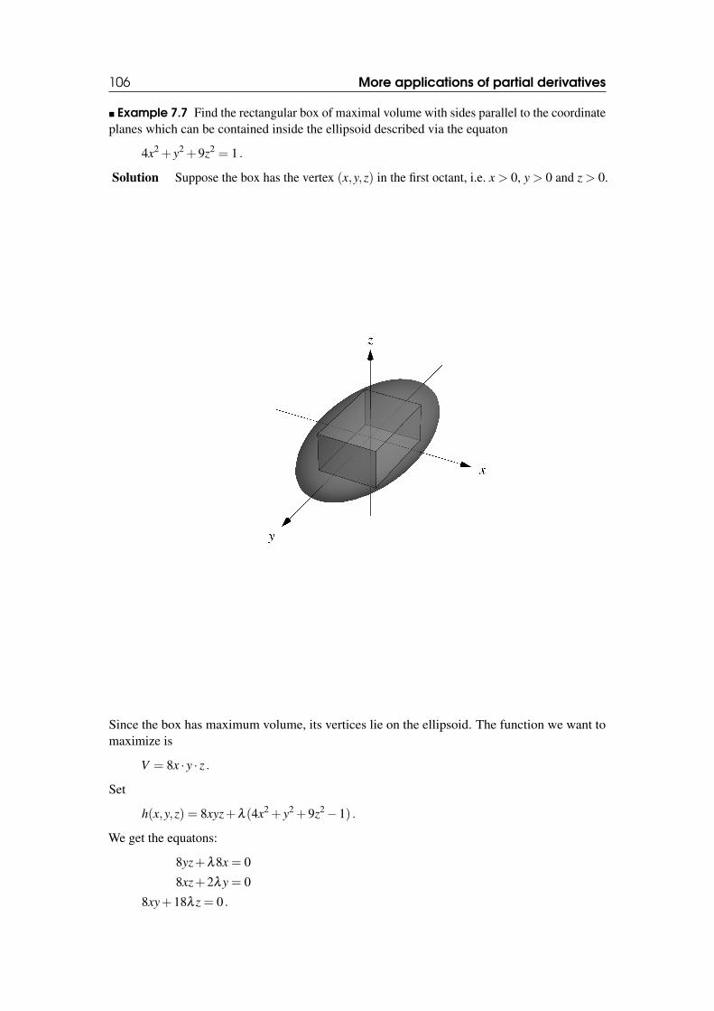
106 More applications of partial derivatives
� Example 7.7 Find the rectangular box of maximal volume with sides parallel to the coordinateplanes which can be contained inside the ellipsoid described via the equaton
4x2 + y2 +9z2 = 1 .
Solution Suppose the box has the vertex (x,y,z) in the first octant, i.e. x > 0, y > 0 and z > 0.
Since the box has maximum volume, its vertices lie on the ellipsoid. The function we want tomaximize is
V = 8x · y · z .
Set
h(x,y,z) = 8xyz+λ (4x2 + y2 +9z2−1) .
We get the equatons:
8yz+λ8x = 0
8xz+2λy = 0
8xy+18λ z = 0 .
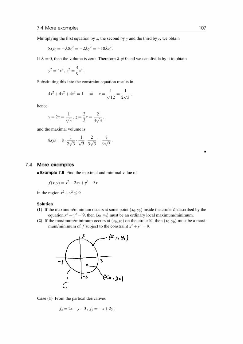
7.4 More examples 107
Multiplying the first equation by x, the second by y and the third by z, we obtain
8xyz =−λ8z2 =−2λy2 =−18λ z2 .
If λ = 0, then the volume is zero. Therefore λ 6= 0 and we can divide by it to obtain
y2 = 4x2 , z2 =49
x2 .
Substituting this into the constraint equation results in
4x2 +4x2 +4x2 = 1 ⇔ x =1√12
=1
2√
3,
hence
y = 2x =1√3, z =
23
x =2
3√
3,
and the maximal volume is
8xyz = 8 · 12√
3· 1√
3· 2
3√
3=
89√
3.
�
7.4 More examples� Example 7.8 Find the maximal and minimal value of
f (x,y) = x2−2xy+ y2−3x
in the region x2 + y2 ≤ 9.
Solution(1) If the maximum/minimum occurs at some point (x0,y0) inside the circle C described by the
equation x2 + y2 = 9, then (x0,y0) must be an ordinary local maximum/minimum.(2) If the maximum/minimum occurs at (x0,y0) on the circle C , then (x0,y0) must be a maxi-
mum/minimum of f subject to the constraint x2 + y2 = 9.
Case (1) From the partical derivatives
fx = 2x− y−3 , fy =−x+2y ,
108 More applications of partial derivatives
we may compute{2x− y−3 = 0−x+2y = 0
⇒ x = 2 , y = 1 .
The nature of this stationary point may be determined as follows:
fxx = 2 , fxy =−1 , fyy = 2f (2,1) =−3
⇒ fxx · fyy− ( fxy)2 = 3 > 0
fxx > 0.
Thus, (2,1) is a local minimum.Case (2) With
h(x,y) = x2− xy+ y2−3x+λ (x2 + y2−9)
hx = 2x− y−3+2λx = 0
hy =−x+2y+2λy = 0 ,
multiplying the first equation by y and the second equation by x and then taking thedifference, we can get rid of λ :
2xy− y2−3y− (−x2 +2xy) = 0 ⇔ x2 = y2 +3y .
Combining this with the constraint equation
x2 + y2 = 9 ,
we obtain
2y2 = 3y = 9 ⇔ (2y−3)(y+3) = 0 ⇔ y =32
or y =−3 .
Solving for x,
y =32⇒ x2 = 9− 9
4=
274
⇒ x =±3√
32
y =−3 ⇒ x = 0 ,
we conclude that the possible maxima/minima on the circle C are (±3√
32 , 3
2) and (0,−3).Together with the local minimum (2,1) computed previously, we have
f (2,1) =−3
f (0,−3) = 9
f (3√
32 , 3
2) = 9− 27√
32≈−2.69
f (−3√
32 , 3
2) = 9+27√
32≈ 20.69
Hence the maximum of f is ≈ 20.69 and is achieved at (−3√
32 , 3
2), while the minimum is−3 at (2,1).
�
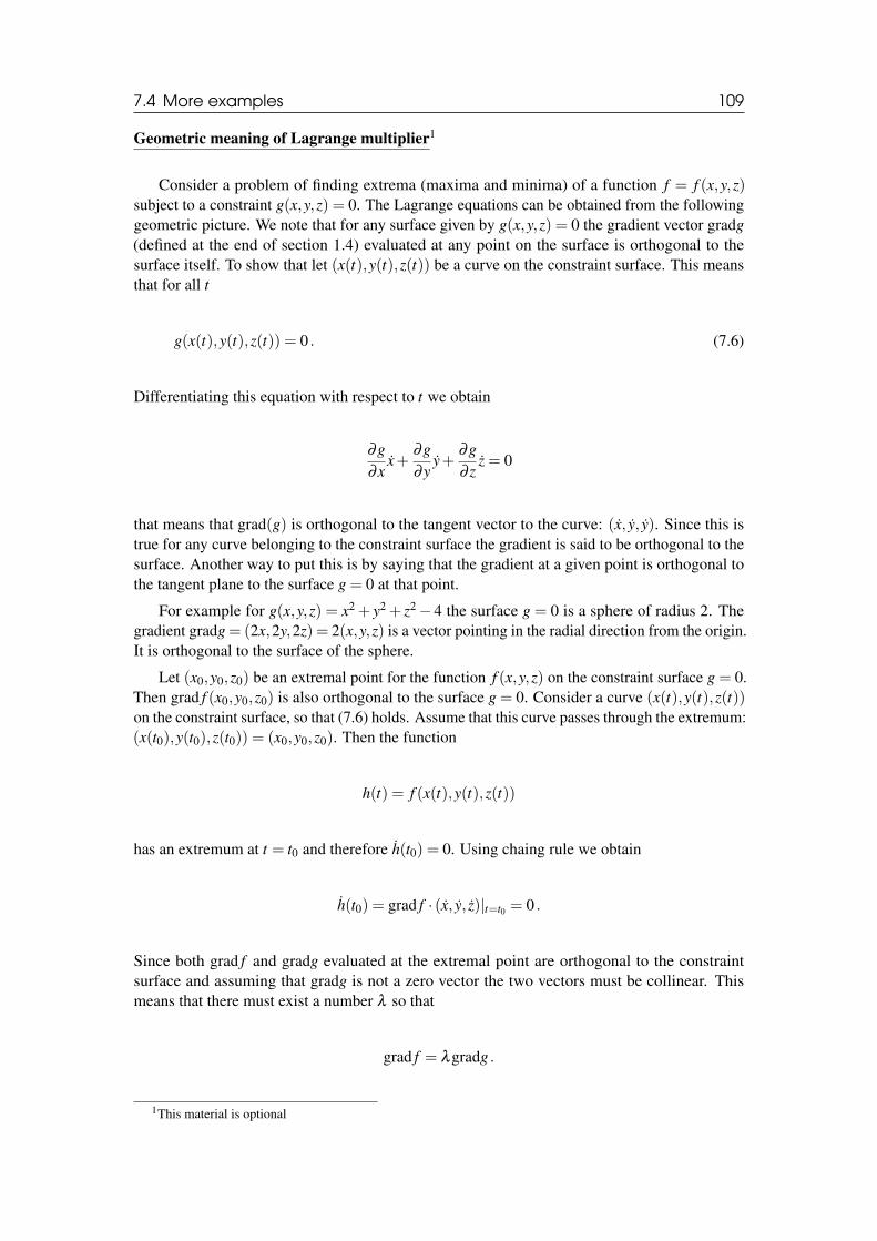
7.4 More examples 109
Geometric meaning of Lagrange multiplier1
Consider a problem of finding extrema (maxima and minima) of a function f = f (x,y,z)subject to a constraint g(x,y,z) = 0. The Lagrange equations can be obtained from the followinggeometric picture. We note that for any surface given by g(x,y,z) = 0 the gradient vector gradg(defined at the end of section 1.4) evaluated at any point on the surface is orthogonal to thesurface itself. To show that let (x(t),y(t),z(t)) be a curve on the constraint surface. This meansthat for all t
g(x(t),y(t),z(t)) = 0 . (7.6)
Differentiating this equation with respect to t we obtain
∂g∂x
x+∂g∂y
y+∂g∂ z
z = 0
that means that grad(g) is orthogonal to the tangent vector to the curve: (x, y, y). Since this istrue for any curve belonging to the constraint surface the gradient is said to be orthogonal to thesurface. Another way to put this is by saying that the gradient at a given point is orthogonal tothe tangent plane to the surface g = 0 at that point.
For example for g(x,y,z) = x2 + y2 + z2−4 the surface g = 0 is a sphere of radius 2. Thegradient gradg = (2x,2y,2z) = 2(x,y,z) is a vector pointing in the radial direction from the origin.It is orthogonal to the surface of the sphere.
Let (x0,y0,z0) be an extremal point for the function f (x,y,z) on the constraint surface g = 0.Then grad f (x0,y0,z0) is also orthogonal to the surface g = 0. Consider a curve (x(t),y(t),z(t))on the constraint surface, so that (7.6) holds. Assume that this curve passes through the extremum:(x(t0),y(t0),z(t0)) = (x0,y0,z0). Then the function
h(t) = f (x(t),y(t),z(t))
has an extremum at t = t0 and therefore h(t0) = 0. Using chaing rule we obtain
h(t0) = grad f · (x, y, z)|t=t0 = 0 .
Since both grad f and gradg evaluated at the extremal point are orthogonal to the constraintsurface and assuming that gradg is not a zero vector the two vectors must be collinear. Thismeans that there must exist a number λ so that
grad f = λgradg .
1This material is optional
110 More applications of partial derivatives
These are the first 3 Lagrange equations to which we must add the constraint equation g = 0.
Recommended books
There are many excellent calculus and analysis books. We recommend the book by John. B.Fraleigh "Calculus with analytic geometry" (any edition) that covers calculus and some analysisfor functions of one variable and also some topics (but not all that are covered in this notes) ofmultivariable calculus.
Another very useful book which has a large overlap with the material in the present notes isthe book by S. Lang "Calculus of several variables" (any edition). This book also coveres manyelements of vector analysis and may be useful in the 3rd year Vector analysis course.
If you want to go deeper into calculus and analysis of one and many variables an all timeclassic is "A course of pure mathematics" by G. H. Hardy.

Index
Analysis, 7Applications of double integrals, 65
Change of variables in double integrals, 66Change of variables in triple integrals, 77Continuity, 22Convergence of integrals, 87
convergence tests for integrals over un-bounded intervals, 89
integrals over unbounded intervals, 87Convergence tests for integrals of unbounded
functions, 93Coordinate systems
cylindrical polar coordinates, 77spherical polar coordinates, 80
DefinitionsC1-class function, 41(un)bounded intervals, 87(un-)bounded sequences, 11Continuity, 23convergence of sequences, 11differentiability
C1, 48differentiability and total derivative, 47Domain of a function, 20Graph of a function, 27integrability of functions, 95Partial derivatives, 25sequences, 10solution function, 41stationary point, 100Tangent plane, 29
Differentiation, 25
Functions f : Rm→ Rn, 46Functions of several variables, 19
Graphs, 27
Higher order partial derivatives, 33
Implicit differentiation, 42implicit differentiation formula, 42Implicit functions, 41Integrals of unbounded functions, 92Integrals over infinite regions, 87Interchanging the integrtion order, 63iterated integral, 60
Jacobian, 66
Lagrange multipliers, 104Limits of functions, 16Limits of sequences, 11
Maxima and minima, 99Multiple integrals, 59Multiple integrals of unbounded functions, 97Multiple integrals over unbounded domains,
94
Other substitutions, 70
RemindersDomains of some elementary functions,
19
114 INDEX
Second derivative test for maxima and min-ima, 100
Second derivative test for two variables, 101Sequences, 10
Tangent planes, 27Taylor’s expansion, 51Taylor’s formula in two dimensions, 56The chain rule and partial derivatives, 36Theorem
Comparison Theorem, 95Theorems
nth mean value theorem, 52Absolute Convergence Test, 89, 93Absolute Convergence Theorem, 95any convergent sequence is bounded, 13chain rule
general case, 49two variable case, 36
Comparison Test, 89, 93Criterion for differentiability of f : Rn→ Rm,
48implicit function theorem, 43
general case, 50three variable case, 44
Lagrange multiplier, 104Taylor’s formula in two dimensions, 56The implicit function theorem
two defining equations, 45The mixed derivatives theorem, 33
Total derivatives, 46Transforming equations, 38Triple integrals, 73
Various theorems about total derivatives, 49Volumes of revolution, 85