1

Physics 181

Notes on Multivariable Calculus

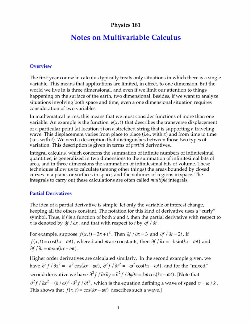
Overview The first year course in calculus typically treats only situations in which there is a single variable. This means that applications are limited, in effect, to one dimension. But the world we live in is three dimensional, and even if we limit our attention to things happening on the surface of the earth, two dimensional. Besides, if we want to analyze situations involving both space and time, even a one dimensional situation requires consideration of two variables. In mathematical terms, this means that we must consider functions of more than one variable. An example is the function

y(x,t) that describes the transverse displacement

of a particular point (at location x) on a stretched string that is supporting a traveling wave. This displacement varies from place to place (i.e., with x) and from time to time (i.e., with t). We need a description that distinguishes between those two types of variation. This description is given in terms of partial derivatives. Integral calculus, which concerns the summation of infinite numbers of infinitesimal quantities, is generalized in two dimensions to the summation of infinitesimal bits of area, and in three dimensions the summation of infinitesimal bits of volume. These techniques allow us to calculate (among other things) the areas bounded by closed curves in a plane, or surfaces in space, and the volumes of regions in space. The integrals to carry out these calculations are often called multiple integrals. Partial Derivatives The idea of a partial derivative is simple: let only the variable of interest change, keeping all the others constant. The notation for this kind of derivative uses a “curly” symbol. Thus, if f is a function of both x and t, then the partial derivative with respect to x is denoted by

!f /!x , and that with respect to t by !f /!t .

For example, suppose f (x,t) = 3x + t2 . Then

!f /!x = 3 and !f /!t = 2t . If

f (x,t) = cos(kx !"t) , where k and ω are constants, then !f /!x = "ksin(kx "#t) and

!f /!t =" sin(kx #"t) .

Higher order derivatives are calculated similarly. In the second example given, we have

!2 f /!x2

= "k2 cos(kx "#t) , !

2 f /!t2= "#

2 cos(kx "#t) , and for the “mixed”

second derivative we have !

2 f /!x!y = !2 f /!y!x = k" cos(kx #"t) . [Note that

!2 f /!x2

= (k/" )2# !

2 f /!t2 , which is the equation defining a wave of speed v =! /k . This shows that

f (x,t) = cos(kx !"t) describes such a wave.]

2

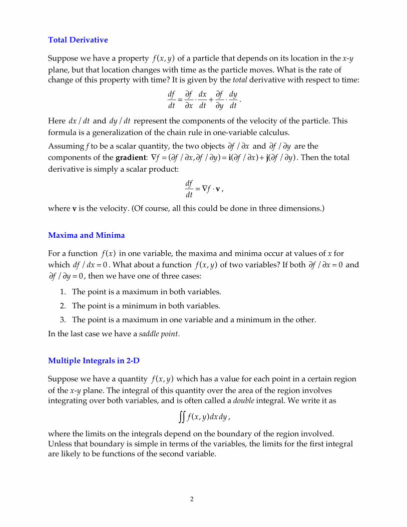
Total Derivative Suppose we have a property

f (x, y) of a particle that depends on its location in the x-y plane, but that location changes with time as the particle moves. What is the rate of change of this property with time? It is given by the total derivative with respect to time:

df

dt=!f

!x"dx

dt+!f

!y"dy

dt.

Here dx/dt and dy/dt represent the components of the velocity of the particle. This

formula is a generalization of the chain rule in one-variable calculus. Assuming f to be a scalar quantity, the two objects

!f /!x and !f /!y are the

components of the gradient: !f = ("f /"x,"f /"y) = i("f /"x) + j("f /"y) . Then the total

derivative is simply a scalar product:

df

dt= !f "v ,

where v is the velocity. (Of course, all this could be done in three dimensions.) Maxima and Minima For a function

f (x) in one variable, the maxima and minima occur at values of x for which

df /dx = 0 . What about a function f (x, y) of two variables? If both

!f /!x = 0 and

!f /!y = 0 , then we have one of three cases:

1. The point is a maximum in both variables.

2. The point is a minimum in both variables. 3. The point is a maximum in one variable and a minimum in the other.

In the last case we have a saddle point. Multiple Integrals in 2-D Suppose we have a quantity

f (x, y) which has a value for each point in a certain region of the x-y plane. The integral of this quantity over the area of the region involves integrating over both variables, and is often called a double integral. We write it as

f (x, y)dxdy!! ,

where the limits on the integrals depend on the boundary of the region involved. Unless that boundary is simple in terms of the variables, the limits for the first integral are likely to be functions of the second variable.

3

Examples.

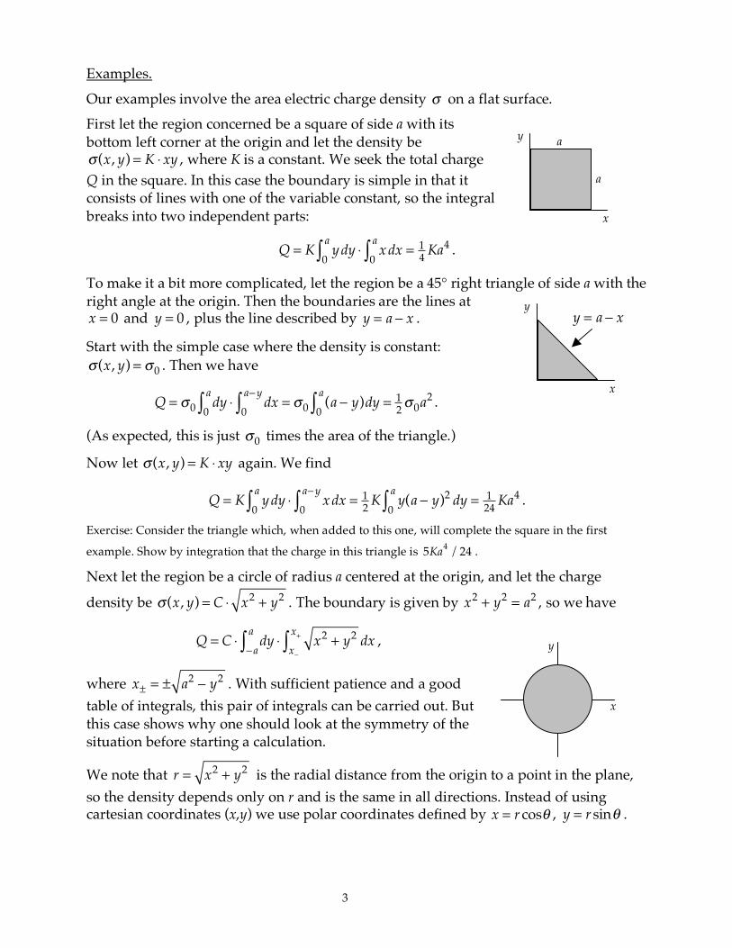
Our examples involve the area electric charge density ! on a flat surface. First let the region concerned be a square of side a with its bottom left corner at the origin and let the density be ! (x, y) = K " xy , where K is a constant. We seek the total charge Q in the square. In this case the boundary is simple in that it consists of lines with one of the variable constant, so the integral breaks into two independent parts:

Q = K ydy

0

a

! " xdx0

a

! =1

4Ka4 .

To make it a bit more complicated, let the region be a 45° right triangle of side a with the right angle at the origin. Then the boundaries are the lines at x = 0 and

y = 0 , plus the line described by

y = a ! x .

Start with the simple case where the density is constant:

! (x, y) = !0 . Then we have

Q = !0 dy

0

a

" # dx0

a$y

" = !0 (a $ y)dy0

a

" =12!0a2 .

(As expected, this is just !

0 times the area of the triangle.)

Now let ! (x, y) = K " xy again. We find

Q = K ydy

0

a

! " x dx0

a#y

! =12

K y(a # y)2 dy0

a

! =124

Ka4 .

Exercise: Consider the triangle which, when added to this one, will complete the square in the first

example. Show by integration that the charge in this triangle is 5Ka4

/ 24 .

Next let the region be a circle of radius a centered at the origin, and let the charge

density be ! (x, y) = C " x2

+ y2 . The boundary is given by x2

+ y2= a2 , so we have

Q = C ! dy

"a

a

# ! x2+ y2 dx

x"

x+

# ,

where x±= ± a2

! y2 . With sufficient patience and a good table of integrals, this pair of integrals can be carried out. But this case shows why one should look at the symmetry of the situation before starting a calculation.

We note that r = x2

+ y2 is the radial distance from the origin to a point in the plane, so the density depends only on r and is the same in all directions. Instead of using cartesian coordinates (x,y) we use polar coordinates defined by x = r cos! ,

y = r sin! .

y

x

y = a ! x

x

y

y

x

a

a

4

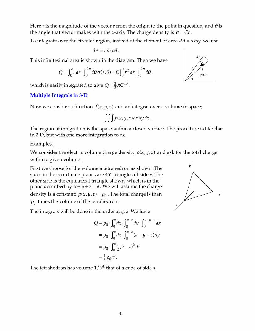
Here r is the magnitude of the vector r from the origin to the point in question, and θ is the angle that vector makes with the x-axis. The charge density is ! = Cr . To integrate over the circular region, instead of the element of area dA = dxdy we use

dA = r dr d! .

This infinitesimal area is shown in the diagram. Then we have

Q = r dr

0

a

! " d#0

2$

! % (r ,#) = C r2 dr0

a

! " d#0

2$

! ,

which is easily integrated to give Q =

2

3!Ca3 .

Multiple Integrals in 3-D Now we consider a function

f (x, y,z) and an integral over a volume in space;

f (x, y,z)dxdydz!!! .

The region of integration is the space within a closed surface. The procedure is like that in 2-D, but with one more integration to do.

Examples. We consider the electric volume charge density

!(x, y,z) and ask for the total charge

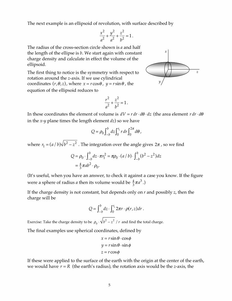
within a given volume. First we choose for the volume a tetrahedron as shown. The sides in the coordinate planes are 45° triangles of side a. The other side is the equilateral triangle shown, which is in the plane described by

x + y + z = a . We will assume the charge

density is a constant: !(x, y,z) = !0 . The total charge is then

!

0 times the volume of the tetrahedron.

The integrals will be done in the order x, y, z. We have

Q = !0 " dz0

a

# " dy0

a$z

# " dx0

a$y$z

#= !0 " dz

0

a

# " (a $ y $ z)dy0

a$z

#= !0 "

12

(a $ z)2 dz0

a

#=

16!0a3.

The tetrahedron has volume 1/6th that of a cube of side a.

r

dr

rdθ θ

x

y

z

5

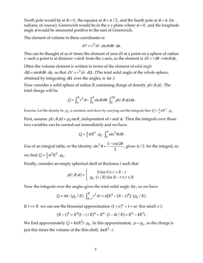
The next example is an ellipsoid of revolution, with surface described by

x2

a2+

y2

a2+

z2

b2= 1 .

The radius of the cross-section circle shown is a and half the length of the ellipse is b. We start again with constant charge density and calculate in effect the volume of the ellipsoid.

The first thing to notice is the symmetry with respect to rotation around the z-axis. If we use cylindrical coordinates (r ,! ,z) , where x = r cos! ,

y = r sin! , the

equation of the ellipsoid reduces to

r2

a2+

z2

b2= 1 .

In these coordinates the element of volume is dV = r dr !d" !dz (the area element

r dr !d"

in the x-y plane times the length element dz) so we have

Q = !

0dz

"b

b

# r dr0

r1# d$

0

2%# ,

where r1 = (a/b) b

2! z

2 . The integration over the angle gives 2! , so we find

Q = !0 " dz#b

b

$ "%r12= %!0 " (a/b) " (b2 # z2 )dz

#b

b

$=

43% ab2 " !0.

(It’s useful, when you have an answer, to check it against a case you know. If the figure were a sphere of radius a then its volume would be

4

3! a

3 .)

If the charge density is not constant, but depends only on r and possibly z, then the charge will be

Q = dz

!b

b

" # 2$r # %(r ,z)dr0

r1" .

Exercise: Take the charge density to be !

0" b

2# z

2/ r and find the total charge.

The final examples use spherical coordinates, defined by

x = r sin! "cos#

y = r sin! "sin#

z = r cos#

If these were applied to the surface of the earth with the origin at the center of the earth, we would have r = R (the earth’s radius), the rotation axis would be the z-axis, the

x

z

y

6

North pole would be at ! = 0 , the equator at ! = " /2 , and the South pole at ! = " (in radians, of course). Greenwich would be in the x-z plane where

! = 0 , and the longitude

angle ! would be measured positive to the east of Greenwich.

The element of volume in these coordinates is

dV = r

2dr !sin" d" !d# .

This can be thought of as dr times the element of area dS at a point on a sphere of radius r; such a point is at distance r sin! from the z-axis, so the element is

dS = r d! " r sin! d# .

Often the volume element is written in terms of the element of solid angle

d! = sin" d" #d$ , so that

dV = r

2dr !d" . (The total solid angle of the whole sphere,

obtained by integrating d! over the angles, is 4! .) Now consider a solid sphere of radius R containing charge of density !(r ," ,#) . The total charge will be

Q = r2 dr

0

R

! " sin# d#0

$! " %(r ,# ,&)d&

0

2$! .

Exercise: Let the density be !

0, a constant, and show by carrying out the integrals that

Q =

4

3!R

3" #

0.

First, assume !(r ," ,#) = !0 sin" , independent of r and ! . Then the integrals over those

two variables can be carried out immediately and we have

Q =

2

3!R3 " #

0" sin

2$ d$0

!% .

Use of an integral table, or the identity

sin2! =

1 " cos2!

2, gives ! /2 for the integral, so

we find Q =

1

3! 2R3 " #

0.

Finally, consider an empty spherical shell of thickness t such that

!(r ," ,#) =0 for 0 $ r < R % t

!0 & (r /R) for R % t $ r $ R

'()

*)

Now the integrals over the angles gives the total solid angle 4! , so we have

Q = 4! " (#0 /R) " r3 dr

R$t

R

% = ![R4 $ (R $ t)4] " (#0 /R) .

If t << R we can use the binomial approximation (1 + !)n" 1 + n! (for small ! ):

(R ! t)4= R

4(1 ! t/R)4" R

4# (1 ! 4t/R) = R

4! 4R

3t .

We find approximately Q ! 4"R2t # $

0. In this approximation,

! " !

0, so the charge is

just this times the volume of the thin shell, 4!R2" t .