Multiple Two-Sample T-Tests - Sample Size - · PDF fileMultiple Two-Sample T-Tests 615-2 ... When the two-sample T-test is run for a replicated microarray experiment, the result is

PASS Sample Size Software NCSS.com

615-1 © NCSS, LLC. All Rights Reserved.

Chapter 615

Multiple Two-Sample T-Tests Introduction This chapter describes how to estimate power and sample size (number of arrays) for 2 group (two-sample) high-throughput studies using the Multiple Two-Sample T-Tests procedure. False discovery rate and experiment-wise error rate control methods are available in this procedure. Values that can be varied in this procedure are power, false discovery rate and experiment-wise error rate, sample sizes (numbers of arrays) in each group, the minimum mean difference detected, the standard deviations in each group, and in the case of false discovery rate control, the number of genes with minimum mean difference.

Two-Sample Design In a two-sample design, two groups are compared, which we will call Treatment 1 and Treatment 2. Several experimental units are randomly assigned to each of the two treatment groups. In the microarray scenario, a single mRNA or cDNA sample is obtained from each experimental unit of both groups. Each sample is exposed to a single microarray, resulting in a single expression value for each gene for each unit of each treatment group. The goal is to determine for each gene whether there is evidence that the expression is different between the two groups.

Null and Alternative Hypotheses The two-sample null and alternative hypotheses are described here in terms of treatment groups: Treatment 1 and Treatment 2. These groups could equally be labeled Treatment A and Treatment B, Control and Treatment, etc. The two-sample null hypothesis for each gene is H0: µ1 = µ2, where µ1 is the true mean expression for that particular gene in the Treatment 1 environment, and µ2 is the true mean expression for that particular gene following Treatment 2. The alternative hypothesis may be any one of the following: Ha: µ1 < µ2, Ha: µ1 > µ2, or Ha: µ1 ≠ µ2. The choice of the alternative hypothesis depends upon the goals of the research. For example, if the goal of the experiment is only to determine which genes are up-regulated (increase in expression) over Treatment 1 when Treatment 2 is imposed, the alternative hypothesis would be Ha: µ1 < µ2. If the goal instead is to determine which genes are differentially expressed (up-regulated or down-regulated) when compared to the other treatment, the alternative hypothesis is Ha: µ1 ≠ µ2.

PASS Sample Size Software NCSS.com Multiple Two-Sample T-Tests


Assumptions The following assumptions are made when using the two-sample T-test or the Mann-Whitney U test. One of the reasons for the popularity of the T-test is its robustness in the face of assumption violation. However, if an assumption is not met even approximately, the significance levels and the power of the T-test are unknown. You should take the appropriate steps to check the assumptions before you make important decisions based on these tests.

Two-Sample T-Test Assumptions The assumptions of the two-sample T-test are:

1. The data are continuous (not discrete).

2. The data follow the normal probability distribution.

3. The variances of the two populations are equal. (If not, the Aspin-Welch Unequal-Variance test is used.)

4. The two samples are independent. There is no relationship between the individuals in one sample as compared to the other (as there is in the paired T-test).

5. Both samples are simple random samples from their respective populations. Each individual in the population has an equal probability of being selected in the sample.

Mann-Whitney U Test Assumptions The assumptions of the Mann-Whitney U test for difference in means are:

1. The variable of interest is continuous (not discrete). The measurement scale is at least ordinal.

2. The probability distributions of the two populations are identical, except for location. That is, the variances are equal.

3. The two samples are independent.

4. Both samples are simple random samples from their respective populations. Each individual in the population has an equal probability of being selected in the sample.

Technical Details

Multiple Testing Adjustment When the two-sample T-test is run for a replicated microarray experiment, the result is a list of P-values (Probability Levels) that reflect the evidence of difference in expression. When hundreds or thousands of genes are investigated at the same time, many ‘small’ P-values will occur by chance, due to the natural variability of the process. It is therefore requisite to make an appropriate adjustment to the P-value (Probability Level), such that the likelihood of a false conclusion is controlled.

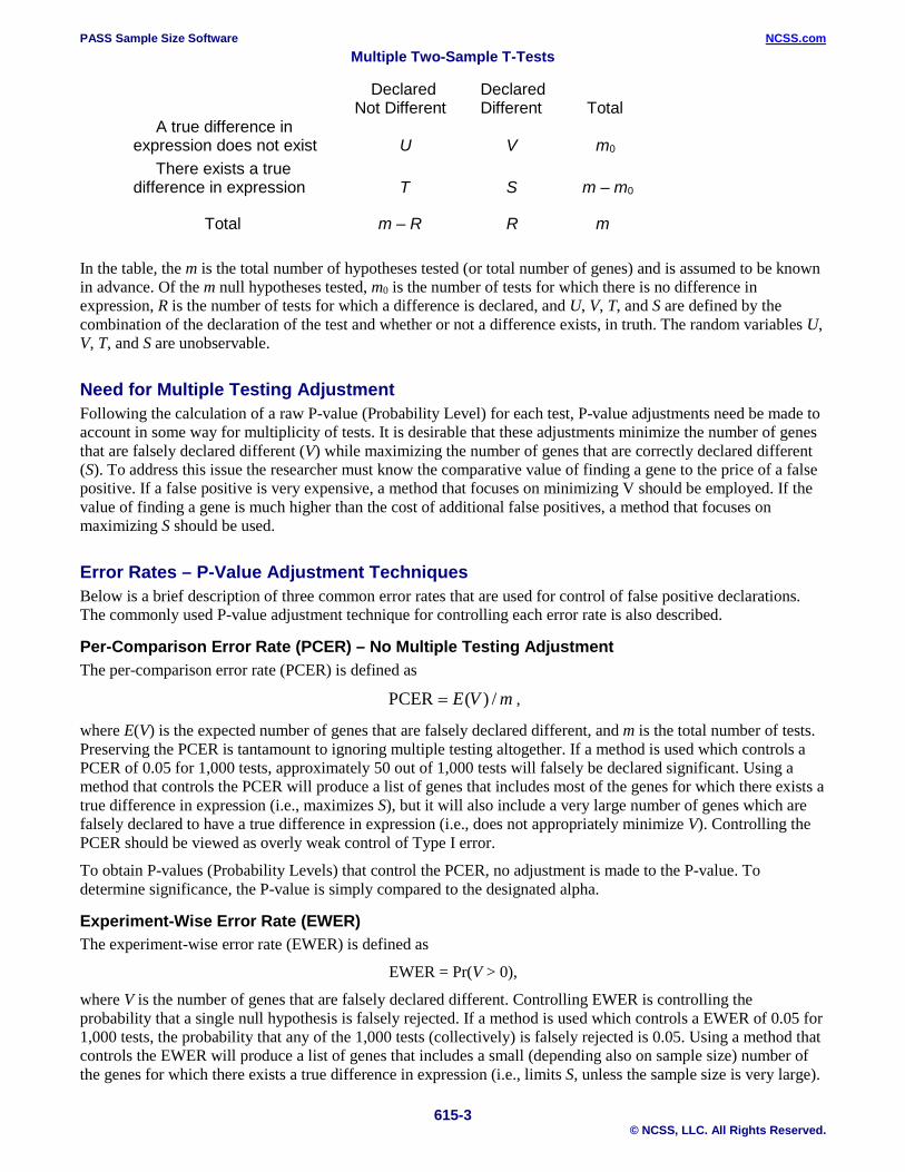
Benjamini and Hochberg’s (1995) False Discovery Rate Table The following table (adapted to the subject of microarray data) is found in Benjamini and Hochberg’s (1995) false discovery rate article. In the table, m is the total number of tests, m0 is the number of tests for which there is no difference in expression, R is the number of tests for which a difference is declared, and U, V, T, and S are defined by the combination of the declaration of the test and whether or not a difference exists, in truth.



Declared Declared Not Different Different Total

A true difference in expression does not exist U V m0

There exists a true difference in expression T S m – m0

Total m – R R m

In the table, the m is the total number of hypotheses tested (or total number of genes) and is assumed to be known in advance. Of the m null hypotheses tested, m0 is the number of tests for which there is no difference in expression, R is the number of tests for which a difference is declared, and U, V, T, and S are defined by the combination of the declaration of the test and whether or not a difference exists, in truth. The random variables U, V, T, and S are unobservable.

Need for Multiple Testing Adjustment Following the calculation of a raw P-value (Probability Level) for each test, P-value adjustments need be made to account in some way for multiplicity of tests. It is desirable that these adjustments minimize the number of genes that are falsely declared different (V) while maximizing the number of genes that are correctly declared different (S). To address this issue the researcher must know the comparative value of finding a gene to the price of a false positive. If a false positive is very expensive, a method that focuses on minimizing V should be employed. If the value of finding a gene is much higher than the cost of additional false positives, a method that focuses on maximizing S should be used.

Error Rates – P-Value Adjustment Techniques Below is a brief description of three common error rates that are used for control of false positive declarations. The commonly used P-value adjustment technique for controlling each error rate is also described.

Per-Comparison Error Rate (PCER) – No Multiple Testing Adjustment The per-comparison error rate (PCER) is defined as

PCER ( ) /E V m= ,

where E(V) is the expected number of genes that are falsely declared different, and m is the total number of tests. Preserving the PCER is tantamount to ignoring multiple testing altogether. If a method is used which controls a PCER of 0.05 for 1,000 tests, approximately 50 out of 1,000 tests will falsely be declared significant. Using a method that controls the PCER will produce a list of genes that includes most of the genes for which there exists a true difference in expression (i.e., maximizes S), but it will also include a very large number of genes which are falsely declared to have a true difference in expression (i.e., does not appropriately minimize V). Controlling the PCER should be viewed as overly weak control of Type I error.

To obtain P-values (Probability Levels) that control the PCER, no adjustment is made to the P-value. To determine significance, the P-value is simply compared to the designated alpha.

Experiment-Wise Error Rate (EWER) The experiment-wise error rate (EWER) is defined as

EWER = Pr(V > 0),

where V is the number of genes that are falsely declared different. Controlling EWER is controlling the probability that a single null hypothesis is falsely rejected. If a method is used which controls a EWER of 0.05 for 1,000 tests, the probability that any of the 1,000 tests (collectively) is falsely rejected is 0.05. Using a method that controls the EWER will produce a list of genes that includes a small (depending also on sample size) number of the genes for which there exists a true difference in expression (i.e., limits S, unless the sample size is very large).



However, the list of genes will include very few or no genes that are falsely declared to have a true difference in expression (i.e., stringently minimizes V). Controlling the EWER should be considered very strong control of Type I error.

Assuming the tests are independent, the well-known Bonferroni P-value adjustment produces adjusted P-values (Probability Levels) for which the EWER is controlled. The Bonferroni adjustment is applied to all m unadjusted P-values ( jp ) as

min( ,1)j jp mp= .

That is, each P-value (Probability Level) is multiplied by the number of tests, and if the result is greater than one, it is set to the maximum possible P-value of one.

False Discovery Rate (FDR) The false discovery rate (FDR) (Benjamini and Hochberg, 1995) is defined as

{ 0}FDR ( 1 ) ( | 0) Pr( 0)RV VE E R RR R>= = > > ,

where R is the number of genes that are declared significantly different, and V is the number of genes that are falsely declared different. Controlling FDR is controlling the expected proportion of falsely declared differences (false discoveries) to declared differences (true and false discoveries, together). If a method is used which controls a FDR of 0.05 for 1,000 tests, and 40 genes are declared different, it is expected that 40*0.05 = 2 of the 40 declarations are false declarations (false discoveries). Using a method that controls the FDR will produce a list of genes that includes an intermediate (depending also on sample size) number of genes for which there exists a true difference in expression (i.e., moderate to large S). However, the list of genes will include a small number of genes that are falsely declared to have a true difference in expression (i.e., moderately minimizes V). Controlling the FDR should be considered intermediate control of Type I error.

Assuming the tests are independent, the Benjamini and Hochberg P-value adjustment produces adjusted P-values (Probability Levels) for which the FDR is controlled. These adjusted P-values are found as

,...,min {min( ,1)}

i kr rk i m

mp pk=

= ,

where 1 2 mr r rp p p≤ ≤ ≤ are the observed ordered unadjusted P-values. The procedure is defined in Benjamini

and Hochberg (1995). The corresponding adjusted P-value definition given here is found in Dudoit, Shaffer, and Boldrick (2003).

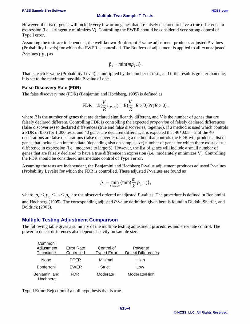
Multiple Testing Adjustment Comparison The following table gives a summary of the multiple testing adjustment procedures and error rate control. The power to detect differences also depends heavily on sample size.

Common Adjustment Error Rate Control of Power to Technique Controlled Type I Error Detect Differences

None PCER Minimal High

Bonferroni EWER Strict Low

Benjamini and FDR Moderate Moderate/High Hochberg

Type I Error: Rejection of a null hypothesis that is true.



Calculating Power Additional details of calculating power in the two-group scenario are found in the PASS chapter for Two Means.

There are four separate situations, each requiring different formulas. Let the means of the two populations be represented by µ1 and µ2 . The difference between these means will be represented by d. Let the standard deviations of the two populations be represented as σ1 and σ2 .

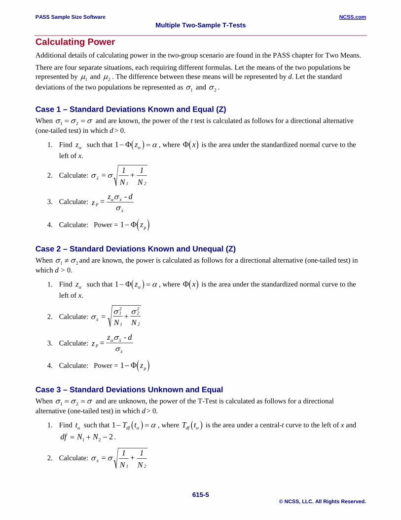
Case 1 – Standard Deviations Known and Equal (Z) When σ σ σ1 2= = and are known, the power of the t test is calculated as follows for a directional alternative (one-tailed test) in which d > 0.

1. Find zα such that ( )1− =Φ zα α , where ( )Φ x is the area under the standardized normal curve to the left of x.

2. Calculate: σ σx1 2

= 1N

+ 1N

3. Calculate: px

xz = z - dασ

σ

4. Calculate: Power = ( )1− Φ zp

Case 2 – Standard Deviations Known and Unequal (Z) When σ σ1 2≠ and are known, the power is calculated as follows for a directional alternative (one-tailed test) in which d > 0.

1. Find zα such that ( )1− =Φ zα α , where ( )Φ x is the area under the standardized normal curve to the left of x.

2. Calculate: σσ σ

x12

1

22

2=

N+

N

3. Calculate: px

xz =

z - dασσ

4. Calculate: Power = ( )1− Φ zp

Case 3 – Standard Deviations Unknown and Equal When σ σ σ1 2= = and are unknown, the power of the T-Test is calculated as follows for a directional alternative (one-tailed test) in which d > 0.

1. Find tα such that ( )1− =T tdf α α , where ( )T tdf α is the area under a central-t curve to the left of x and df N N= + −1 2 2 .

2. Calculate: σ σx1 2

= 1N

+ 1N



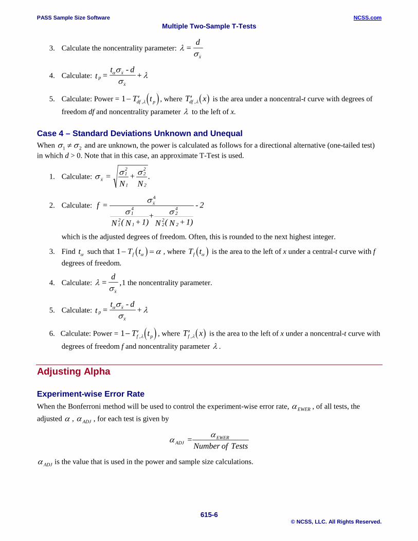
3. Calculate the noncentrality parameter: λσ

=d

x

4. Calculate: px

xt =

t - d+ασ

σλ

5. Calculate: Power = ( )1− ′T tdf p,λ , where ( )′T xdf ,λ is the area under a noncentral-t curve with degrees of

freedom df and noncentrality parameter λ to the left of x.

Case 4 – Standard Deviations Unknown and Unequal When σ σ1 2≠ and are unknown, the power is calculated as follows for a directional alternative (one-tailed test) in which d > 0. Note that in this case, an approximate T-Test is used.

1. Calculate: σ σ σx

12

1

22

2=

N+

N.

2. Calculate: f =

N ( N +1)+

N ( N +1)

- 2x

14

12

1

24

22

2

σσ σ

4

which is the adjusted degrees of freedom. Often, this is rounded to the next highest integer.

3. Find tα such that ( )1− =T tf α α , where ( )T tf α is the area to the left of x under a central-t curve with f degrees of freedom.

4. Calculate: λσ

=d

,x

1 the noncentrality parameter.

5. Calculate: px

xt =

t - d+ασ

σλ

6. Calculate: Power = ( )1− ′T tf p,λ , where ( )′T xf ,λ is the area to the left of x under a noncentral-t curve with

degrees of freedom f and noncentrality parameter λ .

Adjusting Alpha

Experiment-wise Error Rate When the Bonferroni method will be used to control the experiment-wise error rate, EWERα , of all tests, the adjusted α , ADJα , for each test is given by

Tests ofNumber = EWER

ADJαα

ADJα is the value that is used in the power and sample size calculations.



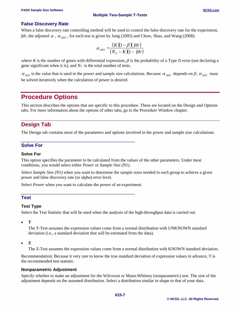
False Discovery Rate When a false discovery rate controlling method will be used to control the false discovery rate for the experiment, fdr, the adjusted α , ADJα , for each test is given by Jung (2005) and Chow, Shao, and Wang (2008):

( )( )( )( )( )fdrKN

fdrK=T

ADJ −−−

11 βα

where K is the number of genes with differential expression, β is the probability of a Type II error (not declaring a gene significant when it is), and NT is the total number of tests.

ADJα is the value that is used in the power and sample size calculations. Because ADJα depends on β, ADJα must be solved iteratively when the calculation of power is desired.

Procedure Options This section describes the options that are specific to this procedure. These are located on the Design and Options tabs. For more information about the options of other tabs, go to the Procedure Window chapter.

Design Tab The Design tab contains most of the parameters and options involved in the power and sample size calculations.

Solve For

Solve For This option specifies the parameter to be calculated from the values of the other parameters. Under most conditions, you would select either Power or Sample Size (N1).

Select Sample Size (N1) when you want to determine the sample sizes needed in each group to achieve a given power and false discovery rate (or alpha) error level.

Select Power when you want to calculate the power of an experiment.

Test

Test Type Select the Test Statistic that will be used when the analysis of the high-throughput data is carried out.

• T The T-Test assumes the expression values come from a normal distribution with UNKNOWN standard deviation (i.e., a standard deviation that will be estimated from the data).

• Z The Z-Test assumes the expression values come from a normal distribution with KNOWN standard deviation.

Recommendation: Because it very rare to know the true standard deviation of expression values in advance, T is the recommended test statistic.

Nonparametric Adjustment Specify whether to make an adjustment for the Wilcoxon or Mann-Whitney (nonparametric) test. The size of the adjustment depends on the assumed distribution. Select a distribution similar in shape to that of your data.



Alternative Specify whether the hypothesis test for each gene is one-sided (directional) or two-sided (non-directional).

Recommendation: In most two-group experiments, differential expression in either direction (up-regulation or down-regulation) is of interest. Such experiments should have the Two-Sided alternative hypothesis.

For experiments for determining only whether expression has increased (or only decreased), a One-Sided alternative hypothesis is recommended. Often regulations dictate that the FDR or EWER level be divided by 2 for One-Sided alternative tests.

Error Rates

Power for each Test Power is the probability of rejecting each null hypothesis when it is false. Power is equal to 1-Beta.

The POWER for each gene represents that probability of detecting differential expression when it exists.

RANGE: The valid range is from 0 to 1.

RECOMMENDED: Popular values for power are 0.8 and 0.9.

NOTES: You can enter a range of values such as .70 .80 .90 or .70 to .95 by .05.

False Discovery (Alpha) Method A type I error is declaring a gene to be differentially expressed when it is not. The two most common methods for controlling type I error in microarray expression studies are false discovery rate (FDR) control and Experiment-wise Error Rate (EWER) control.

• FDR Controlling the false discovery rate (FDR) controls the PROPORTION of genes that are falsely declared differentially expressed. For example, suppose that an FDR of 0.05 is used for 10000 tests (on 10000 genes). If differential expression is declared for 100 of the 10000 genes, 5 of the 100 genes are expected to be false discoveries.

• EWER Controlling the experiment-wise error rate (EWER) controls the PROBABILITY of ANY false declarations of differential expression, across all tests. For example, suppose that an EWER of 0.05 is used for 10000 tests (on 10000 genes). If differential expression is declared for 100 of the 10000 genes, the probability that even one of the 100 declarations is false is 0.05.

Recommendation: For exploratory studies where a list of candidate genes for further study is the goal, FDR is the recommended Type I error control method, because of its higher power.

For confirmatory studies where final determination of differential expression is the goal, EWER is the recommended Type I error control method, because of its strict control of false discoveries.

FDR or EWER Value Specify the value for the False Discovery (Alpha) Method selected above.

RANGE: These levels are bounded by 0 and 1. Commonly, the chosen level is between 0.001 and 0.250

RECOMMENDED: FDR or EWER is often set to 0.05 for two-sided tests and to 0.025 for one-sided tests.

NOTE: You can enter a list of values such as .05 .10 .15 or .05 to .15 by .01.



Sample Size (When Solving for Sample Size)

Group Allocation Select the option that describes the constraints on N1 or N2 or both.

The options are

• Equal (N1 = N2) This selection is used when you wish to have equal sample sizes in each group. Since you are solving for both sample sizes at once, no additional sample size parameters need to be entered.

• Enter N1, solve for N2 Select this option when you wish to fix N1 at some value (or values), and then solve only for N2. Please note that for some values of N1, there may not be a value of N2 that is large enough to obtain the desired power.

• Enter N2, solve for N1 Select this option when you wish to fix N2 at some value (or values), and then solve only for N1. Please note that for some values of N2, there may not be a value of N1 that is large enough to obtain the desired power.

• Enter R = N2/N1, solve for N1 and N2 For this choice, you set a value for the ratio of N2 to N1, and then PASS determines the needed N1 and N2, with this ratio, to obtain the desired power. An equivalent representation of the ratio, R, is

N2 = R * N1.

• Enter percentage in Group 1, solve for N1 and N2 For this choice, you set a value for the percentage of the total sample size that is in Group 1, and then PASS determines the needed N1 and N2 with this percentage to obtain the desired power.

N1 (Number of Arrays, Group 1) This option is displayed if Group Allocation = “Enter N1, solve for N2”

N1 is the number of items or individuals sampled from the Group 1 population.

N1 must be ≥ 2. You can enter a single value or a series of values.

N2 (Number of Arrays, Group 2) This option is displayed if Group Allocation = “Enter N2, solve for N1”



R (Group Sample Size Ratio) This option is displayed only if Group Allocation = “Enter R = N2/N1, solve for N1 and N2.”

R is the ratio of N2 to N1. That is,

R = N2 / N1.

Use this value to fix the ratio of N2 to N1 while solving for N1 and N2. Only sample size combinations with this ratio are considered.

N2 is related to N1 by the formula:

N2 = [R × N1],

where the value [Y] is the next integer ≥ Y.



For example, setting R = 2.0 results in a Group 2 sample size that is double the sample size in Group 1 (e.g., N1 = 10 and N2 = 20, or N1 = 50 and N2 = 100).

R must be greater than 0. If R < 1, then N2 will be less than N1; if R > 1, then N2 will be greater than N1. You can enter a single or a series of values.

Percent in Group 1 This option is displayed only if Group Allocation = “Enter percentage in Group 1, solve for N1 and N2.”

Use this value to fix the percentage of the total sample size allocated to Group 1 while solving for N1 and N2. Only sample size combinations with this Group 1 percentage are considered. Small variations from the specified percentage may occur due to the discrete nature of sample sizes.

The Percent in Group 1 must be greater than 0 and less than 100. You can enter a single or a series of values.

Sample Size (When Not Solving for Sample Size)

Group Allocation Select the option that describes how individuals in the study will be allocated to Group 1 and to Group 2.

The options are

• Equal (N1 = N2) This selection is used when you wish to have equal sample sizes in each group. A single per group sample size will be entered.

• Enter N1 and N2 individually This choice permits you to enter different values for N1 and N2.

• Enter N1 and R, where N2 = R * N1 Choose this option to specify a value (or values) for N1, and obtain N2 as a ratio (multiple) of N1.

• Enter total sample size and percentage in Group 1 Choose this option to specify a value (or values) for the total sample size (N), obtain N1 as a percentage of N, and then N2 as N - N1.

Sample Size Per Group This option is displayed only if Group Allocation = “Equal (N1 = N2).”

The Sample Size Per Group is the number of items or individuals sampled from each of the Group 1 and Group 2 populations. Since the sample sizes are the same in each group, this value is the value for N1, and also the value for N2.

The Sample Size Per Group must be ≥ 2. You can enter a single value or a series of values.

N1 (Number of Arrays, Group 1) This option is displayed if Group Allocation = “Enter N1 and N2 individually” or “Enter N1 and R, where N2 = R * N1.”





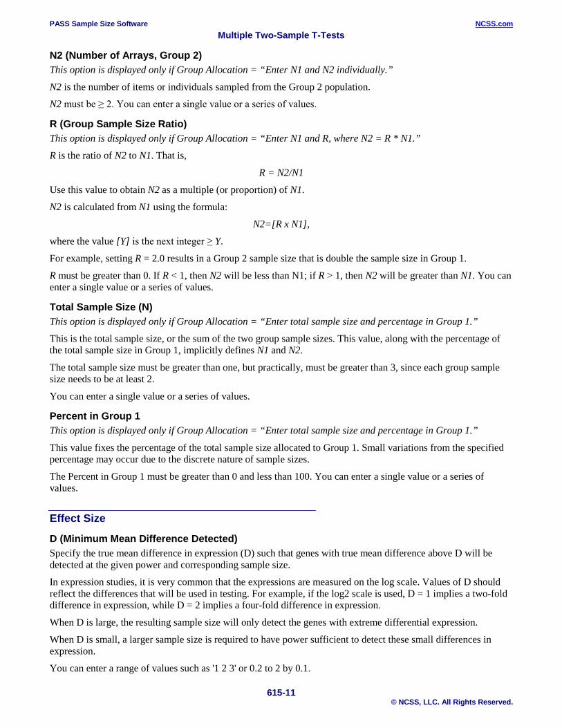
N2 (Number of Arrays, Group 2) This option is displayed only if Group Allocation = “Enter N1 and N2 individually.”



R (Group Sample Size Ratio) This option is displayed only if Group Allocation = “Enter N1 and R, where N2 = R * N1.”

R is the ratio of N2 to N1. That is,

R = N2/N1

Use this value to obtain N2 as a multiple (or proportion) of N1.

N2 is calculated from N1 using the formula:

N2=[R x N1],

where the value [Y] is the next integer ≥ Y.

For example, setting R = 2.0 results in a Group 2 sample size that is double the sample size in Group 1.

R must be greater than 0. If R < 1, then N2 will be less than N1; if R > 1, then N2 will be greater than N1. You can enter a single value or a series of values.

Total Sample Size (N) This option is displayed only if Group Allocation = “Enter total sample size and percentage in Group 1.”

This is the total sample size, or the sum of the two group sample sizes. This value, along with the percentage of the total sample size in Group 1, implicitly defines N1 and N2.

The total sample size must be greater than one, but practically, must be greater than 3, since each group sample size needs to be at least 2.

You can enter a single value or a series of values.

Percent in Group 1 This option is displayed only if Group Allocation = “Enter total sample size and percentage in Group 1.”

This value fixes the percentage of the total sample size allocated to Group 1. Small variations from the specified percentage may occur due to the discrete nature of sample sizes.

The Percent in Group 1 must be greater than 0 and less than 100. You can enter a single value or a series of values.

Effect Size

D (Minimum Mean Difference Detected) Specify the true mean difference in expression (D) such that genes with true mean difference above D will be detected at the given power and corresponding sample size.

In expression studies, it is very common that the expressions are measured on the log scale. Values of D should reflect the differences that will be used in testing. For example, if the log2 scale is used, D = 1 implies a two-fold difference in expression, while D = 2 implies a four-fold difference in expression.

When D is large, the resulting sample size will only detect the genes with extreme differential expression.

When D is small, a larger sample size is required to have power sufficient to detect these small differences in expression.

You can enter a range of values such as '1 2 3' or 0.2 to 2 by 0.1.



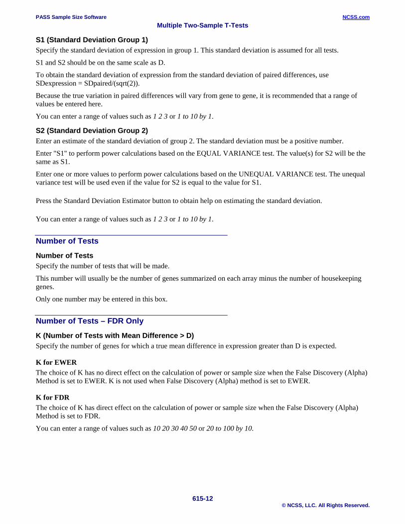
S1 (Standard Deviation Group 1) Specify the standard deviation of expression in group 1. This standard deviation is assumed for all tests.

S1 and S2 should be on the same scale as D.

To obtain the standard deviation of expression from the standard deviation of paired differences, use SDexpression = SDpaired/(sqrt(2)).

Because the true variation in paired differences will vary from gene to gene, it is recommended that a range of values be entered here.

You can enter a range of values such as 1 2 3 or 1 to 10 by 1.

S2 (Standard Deviation Group 2) Enter an estimate of the standard deviation of group 2. The standard deviation must be a positive number.

Enter "S1" to perform power calculations based on the EQUAL VARIANCE test. The value(s) for S2 will be the same as S1.

Enter one or more values to perform power calculations based on the UNEQUAL VARIANCE test. The unequal variance test will be used even if the value for S2 is equal to the value for S1. Press the Standard Deviation Estimator button to obtain help on estimating the standard deviation. You can enter a range of values such as 1 2 3 or 1 to 10 by 1.

Number of Tests

Number of Tests Specify the number of tests that will be made.

This number will usually be the number of genes summarized on each array minus the number of housekeeping genes.

Only one number may be entered in this box.

Number of Tests – FDR Only

K (Number of Tests with Mean Difference > D) Specify the number of genes for which a true mean difference in expression greater than D is expected.

K for EWER The choice of K has no direct effect on the calculation of power or sample size when the False Discovery (Alpha) Method is set to EWER. K is not used when False Discovery (Alpha) method is set to EWER.

K for FDR The choice of K has direct effect on the calculation of power or sample size when the False Discovery (Alpha) Method is set to FDR.

You can enter a range of values such as 10 20 30 40 50 or 20 to 100 by 10.



Options Tab The Options tab contains convergence options that are rarely changed.

Convergence Options

FDR Power Convergence When FDR is selected for False Discovery (Alpha) Method, and Find (Solve For) is set to Power, the corresponding search algorithm will converge when the search criteria is below this value.

This value will rarely be changed from the default value.

RECOMMENDED: 0.0000000001



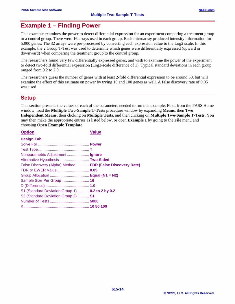
Example 1 – Finding Power This example examines the power to detect differential expression for an experiment comparing a treatment group to a control group. There were 16 arrays used in each group. Each microarray produced intensity information for 5,000 genes. The 32 arrays were pre-processed by converting each expression value to the Log2 scale. In this example, the 2 Group T-Test was used to determine which genes were differentially expressed (upward or downward) when comparing the treatment group to the control group.

The researchers found very few differentially expressed genes, and wish to examine the power of the experiment to detect two-fold differential expression (Log2-scale difference of 1). Typical standard deviations in each group ranged from 0.2 to 2.0.

The researchers guess the number of genes with at least 2-fold differential expression to be around 50, but will examine the effect of this estimate on power by trying 10 and 100 genes as well. A false discovery rate of 0.05 was used.

Setup This section presents the values of each of the parameters needed to run this example. First, from the PASS Home window, load the Multiple Two-Sample T-Tests procedure window by expanding Means, then Two Independent Means, then clicking on Multiple Tests, and then clicking on Multiple Two-Sample T-Tests. You may then make the appropriate entries as listed below, or open Example 1 by going to the File menu and choosing Open Example Template.

Option Value Design Tab Solve For ................................................ Power Test Type ................................................ T Nonparametric Adjustment ..................... Ignore Alternative Hypothesis ............................ Two-Sided False Discovery (Alpha) Method ............ FDR (False Discovery Rate) FDR or EWER Value .............................. 0.05 Group Allocation ..................................... Equal (N1 = N2) Sample Size Per Group .......................... 16 D (Difference) ......................................... 1.0 S1 (Standard Deviation Group 1) ........... 0.2 to 2 by 0.2 S2 (Standard Deviation Group 2) ........... S1 Number of Tests ..................................... 5000 K.............................................................. 10 50 100



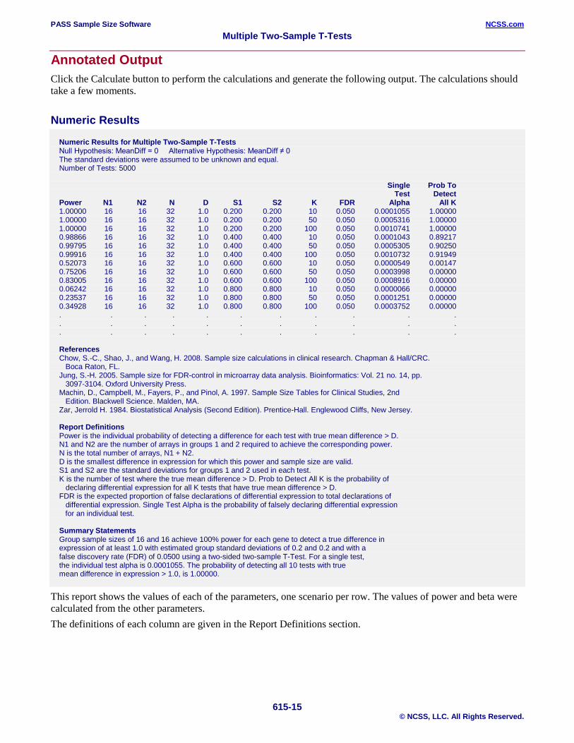
Annotated Output Click the Calculate button to perform the calculations and generate the following output. The calculations should take a few moments.

Numeric Results Numeric Results for Multiple Two-Sample T-Tests Null Hypothesis: MeanDiff = 0 Alternative Hypothesis: MeanDiff ≠ 0 The standard deviations were assumed to be unknown and equal. Number of Tests: 5000 Single Prob To Test Detect Power N1 N2 N D S1 S2 K FDR Alpha All K 1.00000 16 16 32 1.0 0.200 0.200 10 0.050 0.0001055 1.00000 1.00000 16 16 32 1.0 0.200 0.200 50 0.050 0.0005316 1.00000 1.00000 16 16 32 1.0 0.200 0.200 100 0.050 0.0010741 1.00000 0.98866 16 16 32 1.0 0.400 0.400 10 0.050 0.0001043 0.89217 0.99795 16 16 32 1.0 0.400 0.400 50 0.050 0.0005305 0.90250 0.99916 16 16 32 1.0 0.400 0.400 100 0.050 0.0010732 0.91949 0.52073 16 16 32 1.0 0.600 0.600 10 0.050 0.0000549 0.00147 0.75206 16 16 32 1.0 0.600 0.600 50 0.050 0.0003998 0.00000 0.83005 16 16 32 1.0 0.600 0.600 100 0.050 0.0008916 0.00000 0.06242 16 16 32 1.0 0.800 0.800 10 0.050 0.0000066 0.00000 0.23537 16 16 32 1.0 0.800 0.800 50 0.050 0.0001251 0.00000 0.34928 16 16 32 1.0 0.800 0.800 100 0.050 0.0003752 0.00000 . . . . . . . . . . . . . . . . . . . . . . . . . . . . . . . . . References Chow, S.-C., Shao, J., and Wang, H. 2008. Sample size calculations in clinical research. Chapman & Hall/CRC. Boca Raton, FL. Jung, S.-H. 2005. Sample size for FDR-control in microarray data analysis. Bioinformatics: Vol. 21 no. 14, pp. 3097-3104. Oxford University Press. Machin, D., Campbell, M., Fayers, P., and Pinol, A. 1997. Sample Size Tables for Clinical Studies, 2nd Edition. Blackwell Science. Malden, MA. Zar, Jerrold H. 1984. Biostatistical Analysis (Second Edition). Prentice-Hall. Englewood Cliffs, New Jersey. Report Definitions Power is the individual probability of detecting a difference for each test with true mean difference > D. N1 and N2 are the number of arrays in groups 1 and 2 required to achieve the corresponding power. N is the total number of arrays, N1 + N2. D is the smallest difference in expression for which this power and sample size are valid. S1 and S2 are the standard deviations for groups 1 and 2 used in each test. K is the number of test where the true mean difference > D. Prob to Detect All K is the probability of declaring differential expression for all K tests that have true mean difference > D. FDR is the expected proportion of false declarations of differential expression to total declarations of differential expression. Single Test Alpha is the probability of falsely declaring differential expression for an individual test. Summary Statements Group sample sizes of 16 and 16 achieve 100% power for each gene to detect a true difference in expression of at least 1.0 with estimated group standard deviations of 0.2 and 0.2 and with a false discovery rate (FDR) of 0.0500 using a two-sided two-sample T-Test. For a single test, the individual test alpha is 0.0001055. The probability of detecting all 10 tests with true mean difference in expression > 1.0, is 1.00000.

This report shows the values of each of the parameters, one scenario per row. The values of power and beta were calculated from the other parameters. The definitions of each column are given in the Report Definitions section.



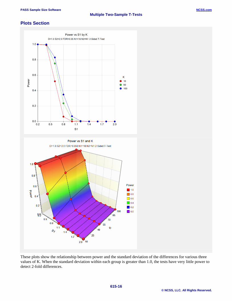
Plots Section

These plots show the relationship between power and the standard deviation of the differences for various three values of K. When the standard deviation within each group is greater than 1.0, the tests have very little power to detect 2-fold differences.



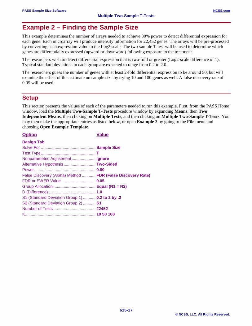
Example 2 – Finding the Sample Size This example determines the number of arrays needed to achieve 80% power to detect differential expression for each gene. Each microarray will produce intensity information for 22,452 genes. The arrays will be pre-processed by converting each expression value to the Log2 scale. The two-sample T-test will be used to determine which genes are differentially expressed (upward or downward) following exposure to the treatment.

The researchers wish to detect differential expression that is two-fold or greater (Log2-scale difference of 1). Typical standard deviations in each group are expected to range from 0.2 to 2.0.

The researchers guess the number of genes with at least 2-fold differential expression to be around 50, but will examine the effect of this estimate on sample size by trying 10 and 100 genes as well. A false discovery rate of 0.05 will be used.


Option Value Design Tab Solve For ................................................ Sample Size Test Type ................................................ T Nonparametric Adjustment ..................... Ignore Alternative Hypothesis ............................ Two-Sided Power ...................................................... 0.80 False Discovery (Alpha) Method ............ FDR (False Discovery Rate) FDR or EWER Value .............................. 0.05 Group Allocation ..................................... Equal (N1 = N2) D (Difference) ......................................... 1.0 S1 (Standard Deviation Group 1) ........... 0.2 to 2 by .2 S2 (Standard Deviation Group 2) ........... S1 Number of Tests ..................................... 22452 K.............................................................. 10 50 100



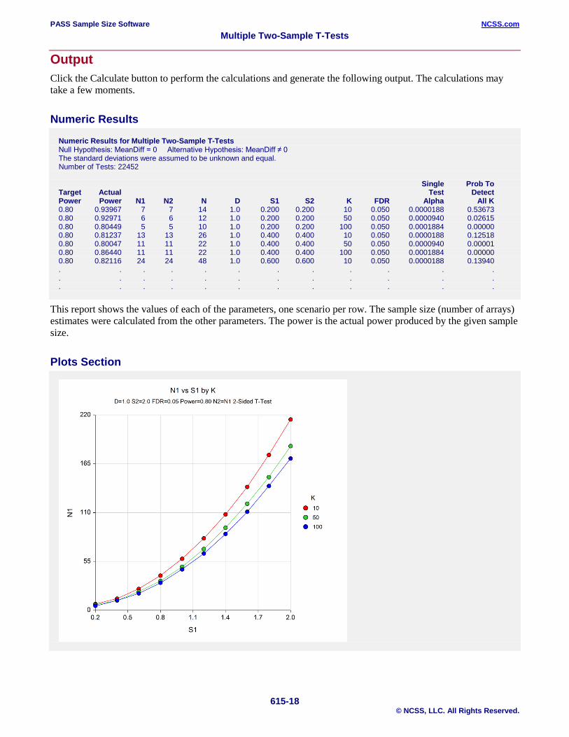
Output Click the Calculate button to perform the calculations and generate the following output. The calculations may take a few moments.

Numeric Results Numeric Results for Multiple Two-Sample T-Tests Null Hypothesis: MeanDiff = 0 Alternative Hypothesis: MeanDiff ≠ 0 The standard deviations were assumed to be unknown and equal. Number of Tests: 22452 Single Prob To Target Actual Test Detect Power Power N1 N2 N D S1 S2 K FDR Alpha All K 0.80 0.93967 7 7 14 1.0 0.200 0.200 10 0.050 0.0000188 0.53673 0.80 0.92971 6 6 12 1.0 0.200 0.200 50 0.050 0.0000940 0.02615 0.80 0.80449 5 5 10 1.0 0.200 0.200 100 0.050 0.0001884 0.00000 0.80 0.81237 13 13 26 1.0 0.400 0.400 10 0.050 0.0000188 0.12518 0.80 0.80047 11 11 22 1.0 0.400 0.400 50 0.050 0.0000940 0.00001 0.80 0.86440 11 11 22 1.0 0.400 0.400 100 0.050 0.0001884 0.00000 0.80 0.82116 24 24 48 1.0 0.600 0.600 10 0.050 0.0000188 0.13940 . . . . . . . . . . . . . . . . . . . . . . . . . . . . . . . . . . . .

This report shows the values of each of the parameters, one scenario per row. The sample size (number of arrays) estimates were calculated from the other parameters. The power is the actual power produced by the given sample size.

Plots Section



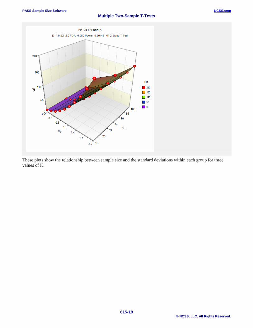
These plots show the relationship between sample size and the standard deviations within each group for three values of K.



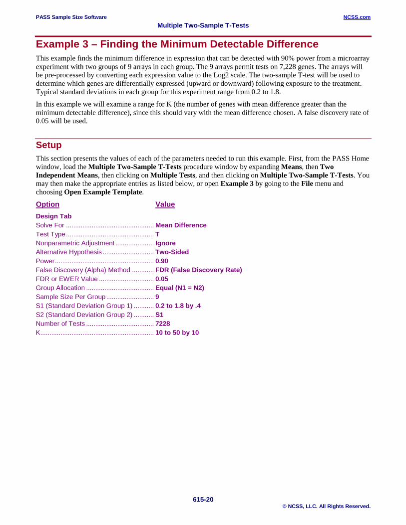
Example 3 – Finding the Minimum Detectable Difference This example finds the minimum difference in expression that can be detected with 90% power from a microarray experiment with two groups of 9 arrays in each group. The 9 arrays permit tests on 7,228 genes. The arrays will be pre-processed by converting each expression value to the Log2 scale. The two-sample T-test will be used to determine which genes are differentially expressed (upward or downward) following exposure to the treatment. Typical standard deviations in each group for this experiment range from 0.2 to 1.8.

In this example we will examine a range for K (the number of genes with mean difference greater than the minimum detectable difference), since this should vary with the mean difference chosen. A false discovery rate of 0.05 will be used.


Option Value Design Tab Solve For ................................................ Mean Difference Test Type ................................................ T Nonparametric Adjustment ..................... Ignore Alternative Hypothesis ............................ Two-Sided Power ...................................................... 0.90 False Discovery (Alpha) Method ............ FDR (False Discovery Rate) FDR or EWER Value .............................. 0.05 Group Allocation ..................................... Equal (N1 = N2) Sample Size Per Group .......................... 9 S1 (Standard Deviation Group 1) ........... 0.2 to 1.8 by .4 S2 (Standard Deviation Group 2) ........... S1 Number of Tests ..................................... 7228 K.............................................................. 10 to 50 by 10



Output Click the Calculate button to perform the calculations and generate the following output. The calculations may take a few moments.

Numeric Results Numeric Results for Multiple Two-Sample T-Tests Null Hypothesis: MeanDiff = 0 Alternative Hypothesis: MeanDiff ≠ 0 The standard deviations were assumed to be unknown and equal. Number of Tests: 7228 Single Prob To Test Detect Power N1 N2 N D S1 S2 K FDR Alpha All K 0.90000 9 9 18 0.6626 0.20 0.20 10 0.050 0.0000656 0.34868 0.90000 9 9 18 0.6253 0.20 0.20 20 0.050 0.0001314 0.12158 0.90000 9 9 18 0.6038 0.20 0.20 30 0.050 0.0001974 0.04239 0.90000 9 9 18 0.5888 0.20 0.20 40 0.050 0.0002636 0.01478 0.90000 9 9 18 0.5772 0.20 0.20 50 0.050 0.0003300 0.00515 0.90000 9 9 18 1.9879 0.60 0.60 10 0.050 0.0000656 0.34868 0.90000 9 9 18 1.8759 0.60 0.60 20 0.050 0.0001314 0.12158 0.90000 9 9 18 1.8115 0.60 0.60 30 0.050 0.0001974 0.04239 0.90000 9 9 18 1.7663 0.60 0.60 40 0.050 0.0002636 0.01478 0.90000 9 9 18 1.7315 0.60 0.60 50 0.050 0.0003300 0.00515 0.90000 9 9 18 3.3132 1.00 1.00 10 0.050 0.0000656 0.34868 0.90000 9 9 18 3.1265 1.00 1.00 20 0.050 0.0001314 0.12158 0.90000 9 9 18 3.0192 1.00 1.00 30 0.050 0.0001974 0.04239 . . . . . . . . . . . . . . . . . . . . . . . . . . . . . . . . .

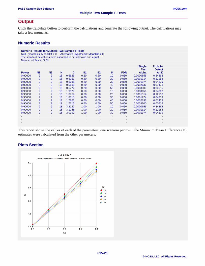
This report shows the values of each of the parameters, one scenario per row. The Minimum Mean Difference (D) estimates were calculated from the other parameters.

Plots Section



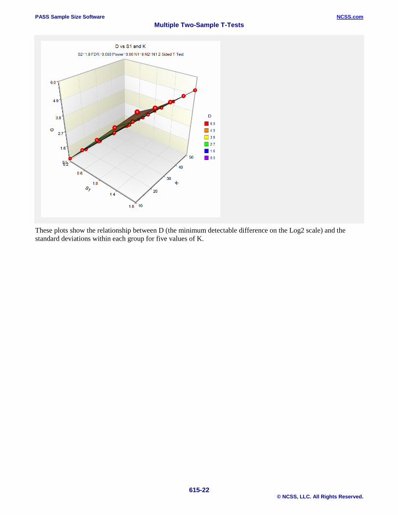
These plots show the relationship between D (the minimum detectable difference on the Log2 scale) and the standard deviations within each group for five values of K.



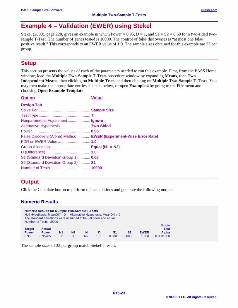
Example 4 – Validation (EWER) using Stekel Stekel (2003), page 228, gives an example in which Power = 0.95, D = 1, and S1 = S2 = 0.68 for a two-sided two-sample T-Test. The number of genes tested is 10000. The control of false discoveries is “at most one false positive result.” This corresponds to an EWER value of 1.0. The sample sizes obtained for this example are 33 per group.


Option Value Design Tab Solve For ................................................ Sample Size Test Type ................................................ T Nonparametric Adjustment ..................... Ignore Alternative Hypothesis ............................ Two-Sided Power ...................................................... 0.95 False Discovery (Alpha) Method ............ EWER (Experiment-Wise Error Rate) FDR or EWER Value .............................. 1.0 Group Allocation ..................................... Equal (N1 = N2) D (Difference) ......................................... 1.0 S1 (Standard Deviation Group 1) ........... 0.68 S2 (Standard Deviation Group 2) ........... S1 Number of Tests ..................................... 10000

Output Click the Calculate button to perform the calculations and generate the following output.

Numeric Results Numeric Results for Multiple Two-Sample T-Tests Null Hypothesis: MeanDiff = 0 Alternative Hypothesis: MeanDiff ≠ 0 The standard deviations were assumed to be unknown and equal. Number of Tests: 10000 Single Target Actual Test Power Power N1 N2 N D S1 S2 EWER Alpha 0.95 0.95785 33 33 66 1.0 0.680 0.680 1.000 0.0001000

The sample sizes of 33 per group match Stekel’s result.



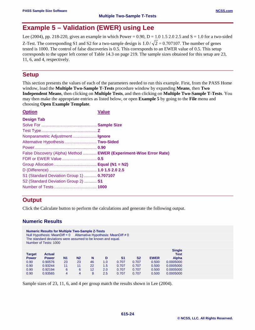
Example 5 – Validation (EWER) using Lee Lee (2004), pp. 218-220, gives an example in which Power = 0.90, D = 1.0 1.5 2.0 2.5 and S = 1.0 for a two-sided Z-Test. The corresponding S1 and S2 for a two-sample design is 2/0.1 = 0.707107. The number of genes tested is 1000. The control of false discoveries is 0.5. This corresponds to an EWER value of 0.5. This setup corresponds to the upper left corner of Table 14.3 on page 219. The sample sizes obtained for this setup are 23, 11, 6, and 4, respectively.


Option Value Design Tab Solve For ................................................ Sample Size Test Type ................................................ Z Nonparametric Adjustment ..................... Ignore Alternative Hypothesis ............................ Two-Sided Power ...................................................... 0.90 False Discovery (Alpha) Method ............ EWER (Experiment-Wise Error Rate) FDR or EWER Value .............................. 0.5 Group Allocation ..................................... Equal (N1 = N2) D (Difference) ......................................... 1.0 1.5 2.0 2.5 S1 (Standard Deviation Group 1) ........... 0.707107 S2 (Standard Deviation Group 2) ........... S1 Number of Tests ..................................... 1000


Numeric Results Numeric Results for Multiple Two-Sample Z-Tests Null Hypothesis: MeanDiff = 0 Alternative Hypothesis: MeanDiff ≠ 0 The standard deviations were assumed to be known and equal. Number of Tests: 1000 Single Target Actual Test Power Power N1 N2 N D S1 S2 EWER Alpha 0.90 0.90576 23 23 46 1.0 0.707 0.707 0.500 0.0005000 0.90 0.93244 11 11 22 1.5 0.707 0.707 0.500 0.0005000 0.90 0.92194 6 6 12 2.0 0.707 0.707 0.500 0.0005000 0.90 0.93565 4 4 8 2.5 0.707 0.707 0.500 0.0005000

Sample sizes of 23, 11, 6, and 4 per group match the results shown in Lee (2004).



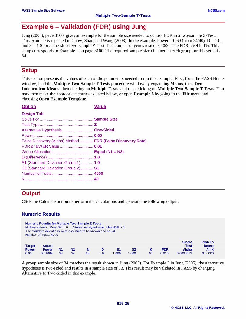
Example 6 – Validation (FDR) using Jung Jung (2005), page 3100, gives an example for the sample size needed to control FDR in a two-sample Z-Test. This example is repeated in Chow, Shao, and Wang (2008). In the example, Power = 0.60 (from 24/40), D = 1.0, and S = 1.0 for a one-sided two-sample Z-Test. The number of genes tested is 4000. The FDR level is 1%. This setup corresponds to Example 1 on page 3100. The required sample size obtained in each group for this setup is 34.


Option Value Design Tab Solve For ................................................ Sample Size Test Type ................................................ Z Alternative Hypothesis ............................ One-Sided Power ...................................................... 0.60 False Discovery (Alpha) Method ............ FDR (False Discovery Rate) FDR or EWER Value .............................. 0.01 Group Allocation ..................................... Equal (N1 = N2) D (Difference) ......................................... 1.0 S1 (Standard Deviation Group 1) ........... 1.0 S2 (Standard Deviation Group 2) ........... S1 Number of Tests ..................................... 4000 K.............................................................. 40


Numeric Results Numeric Results for Multiple Two-Sample Z-Tests Null Hypothesis: MeanDiff = 0 Alternative Hypothesis: MeanDiff > 0 The standard deviations were assumed to be known and equal. Number of Tests: 4000 Single Prob To Target Actual Test Detect Power Power N1 N2 N D S1 S2 K FDR Alpha All K 0.60 0.61099 34 34 68 1.0 1.000 1.000 40 0.010 0.0000612 0.00000

A group sample size of 34 matches the result shown in Jung (2005). For Example 3 in Jung (2005), the alternative hypothesis is two-sided and results in a sample size of 73. This result may be validated in PASS by changing Alternative to Two-Sided in this example.

Documents

Multiple Two-Sample T-Tests - Sample Size - · PDF fileMultiple Two-Sample T-Tests 615-2 ... When the two-sample T-test is run for a replicated microarray experiment, the result is