Hypothesis tests II. Two sample t-test, statistical errors.

1

2

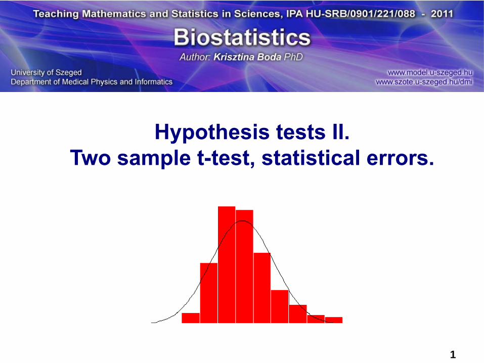
Motivating exampleTwo lecturers argue about the mean age of the first year medical students. Is the mean age for boys and girls the same or not?

Lecturer#1 claims that the mean age boys and girls is the same.Lecturer#2 does not agree. Who is right?

Statistically speaking: there are two populations:the set of ALL first year boy medical students (anywhere, any time) the set of ALL first year girl medical students (anywhere, any time)

Lecturer#1 claims that the population means are equal: μboys= μgirls. Lecturer#2 claims that the population means are not equal:μboyys ≠ μgirls.

3

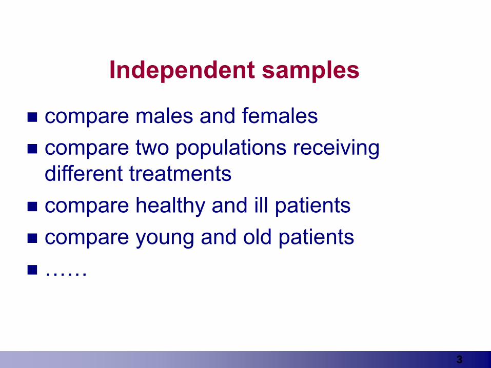
Independent samples

compare males and females compare two populations receiving different treatments compare healthy and ill patientscompare young and old patients……

4

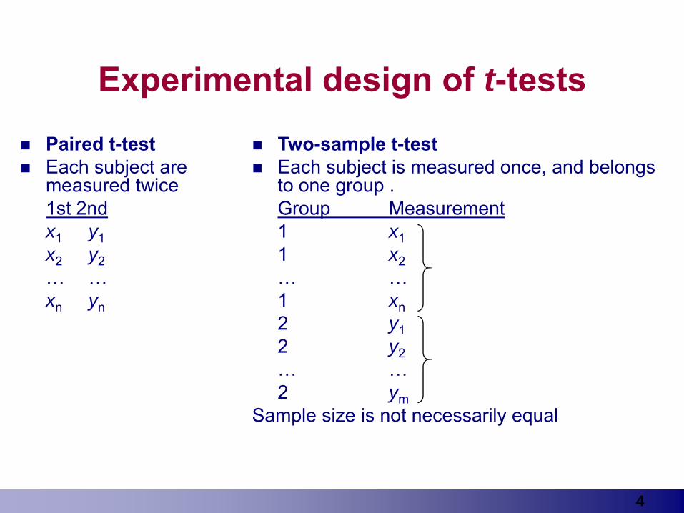
Experimental design of t-testsPaired t-testEach subject are measured twice1st 2ndx1 y1x2 y2… …xn yn

Two-sample t-testEach subject is measured once, and belongs to one group .Group Measurement1 x11 x2… …1 xn2 y12 y2… …2 ym

Sample size is not necessarily equal

5

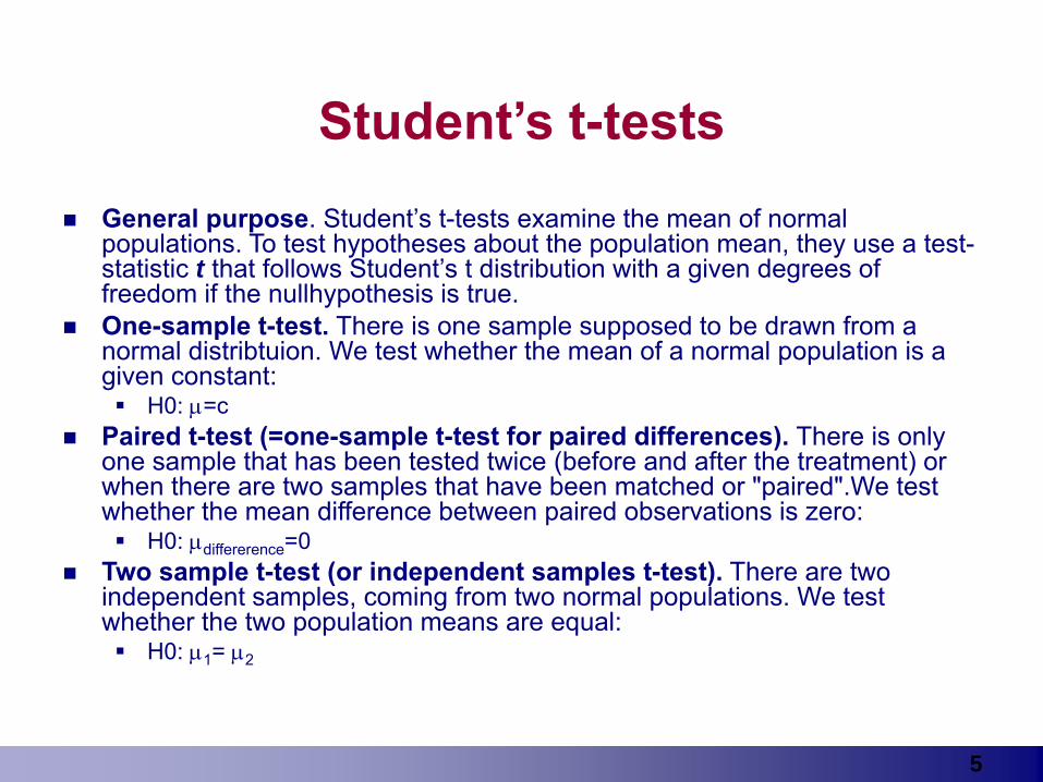
Student’s t-testsGeneral purpose. Student’s t-tests examine the mean of normal populations. To test hypotheses about the population mean, they use a test-statistic t that follows Student’s t distribution with a given degrees of freedom if the nullhypothesis is true.One-sample t-test. There is one sample supposed to be drawn from a normal distribtuion. We test whether the mean of a normal population is a given constant:

H0: μ=cPaired t-test (=one-sample t-test for paired differences). There is only one sample that has been tested twice (before and after the treatment) or when there are two samples that have been matched or "paired".We test whether the mean difference between paired observations is zero:

H0: μdiffererence=0Two sample t-test (or independent samples t-test). There are two independent samples, coming from two normal populations. We test whether the two population means are equal:

H0: μ1= μ2

6

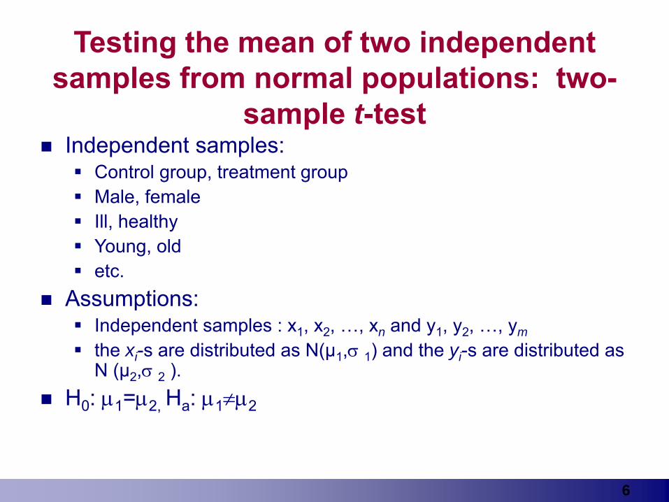
Testing the mean of two independent samples from normal populations: two-

sample t-test Independent samples:

Control group, treatment groupMale, femaleIll, healthyYoung, oldetc.

Assumptions:Independent samples : x1, x2, …, xn and y1, y2, …, ymthe xi-s are distributed as N(µ1,σ 1) and the yi-s are distributed as N (µ2,σ 2 ).

H0: μ1=μ2, Ha: μ1≠μ2

7

Decision rules

Confidence intervals: there are confidence intervals for the difference (we do not study)Critical pointsP-values

If p<0.05, we say that the result is statistically significant at 5% level: i.e. the effect would occur by chance less than 5% of the time

8

Evaluation of two sample t-test depends on equality of variances

9

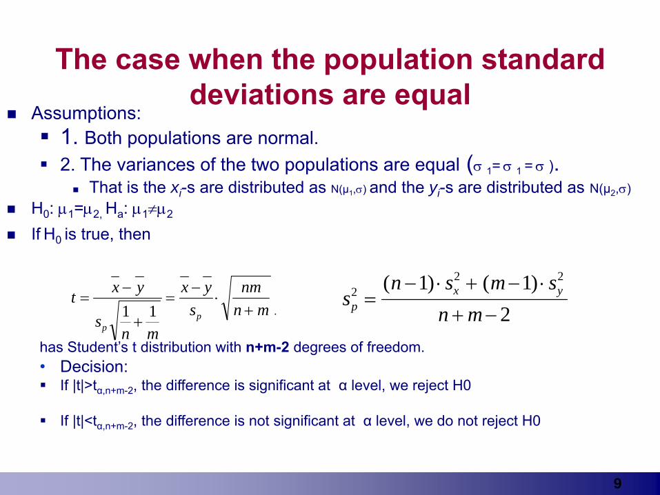
The case when the population standard deviations are equal

Assumptions:1. Both populations are normal.2. The variances of the two populations are equal (σ 1= σ 1 = σ ).

That is the xi-s are distributed as N(µ1,σ) and the yi-s are distributed as N(µ2,σ) H0: μ1=μ2, Ha: μ1≠μ2

If H0 is true, then

has Student’s t distribution with n+m-2 degrees of freedom. • Decision:

If |t|>tα,n+m-2, the difference is significant at α level, we reject H0

If |t|<tα,n+m-2, the difference is not significant at α level, we do not reject H0

t x y

sn m

x ys

nmn m

pp

=−

+=

−⋅

+1 1 .s

n s m sn mp

x y22 21 1

2=

− ⋅ + − ⋅

+ −

( ) ( )

10

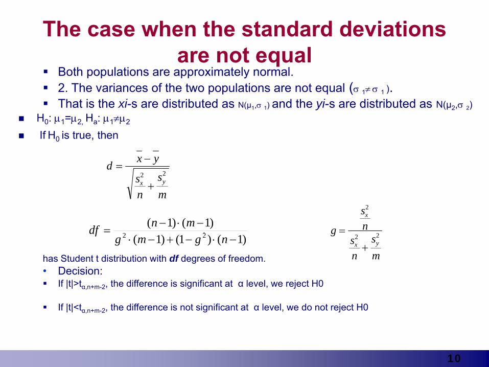
The case when the standard deviations are not equal

Both populations are approximately normal.2. The variances of the two populations are not equal (σ 1≠ σ 1 ). That is the xi-s are distributed as N(µ1,σ 1) and the yi-s are distributed as N(µ2,σ 2)

H0: μ1=μ2, Ha: μ1≠μ2

If H0 is true, then

has Student t distribution with df degrees of freedom. • Decision:

If |t|>tα,n+m-2, the difference is significant at α level, we reject H0

If |t|<tα,n+m-2, the difference is not significant at α level, we do not reject H0

d x y

sn

sm

x y

=−

+2 2

)1()1()1()1()1(

22 −⋅−+−⋅−⋅−

=ngmg

mndf g

sn

sn

sm

x

x y

=+

2

2 2.

11

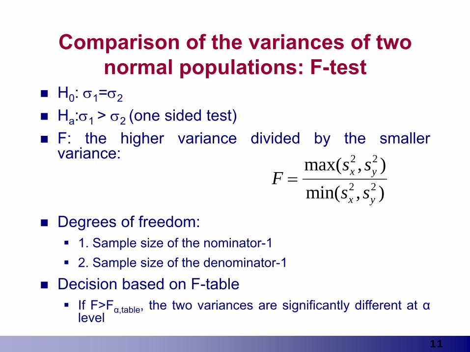
Comparison of the variances of two normal populations: F-test

H0: σ1=σ2

Ha:σ1 > σ2 (one sided test)F: the higher variance divided by the smallervariance:

Degrees of freedom:1. Sample size of the nominator-12. Sample size of the denominator-1

Decision based on F-tableIf F>Fα,table, the two variances are significantly different at αlevel

Fs ss s

x y

x y

=max( , )min( , )

2 2

2 2

12

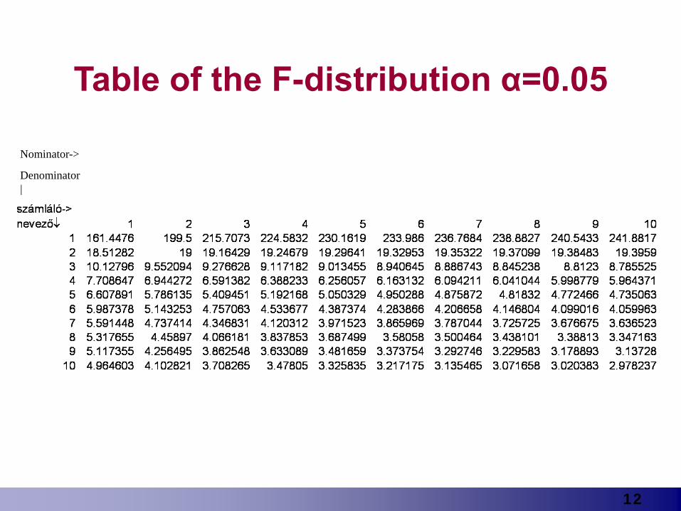
Table of the F-distribution α=0.05

Nominator->

Denominator|

13

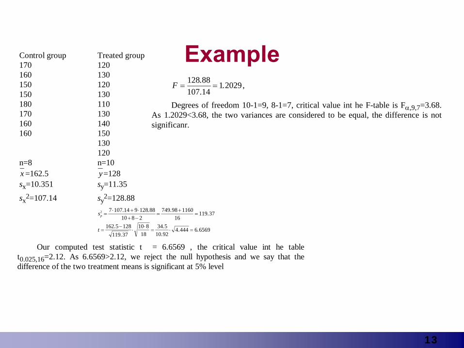
ExampleControl group Treated group 170 120 160 130 150 120 150 130 180 110 170 130 160 140 160 150 130 120 n=8 n=10 x =162.5 y=128 sx=10.351 sy=11.35

sx2=107.14 sy2=128.88

s

t

p2 7 107 14 9 128 88

10 8 2749 98 1160

16119 37

162 5 128119 37

10 818

34 510 92

4 444 6 6569

=⋅ + ⋅

+ −=

+=

=−

⋅⋅

= ⋅ =

. . . .

..

..

. .

Our computed test statistic t = 6.6569 , the critical value int he table t0.025,16=2.12. As 6.6569>2.12, we reject the null hypothesis and we say that the difference of the two treatment means is significant at 5% level

F = =128 88107 14

1 2029..

. ,

Degrees of freedom 10-1=9, 8-1=7, critical value int he F-table is Fα,9,7=3.68. As 1.2029<3.68, the two variances are considered to be equal, the difference is not significanr.

14

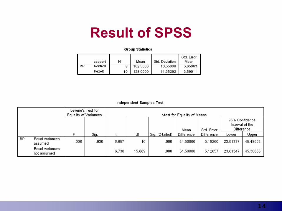
Result of SPSS

15

Two sample t-test, example 2.

A study was conducted to determine weight loss, body composition, etc. in obese women before and after 12 weeks in two groups:Group I. treatment with a very-low-calorie diet . Group II. no diet Volunteers were randomly assigned to one of these groups.We wish to know if these data provide sufficient evidence to allow us to conclude that the treatment is effective in causing weight reduction in obese women compared to no treatment.

16

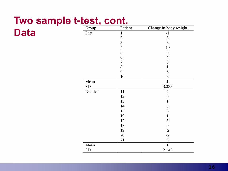
Two sample t-test, cont. Data Group Patient Change in body weight

Diet 1 -1 2 5 3 3 4 10 5 6 6 4 7 0 8 1 9 6 10 6 Mean 4. SD 3.333 No diet 11 2 12 0 13 1 14 0 15 3 16 1 17 5 18 0 19 -2 20 -2 21 3 Mean 1 SD 2.145

17

Two sample t-test, example, cont.

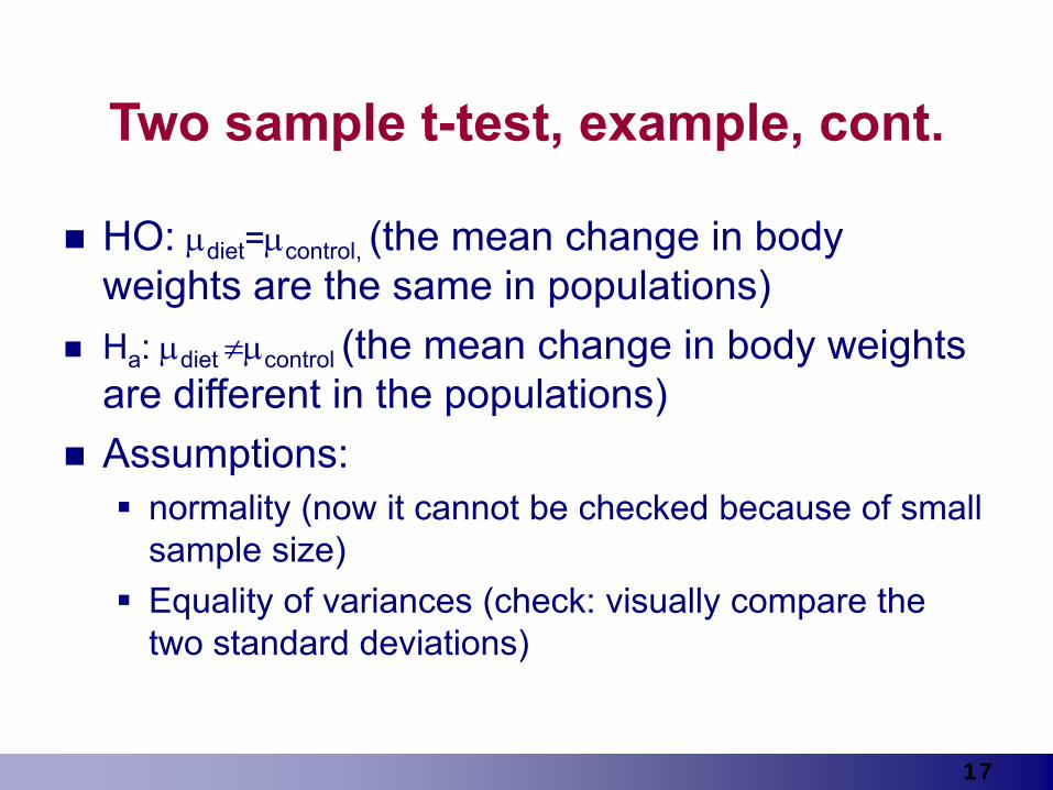
HO: μdiet=μcontrol, (the mean change in body weights are the same in populations) Ha: μdiet ≠μcontrol (the mean change in body weights are different in the populations) Assumptions:

normality (now it cannot be checked because of small sample size)Equality of variances (check: visually compare the two standard deviations)

18

Two sample t-test, example, cont.

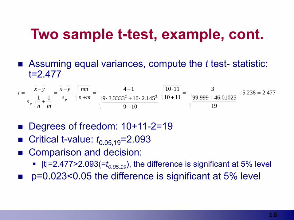
Assuming equal variances, compute the t test- statistic: t=2.477

Degrees of freedom: 10+11-2=19Critical t-value: t0.05,19=2.093 Comparison and decision:

|t|=2.477>2.093(=t0.05,19), the difference is significant at 5% level p=0.023<0.05 the difference is significant at 5% level

477.2238.5

1901025.64999.99

311101110

109145.2103333.39

1411 22

=+

=+⋅

+⋅+⋅

−=

+⋅

−=

+

−=

mnnm

syx

mns

yxtp

p

19

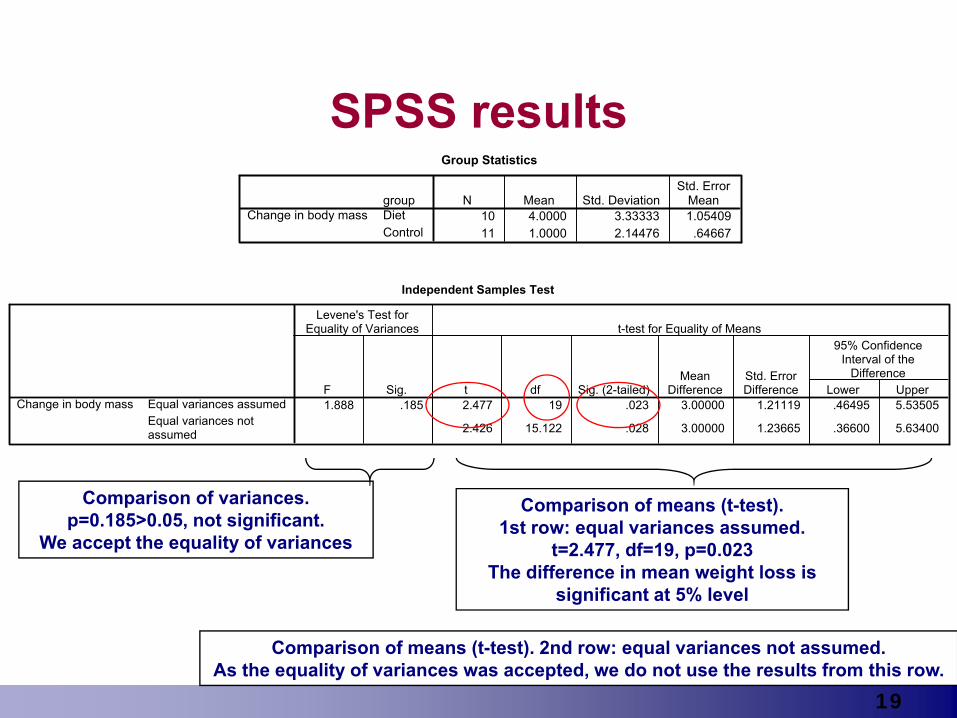
SPSS resultsGroup Statistics

10 4.0000 3.33333 1.0540911 1.0000 2.14476 .64667

groupDietControl

Change in body massN Mean Std. Deviation

Std. ErrorMean

Independent Samples Test

1.888 .185 2.477 19 .023 3.00000 1.21119 .46495 5.53505

2.426 15.122 .028 3.00000 1.23665 .36600 5.63400

Equal variances assumedEqual variances notassumed

Change in body massF Sig.

Levene's Test forEquality of Variances

t df Sig. (2-tailed)Mean

DifferenceStd. ErrorDifference Lower Upper

95% ConfidenceInterval of the

Difference

t-test for Equality of Means

Comparison of variances.p=0.185>0.05, not significant.

We accept the equality of variances

Comparison of means (t-test).1st row: equal variances assumed.

t=2.477, df=19, p=0.023The difference in mean weight loss is

significant at 5% level

Comparison of means (t-test). 2nd row: equal variances not assumed. As the equality of variances was accepted, we do not use the results from this row.

20

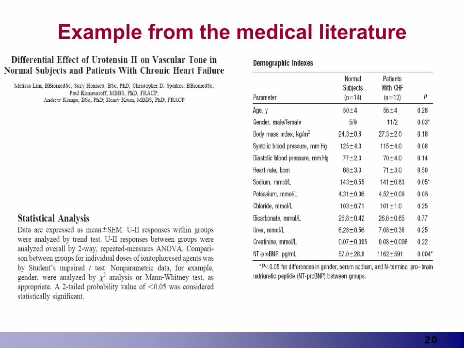
Example from the medical literature

21

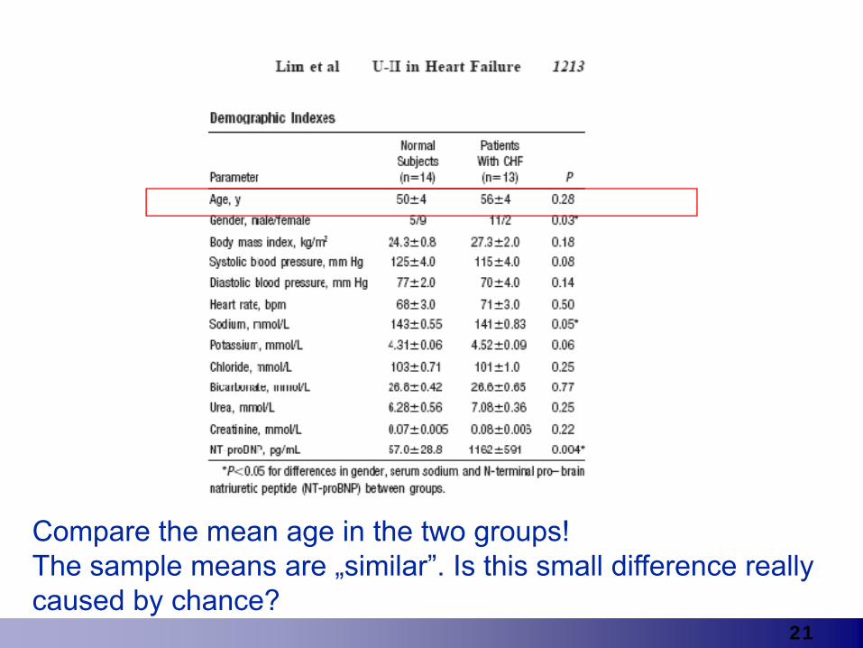
Compare the mean age in the two groups! The sample means are „similar”. Is this small difference really caused by chance?

22

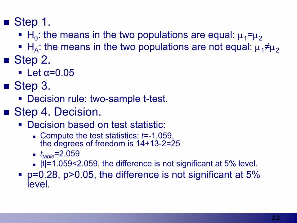
Step 1.H0: the means in the two populations are equal: μ1=μ2HA: the means in the two populations are not equal: μ1≠μ2

Step 2. Let α=0.05

Step 3. Decision rule: two-sample t-test.

Step 4. Decision.Decision based on test statistic:

Compute the test statistics: t=-1.059, the degrees of freedom is 14+13-2=25 ttable=2.059|t|=1.059<2.059, the difference is not significant at 5% level.

p=0.28, p>0.05, the difference is not significant at 5% level.

23

How to get the p-value?

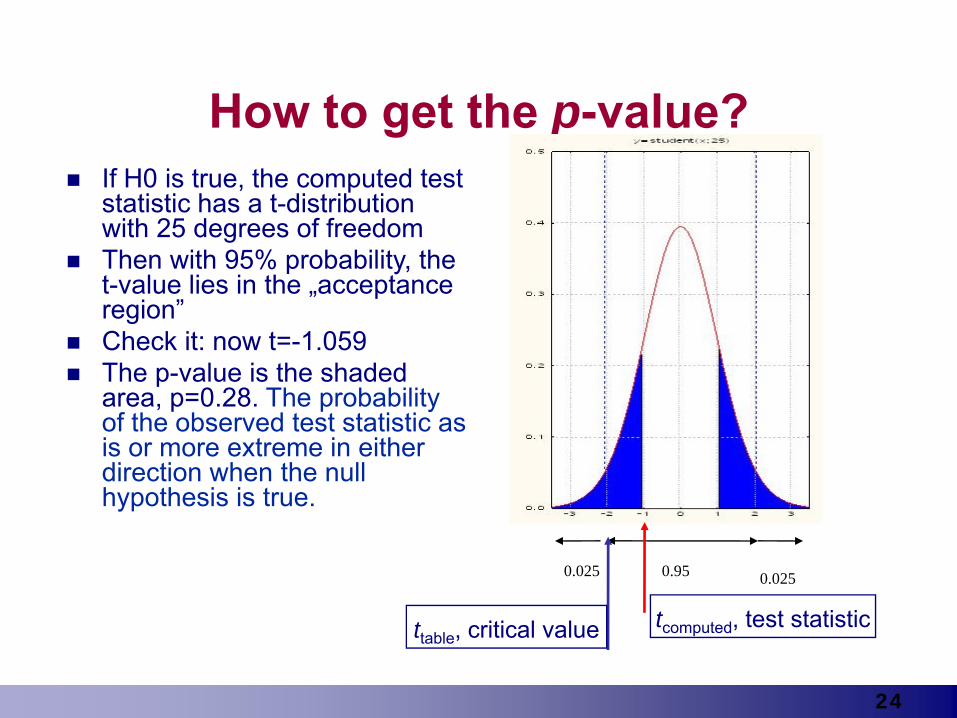
If H0 is true, the computed test statistic has a t-distribution with 25 degrees of freedom.Then with 95% probability, the t-value lies in the „acceptance region”Check it: now t=-1.059

0.025 0.0250.95

ttable, critical value

24

How to get the p-value?If H0 is true, the computed test statistic has a t-distribution with 25 degrees of freedomThen with 95% probability, the t-value lies in the „acceptance region”Check it: now t=-1.059The p-value is the shaded area, p=0.28. The probability of the observed test statistic as is or more extreme in either direction when the null hypothesis is true.

0.025 0.0250.95

ttable, critical value tcomputed, test statistic

25

How to get the t-value using statistical software – given sample size, sample

mean and sample SD?

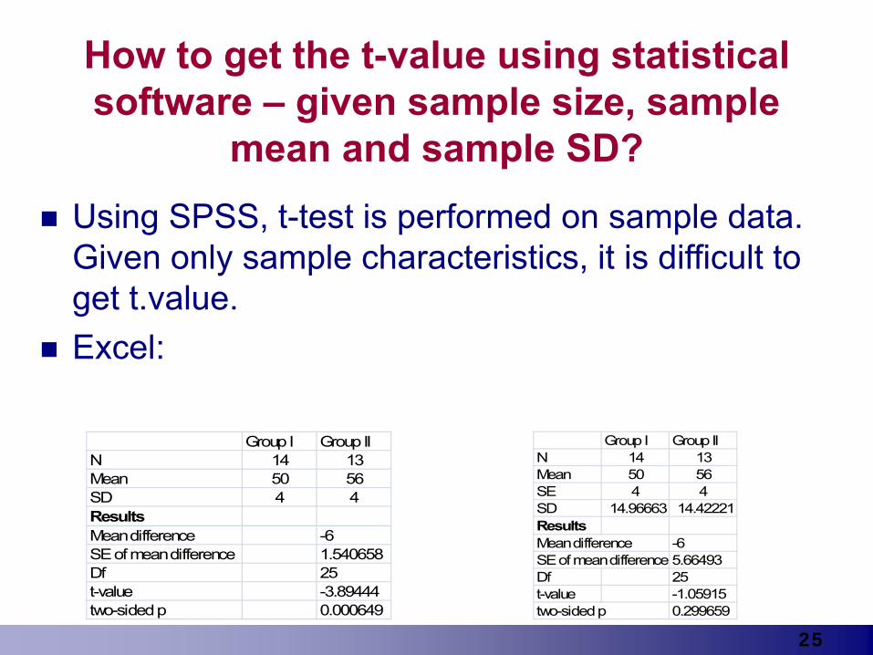
Group I Group IIN 14 13Mean 50 56SD 4 4ResultsMean difference -6SE of mean difference 1.540658Df 25t-value -3.89444two-sided p 0.000649

Group I Group IIN 14 13Mean 50 56SE 4 4SD 14.96663 14.42221ResultsMean difference -6SE of mean difference 5.66493Df 25t-value -1.05915two-sided p 0.299659

Using SPSS, t-test is performed on sample data. Given only sample characteristics, it is difficult to get t.value.Excel:

26

Answer to the motivated example (mean age of boys and girls)

Group Statistics

84 21.18 3.025 .33053 20.38 3.108 .427

SexMaleFemale

Age in yearsN Mean Std. Deviation

Std. ErrorMean

Independent Samples Test

.109 .741 1.505 135 .135 .807 .536 -.253 1.868

1.496 108.444 .138 .807 .540 -.262 1.877

Equal variances assumedEqual variances notassumed

Age in yearsF Sig.

Levene's Test forEquality of Variances

t df Sig. (2-tailed)Mean

DifferenceStd. ErrorDifference Lower Upper

95% ConfidenceInterval of the

Difference

t-test for Equality of Means

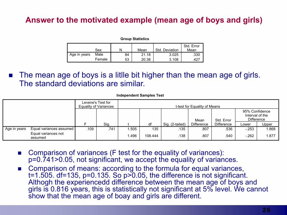
Comparison of variances (F test for the equality of variances): p=0.741>0.05, not significant, we accept the equality of variances.Comparison of means: according to the formula for equal variances, t=1.505. df=135, p=0.135. So p>0.05, the difference is not significant. Althogh the experiencedd difference between the mean age of boys and girls is 0.816 years, this is statistically not significant at 5% level. We cannot show that the mean age of boay and girls are different.

The mean age of boys is a litlle bit higher than the mean age of girls. The standard deviations are similar.

27

Other aspects of statistical tests

28

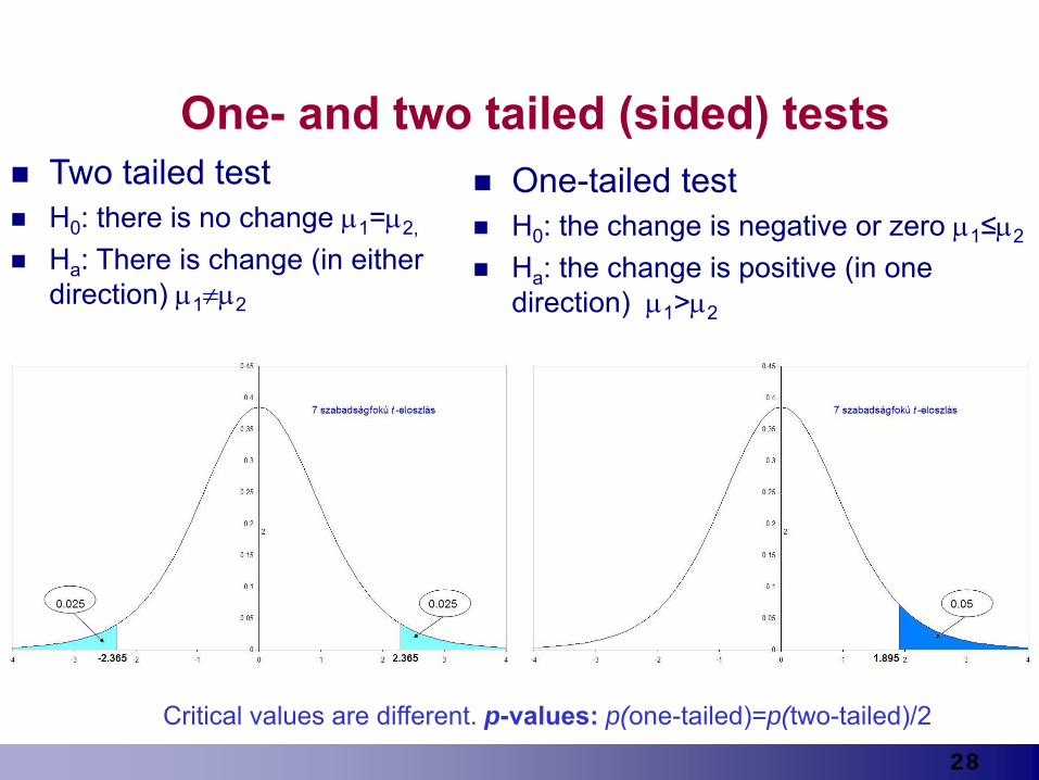
One- and two tailed (sided) testsTwo tailed testH0: there is no change μ1=μ2,

Ha: There is change (in either direction) μ1≠μ2

One-tailed testH0: the change is negative or zero μ1≤μ2

Ha: the change is positive (in one direction) μ1>μ2

Critical values are different. p-values: p(one-tailed)=p(two-tailed)/2

29

SignificanceSignificant difference – if we claim that there is a difference (effect), the probability of mistake is small (maximum α- Type I error ).Not significant difference – we say that there is not enough information to show difference. Perhaps

there is no difference There is a difference but the sample size is smallThe dispersion is bigThe method was wrong

Even is case of a statistically significant difference one has to think about its biological meaning

30

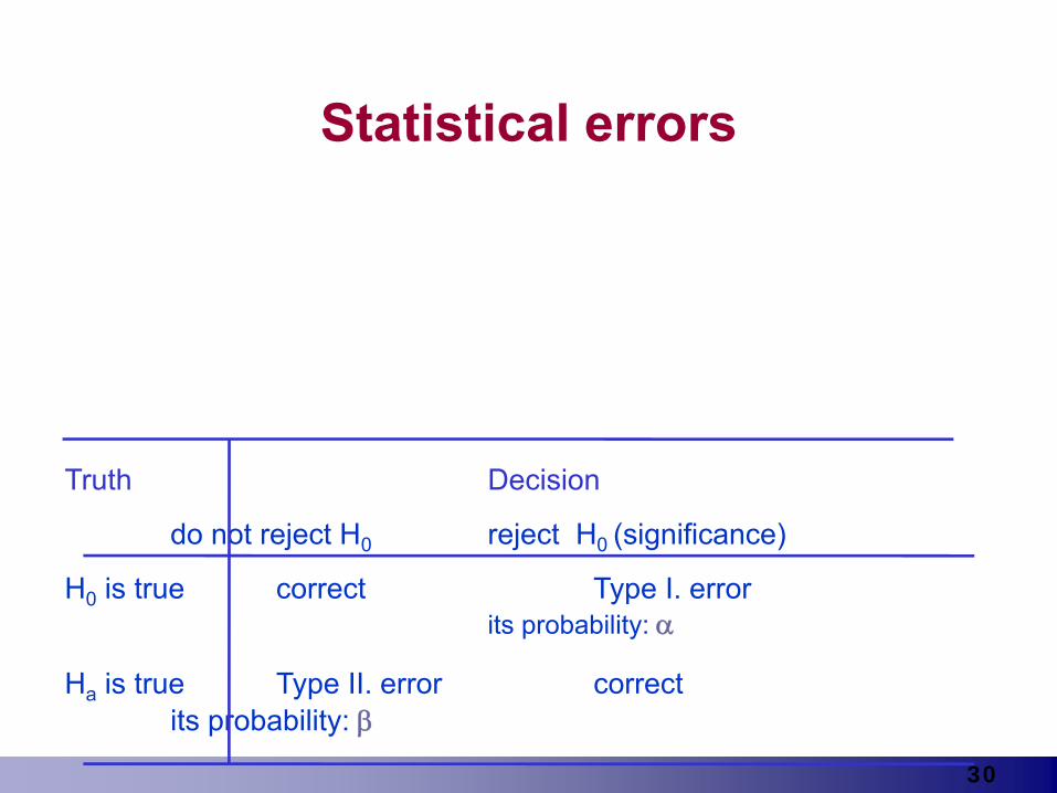
Statistical errors

Truth Decision

do not reject H0 reject H0 (significance)

H0 is true correct Type I. errorits probability: α

Ha is true Type II. error correctits probability: β

31

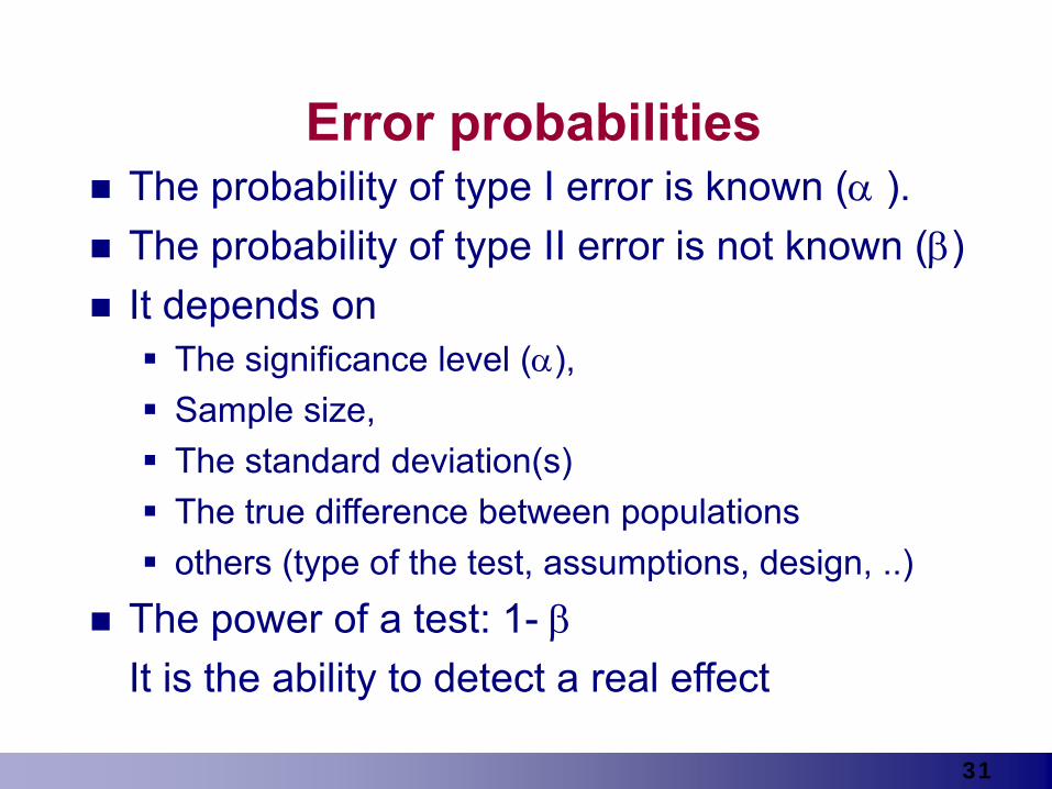
Error probabilitiesThe probability of type I error is known (α ).The probability of type II error is not known (β) It depends on

The significance level (α), Sample size, The standard deviation(s) The true difference between populationsothers (type of the test, assumptions, design, ..)

The power of a test: 1- βIt is the ability to detect a real effect

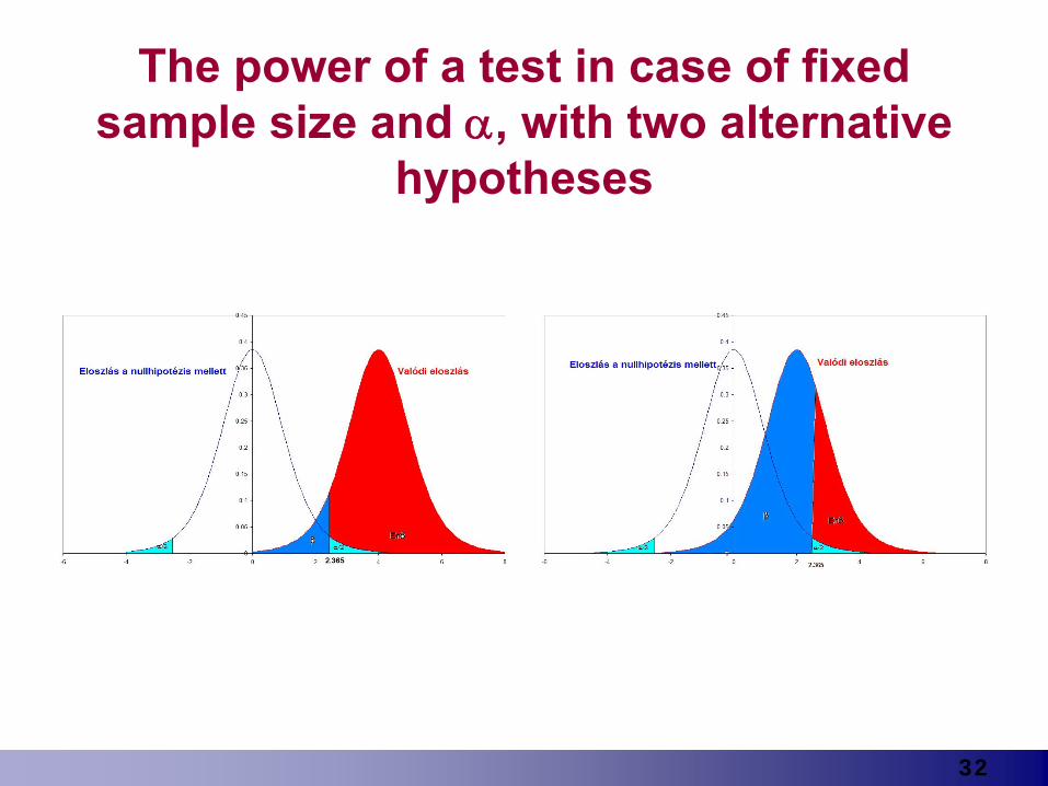
32

The power of a test in case of fixed sample size and α, with two alternative

hypotheses

33

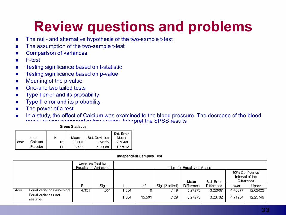
Review questions and problemsThe null- and alternative hypothesis of the two-sample t-testThe assumption of the two-sample t-testComparison of variancesF-testTesting significance based on t-statisticTesting significance based on p-valueMeaning of the p-valueOne-and two tailed testsType I error and its probabilityType II error and its probabilityThe power of a testIn a study, the effect of Calcium was examined to the blood pressure. The decrease of the blood pressure was compared in two groups. Interpret the SPSS results

Group Statistics

10 5.0000 8.74325 2.7648611 -.2727 5.90069 1.77913

treatCalciumPlacebo

decrN Mean Std. Deviation

Std. ErrorMean

Independent Samples Test

4.351 .051 1.634 19 .119 5.27273 3.22667 -1.48077 12.02622

1.604 15.591 .129 5.27273 3.28782 -1.71204 12.25749

Equal variances assumedEqual variances notassumed

decrF Sig.

Levene's Test forEquality of Variances

t df Sig. (2-tailed)Mean

DifferenceStd. ErrorDifference Lower Upper

95% ConfidenceInterval of the

Difference

t-test for Equality of Means