Hypothesis tests. One- and two sample t-tests. fileTwo sample t-test (or independent samples t-test). There are two independent samples, coming from two normal populations. We test

BiostatisticsHypothesis tests.

One- and two sample t-tests.

Krisztina Boda PhD

Department of Medical Physics and

Informatics, University of Szeged

Krisztina Boda 2

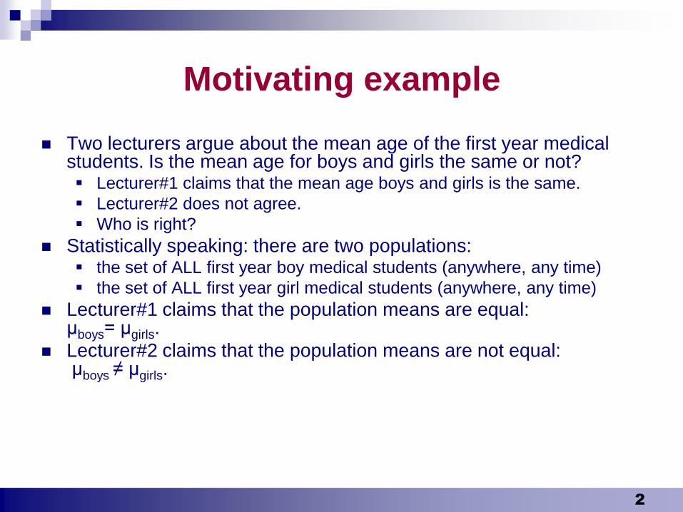
Motivating example

Two lecturers argue about the mean age of the first year medical students. Is the mean age for boys and girls the same or not? Lecturer#1 claims that the mean age boys and girls is the same.

Lecturer#2 does not agree.

Who is right?

Statistically speaking: there are two populations: the set of ALL first year boy medical students (anywhere, any time)

the set of ALL first year girl medical students (anywhere, any time)

Lecturer#1 claims that the population means are equal: μboys= μgirls.

Lecturer#2 claims that the population means are not equal:μboys ≠ μgirls.

Krisztina Boda 3

Independent samples

compare males and females

compare two populations receiving

different treatments

compare healthy and ill patients

compare young and old patients

……

Krisztina Boda 4

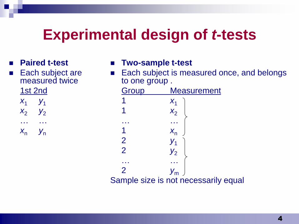
Experimental design of t-tests

Paired t-test

Each subject are measured twice

1st 2nd

x1 y1

x2 y2

… …

xn yn

Two-sample t-test

Each subject is measured once, and belongs to one group .

Group Measurement

1 x1

1 x2

… …

1 xn

2 y1

2 y2

… …

2 ym

Sample size is not necessarily equal

Krisztina Boda 5

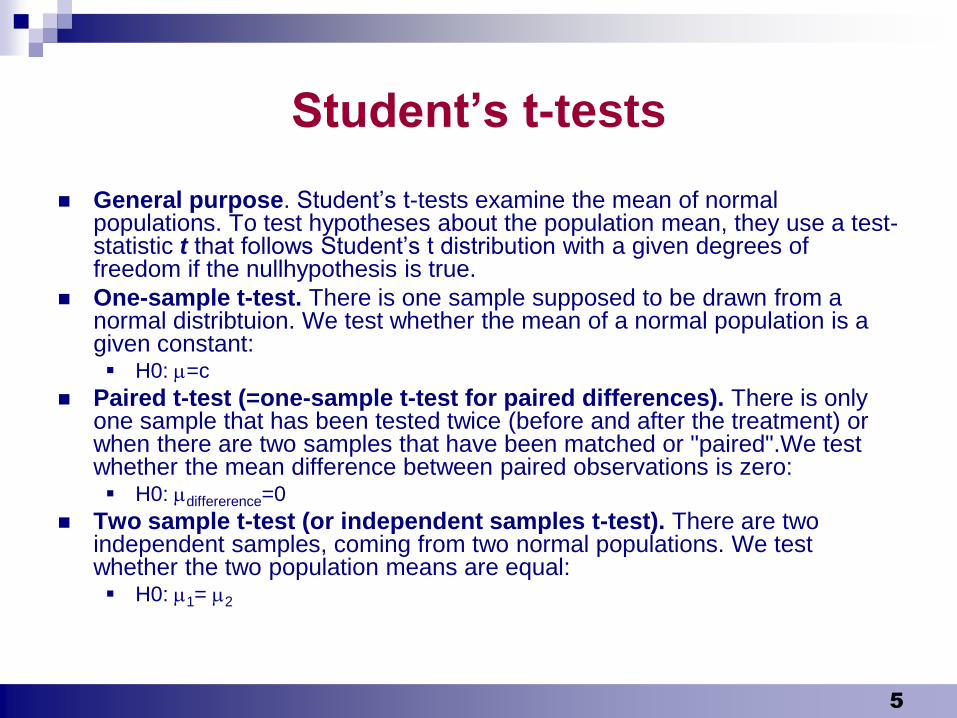
Student’s t-tests

General purpose. Student’s t-tests examine the mean of normal populations. To test hypotheses about the population mean, they use a test-statistic t that follows Student’s t distribution with a given degrees of freedom if the nullhypothesis is true.

One-sample t-test. There is one sample supposed to be drawn from a normal distribtuion. We test whether the mean of a normal population is a given constant: H0: =c

Paired t-test (=one-sample t-test for paired differences). There is only one sample that has been tested twice (before and after the treatment) or when there are two samples that have been matched or "paired".We test whether the mean difference between paired observations is zero: H0: differerence=0

Two sample t-test (or independent samples t-test). There are two independent samples, coming from two normal populations. We test whether the two population means are equal: H0: 1= 2

Krisztina Boda 6

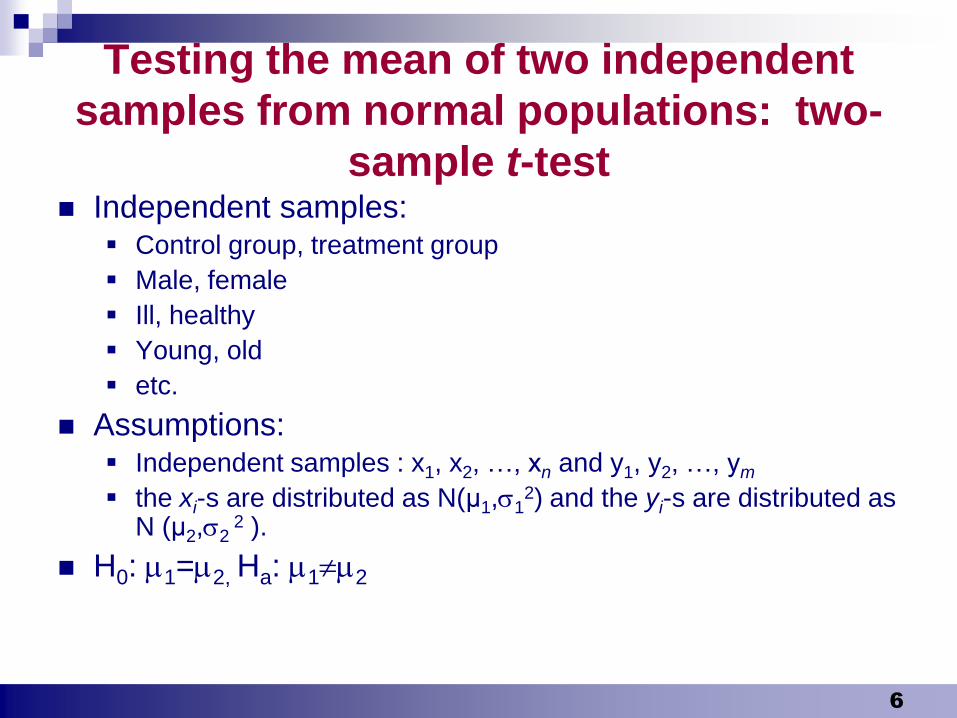
Testing the mean of two independent

samples from normal populations: two-

sample t-test Independent samples:

Control group, treatment group

Male, female

Ill, healthy

Young, old

etc.

Assumptions: Independent samples : x1, x2, …, xn and y1, y2, …, ym

the xi-s are distributed as N(µ1,12) and the yi-s are distributed as

N (µ2,22 ).

H0: 1=2, Ha: 12

Krisztina Boda 7

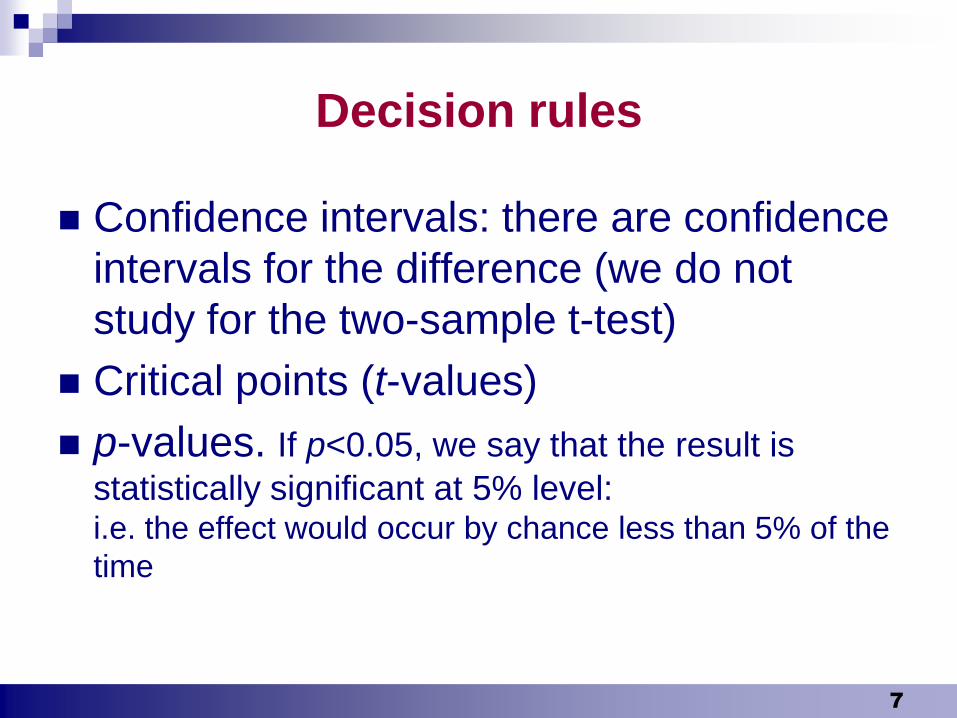
Decision rules

Confidence intervals: there are confidence

intervals for the difference (we do not

study for the two-sample t-test)

Critical points (t-values)

p-values. If p<0.05, we say that the result is

statistically significant at 5% level: i.e. the effect would occur by chance less than 5% of the

time

Krisztina Boda 8

Evaluation of two sample t-test depends on

equality of variances;

To compare the means, there are two different

formulas with different degrees of freedom

depending on equality of variances

Krisztina Boda 9

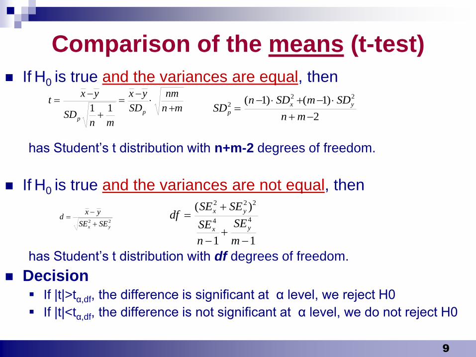
Comparison of the means (t-test)

If H0 is true and the variances are equal, then

has Student’s t distribution with n+m-2 degrees of freedom.

If H0 is true and the variances are not equal, then

has Student’s t distribution with df degrees of freedom.

Decision If |t|>tα,df, the difference is significant at α level, we reject H0

If |t|<tα,df, the difference is not significant at α level, we do not reject H0

mn

nm

SD

yx

mnSD

yxt

pp

11

.

2

)1()1( 22

2

mn

SDmSDnSD

yx

p

22

yx SESE

yxd

11

)(44

222

m

SE

n

SE

SESEdf

yx

yx

Krisztina Boda

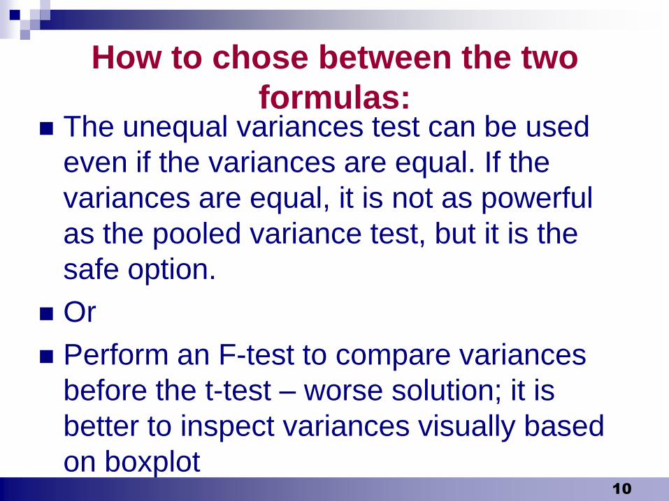
How to chose between the two

formulas: The unequal variances test can be used

even if the variances are equal. If the

variances are equal, it is not as powerful

as the pooled variance test, but it is the

safe option.

Or

Perform an F-test to compare variances

before the t-test – worse solution; it is

better to inspect variances visually based

on boxplot10

Krisztina Boda 11

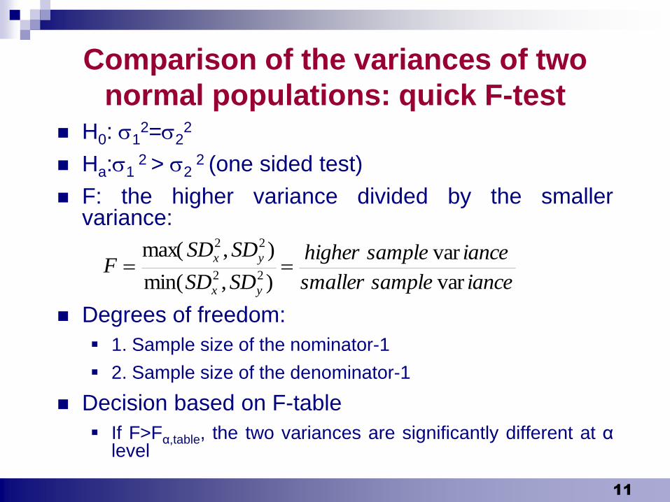
Comparison of the variances of two

normal populations: quick F-test H0: 1

2=22

Ha:12 > 2

2 (one sided test)

F: the higher variance divided by the smallervariance:

Degrees of freedom:

1. Sample size of the nominator-1

2. Sample size of the denominator-1

Decision based on F-table

If F>Fα,table, the two variances are significantly different at αlevel

iancesamplesmaller

iancesamplehigher

SDSD

SDSDF

yx

yx

var

var

),min(

),max(22

22

Krisztina Boda 12

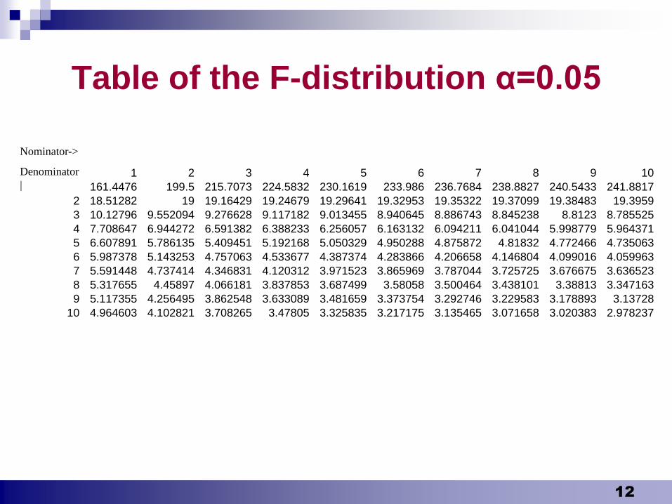
Table of the F-distribution α=0.05

számláló->

nevező 1 2 3 4 5 6 7 8 9 10

1 161.4476 199.5 215.7073 224.5832 230.1619 233.986 236.7684 238.8827 240.5433 241.8817

2 18.51282 19 19.16429 19.24679 19.29641 19.32953 19.35322 19.37099 19.38483 19.3959

3 10.12796 9.552094 9.276628 9.117182 9.013455 8.940645 8.886743 8.845238 8.8123 8.785525

4 7.708647 6.944272 6.591382 6.388233 6.256057 6.163132 6.094211 6.041044 5.998779 5.964371

5 6.607891 5.786135 5.409451 5.192168 5.050329 4.950288 4.875872 4.81832 4.772466 4.735063

6 5.987378 5.143253 4.757063 4.533677 4.387374 4.283866 4.206658 4.146804 4.099016 4.059963

7 5.591448 4.737414 4.346831 4.120312 3.971523 3.865969 3.787044 3.725725 3.676675 3.636523

8 5.317655 4.45897 4.066181 3.837853 3.687499 3.58058 3.500464 3.438101 3.38813 3.347163

9 5.117355 4.256495 3.862548 3.633089 3.481659 3.373754 3.292746 3.229583 3.178893 3.13728

10 4.964603 4.102821 3.708265 3.47805 3.325835 3.217175 3.135465 3.071658 3.020383 2.978237

Nominator->

Denominator

|

Krisztina Boda 13

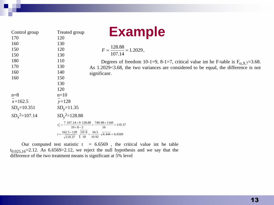
ExampleControl group Treated group

170 120

160 130

150 120

150 130

180 110

170 130

160 140

160 150

130

120

n=8 n=10

x=162.5 y=128

SDx=10.351 SDy=11.35

SDx2=107.14 SDy

2=128.88

s

t

p

2 7 107 14 9 128 88

10 8 2

749 98 1160

16119 37

162 5 128

119 37

10 8

18

34 5

10 924 444 6 6569

. . ..

.

.

.

.. .

Our computed test statistic t = 6.6569 , the critical value int he table

t0.025,16=2.12. As 6.6569>2.12, we reject the null hypothesis and we say that the

difference of the two treatment means is significant at 5% level

F 128 88

107 141 2029

.

.. ,

Degrees of freedom 10-1=9, 8-1=7, critical value int he F-table is F,9,7=3.68.

As 1.2029<3.68, the two variances are considered to be equal, the difference is not

significanr.

Krisztina Boda 14

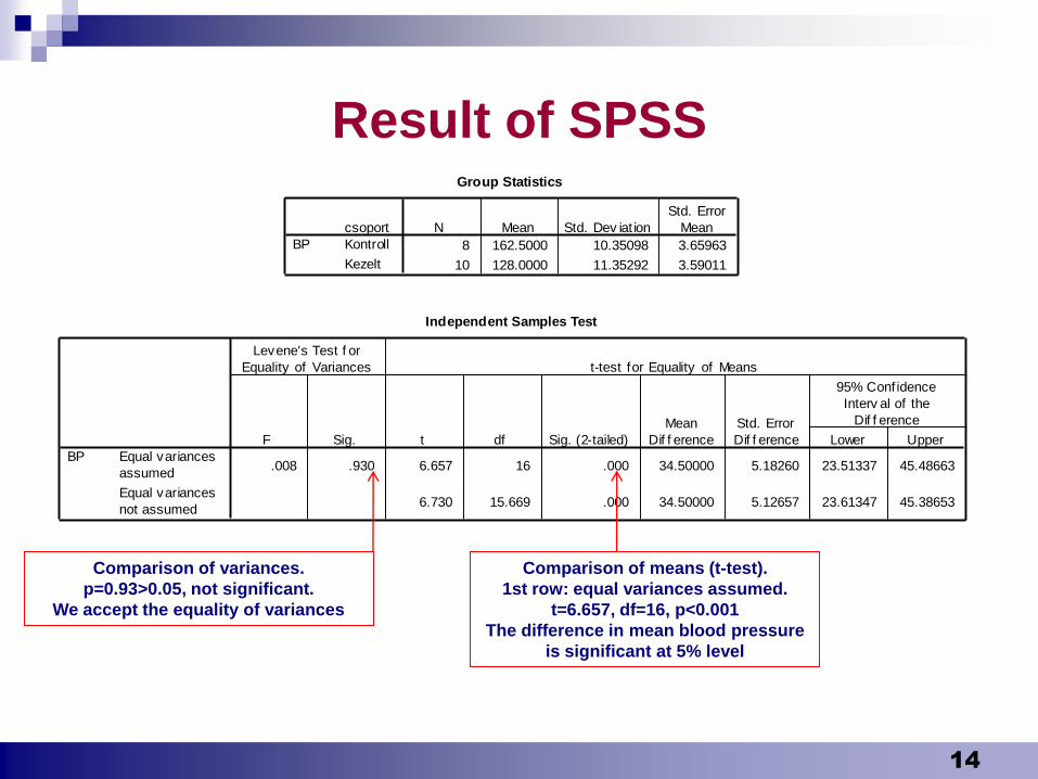
Result of SPSSGroup Statistics

8 162.5000 10.35098 3.65963

10 128.0000 11.35292 3.59011

csoport

Kontroll

Kezelt

BP

N Mean Std. Dev iat ion

Std. Error

Mean

Independent Samples Test

.008 .930 6.657 16 .000 34.50000 5.18260 23.51337 45.48663

6.730 15.669 .000 34.50000 5.12657 23.61347 45.38653

Equal variances

assumed

Equal variances

not assumed

BP

F Sig.

Levene's Test f or

Equality of Variances

t df Sig. (2-tailed)

Mean

Dif f erence

Std. Error

Dif f erence Lower Upper

95% Conf idence

Interv al of the

Dif f erence

t-test for Equality of Means

Comparison of variances.

p=0.93>0.05, not significant.

We accept the equality of variances

Comparison of means (t-test).

1st row: equal variances assumed.

t=6.657, df=16, p<0.001

The difference in mean blood pressure

is significant at 5% level

Krisztina Boda 15

Two sample t-test, example 2.

A study was conducted to determine weight loss, body composition, etc. in obese women before and after 12 weeks in two groups:

Group I. treatment with a very-low-calorie diet .

Group II. no diet

Volunteers were randomly assigned to one of these groups.

We wish to know if these data provide sufficient evidence to allow us to conclude that the treatment is effective in causing weight reduction in obese women compared to no treatment.

Krisztina Boda 16

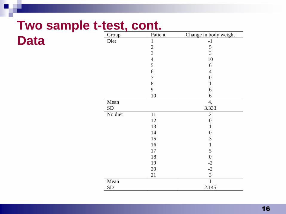
Two sample t-test, cont.

DataGroup Patient Change in body weight

Diet 1 -1

2 5

3 3

4 10

5 6

6 4

7 0

8 1

9 6

10 6

Mean 4.

SD 3.333

No diet 11 2

12 0

13 1

14 0

15 3

16 1

17 5

18 0

19 -2

20 -2

21 3

Mean 1

SD 2.145

Krisztina Boda 17

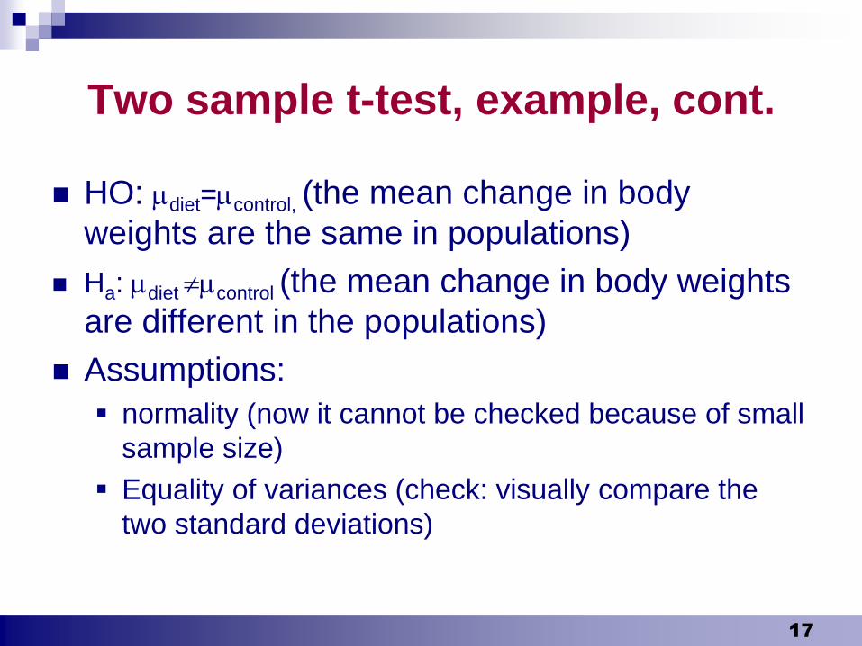
Two sample t-test, example, cont.

HO: diet=control, (the mean change in body

weights are the same in populations)

Ha: diet control (the mean change in body weights

are different in the populations)

Assumptions:

normality (now it cannot be checked because of small

sample size)

Equality of variances (check: visually compare the

two standard deviations)

Krisztina Boda 18

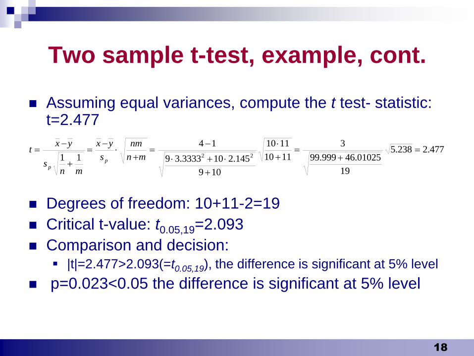
Two sample t-test, example, cont.

Assuming equal variances, compute the t test- statistic: t=2.477

Degrees of freedom: 10+11-2=19

Critical t-value: t0.05,19=2.093

Comparison and decision: |t|=2.477>2.093(=t0.05,19), the difference is significant at 5% level

p=0.023<0.05 the difference is significant at 5% level

477.2238.5

19

01025.64999.99

3

1110

1110

109

145.2103333.39

14

11 22

mn

nm

s

yx

mns

yxt

p

p

Krisztina Boda 19

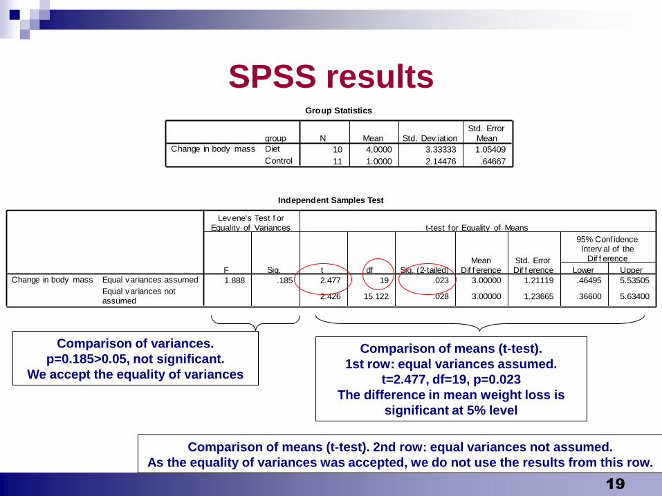
SPSS resultsGroup Statistics

10 4.0000 3.33333 1.05409

11 1.0000 2.14476 .64667

group

Diet

Control

Change in body mass

N Mean Std. Dev iat ionStd. Error

Mean


1.888 .185 2.477 19 .023 3.00000 1.21119 .46495 5.53505

2.426 15.122 .028 3.00000 1.23665 .36600 5.63400

Equal variances assumed

Equal variances notassumed

Change in body massF Sig.

Levene's Test f orEquality of Variances

t df Sig. (2-tailed)Mean

Dif f erenceStd. ErrorDif f erence Lower Upper

95% Conf idenceInterv al of the

Dif f erence


Comparison of variances.

p=0.185>0.05, not significant.

We accept the equality of variances

Comparison of means (t-test).

1st row: equal variances assumed.

t=2.477, df=19, p=0.023

The difference in mean weight loss is

significant at 5% level

Comparison of means (t-test). 2nd row: equal variances not assumed.

As the equality of variances was accepted, we do not use the results from this row.

Krisztina Boda 20

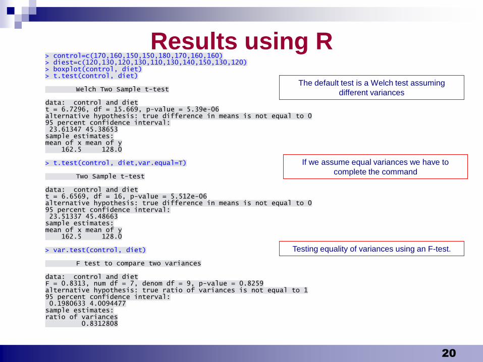
Results using R> control=c(170,160,150,150,180,170,160,160) > diest=c(120,130,120,130,110,130,140,150,130,120) > boxplot(control, diet) > t.test(control, diet) Welch Two Sample t-test data: control and diet t = 6.7296, df = 15.669, p-value = 5.39e-06 alternative hypothesis: true difference in means is not equal to 0 95 percent confidence interval: 23.61347 45.38653 sample estimates: mean of x mean of y 162.5 128.0 > t.test(control, diet,var.equal=T) Two Sample t-test data: control and diet t = 6.6569, df = 16, p-value = 5.512e-06 alternative hypothesis: true difference in means is not equal to 0 95 percent confidence interval: 23.51337 45.48663 sample estimates: mean of x mean of y 162.5 128.0 > var.test(control, diet) F test to compare two variances data: control and diet F = 0.8313, num df = 7, denom df = 9, p-value = 0.8259 alternative hypothesis: true ratio of variances is not equal to 1 95 percent confidence interval: 0.1980633 4.0094477 sample estimates: ratio of variances 0.8312808

The default test is a Welch test assuming

different variances

If we assume equal variances we have to

complete the command

Testing equality of variances using an F-test.

Krisztina Boda 21

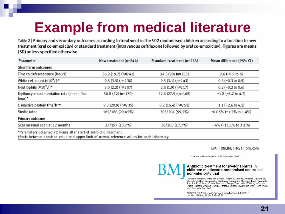
Example from medical literature

Krisztina Boda 22

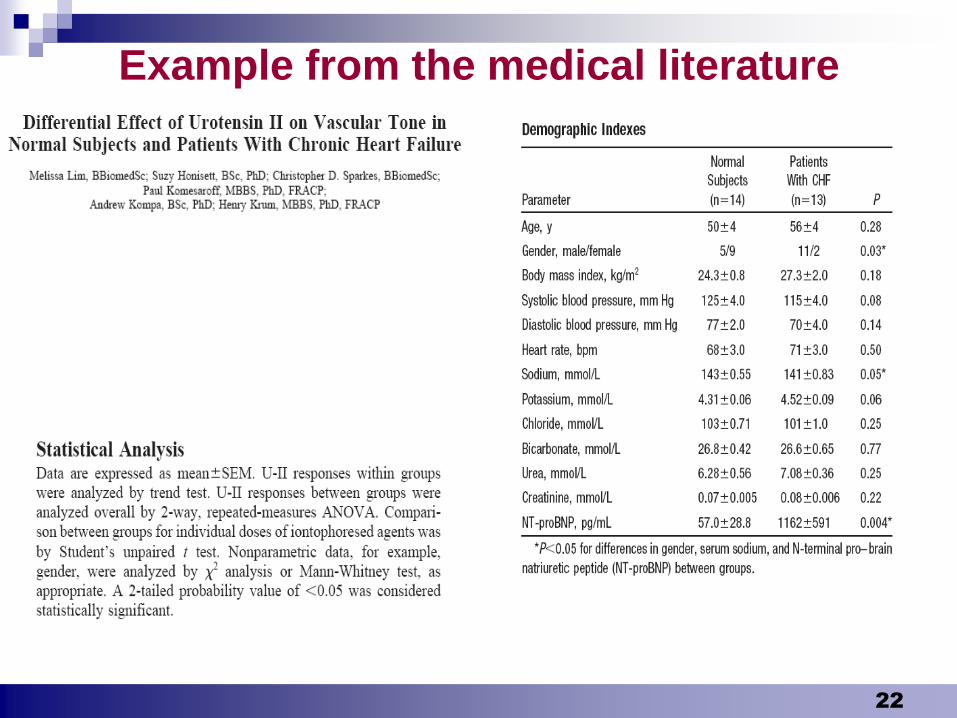
Example from the medical literature

Krisztina Boda 23

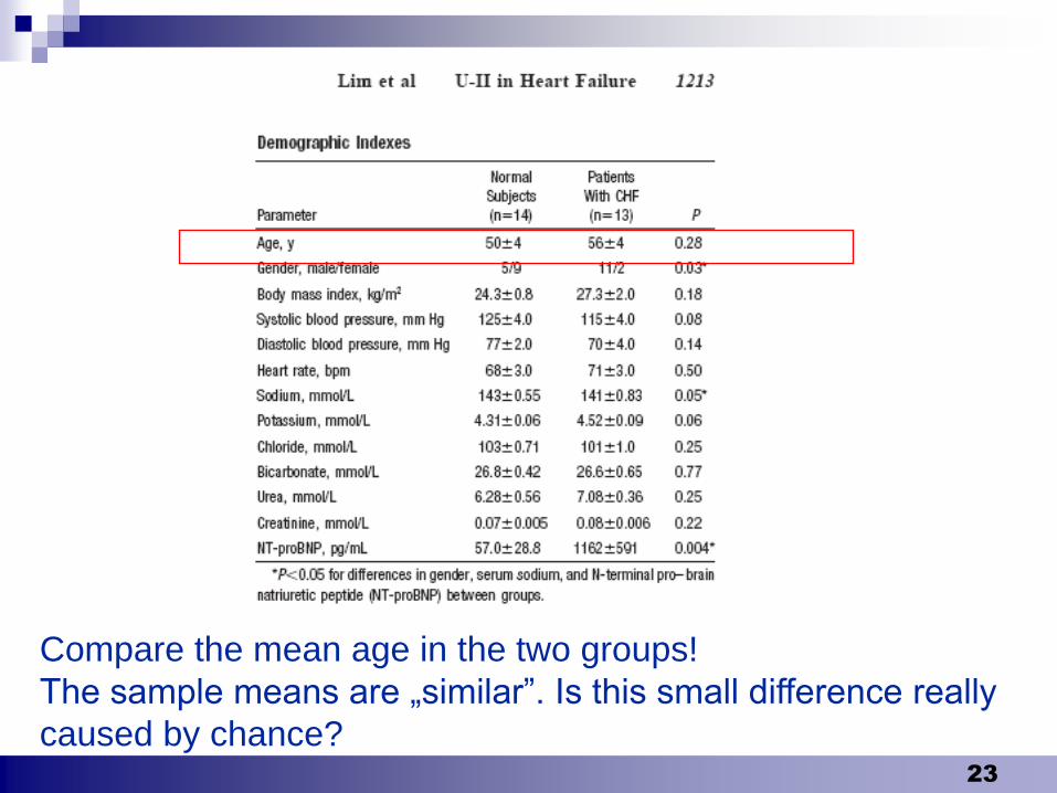
Compare the mean age in the two groups!

The sample means are „similar”. Is this small difference really

caused by chance?

Krisztina Boda 24

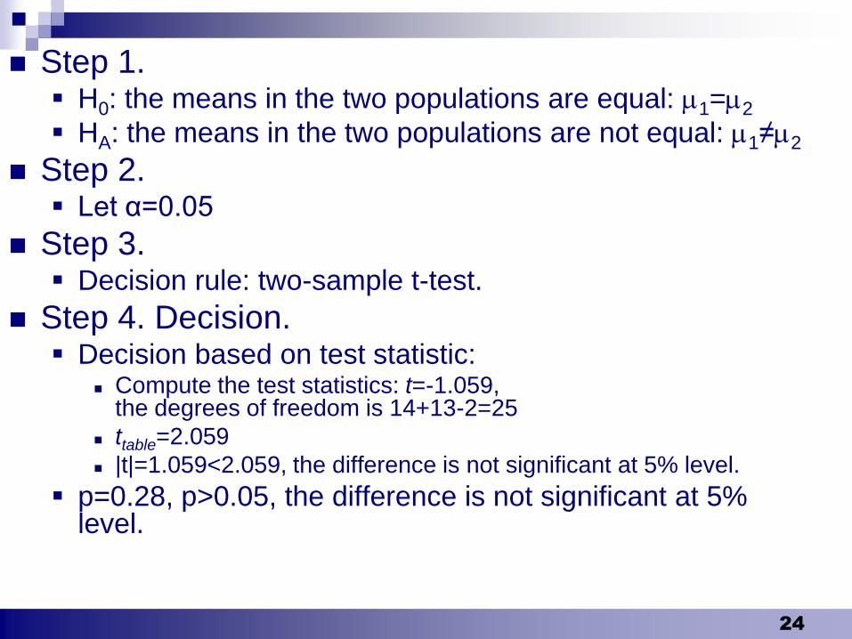
Step 1. H0: the means in the two populations are equal: 1=2

HA: the means in the two populations are not equal: 1≠2

Step 2. Let α=0.05

Step 3. Decision rule: two-sample t-test.

Step 4. Decision. Decision based on test statistic:

Compute the test statistics: t=-1.059, the degrees of freedom is 14+13-2=25

ttable=2.059

|t|=1.059<2.059, the difference is not significant at 5% level.

p=0.28, p>0.05, the difference is not significant at 5% level.

Krisztina Boda 25

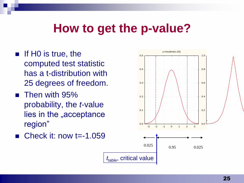
How to get the p-value?

If H0 is true, the

computed test statistic

has a t-distribution with

25 degrees of freedom.

Then with 95%

probability, the t-value

lies in the „acceptance

region”

Check it: now t=-1.0590.025

0.0250.95

y=student(x;25)

-3 -2 -1 0 1 2 3

0.0

0.1

0.2

0.3

0.4

0.5

p=2*(1-istudent(abs(x);25))

-3 -2 -1 0 1 2 3

0.0

0.2

0.4

0.6

0.8

1.0

ttable, critical value

Krisztina Boda 26

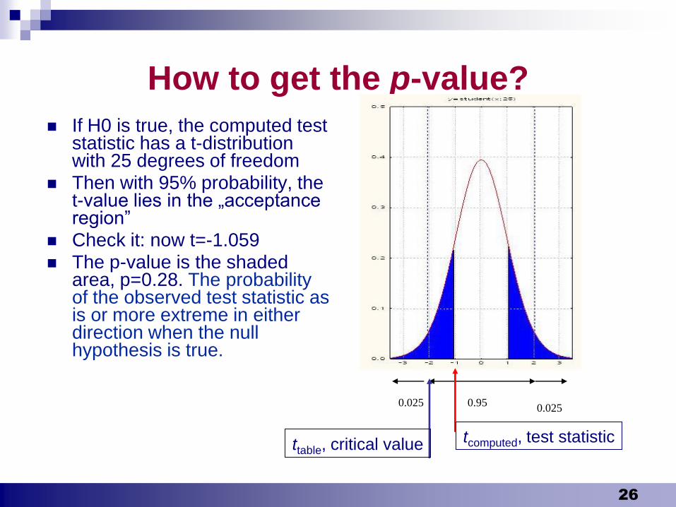
How to get the p-value?

If H0 is true, the computed test statistic has a t-distribution with 25 degrees of freedom

Then with 95% probability, the t-value lies in the „acceptance region”

Check it: now t=-1.059 The p-value is the shaded

area, p=0.28. The probability of the observed test statistic as is or more extreme in either direction when the null hypothesis is true.

0.0250.025

0.95

ttable, critical value tcomputed, test statistic

Krisztina Boda 27

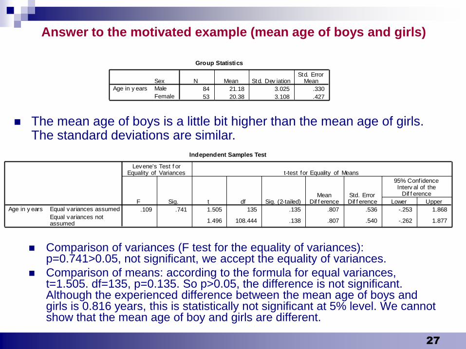
Answer to the motivated example (mean age of boys and girls)

Group Statistics

84 21.18 3.025 .330

53 20.38 3.108 .427

Sex

Male

Female

Age in y ears

N Mean Std. Dev iationStd. Error

Mean


.109 .741 1.505 135 .135 .807 .536 -.253 1.868

1.496 108.444 .138 .807 .540 -.262 1.877



Age in y ears

F Sig.





Dif f erence


Comparison of variances (F test for the equality of variances): p=0.741>0.05, not significant, we accept the equality of variances.

Comparison of means: according to the formula for equal variances, t=1.505. df=135, p=0.135. So p>0.05, the difference is not significant. Although the experienced difference between the mean age of boys and girls is 0.816 years, this is statistically not significant at 5% level. We cannot show that the mean age of boy and girls are different.

The mean age of boys is a little bit higher than the mean age of girls. The standard deviations are similar.

Krisztina Boda 28

Review questions and problems The null- and alternative hypothesis of the two-sample t-test

The assumptions of the two-sample t-test

Comparison of variances

F-test

Testing significance based on t-statistic

Testing significance based on p-value

Meaning of the p-value

One-and two tailed tests

Type I error and its probability

Type II error and its probability

The power of a test

On the physics practicals the body mass was measured. The measurement was repeated three times, the change of the first and second repetitions were compared. The mean differnce was 0.0127 kg, the SE of the mean difference was 0.0354, n=362. The p-value of the test was 0.72. Is there a significant change in mean the body mass at 5% level?

In a study, the effect of Calcium was examined to the blood pressure. The decrease of the blood pressure was compared in two groups. Interpret the SPSS results

Group Statistics

10 5.0000 8.74325 2.76486

11 -.2727 5.90069 1.77913

treat

Calcium

Placebo

decr

N Mean Std. Dev iationStd. Error

Mean


4.351 .051 1.634 19 .119 5.27273 3.22667 -1.48077 12.02622

1.604 15.591 .129 5.27273 3.28782 -1.71204 12.25749



decr

F Sig.





Dif f erence


Krisztina Boda

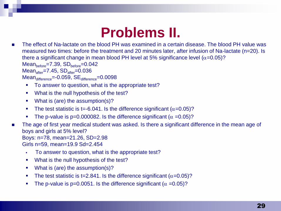
Problems II. The effect of Na-lactate on the blood PH was examined in a certain disease. The blood PH value was

measured two times: before the treatment and 20 minutes later, after infusion of Na-lactate (n=20). Is

there a significant change in mean blood PH level at 5% significance level (=0.05)?

Meanbefore=7.39, SDbefore=0.042

Meanafter=7.45, SDafter=0.036

Meandifference=-0.059, SEdifference=0.0098

To answer to question, what is the appropriate test?

What is the null hypothesis of the test?

What is (are) the assumption(s)?

The test statistic is t=-6.041. Is the difference significant (=0.05)?

The p-value is p=0.000082. Is the difference significant ( =0.05)?

The age of first year medical student was asked. Is there a significant difference in the mean age of

boys and girls at 5% level?

Boys: n=78, mean=21.26, SD=2.98

Girls n=59, mean=19.9 Sd=2.454

To answer to question, what is the appropriate test?

What is the null hypothesis of the test?

What is (are) the assumption(s)?

The test statistic is t=2.841. Is the difference significant (=0.05)?

The p-value is p=0.0051. Is the difference significant ( =0.05)?

29

Documents

Hypothesis tests. One- and two sample t-tests. fileTwo sample t-test (or independent samples t-test). There are two independent samples, coming from two normal populations. We test