Received: 3 May 2018 | Revised: 12 July 2018 | Accepted: 15 July 2018

DOI: 10.1002/gepi.22156

RE S EARCH ART I C L E

Multi‐SKAT: General framework to test for rare‐variantassociation withmultiple phenotypes

Diptavo Dutta1,2 | Laura Scott1,2 | Michael Boehnke1,2 | Seunggeun Lee1,2

1Department of Biostatistics, University ofMichigan, Ann Arbor, Michigan2Center for Statistical Genetics, Universityof Michigan, Ann Arbor, Michigan

CorrespondenceSeunggeun Lee, Department ofBiostatistics, University of Michigan,1420 Washington Heights, Ann Arbor,MI 48105.Email: leeshawn@umich.edu

Funding informationNational Human Genome ResearchInstitute, Grant/Award Numbers: R01HG000376, R01 HG008773; NationalInstitute of Diabetes and Digestive andKidney Diseases, Grant/Award Number:U01 DK062370; U.S. National Library ofMedicine, Grant/Award Number: R01LM012535

Abstract

In genetic association analysis, a joint test of multiple distinct phenotypes can

increase power to identify sets of trait‐associated variants within genes or

regions of interest. Existing multiphenotype tests for rare variants make specific

assumptions about the patterns of association with underlying causal variants,

and the violation of these assumptions can reduce power to detect association.

Here, we develop a general framework for testing pleiotropic effects of rare

variants on multiple continuous phenotypes using multivariate kernel regres-

sion (Multi‐SKAT). Multi‐SKAT models affect sizes of variants on the

phenotypes through a kernel matrix and perform a variance component test

of association. We show that many existing tests are equivalent to specific

choices of kernel matrices with the Multi‐SKAT framework. To increase power

of detecting association across tests with different kernel matrices, we

developed a fast and accurate approximation of the significance of the

minimum observed P value across tests. To account for related individuals,

our framework uses random effects for the kinship matrix. Using simulated data

and amino acid and exome‐array data from the METabolic Syndrome In Men

(METSIM) study, we show that Multi‐SKAT can improve power over single‐phenotype SKAT‐O test and existing multiple‐phenotype tests, while maintain-

ing Type I error rate.

KEYWORD S

Copula, gene‐based test, METSIM study, multiple phenotypes, phenotype kernel, pleiotropy, rare

variants, related individuals, SKAT

1 | INTRODUCTION

Since the advent of array genotyping technologies,genome‐wide association studies (GWASs) have identi-fied numerous genetic variants associated with complextraits. Despite these many discoveries, GWAS loci explainonly a modest proportion of heritability for most traits.This may be due, in part, to the fact that these associationstudies are underpowered to identify associations withrare variants (Korte & Farlow, 2013). To identify suchrare‐variant associations, gene‐ or region‐based multiple

variant tests have been developed (Lee, Abecasis,Boehnke, & Lin, 2014). By jointly testing rare variantsin a target gene or region, these methods can increasepower over a single‐variant test and are now used as astandard approach in rare‐variant analysis.

Recent GWAS results have shown that many GWASloci are associated with multiple traits (Solovieff,Cotsapas, Lee, Purcell, & Smoller, 2013). Nearly, 17% ofvariants in National Heart Lung and Blood Institute(NHLBI) GWAS categories is associated with multipletraits (Sivakumaran et al., 2011). For example, 44% of

Genet. Epidemiol. 2019;43:4–23.www.geneticepi.org4 | © 2018 Wiley Periodicals, Inc.

autoimmune risk single‐nucleotide polymorphisms(SNPs) has been estimated to be associated with two ormore autoimmune diseases (Cotsapas et al., 2011).Detecting such pleiotropic effects is important to under-stand the underlying biological structure of complextraits. In addition, by leveraging cross‐phenotype associa-tions, the power to detect trait‐associated variants can beincreased.

Identifying the cross‐phenotype effects requires asuitable joint or multivariate analysis framework thatcan leverage the dependence of the phenotypes. Variousmethods have been proposed for multiple‐phenotypeanalyses in GWAS (Ferreira & Purcell, 2009; Huang,Johnson, & O’Donnell, 2011; Ray, Pankow, & Basu, 2016;Ried et al., 2012; Zhou & Stephens, 2014). Extendingthem, several groups have developed multiple‐phenotypetests for rare variants (Broadaway et al., 2016; Lee et al.,2016; Maity, Sullivan, & Tzeng, 2012; Sun et al., 2016;Wang et al., 2015; Wu & Pankow, 2016; Yan et al., 2015;Zhan et al., 2017). For example, Wang et al. (2015)proposed a multivariate functional linear model (MFLM);Broadaway et al. (2016) used a dual‐kernel‐baseddistance‐covariance approach to test for cross‐phenotypeeffects of rare variants by comparing similarity inmultivariate phenotypes to similarity in genetic variants(GAMuT; Chiu et al., 2017); Wu and Pankow (2016)developed a score‐based sequence kernel association testfor multiple traits, MSKAT, which has been shown to besimilar in performance to GAMuT (Broadaway et al.,2016); Zhan et al. (2017) proposed a dual kernel basedassociation test (DKAT), which uses the dual‐kernelapproach as in GAMuT but provides more robustperformance when the dimension of phenotypes is highcompared with the sample size.

Despite these developments, existing methods haveimportant limitations. Most methods were developedunder specific assumptions regarding the effects of thevariants on multiple phenotypes, and hence lose power ifthe assumptions are violated (Ray et al., 2016). Forexample, if genetic effects are heterogeneous acrossmultiple phenotypes, methods assuming homogeneousgenetic effects can lose a substantial amount of power.Although there has been a recent attempt to combineanalysis results from different models (Zhan et al., 2017),no scalable methods have been developed to evaluate thesignificance of the combined results in genome‐widescale analysis. In addition, most existing methods andsoftware cannot adjust for relatedness between indivi-duals; thus, to apply these methods, related individualsmust be removed from the analysis to maintain Type Ierror rate. For example, in the METabolic Syndrome InMen (METSIM) study, ~15% of individuals is estimated tobe related up to the second degree.

Here, we develop Multi‐SKAT, a general frameworkthat extends the mixed effect model‐based kernelassociation tests to a multivariate regression frameworkwhile accounting for family relatedness. Mixed effectmodels have been widely used for rare‐variant associa-tion tests. Popular rare‐variant tests, such as SKAT (Wuet al., 2011) and SKAT‐O (Lee, Wu, & Lin, 2012), arebased on mixed effect models. By using kernels to relategenetic variants to multiple continuous phenotypes,Multi‐SKAT allows for flexible modeling of the geneticeffects on the phenotypes. The idea of using kernels forgenotypes and phenotypes was previously used by thedual‐kernel approaches, such as GAMuT and DKAT.However, in contrast to these two similarity‐basedmethods, Multi‐SKAT is multivariate regression basedand hence provides a natural way to adjust for covariatesand also can account for sample relatedness by incorpor-ating random effects for the kinship matrix. Many of theexisting methods for multiple‐phenotype rare‐varianttests can be viewed as special cases of Multi‐SKAT withparticular choices of kernels. Furthermore, to avoid lossof power due to model misspecification, we developcomputationally efficient omnibus tests, which allow foraggregation of tests over several kernels and provide fastP value calculation (Demarta & McNeil, 2005).

The article is organized as follows: In the first section,we present the multivariate mixed effect model andkernel matrices. We particularly focus on the phenotypekernel and describe omnibus procedures that canaggregate results across different choices of kernels andkinship adjustment. In the next section, we describe thesimulation experiments that clearly demonstrate thatMulti‐SKAT tests have increased power to detectassociations compared with existing methods, likeGAMuT, MSKAT, and others in most of the scenarios.Further, we applied Multi‐SKAT to detect the cross‐phenotype effects of rare nonsynonymous and protein‐truncating variants on a set of nine amino acidsmeasured on 8,545 Finnish men from the METSIM study.

2 | MATERIALS AND METHODS

2.1 | Single‐phenotype region‐basedtests

To describe the Multi‐SKAT tests, we first present theexisting model of the single‐phenotype gene or region‐based tests. Let y y y y= ( , ,…, )k k k nk

T1 2 be an n × 1 vector

of the kth phenotype over n individuals; X an n q×matrix of the q nongenetic covariates, including theintercept; G G G= ( ,…, )j j nj

T1 is an n × 1 vector of the

minor allele counts (0, 1, or 2) for a binary genetic variantj; and G G G= [ ,…, ]m1 is an n m× genotype matrix for m

DUTTA ET AL. | 5

genetic variants in a target region. The regression modelshown in Equation (1) can relate m genetic variants tophenotype k:

y Xα Gβ= + + ϵ ,k k k k. (1)

where αk is a q × 1 vector of regression coefficients of qnongenetic covariates, β β β= ( ,…, )k k mk

T. 1 an m × 1 vector

of regression coefficients of the m genetic variants, and ϵkan n × 1 vector of nonsystematic error term with eachelement following N σ(0, )k

2 . To test for βH : = 0k0 . , avariance component test under the mixed effect model hasbeen proposed to increase power over the usual F test (Wuet al., 2011). The variance component test assumes that theregression coefficients, βk. , are random variables and followa centered distribution with variance τ ΣG

2 (see below).Under these assumptions, the test for β = 0k. is equivalentto testing τ = 0. The score statistic for this test is

Q y μ GΣ G y μ= ( − ˆ ) ( − ˆ ),k kT

GT

k k (2)

where μ Xαˆ = ˆk k is the estimated mean of yk under thenull hypothesis of no association. The test statistic Qasymptotically follows a mixture of Χ2 distributionsunder the null hypothesis and P values can be computedby inverting the characteristic function (Davies, 1980).

The kernel matrix ΣG plays a critical role; it models therelationship among the effect sizes of the variants on thephenotypes. Any positive semidefinite matrix can be usedfor ΣG providing a unified framework for the region‐basedtests. A frequent choice of ΣG is a sandwich‐type matrix

WR WΣ =G G , where W w w= diag( , …, )m1 is a diagonalweighting matrix for each variant, and RG is a correlationmatrix between the effect sizes of the variants. R I=G m m×implies uncorrelated effect sizes and corresponds to SKAT,and R = 1 1G m m

T corresponds to the Burden test, whereIm m× is an m m× diagonal matrix and 1 = (1, …, 1)m

T is anm × 1 vector with all elements being unity. Furthermore, alinear combination of these two matrices corresponds toR ρ ρ I= 1 1 + (1 − )G m m

Tm m× , which is used for SKAT‐O

(Lee, Wu et al., 2012).

2.2 | Multiple‐phenotype region‐basedtests

Extending the idea of using kernels, we build a model formultiple phenotypes. The multivariate linear modelshown in Equation (3) can relate genetic variants toK ‐correlated phenotypes:

Y XA GB E= + + , (3)

where Y y y= ( , …, )K1 is an n K× phenotype matrix, A aq K× matrix of coefficients of X , B = β( )ij an m K×matrix of coefficients, where βij denotes the effect of theith variant on the jth phenotype, and E an n K× matrixof nonsystematic errors. Let ⋅vec( ) denote the matrixvectorization function, and then Evec( ) follows

⊗N I V(0, )n , where V is a K K× covariance matrixand ⊗ represents the Kronecker product.

In addition to assuming that βk. follows a centereddistribution with covariance τ ΣG

2 , we further assume thatβ β β= ( , …, )i i iK

T. 1 , which is the vector of regression coeffi-

cients of variant i for K multiple phenotypes, follows acentered distribution with covariance τ ΣP

2 , which impliesthat Bvec( ) follows a centered distribution with covariance

⊗τ Σ ΣG P2 . As before, the null hypothesis BH : vec( ) = 00 isequivalent to τ = 0. The corresponding score test statistic is

⊗

Q Y μ GΣ G

V Σ V Y μ

= vec( ) − vec( ) ( )

( )vec( ) − vec( ),

TG

T

P−1 −1 (4)

where μ and V are the estimated mean and covariance ofY under the null hypothesis.

ΣP plays a similar role as ΣG but with respect tophenotypes. ΣP represents a kernel in the phenotypesspace and models the relationship among the effect sizesof a variant on each of the phenotypes. Any positivesemidefinite matrix can be used as ΣP.

The proposed approach provides a double flexibility inmodeling. Through the choice of structures for ΣG and ΣP,we can control the dependencies of genetic effects.Additionally, similar to SKAT, the use of a sandwich‐type matrix WR WG for ΣG allows us to upweight rarevariants by using β (1, 25) weights as in Wu et al. (2011).Most of our hypotheses about the underlying geneticstructure of a set of phenotypes can be modeled throughvarying structures of these two matrices.

2.3 | Phenotype kernel structure ΣP

The use of ΣG has been extensively studied previously inthe literature (Lee, Emond et al., 2012; Lee, Wu, et al.,2012; Wu et al., 2011). Here, we propose several choicesfor ΣP and study their effect from a modeling perspective.

2.3.1 | Homogeneous (Hom) kernel

It is possible that effect sizes of a variant on differentphenotypes are homogeneous, in which case ⋯β β= =j jK1 .Under this assumption,

Σ = 1 1 .P K KT

,Hom (5)

6 | DUTTA ET AL.

Under ΣP,Hom, the effect sizes β k K, ( = 1, …, )jk for avariant j are the same for all the phenotypes.

2.3.2 | Heterogeneous (Het) kernel

Effect sizes of a variant on different phenotypes can beheterogeneous, in which ≠⋯≠β βj jK1 . Under this as-sumption, we can construct

IΣ = .P k k,Het × (6)

The ΣP,Het implies that the effect sizes (β β, …,j jKT

1 ) areuncorrelated among themselves. This also indicates thatthe correlation among the phenotypes is not affected bythis particular region or gene.

2.3.3 | Phenotype covariance (PhC)kernel

We may model ΣP as proportional to the estimatedresidual covariance across the phenotypes as

VΣ = ,P,PhC (7)

where V is the estimated covariance matrix among thephenotypes. This model assumes that the correlationbetween the effect sizes is proportional to that betweenthe residual phenotypes after adjusting for the nongeneticcovariates.

2.3.4 | Principal component (PC) kernel

Principal component analysis (PCA) is a popular tool formultivariate analysis. In multiple‐phenotype tests,PC‐based approaches have been used to reduce thedimension in phenotypes (Aschard et al., 2014). Here, weshow that PC‐based approach can be included in ourframework. Let L L L= ( , …, )K1 be the loading matrix witheach column Li produces the ith PC score. In AppendixA, we show that using V LV V L VΣ =P P P

T,PC

−1 −1is

equivalent to assuming heterogeneous effects with allPCs as phenotypes. Instead of using all the PCs, we canuse selected PCs that represent the majority of cumula-tive variations in phenotypes. For example, we can jointlytest the PCs that have cumulative variance of 90%. If thetop t PCs have been chosen for analysis using ν%cumulative variance as cutoff, we can use

V L V V L VΣ = ,P ν P PT

,PC− sel−1 −1

sel

where L L L= [ , …, , 0, …, 0]tsel 1 and 0 represents a vectorof 0’s of appropriate length.

2.3.5 | Relationship with othermultiple‐phenotype rare‐variant testsWe have proposed a uniform framework of Multi‐SKATtests that depend on ΣG and ΣP. There are certain specificchoices of kernels that correspond to other publishedmethods.

• Using ΣP,PhC and WI WΣ =G mT is identical to the

GAMuT (Broadaway et al., 2016) with the projectionphenotype kernel and the MSKAT with the Q statistic(Wu & Pankow, 2016).

• Using VΣ =P2 and WI WΣ =G m

T is identical toGAMuT (Broadaway et al., 2016) with the linear

phenotype kernel and the MSKAT with the Q′ statistic(Wu & Pankow, 2016).

• Using ΣP,Hom and WI WΣ =G mT is identical to hom‐

MAAUSS (Lee et al., 2016).• Using ΣP,Het and WI WΣ =G m

T is identical to het‐MAAUSS (Lee et al., 2016) and MF‐KM (Yan et al., 2015).

For the detailed proof, please see Appendix B.

2.4 | Minimum P value‐based omnibustests (minP and minPcom)

The model and the corresponding test of association thatwe propose have two parameters, ΣG and ΣP, which areabsent in the null model of no association. Because ourtest is a score test, ΣG and ΣP cannot be estimated fromthe data. One possible approach is to select ΣG and ΣPbased on prior knowledge; however, if the selected ΣGand ΣP do not reflect underlying biology, the test mayhave substantially reduced power (Lee et al., 2016; Rayet al., 2016). In an attempt to achieve robust power, weaggregate results across different ΣG and ΣP using theminimum of P values from different kernels.

Although this omnibus test approach has been used inrare‐variant tests and multiple‐phenotype analyses forcombining multiple kernels from genotypes and pheno-types (He, Xu, Lee, & Ionita‐Laza, 2017; Urrutia et al.,2015; Wu, Maity, Lee, & Simmons, 2013; Zhan et al.,2017), it is challenging to calculate the P value, becausethe minimum P value does not follow the uniformdistribution. One possible approach is using permutationor perturbation to calculate the Monte‐Carlo P value(Urrutia et al., 2015; Zhan et al., 2017); however, thisapproach is computationally too expensive to be used ingenome‐wide analysis. To address it, here we propose afast Copula‐based P value calculation for Multi‐SKAT,which needs only a small number of resampling steps tocalculate the P value.

DUTTA ET AL. | 7

Suppose ph is the P value for Qh with given hth ΣG andΣP, h b= 1,…, , and T p p= ( , …, )P b

T1 is a b × 1 vector of

P values of b such Multi‐SKAT tests. The minimumP value test statistic after the Bonferroni adjustment isb × pmin, where pmin is the minimum of the b P values. Inthe presence of positive correlation among the tests, thisapproach is conservative and hence might lack power ofdetection. Rather than using the Bonferroni‐correctedpmin, more accurate results can be obtained if the jointnull distribution or more specifically the correlationstructure of TP can be estimated. Here, we adopt aresampling‐based approach to estimate this correlationstructure. Note that our test statistic is equivalent to

⎜ ⎟⎧⎨⎩

⎛⎝

⎞⎠

⎫⎬⎭⊗Q S G G V V S= ( Σ ) Σ ,TG

TP

− 12 − 1

2 (8)

where ⊗S I V Y μ= ( )vec( ) − vec( )n− 1

2 . Under the nullhypothesis, S approximately follows an uncorrelatednormal distribution N I(0, )nK . Using this, we proposethe following resampling algorithm:

1. Generate nK samples from an N (0, 1) distribution,say SR.

2. Calculate b different test statistics as Q S=R RT

⊗G G V V S( Σ ) ( Σ )GT

P R− −1

212 for all the choices of ΣP

and calculate P values.3. Repeat the previous steps independently for

R (=1,000) iterations and calculate the correlationbetween the P values of the tests from the Rresampling P values.

With the estimated null‐correlation structure, we usea Copula to approximate the joint distribution of TP(Demarta & McNeil, 2005; He et al., 2017). Copula is astatistical approach to construct joint multivariatedistribution using marginal distribution of each variableand correlation structure. Because marginally each teststatistic Q follows a mixture of Χ2 distributions, whichhas a heavier tail than normal distribution, we propose touse a t‐Copula to approximate the joint distribution, thatis, we assume the joint distribution of TP to be multi-variate t with the estimated correlation structure. Thefinal P value for association is then calculated from thedistribution function of the assumed t‐Copula.

When calculating the correlation across the P values,Pearson’s correlation coefficient can be unreliable be-cause it depends on normality and homoscedasticityassumptions. To avoid such assumptions, we recommendestimating the null‐correlation matrix of the P valuesthrough Kendall’s tau τ( ), which is a nonparametricapproach based on concordance of ranks.

The minimum P value approach can be used tocombine different ΣP’s given ΣG, or combine both ΣP andΣG. For example, two ΣG’s corresponding to SKAT (WW )and Burden kernels (W W1 1m m

T ) and four ΣP’s (ΣP,Hom,ΣP,Het, ΣP,PhC, and ΣP,PC−0.9) can be combined, whichresults in the omnibus test of these eight different tests.To differentiate the latter, we will call it minPcom, whichcombines SKAT and Burden‐type kernels of ΣG.

2.5 | Adjusting for relatedness

We formulated Equation (3) and corresponding testsunder the assumption of independent individuals. Ifindividuals are related, this assumption is no longer valid,and the tests may have inflated Type I error rate. Becauseour method is regression based, we can relax theindependence assumption by introducing a random effectterm to account for the relatedness among individuals.

Let Φ be the kinship matrix of the individuals andVg isa coheritability matrix, denoting the shared heritabilitybetween the phenotypes. Extending the model presentedin Equation (3), we incorporate Φ and Vg as

Y XA GB Z E= + + + , (9)

where Z is an n K× matrix with Zvec( ) following⊗N Φ V(0, )g . Z represents a matrix of random effects

arising from shared genetic effects between individualsdue to the relatedness. The remaining terms are the sameas in Equation (3). The corresponding score teststatistic is

⊗∕ ∕Q S V G G V S= ( Σ ) Σ ,K K

TG

TP Kin in e

−1 2e−1 2

in (10)

where ∕S V Y μ= vec( ) − vec( )K in e−1 2

and ⊗V Φ=e ⊗V I V+g n is the estimated covariance matrix of Yvec( )under the null hypothesis. Similar to the previous versionsfor unrelated individuals, QK in asymptotically follows amixture of Χ2 under the assumption of no association.

This approach depends on the estimation of the matricesΦ, Vg, and V . The kinship matrix Φ can be estimatedusing the genome‐wide genotype data (Manichaikul et al.,2010). Several of the published methods, like LD‐Score(Bulik‐Sullivan et al., 2015), phenotype imputation expedited(PHENIX) (Dahl et al., 2016), and genome-wide efficientmixed model association (GEMMA) (Zhou & Stephens,2014; Zhou, Carbonetto, & Matthew, 2013) can jointlyestimate Vg and V . In our numerical analysis, we have usedPHENIX. This is an efficient method to fit local maximumlikelihood variance components in a multiple‐phenotype‐mixed model through an E–M algorithm.

Once the matrices Φ, Vg, and V are estimated, wecompute the asymptotic P values for QK in by using a

8 | DUTTA ET AL.

mixture of Χ2 distribution. The computation of QK inrequires large matrix multiplications, which can be timeand memory consuming. To reduce computationalBurden, we employ several transformations. We performan eigen decomposition on the kinship matrix Φ asΦ UΛU= T , where U is an orthogonal matrix ofeigenvectors and Λ is a diagonal matrix of correspondingeigenvalues. We obtain the transformed phenotypematrix as

∼Y U′Y= , the transformed covariate matrix as∼X U′X= , the transformed random effects matrix∼Z U′Z= and transformed residual error matrix∼E U′E= . Equation (9) can be transformed into

⊗

⊗

∼ ∼ ∼ ∼

∼

∼ ∼Y X A GB Z E Z N Λ V

E N I V

= + + + , vec( ) ~ (0, ),

vec( ) ~ (0, ).

g

(11)

All the properties of the tests developed from Equation (3)are directly applicable to those from Equation (11).QK in canbe computed from this transformed equation as

⊗ ∼ ∼∼ ∼∕ ∕Q S V G G V S= ( Σ ) Σ ,K KT

GT

P Kin in e−1 2

e−1 2

in (12)

where ∼ ∼∼ ∕S V Y μ= vec( ) − vec( )K in e−1 2

, ∼μ is the estimatedmean of

∼Y under the null hypothesis and ⊗ ⊗

∼V Λ V I V= +g ne . Asymptotic P values can beobtained from the corresponding mixture of Χ2 distribu-tion. Further, omnibus strategies for the tests developedfrom Equation (3) are applicable in this case with similarmodifications. For example, the resampling algorithm forminimum P value‐based omnibus test can be implemen-ted here as well by noting that SK in approximately followsan uncorrelated normal distribution.

3 | SIMULATIONS

We carried out extensive simulation studies to evaluate theType I error control and power of Multi‐SKAT tests. ForType I error simulations without related individuals and allpower simulations, we generated 10,000 chromosomes over1Mbp regions using a coalescent simulator with theEuropean demographic model (Schaffner et al., 2005). Theminor allele frequency (MAF) spectrum of the simulatedvariants is shown in Supporting Information Figure S6,showing that most of the variants are rare variants. Becausethe average length of the gene is 3 kbps, we randomlyselected a 3‐kbps region for each simulated data set to testfor associations. For the Type I error simulations withrelated individuals, to have a realistic kinship structure, weused the METSIM study genotype data.

Phenotypes were generated from the multivariatenormal distribution as

⋯y β G β G I V~ MVN( + + ) , ,i m m1 1 (13)

where y y y= ( ,…, )i i iKT

1 is the outcome vector, Gj thegenotype of the jth variant, and βj the correspondingeffect size, and V a covariance of the nonsystematic errorterm. We use V to define level of covariance between thetraits. I is a k × 1 indicator vector, which has 1 when thecorresponding phenotype is associated with the regionand 0 otherwise. For example, if there are fivephenotypes and the last three are associated with theregion, I = (0, 0, 1, 1, 1)T .

To evaluate whether Multi‐SKAT can control Type I errorunder realistic scenarios, we simulated a data set with ninephenotypes with a correlation structure identical to that ofnine amino acid phenotypes in the METSIM data (seeSupporting Information Figure S1). Phenotypes were gener-ated using Equation (13) with β = 0. Total 5,000,000 datasets with 5,000 individuals were generated to obtain theempirical Type I error rates at α = 10 , 10−4 −5, and2.5 × 10−6, which are corresponding to candidate genestudies to test for 500 and 5,000 genes and exome‐widestudies to test for all 20,000 protein coding genes,respectively.

Next, we evaluated Type I error controls in the presenceof related individuals. To have a realistic related structure, weused the METSIM study genotype data. We generated arandom subsample of 5,000 individuals from theMETSIM study individuals and generated null values forthe nine phenotypes from VMVN(0, ),e where

⊗ ⊗V Φ V I V= +ge 5k ;5k 5k, Φ5k is the estimated kinshipmatrix of the 5,000 selected individuals, Vg;5k and V5k areestimated coheritability and residual variance matrices,respectively, for these individuals as estimated using themultiple phenotype mixed model (MPMM) function in thePHENIX R‐package (version 1.0 See Web Resources). Foreach set of nine phenotypes, we performed the Multi‐SKATtests for randomly selected 5,000 genes in the METSIM data.For the details about the data, see the next section. Wecarried out this procedure 1,000 times and obtained5, 000, 000 P values and estimated Type I error rate asproportions of P values smaller than the given level α.

Our simulation studies focus on evaluating the power ofthe proposed tests when the number of phenotypes is five orsix. Power simulations were performed both in situationswhen there was no pleiotropy (i.e., only one of thephenotypes was associated with the causal variants) andalso when there was pleiotropy. Under pleiotropy, because itis unlikely that all the phenotypes are associated withgenotypes in the region, we varied the number of phenotypesassociated. For each associated phenotype, 30% or 50% of therare variants (MAF< 1%) was randomly selected to becausal variants. We modeled the rarer variants to havestronger effect, as ∣ ∣ ∣ ∣β c= log (MAF )j j10 . We used c = 0.3,

DUTTA ET AL. | 9

which yields ∣ ∣β = 0.9j for variants with MAF= 10−3. Ourchoice of β yielded the average heritability of associatedphenotypes between 1% and 4%. We also consideredsituations that all causal variants were trait‐increasingvariants (i.e., positive β) or 20% of causal variants wastrait‐decreasing variants (i.e., negative β). Empirical powerwas estimated from 1,000 independent data sets at exome‐wide α = 2.5 × 10−6.

In Type I error and power simulations, we comparedthe following tests:

• Bonferroni‐adjusted minimum P values from gene‐based test (SKAT, Burden, or SKAT‐O) on eachphenotype (minPhen),

• Multi‐SKAT with ΣP,Hom (Hom),• Multi‐SKAT with ΣP,Het (Het),• Multi‐SKAT with ΣP,PhC (PhC),• Multi‐SKAT with ΣP,PC−0.9 (PC‐Sel),• Minimum P value of Hom, Het, PhC, and PC‐Sel usingCopula (minP),

• Minimum P value of Hom, Het, PhC, and PC‐Sel withΣG being SKAT and Burden, using Copula (minPcom).

For the Multi‐SKAT tests, we used two different ΣG’scorresponding to SKAT (i.e., WWΣ =G ) and Burden tests(i.e., W WΣ = 1 1G m m

T ). For the variant weighting matrixW w w= diag( ,…, )m1 , we used w β= (MAF , 1, 25)j j func-tion to upweight rarer variants, as recommended by Wuet al. (2011).

3.1 | Computation time

We estimated the computation time of Multi‐SKAT tests andthe existing methods. Using simulated data sets of 5,000related and unrelated individuals with 10 phenotypes and 20genetic variants, we estimated the computation time ofMulti‐SKAT tests with and without kinship adjustments. Tocompare the computation performance of Multi‐SKAT testswith the existing methods, we generated data sets ofunrelated individuals with five different sample sizes(n=1,000, 2,000, 10,000, 15,000, and 20,000) and fourdifferent number of variants (m = 10, 20, 50, and 100).For each simulation setup, we generated 100 data sets andobtained the average value of the computation time.

3.2 | Analysis of the METSIM studyExomeChip data

To investigate the cross‐phenotype roles of low frequencyand rare variants on amino acids, we analyzed data on8,545 participants of the METSIM study on whom allnine amino acids (alanine, leucine, isoleucine, glycine,valine, tyrosine, phenylalanine, glutamine, and histidine)were measured by proton nuclear magnetic resonance

spectroscopy (Teslovich et al., 2018). Individuals weregenotyped on the Illumina ExomeChip and OmniExpressarrays, and we included individuals that passed samplequality control filters (Huyghe et al., 2013). The kinshipbetween the individuals was estimated via KING (version2.0; Manichaikul et al., 2010, See Web Resources). Weadjusted the amino acid levels for age, age2, and BMI andinverse normalized the residuals. The phenotype correla-tion matrix after covariate adjustment is shown in Figure3 and Supporting Information Figure S1. Subsequently,we estimated the genetic heritability matrix and theresidual covariance matrix using the MPMM functionfrom PHENIX R‐package (Dahl et al., 2016).

We included rare (MAF< 1%) nonsynonymous andprotein‐truncating variants with a total rare minor allelecount of at least five for genes that had at least three rarevariants leaving 5,207 genes for analysis. We set astringent significance threshold at 9.6 × 10−6 correspond-ing to the Bonferroni adjustment for 5,207 genes. Further,we also considered a less stringent threshold of 10−4,corresponding to a candidate gene study of 500 genes, assuggestive to study the associations, which were notsignificant but close to the threshold.

4 | RESULTS

4.1 | Type I error simulations

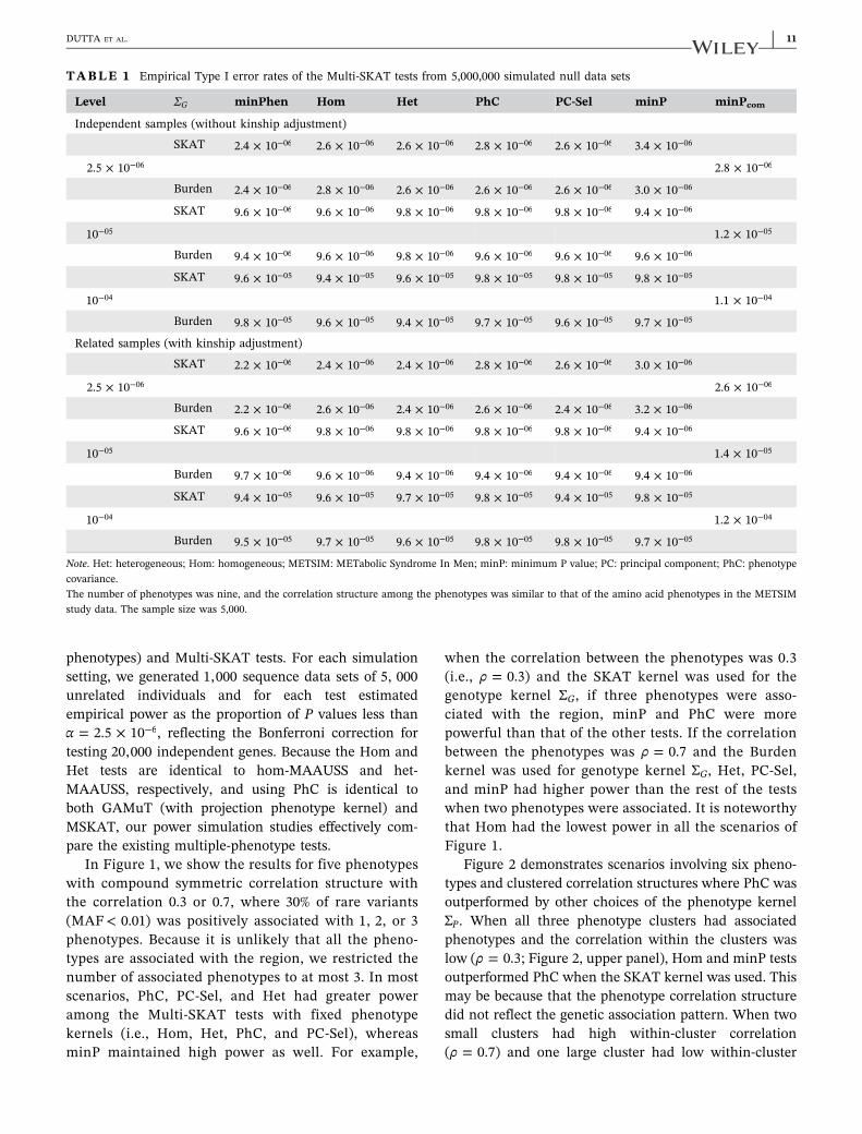
We estimated empirical Type I error rates of the Multi‐SKAT tests with and without related individuals. Forunrelated individuals, we simulated 5,000 individualsand nine phenotypes based on the correlation structurefor the amino acid phenotypes in the METSIM studydata. For related individuals, we simulated 5,000individuals using the kinship matrix for randomlychosen METSIM individuals (see Section 2). Weperformed association tests and estimated Type I errorrate as the proportion of P values less than the specifiedα levels. Type I error rates of the Multi‐SKAT tests werewell maintained at α = 10 , 10−4 −5, and 2.5 × 10−6 forboth unrelated and related individuals (Table 1), whichcorrespond to candidate gene studies of 500 and5,000 genes and exome‐wide studies to test for all20,000 protein coding genes, respectively. For example,at level α = 2.5 × 10−6, the largest empirical Type Ierror rate from any of the Multi‐SKAT tests was3.4 × 10−6, which was within the 95% confidenceinterval (CI = [1.6 × 10−6, 4 × 10−6]).

4.2 | Power simulations

We compared the empirical power of the minPhen(Bonferroni‐adjusted minimum P value for the

10 | DUTTA ET AL.

phenotypes) and Multi‐SKAT tests. For each simulationsetting, we generated 1,000 sequence data sets of 5, 000unrelated individuals and for each test estimatedempirical power as the proportion of P values less thanα = 2.5 × 10−6, reflecting the Bonferroni correction fortesting 20,000 independent genes. Because the Hom andHet tests are identical to hom‐MAAUSS and het‐MAAUSS, respectively, and using PhC is identical toboth GAMuT (with projection phenotype kernel) andMSKAT, our power simulation studies effectively com-pare the existing multiple‐phenotype tests.

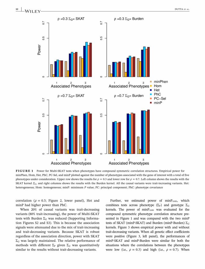
In Figure 1, we show the results for five phenotypeswith compound symmetric correlation structure withthe correlation 0.3 or 0.7, where 30% of rare variants(MAF< 0.01) was positively associated with 1, 2, or 3phenotypes. Because it is unlikely that all the pheno-types are associated with the region, we restricted thenumber of associated phenotypes to at most 3. In mostscenarios, PhC, PC‐Sel, and Het had greater poweramong the Multi‐SKAT tests with fixed phenotypekernels (i.e., Hom, Het, PhC, and PC‐Sel), whereasminP maintained high power as well. For example,

when the correlation between the phenotypes was 0.3(i.e., ρ = 0.3) and the SKAT kernel was used for thegenotype kernel ΣG, if three phenotypes were asso-ciated with the region, minP and PhC were morepowerful than that of the other tests. If the correlationbetween the phenotypes was ρ = 0.7 and the Burdenkernel was used for genotype kernel ΣG, Het, PC‐Sel,and minP had higher power than the rest of the testswhen two phenotypes were associated. It is noteworthythat Hom had the lowest power in all the scenarios ofFigure 1.

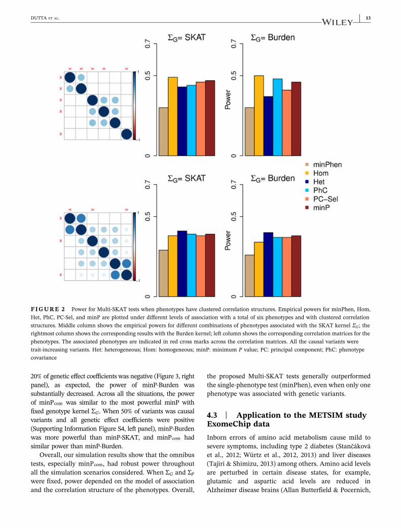
Figure 2 demonstrates scenarios involving six pheno-types and clustered correlation structures where PhC wasoutperformed by other choices of the phenotype kernelΣP. When all three phenotype clusters had associatedphenotypes and the correlation within the clusters waslow (ρ = 0.3; Figure 2, upper panel), Hom and minP testsoutperformed PhC when the SKAT kernel was used. Thismay be because that the phenotype correlation structuredid not reflect the genetic association pattern. When twosmall clusters had high within‐cluster correlation(ρ = 0.7) and one large cluster had low within‐cluster

TABLE 1 Empirical Type I error rates of the Multi‐SKAT tests from 5,000,000 simulated null data sets

Level ΣG minPhen Hom Het PhC PC‐Sel minP minPcom

Independent samples (without kinship adjustment)

SKAT 2.4 × 10−06 2.6 × 10−06 2.6 × 10−06 2.8 × 10−06 2.6 × 10−06 3.4 × 10−06

2.5 × 10−06 2.8 × 10−06

Burden 2.4 × 10−06 2.8 × 10−06 2.6 × 10−06 2.6 × 10−06 2.6 × 10−06 3.0 × 10−06

SKAT 9.6 × 10−06 9.6 × 10−06 9.8 × 10−06 9.8 × 10−06 9.8 × 10−06 9.4 × 10−06

10−05 1.2 × 10−05

Burden 9.4 × 10−06 9.6 × 10−06 9.8 × 10−06 9.6 × 10−06 9.6 × 10−06 9.6 × 10−06

SKAT 9.6 × 10−05 9.4 × 10−05 9.6 × 10−05 9.8 × 10−05 9.8 × 10−05 9.8 × 10−05

10−04 1.1 × 10−04

Burden 9.8 × 10−05 9.6 × 10−05 9.4 × 10−05 9.7 × 10−05 9.6 × 10−05 9.7 × 10−05

Related samples (with kinship adjustment)

SKAT 2.2 × 10−06 2.4 × 10−06 2.4 × 10−06 2.8 × 10−06 2.6 × 10−06 3.0 × 10−06

2.5 × 10−06 2.6 × 10−06

Burden 2.2 × 10−06 2.6 × 10−06 2.4 × 10−06 2.6 × 10−06 2.4 × 10−06 3.2 × 10−06

SKAT 9.6 × 10−06 9.8 × 10−06 9.8 × 10−06 9.8 × 10−06 9.8 × 10−06 9.4 × 10−06

10−05 1.4 × 10−05

Burden 9.7 × 10−06 9.6 × 10−06 9.4 × 10−06 9.4 × 10−06 9.4 × 10−06 9.4 × 10−06

SKAT 9.4 × 10−05 9.6 × 10−05 9.7 × 10−05 9.8 × 10−05 9.4 × 10−05 9.8 × 10−05

10−04 1.2 × 10−04

Burden 9.5 × 10−05 9.7 × 10−05 9.6 × 10−05 9.8 × 10−05 9.8 × 10−05 9.7 × 10−05

Note. Het: heterogeneous; Hom: homogeneous; METSIM: METabolic Syndrome In Men; minP: minimum P value; PC: principal component; PhC: phenotypecovariance.The number of phenotypes was nine, and the correlation structure among the phenotypes was similar to that of the amino acid phenotypes in the METSIMstudy data. The sample size was 5,000.

DUTTA ET AL. | 11

correlation (ρ = 0.3; Figure 2, lower panel), Het andminP had higher power than PhC.

When 20% of causal variants was trait‐decreasingvariants (80% trait‐increasing), the power of Multi‐SKATtests with Burden ΣG was reduced (Supporting Informa-tion Figures S2 and S3). This is because the associationsignals were attenuated due to the mix of trait‐increasingand trait‐decreasing variants. Because SKAT is robustregardless of the association direction, power with SKATΣG was largely maintained. The relative performance ofmethods with different ΣP given ΣG was quantitativelysimilar to the results without trait‐decreasing variants.

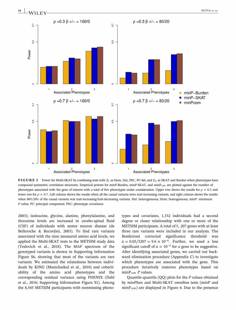
Further, we estimated power of minPcom, whichcombines tests across phenotype (ΣP) and genotype ΣGkernels. The power of minPcom was evaluated for thecompound symmetric phenotype correlation structure pre-sented in Figure 1 and was compared with the two minPtests of SKAT (minP‐SKAT) and Burden (minP‐Burden) ΣGkernels. Figure 3 shows empirical power with and withouttrait‐decreasing variants. When all genetic effect coefficientswere positive (Figure 3, left panel), the performances ofminP‐SKAT and minP‐Burden were similar for both thesituations where the correlations between the phenotypeswere low (i.e., ρ = 0.3) and high (i.e., ρ = 0.7). When

FIGURE 1 Power for Multi‐SKAT tests when phenotypes have compound symmetric correlation structures. Empirical power forminPhen, Hom, Het, PhC, PC‐Sel, and minP plotted against the number of phenotypes associated with the gene of interest with a total of fivephenotypes under consideration. Upper row shows the results for ρ = 0.3 and lower row for ρ = 0.7. Left column shows the results with theSKAT kernel ΣG, and right columns shows the results with the Burden kernel. All the causal variants were trait‐increasing variants. Het:heterogeneous; Hom: homogeneous; minP: minimum P value; PC: principal component; PhC: phenotype covariance

12 | DUTTA ET AL.

20% of genetic effect coefficients was negative (Figure 3, rightpanel), as expected, the power of minP‐Burden wassubstantially decreased. Across all the situations, the powerof minPcom was similar to the most powerful minP withfixed genotype kernel ΣG. When 50% of variants was causalvariants and all genetic effect coefficients were positive(Supporting Information Figure S4, left panel), minP‐Burdenwas more powerful than minP‐SKAT, and minPcom hadsimilar power than minP‐Burden.

Overall, our simulation results show that the omnibustests, especially minPcom, had robust power throughoutall the simulation scenarios considered. When ΣG and ΣPwere fixed, power depended on the model of associationand the correlation structure of the phenotypes. Overall,

the proposed Multi‐SKAT tests generally outperformedthe single‐phenotype test (minPhen), even when only onephenotype was associated with genetic variants.

4.3 | Application to the METSIM studyExomeChip data

Inborn errors of amino acid metabolism cause mild tosevere symptoms, including type 2 diabetes (Stančákováet al., 2012; Würtz et al., 2012, 2013) and liver diseases(Tajiri & Shimizu, 2013) among others. Amino acid levelsare perturbed in certain disease states, for example,glutamic and aspartic acid levels are reduced inAlzheimer disease brains (Allan Butterfield & Pocernich,

FIGURE 2 Power for Multi‐SKAT tests when phenotypes have clustered correlation structures. Empirical powers for minPhen, Hom,Het, PhC, PC‐Sel, and minP are plotted under different levels of association with a total of six phenotypes and with clustered correlationstructures. Middle column shows the empirical powers for different combinations of phenotypes associated with the SKAT kernel ΣG; therightmost column shows the corresponding results with the Burden kernel; left column shows the corresponding correlation matrices for thephenotypes. The associated phenotypes are indicated in red cross marks across the correlation matrices. All the causal variants weretrait‐increasing variants. Het: heterogeneous; Hom: homogeneous; minP: minimum P value; PC: principal component; PhC: phenotypecovariance

DUTTA ET AL. | 13

2003); isoleucine, glycine, alanine, phenylalanine, andthreonine levels are increased in cerebo‐spinal fluid(CSF) of individuals with motor neuron disease (deBelleroche & Recordati, 2003). To find rare variantsassociated with the nine measured amino acid levels, weapplied the Multi‐SKAT tests to the METSIM study data(Teslovich et al., 2018). The MAF spectrum of thegenotyped variants is shown in Supporting InformationFigure S6, showing that most of the variants are rarevariants. We estimated the relatedness between indivi-duals by KING (Manichaikul et al., 2010) and coherit-ability of the amino acid phenotypes and thecorresponding residual variance using PHENIX (Dahlet al., 2016; Supporting Information Figure S1). Amongthe 8,545 METSIM participants with nonmissing pheno-

types and covariates, 1,332 individuals had a seconddegree or closer relationship with one or more of theMETSIM participants. A total of 5, 207 genes with at leastthree rare variants were included in our analysis. TheBonferroni corrected significance threshold was

∕α = 0.05 5207 = 9.6 × 10−6. Further, we used a lesssignificant cutoff of α = 10−4 for a gene to be suggestive.After identifying associated genes, we carried out back-ward elimination procedure (Appendix C) to investigatewhich phenotypes are associated with the gene. Thisprocedure iteratively removes phenotypes based onminPcom P values.

Quantile‐quantile (QQ) plots for the P values obtainedby minPhen and Multi‐SKAT omnibus tests (minP andminPcom) are displayed in Figure 4. Due to the presence

FIGURE 3 Power for Multi‐SKAT by combining tests with ΣP as Hom, Het, PhC, PC‐Sel, and ΣG as SKAT and Burden when phenotypes havecompound symmetric correlation structures. Empirical powers for minP‐Burden, minP‐SKAT, and minPcom are plotted against the number ofphenotypes associated with the gene of interest with a total of five phenotypes under consideration. Upper row shows the results for ρ = 0.3 andlower row for ρ = 0.7. Left column shows the results when all the causal variants were trait‐increasing variants, and right column shows the resultswhen 80%/20% of the causal variants was trait‐increasing/trait‐decreasing variants. Het: heterogeneous; Hom: homogeneous; minP: minimumP value; PC: principal component; PhC: phenotype covariance

14 | DUTTA ET AL.

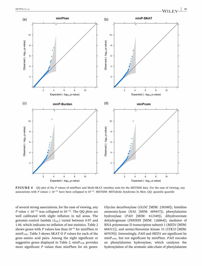
of several strong associations, for the ease of viewing, anyP value < 10−12 was collapsed to 10−12. The QQ plots arewell calibrated with slight inflation in tail areas. Thegenomic‐control lambda (λGC) varied between 0.97 and1.04, which indicates no inflation of test statistics. Table 2shows genes with P values less than 10−4 for minPhen orminPcom. Table 5 shows SKAT‐O P values for each of thegene–amino acid pairs. Among the eight significant orsuggestive genes displayed in Table 2, minPcom providesmore significant P values than minPhen for six genes:

Glycine decarboxylase (GLDC [MIM: 238300]), histidineammonia‐lyase (HAL [MIM: 609457]), phenylalaninehydroxylase (PAH [MIM: 612349]), dihydroorotatedehydrogenase (DHODH [MIM: 126064]), mediator ofRNA polymerase II transcription subunit 1 (MED1 [MIM:604311]), and serine/threonine kinase 33 (STK33 [MIM:607670]). Interestingly, PAH and MED1 are significant byminPcom, but not significant by minPhen. PAH encodesan phenylalanine hydroxylase, which catalyzes thehydroxylation of the aromatic side‐chain of phenylalanine

FIGURE 4 QQ plot of the P values of minPhen and Multi‐SKAT omnibus tests for the METSIM data. For the ease of viewing, anyassociations with P values < 10−12 have been collapsed to 10−12. METSIM: METabolic Syndrome In Men; QQ: quantile quantile

DUTTA ET AL. | 15

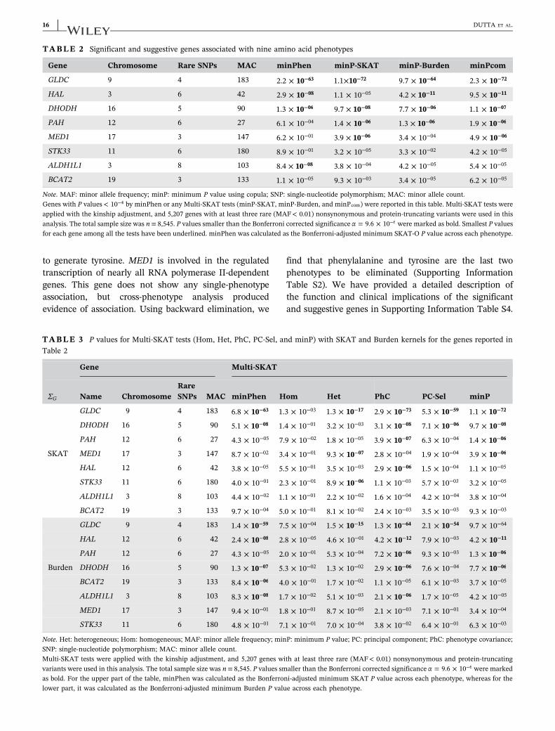
to generate tyrosine. MED1 is involved in the regulatedtranscription of nearly all RNA polymerase II‐dependentgenes. This gene does not show any single‐phenotypeassociation, but cross‐phenotype analysis producedevidence of association. Using backward elimination, we

find that phenylalanine and tyrosine are the last twophenotypes to be eliminated (Supporting InformationTable S2). We have provided a detailed description ofthe function and clinical implications of the significantand suggestive genes in Supporting Information Table S4.

TABLE 2 Significant and suggestive genes associated with nine amino acid phenotypes

Gene Chromosome Rare SNPs MAC minPhen minP‐SKAT minP‐Burden minPcom

GLDC 9 4 183 102.2 × 63− 101.1× 72− 109.7 × 64− 102.3 × 72−

HAL 3 6 42 102.9 × 08− 1.1 × 10−05 104.2 × 11− 109.5 × 11−

DHODH 16 5 90 101.3 × 06− 109.7 × 08− 107.7 × 06− 101.1 × 07−

PAH 12 6 27 6.1 × 10−04 101.4 × 06− 101.3 × 06− 101.9 × 06−

MED1 17 3 147 6.2 × 10−01 103.9 × 06− 3.4 × 10−04 104.9 × 06−

STK33 11 6 180 8.9 × 10−01 3.2 × 10−05 3.3 × 10−02 4.2 × 10−05

ALDH1L1 3 8 103 108.4 × 08− 3.8 × 10−04 4.2 × 10−05 5.4 × 10−05

BCAT2 19 3 133 1.1 × 10−05 9.3 × 10−03 3.4 × 10−05 6.2 × 10−05

Note. MAF: minor allele frequency; minP: minimum P value using copula; SNP: single‐nucleotide polymorphism; MAC: minor allele count.Genes with P values < 10−4 by minPhen or any Multi‐SKAT tests (minP‐SKAT, minP‐Burden, and minPcom) were reported in this table. Multi‐SKAT tests wereapplied with the kinship adjustment, and 5,207 genes with at least three rare (MAF< 0.01) nonsynonymous and protein‐truncating variants were used in thisanalysis. The total sample size was n= 8,545. P values smaller than the Bonferroni corrected significance α = 9.6 × 10−6 were marked as bold. Smallest P valuesfor each gene among all the tests have been underlined. minPhen was calculated as the Bonferroni‐adjusted minimum SKAT‐O P value across each phenotype.

TABLE 3 P values for Multi‐SKAT tests (Hom, Het, PhC, PC‐Sel, and minP) with SKAT and Burden kernels for the genes reported inTable 2

Gene Multi‐SKAT

ΣG Name ChromosomeRareSNPs MAC minPhen Hom Het PhC PC‐Sel minP

GLDC 9 4 183 106.8 × 63− 1.3 × 10−03 101.3 × 17− 102.9 × 73− 105.3 × 59− 101.1 × 72−

DHODH 16 5 90 105.1 × 08− 1.4 × 10−01 3.2 × 10−03 103.1 × 08− 107.1 × 06− 109.7 × 08−

PAH 12 6 27 4.3 × 10−05 7.9 × 10−02 1.8 × 10−05 103.9 × 07− 6.3 × 10−04 101.4 × 06−

SKAT MED1 17 3 147 8.7 × 10−02 3.4 × 10−01 109.3 × 07− 2.8 × 10−04 1.9 × 10−04 103.9 × 06−

HAL 12 6 42 3.8 × 10−05 5.5 × 10−01 3.5 × 10−03 102.9 × 06− 1.5 × 10−04 1.1 × 10−05

STK33 11 6 180 4.0 × 10−01 2.3 × 10−01 108.9 × 06− 1.1 × 10−03 5.7 × 10−03 3.2 × 10−05

ALDH1L1 3 8 103 4.4 × 10−02 1.1 × 10−01 2.2 × 10−02 1.6 × 10−04 4.2 × 10−04 3.8 × 10−04

BCAT2 19 3 133 9.7 × 10−04 5.0 × 10−01 8.1 × 10−02 2.4 × 10−03 3.5 × 10−03 9.3 × 10−03

GLDC 9 4 183 101.4 × 59− 7.5 × 10−04 101.5 × 15− 101.3 × 64− 102.1 × 54− 9.7 × 10−64

HAL 12 6 42 102.4 × 08− 2.8 × 10−05 4.6 × 10−01 104.2 × 12− 7.9 × 10−03 104.2 × 11−

PAH 12 6 27 4.3 × 10−05 2.0 × 10−01 5.3 × 10−04 107.2 × 06− 9.3 × 10−03 101.3 × 06−

Burden DHODH 16 5 90 101.3 × 07− 5.3 × 10−02 1.3 × 10−02 102.9 × 06− 7.6 × 10−04 107.7 × 06−

BCAT2 19 3 133 108.4 × 06− 4.0 × 10−01 1.7 × 10−02 1.1 × 10−05 6.1 × 10−03 3.7 × 10−05

ALDH1L1 3 8 103 108.3 × 08− 1.7 × 10−02 5.1 × 10−03 102.1 × 06− 1.7 × 10−05 4.2 × 10−05

MED1 17 3 147 9.4 × 10−01 1.8 × 10−01 8.7 × 10−05 2.1 × 10−03 7.1 × 10−01 3.4 × 10−04

STK33 11 6 180 4.8 × 10−01 7.1 × 10−01 7.0 × 10−04 3.8 × 10−02 6.4 × 10−01 6.3 × 10−03

Note. Het: heterogeneous; Hom: homogeneous; MAF: minor allele frequency; minP: minimum P value; PC: principal component; PhC: phenotype covariance;SNP: single‐nucleotide polymorphism; MAC: minor allele count.Multi‐SKAT tests were applied with the kinship adjustment, and 5,207 genes with at least three rare (MAF< 0.01) nonsynonymous and protein‐truncatingvariants were used in this analysis. The total sample size was n= 8,545. P values smaller than the Bonferroni corrected significance α = 9.6 × 10−6 were markedas bold. For the upper part of the table, minPhen was calculated as the Bonferroni‐adjusted minimum SKAT P value across each phenotype, whereas for thelower part, it was calculated as the Bonferroni‐adjusted minimum Burden P value across each phenotype.

16 | DUTTA ET AL.

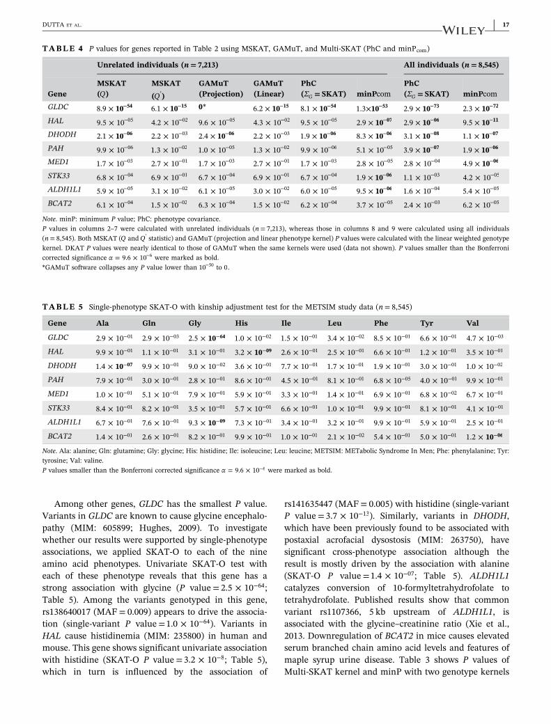
Among other genes, GLDC has the smallest P value.Variants in GLDC are known to cause glycine encephalo-pathy (MIM: 605899; Hughes, 2009). To investigatewhether our results were supported by single‐phenotypeassociations, we applied SKAT‐O to each of the nineamino acid phenotypes. Univariate SKAT‐O test witheach of these phenotype reveals that this gene has astrong association with glycine (P value = 2.5 × 10−64;Table 5). Among the variants genotyped in this gene,rs138640017 (MAF= 0.009) appears to drive the associa-tion (single‐variant P value =1.0 × 10−64). Variants inHAL cause histidinemia (MIM: 235800) in human andmouse. This gene shows significant univariate associationwith histidine (SKAT‐O P value =3.2 × 10−8; Table 5),which in turn is influenced by the association of

rs141635447 (MAF= 0.005) with histidine (single‐variantP value =3.7 × 10−13). Similarly, variants in DHODH,which have been previously found to be associated withpostaxial acrofacial dysostosis (MIM: 263750), havesignificant cross‐phenotype association although theresult is mostly driven by the association with alanine(SKAT‐O P value =1.4 × 10−07; Table 5). ALDH1L1catalyzes conversion of 10‐formyltetrahydrofolate totetrahydrofolate. Published results show that commonvariant rs1107366, 5 kb upstream of ALDH1L1, isassociated with the glycine–creatinine ratio (Xie et al.,2013. Downregulation of BCAT2 in mice causes elevatedserum branched chain amino acid levels and features ofmaple syrup urine disease. Table 3 shows P values ofMulti‐SKAT kernel and minP with two genotype kernels

TABLE 4 P values for genes reported in Table 2 using MSKAT, GAMuT, and Multi‐SKAT (PhC and minPcom)

Unrelated individuals (n= 7,213) All individuals (n= 8,545)

MSKAT MSKAT GAMuT GAMuT PhC PhCGene (Q) (Q′) (Projection) (Linear) (ΣG = SKAT) minPcom (ΣG = SKAT) minPcomGLDC 108.9 × 54− 106.1 × 15− 0* 106.2 × 15− 108.1 × 54− 101.3× 53− 102.9 × 73− 102.3 × 72−

HAL 9.5 × 10−05 4.2 × 10−02 9.6 × 10−05 4.3 × 10−02 9.5 × 10−05 102.9 × 07− 102.9 × 06− 109.5 × 11−

DHODH 102.1 × 06− 2.2 × 10−03 102.4 × 06− 2.2 × 10−03 101.9 × 06− 108.3 × 06− 103.1 × 08− 101.1 × 07−

PAH 9.9 × 10−06 1.3 × 10−02 1.0 × 10−05 1.3 × 10−02 9.9 × 10−06 5.1 × 10−05 103.9 × 07− 101.9 × 06−

MED1 1.7 × 10−03 2.7 × 10−01 1.7 × 10−03 2.7 × 10−01 1.7 × 10−03 2.8 × 10−05 2.8 × 10−04 104.9 × 06−

STK33 6.8 × 10−04 6.9 × 10−01 6.7 × 10−04 6.9 × 10−01 6.7 × 10−04 101.9 × 06− 1.1 × 10−03 4.2 × 10−05

ALDH1L1 5.9 × 10−05 3.1 × 10−02 6.1 × 10−05 3.0 × 10−02 6.0 × 10−05 109.5 × 06− 1.6 × 10−04 5.4 × 10−05

BCAT2 6.1 × 10−04 1.5 × 10−02 6.3 × 10−04 1.5 × 10−02 6.2 × 10−04 3.7 × 10−05 2.4 × 10−03 6.2 × 10−05

Note. minP: minimum P value; PhC: phenotype covariance.P values in columns 2–7 were calculated with unrelated individuals (n= 7,213), whereas those in columns 8 and 9 were calculated using all individuals(n= 8,545). Both MSKAT (Q and Q′ statistic) and GAMuT (projection and linear phenotype kernel) P values were calculated with the linear weighted genotypekernel. DKAT P values were nearly identical to those of GAMuT when the same kernels were used (data not shown). P values smaller than the Bonferronicorrected significance α = 9.6 × 10−6 were marked as bold.*GAMuT software collapses any P value lower than 10−50 to 0.

TABLE 5 Single‐phenotype SKAT‐O with kinship adjustment test for the METSIM study data (n= 8,545)

Gene Ala Gln Gly His Ile Leu Phe Tyr Val

GLDC 2.9 × 10−01 2.9 × 10−03 102.5 × 64− 1.0 × 10−02 1.5 × 10−01 3.4 × 10−02 8.5 × 10−01 6.6 × 10−01 4.7 × 10−03

HAL 9.9 × 10−01 1.1 × 10−01 3.1 × 10−01 103.2 × 09− 2.6 × 10−01 2.5 × 10−01 6.6 × 10−01 1.2 × 10−01 3.5 × 10−01

DHODH 101.4 × 07− 9.9 × 10−01 9.0 × 10−02 3.6 × 10−01 7.7 × 10−01 1.7 × 10−01 1.9 × 10−01 3.0 × 10−01 1.0 × 10−02

PAH 7.9 × 10−01 3.0 × 10−01 2.8 × 10−01 8.6 × 10−01 4.5 × 10−01 8.1 × 10−01 6.8 × 10−05 4.0 × 10−01 9.9 × 10−01

MED1 1.0 × 10−01 5.1 × 10−01 7.9 × 10−01 5.9 × 10−01 3.3 × 10−01 1.4 × 10−01 6.9 × 10−01 6.8 × 10−02 6.7 × 10−01

STK33 8.4 × 10−01 8.2 × 10−01 3.5 × 10−01 5.7 × 10−01 6.6 × 10−01 1.0 × 10−01 9.9 × 10−01 8.1 × 10−01 4.1 × 10−01

ALDH1L1 6.7 × 10−01 7.6 × 10−01 109.3 × 09− 7.3 × 10−01 3.4 × 10−01 3.2 × 10−01 9.9 × 10−01 5.9 × 10−01 2.5 × 10−01

BCAT2 1.4 × 10−01 2.6 × 10−01 8.2 × 10−01 9.9 × 10−01 1.0 × 10−01 2.1 × 10−02 5.4 × 10−01 5.0 × 10−01 101.2 × 06−

Note. Ala: alanine; Gln: glutamine; Gly: glycine; His: histidine; Ile: isoleucine; Leu: leucine; METSIM: METabolic Syndrome In Men; Phe: phenylalanine; Tyr:tyrosine; Val: valine.P values smaller than the Bonferroni corrected significance α = 9.6 × 10−6 were marked as bold.

DUTTA ET AL. | 17

(SKAT and Burden). Among phenotype kernels, PhC andHet generally produced the smallest P values. We furtherapplied Multi‐SKAT tests without kinship adjustment onthe whole METSIM study individuals. As expected, thisproduced inflation in QQ plots (Supporting InformationFigure S5).

To directly compare our results with existing methods,we applied GAMuT, DKAT, and MSKAT to the METSIMdata set. Because these methods cannot be applied torelated individuals, we eliminated 1,332 individuals thatwere related up to second degree, leaving us 7,213individuals. Table 4 shows P values of different methodson the eight significant or suggestive genes displayed inTable 2. Because DKAT and GAMuT had nearly identicalP values when the same kernels were used, DKAT Pvalues were not shown in Table 4. For unrelatedindividuals, as expected, P values produced by MSKATwith Q statistic, GAMuT with projection phenotypekernel and PhC (with SKAT ΣG) were very similar, andminPcom provided similar or more significant P valuesthan PhC. Interestingly, MSKAT with Q′ statistic andGAMuT with linear phenotype kernel have less signifi-cant P values than the other tests. We found that in five ofthe eight genes in Table 4, using all individuals withkinship correction produced more significant PhC andminPcom P values than using only unrelated individuals.Further, we have listed the top 10 genes for each of PhC,GAMuT, and MSKAT with unrelated individuals (Sup-porting Information Table S4). Except for the genes inTable 4, no other genes were found to be significant orsuggestive.

Overall, our METSIM amino acid data analysissuggests that the proposed method can be morepowerful than the single‐phenotype tests as well asexisting tests, while maintaining Type I error rate evenin the presence of the relatedness. It also shows thatthe omnibus tests (minP and minPcom) provide robustperformance by effectively aggregating results ofvarious kernels.

4.4 | Computation time

When ΣP and ΣG are given, P values of Multi‐SKAT arecomputed by the Davies (1980) method, which inverts thecharacteristic function of the mixture of Χ2. On average,Multi‐SKAT tests for a given ΣP and ΣG required less than1 CPU‐sec (Intel Xeon 2.80 GHz, Produced by Intel Co.,Santa Clara, CA) when applied to a data set with 5,000independent individuals, 20 variants, and 10 phenotypes(Supporting Information Table S1). With the kinshipadjustment for 5,000 related individuals, computationtime was increased to 3 CPU‐sec. Because minPcom

requires only a small number of resampling steps to

estimate the correlation among tests, it is still scalable forgenome‐wide analysis. In the same data set, minPcom

required 4 and 10 CPU‐sec on average without and withthe kinship adjustment, respectively. Further, Multi‐SKAT, given ΣP and ΣG, is computationally equivalentto MSKAT and takes less than 1 CPU‐sec for up to 20,000samples, with 20 variants (Supporting Information FigureS7a), whereas GAMuT takes considerably more time thanthese two. The performance of minPcom is similar toGAMuT for small and moderate sample sizes (7.5 and7.1 CPU‐sec, respectively, for 10,000 samples) and per-forms better than GAMuT for larger sample sizes (14.9and 34.6 CPU‐sec, respectively, for 20,000 samples).Computation times of all the methods were slightlyincreased when the number of variants was 100(Supporting Information Figure S7b). Analyzing theMETSIM data set with minPcom required 10 hr whenparallelized into five processes.

5 | DISCUSSION

In this study, we have introduced a general framework forrare‐variant tests for multiple phenotypes. As demonstrated,Multi‐SKAT gains flexibility with regard to modeling therelationship between phenotypes and genotypes throughthe use of the kernels ΣP and ΣG. Many published methods,including GAMuT, MSKAT, and MAAUSS, can be viewedas special cases of the Multi‐SKAT test with correspondingvalues of ΣP and ΣG, which illuminates the underlyingassumptions of these methods and their relationships. Inaddition, by unifying existing methods to the commonframework, our approach provides a way to combinedifferent methods through the minimum P value‐basedomnibus test. Our method can also adjust for samplerelatedness. From simulation studies, we have found thatthe proposed method is scalable to genome‐wide analysisand can outperform the single‐phenotype test and existingmultiple‐phenotype tests. The METSIM data analysisdemonstrated that the proposed methods perform well inpractice.

It is natural to assume that different genes followdifferent models of association. For some genes, the effectof the variants on the phenotypes might be independentof each other, thus best detected by the Het phenotypekernel for ΣP, whereas for others, the effects might benearly the same and best detected by the Hom phenotypekernel. If the kernel structures are chosen based on priorknowledge and the selected ΣG and ΣP do not reflectunderlying biology, the test may have substantiallyreduced power. The omnibus test, which uses theminimum P value from the various choices of kernels,has been a useful approach under such situations in

18 | DUTTA ET AL.

genetic association analysis (Lee, Wu et al., 2012; Urrutiaet al., 2015; Zhan et al., 2017). We applied this omnibustest to Multi‐SKAT and used a Copula to obtain P values.As seen in simulation studies and real data analysis, ouromnibus approaches (minP and minPcom) are scalable togenome‐wide analysis and provide robust power regard-less of underlying genetic models.

Multi‐SKAT retains most of the desirable properties ofSKAT. The asymptotic P values of all the Multi‐SKATtests, other than minP and minPcom, can be analyticallyobtained via Davies’ method. The P value calculations forminP and minPcom depend on a resampling‐basedapproach but a reliable estimate can be obtained usinga small number of resampling steps. Thus, computation-ally, all the Multi‐SKAT tests are scalable at the genome‐wide level. This method also allows the inclusion of priorinformation through weighting of variants.

Additionally, Multi‐SKAT can adjust for the related-ness among study individuals by accounting for theirkinship matrix. As shown in Supporting InformationFigure S5, in the presence of related individuals, lack ofadjustment for relatedness can produce inflated Type Ierror rate. Because Multi‐SKAT is a regression‐basedapproach, it effectively incorporates the relatedness byincluding a random effect term for kinship. Type I errorsimulation and METSIM data analysis show that ourapproach produced more significant P values thanalternative methods, like GAMuT and MSKAT, whilecontrolling Type I error rates.

Although Multi‐SKAT provides a general frameworkfor gene‐based multiple‐phenotype tests, the currentapproach is limited to continuous phenotypes. In thefuture, using a generalized mixed effect modelframework, we aim to extend Multi‐SKAT to binaryphenotypes.

In summary, we have developed a powerful multiple‐phenotype test for rare variants. The proposed methodhas robust power regardless of the underlying biologyand can adjust for family relatedness. Our method can bea scalable and practical solution to test for multiplephenotypes and will contribute to detecting rare variantswith pleiotropic effects. All our methods are implemen-ted in the R‐package Multi‐SKAT (see Web Resource).

6 | WEB RESOURCES

Multi‐SKAT R‐package: https://github.com/diptavo/MultiSKAT.GAMuT R‐package: https://epstein‐software.github.io/GAMuT.MSKAT R‐package: https://github.com/baolinwu/MSKAT.

PHENIX R‐package: https://mathgen.stats.ox.ac.uk/genetics/_software/phenix/phenix.html.KING: http://people.virginia.edu/~wc9c/KING/Online Mendelian Inheritance in Man (OMIM): http://www.omim.org.

ACKNOWLEDGMENTS

This study was supported by grants R01 HG008773 andR01 LM012535 (D. D. and S. L.) and R01 HG000376 andU01 DK062370 (L. S. and M. B.) from the NationalInstitutes of Health. We would like to thank investigatorsof the METSIM study for access to the genotype andamino acid phenotype data.

ORCID

Diptavo Dutta http://orcid.org/0000-0002-6634-9040Seunggeun Lee http://orcid.org/0000-0002-8097-3878

REFERENCES

Allan Butterfield, D., & Pocernich, C. B. (2003). The glutamatergicsystem and Alzheimer’s disease. CNS Drugs, 17(9), 641–652.

Aschard, H., Vilhjálmsson, B. J., Greliche, N., Morange, P.‐E.,Trégouët, D.‐A., & Kraft, P. (2014). Maximizing the power ofprincipal‐component analysis of correlated phenotypes ingenome‐wide association studies. The American Journal ofHuman Genetics, 94(5), 662–676.

Broadaway, K. A., Cutler, D. J., Duncan, R., Moore, J. L., Ware, E. B.,Min, A., & Epstein, M. P. (2016). A statistical approach for testingcross‐phenotype effects of rare variants. The American Journal ofHuman Genetics, 98(3), 525–540.

Bulik‐Sullivan, B. K., Loh, P.‐R., Finucane, H. K., Ripke, S., Yang, J., ofthe Psychiatric Genomics Consortium, Neale, B. M. (2015). Ldscore regression distinguishes confounding from polygenicity ingenome‐wide association studies. Nature Genetics, 47, 291–295.

Chiu, C., Jung, J., Wang, Y., Weeks, D., Wilson, A., Bailey‐Wilson, J., &Fan, R. (2017). A comparison study of multivariate fixed modelsand gene association with multiple traits (gamut) for nextgeneration sequencing. Genetic Epidemiology, 41(1), 18–34.

Cotsapas, C., Voight, B. F., Rossin, E., Lage, K., Neale, B. M.,Wallace, C. … Daly, M. J. (2011). Pervasive sharing of geneticeffects in autoimmune disease. PLOS Genetics, 7(8), e1002254.

Dahl, A., Iotchkova, V., Baud, A., Johansson, A., Gyllensten, U.,Soranzo, N., & Marchini, J. (2016). A multiple‐phenotypeimputation method for genetic studies. Nature Genetics, 48,466–472.

Davies, R. B. (1980). The distribution of a linear combination of Χ2

random variables. Applied Statistics, 29(3), 323–333.de Belleroche, J., Recordati, A., & Clifford, F. (2003). Elevated levels

of amino acids in the CSF of motor neuron disease patients.CNS Drugs, 17(9), 641–652.

Demarta, S., & McNeil, A. J. (2005). The t Copula and relatedCopulas. International Statistical Review/Revue Internationale deStatistique, 73(1), 111–129.

DUTTA ET AL. | 19

Ferreira, M., & Purcell, S. (2009). A multivariate test of association.Bioinformatics, 25, 132–133.

He, Z., Xu, B., Lee, S., & Ionita‐Laza, I. (2017). Unified sequence‐based association tests allowing for multiple functionalannotations and meta‐analysis of noncoding variation inmetabochip data. The American Journal of Human Genetics,101(3), 340–352.

Huang, J., Johnson, A., & O’Donnell, C. (2011). Prime: A methodfor characterization and evaluation of pleiotropic regions frommultiple genome‐wide association studies. Bioinformatics, 27(9),1201–1206.

Hughes, I. (2009). Pediatric endocrinology and inborn errors ofmetabolism. Journal of Paediatrics and Child Health, 45(11),668–669.

Huyghe, J. R., Jackson, A. U., Fogarty, M. P., Buchkivoch, M. L.,Stancakova, A., Stringham, H. M. … Mohlke, K. L. (2013).Exome array analysis identifies new loci and low‐frequencyvariants influencing insulin processing and secretion. NatureGenetics, 45, 197–201.

Ionita‐Laza, I., Capanu, M., De Rubeis, S., McCallum, K., &Buxbaum, J. D. (2014). Identification of rare causal variants insequence‐based studies: Methods and applications to vps13b, agene involved in Cohen syndrome and autism. PLOS Genetics,10(12), e1004729.

Korte, A., & Farlow, A. (2013). The advantages and limitations oftrait analysis with GWAS: A review. Plant Methods, 9, 9–29.

Lee, S., Abecasis, G. R., Boehnke, M., & Lin, X. (2014). Rare‐variantassociation analysis: Study designs and statistical tests. TheAmerican Journal of Human Genetics, 95(1), 5–23.

Lee, S., Emond, M. J., Bamshad, M. J., Barnes, K. C., Rieder, M. J.,Nickerson, D. A. … Lin, X. (2012). Optimal unified approach forrare‐variant association testing with application to small‐samplecase‐control whole‐exome sequencing studies. The AmericanJournal of Human Genetics, 91(2), 224–237.

Lee, S., Won, S., Kim, Y. J., Kim, Y., Kim, B.‐J., & Park, T. (2016).Rare variant association test with multiple phenotypes. GeneticEpidemiology, 41, 198–209.

Lee, S., Wu, M. C., & Lin, X. (2012). Optimal tests for rare varianteffects in sequencing association studies. Biostatistics, 13(4),762–775.

Maity, A., Sullivan, P., & Tzeng, J. (2012). Multivariate phenotypeassociation analysis by marker‐set kernel machine regression.Genetic Epidemiology, 36, 686–695.

Manichaikul, A., Mychaleckyj, J. C., Rich, S. S., Daly, K., Sale, M., &Chen, W. M. (2010). Robust relationship inference in genome‐wide association studies. Bioinformatics, 26(22), 2867–2873.

Ray, D., Pankow, J. S., & Basu, S. (2016). USAT: A unified score‐based association test for multiple phenotype‐genotype analysis.Genetic Epidemiology, 40(1), 20–34.

Ried, J. S., Doring, A., Oexle, K., Meisinger, C., Winkelmann, J.,Klopp, N., & Gieger, C. (2012). PSEA: Phenotype set enrichmentanalysis—A new method for analysis of multiple phenotypes.Genetic Epidemiology, 36, 244–252.

Schaffner, S. F., Foo, C., Gabriel, S., Reich, D., Daly, M. J., &Altshuler, D. (2005). Calibrating a coalescent simulation ofhuman genome sequence variation. Genome Research, 15(11),1576–1583.

Sivakumaran, S., Agakov, F., Theodoratou, E., Prendergast, J. G.,Zgaga, L., Manolio, T., & Campbell, H. (2011). Abundant

pleiotropy in human complex diseases and traits. The AmericanJournal of Human Genetics, 89(5), 607–618.

Solovieff, N., Cotsapas, C., Lee, P. H., Purcell, S. M., & Smoller, J. W.(2013). Pleiotropy in complex traits: Challenges and strategies.Nature Reviews. Genetics, 14(7), 483.

Stančáková, A., Civelek, M., Saleem, N., Soininen, P., Kangas, A.,Cederberg, H. … Laakso, M. (2012). Hyperglycemia and a commonvariant of GCKR are associated with the levels of eight amino acidsin 9,369 Finnish men. Diabetes, 61, 1895–1902.

Sun, J., Oualkacha, K., Forgetta, V., Zheng, H.‐F., Richards, J. B.,Ciampi, A., & Greenwood, C. M. (2016). A method for analyzingmultiple continuous phenotypes in rare variant associationstudies allowing for flexible correlations in variant effects.European Journal of Human Genetics, 24(9), 1344–1351.

Tajiri, K., & Shimizu, Y. (2013). Branched‐chain amino acids inliver diseases. World Journal of Gastroentology, 19, 7620–7629.

Teslovich, T. M., Kim, D. S., Yin, X., Stancakova, A., Jackson, A. U.,Weilscher, M. … Mohlke, K. L. (2018). Identification of sevennovel loci associated with amino acid levels using single‐variantand gene‐based tests in 8545 Finnish men from the METSIMstudy. Human Molecular Genetics, 27, 1664–1674.

Urrutia, E., Lee, S., Maity, A., Zhao, N., Shen, J., Li, Y., & Wu, M.(2015). Rare variant testing across methods and thresholdsusing the multi‐kernel sequence kernel association test (MK‐SKAT). Statistics and Its Interface, 8(4), 495–505.

Wang, Y., Liu, A., Mills, J., Boehnke, M., Wilson, A., Bailey‐Wilson, J.,& Fan, R. (2015). Pleiotropy analysis of quantitative traits at genelevel by multivariate functional linear models. Genetic Epidemiol-ogy, 39, 259–275.

Würtz, P., Mäkinen, V.‐P., Soininen, P., Kangas, A., Tukiainen, T.,Kettunen, J. … Ala‐Korpela, M. (2012). Metabolic signatures ofinsulin resistance in 7,098 young adults. Diabetes, 61,1372–1380.

Würtz, P., Soininen, P., Kangas, A., Rönnemaa, T., Lehtimäki, T.,Kähönen, M., & Ala‐Korpela, M. (2013). Branched‐chain andaromatic amino acids are predictors of insulin resistance inyoung adults. Diabetes Care, 36, 648–655.

Wu, B., & Pankow, J. (2016). Sequence kernel association test ofmultiple continuous phenotypes. Genetic Epidemiology, 40(2),91–100.

Wu, M. C., Lee, S., Cai, T., Li, Y., Boehnke, M., & Lin, X. (2011).Rare‐variant association testing for sequencing data with thesequence kernel association test. American Journal of HumanGenetics, 89, 82–93.

Wu, M. C., Maity, A., Lee, S., Simmons, E. M., Harmon, Q.E., Lin, X.,… Armistead, P. M. (2013). Kernel machine SNP‐set testing undermultiple candidate kernels. Genetic Epidemiology, 37(3), 267–275.

Xie, W., Wood, A. R., Lyssenko, V., Weedon, M. N., Knowles, J. W.,Alkayyali, S. … Walker, M. (2013). Genetic variants associatedwith glycine metabolism and their role in insulin sensitivity andtype 2 diabetes. Diabetes, 62, 2141–2150.

Yan, Q., Weeks, D. E., Celedón, J. C., Tiwari, H. K., Li, B., Wang, X.… Liu, N. (2015). Associating multivariate quantitative pheno-types with genetic variants in family samples with a novelkernel machine regression method. Genetics, 201(4), 1329–1339.

Zhan, X., Zhao, N., Plantinga, A., Thornton, T., Conneely, K.,Epstein, M., & Wu, M. (2017). Powerful genetic associationanalysis for common or rare variants with high‐dimensionalstructured traits. Genetics, 206(4), 1779–1790.

20 | DUTTA ET AL.

Zhou, X., Carbonetto, P., & Matthew, S. (2013). Polygenic modelingwith Bayesian sparse linear mixed models. PLOS Genetics, 9(2),e1003264.

Zhou, X., & Stephens, M. (2014). Efficient multivariate linear mixedmodel algorithms for genome‐wide association studies. NatureMethods, 11(4), 407–409.

SUPPORTING INFORMATION

Additional supporting information may be found onlinein the Supporting Information section at the end of thearticle.

How to cite this article: Dutta D, Scott L,Boehnke M, Lee S. Multi‐SKAT: General frameworkto test for rare‐variant association with multiplephenotypes. Genet. Epidemiol. 2019;43:4–23.https://doi.org/10.1002/gepi.22156

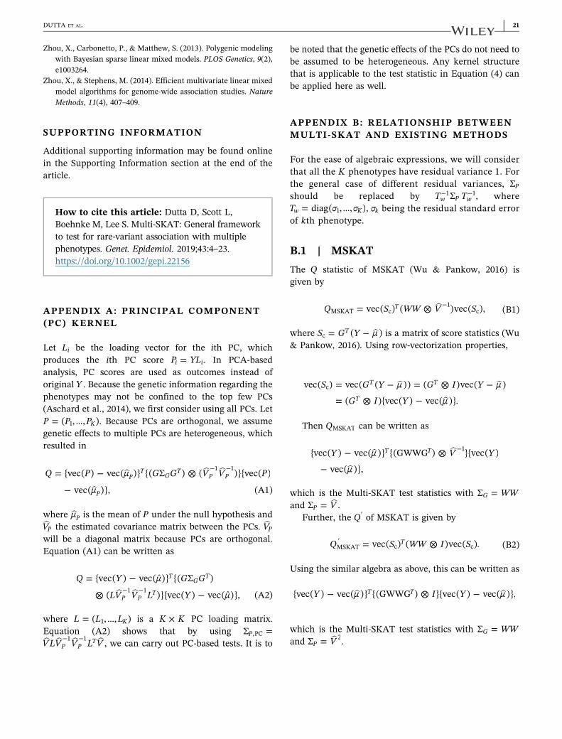
APPENDIX A: PRINCIPAL COMPONENT(PC) KERNEL

Let Li be the loading vector for the ith PC, whichproduces the ith PC score P YL=i i. In PCA‐basedanalysis, PC scores are used as outcomes instead oforiginal Y . Because the genetic information regarding thephenotypes may not be confined to the top few PCs(Aschard et al., 2014), we first consider using all PCs. LetP P P= ( , …, )K1 . Because PCs are orthogonal, we assumegenetic effects to multiple PCs are heterogeneous, whichresulted in

⊗Q P μ G G V V P

μ

= vec( ) − vec( ) ( Σ ) ( )vec( )

− vec( ),P

TG

TP P

P

−1 −1

(A1)

where μP is the mean of P under the null hypothesis andVP the estimated covariance matrix between the PCs. VPwill be a diagonal matrix because PCs are orthogonal.Equation (A1) can be written as

⊗

Q Y μ G G

LV V L Y μ

= vec( ) − vec( ˆ) ( Σ )

( )vec( ) − vec( ˆ),

TG

T

P PT−1 −1

(A2)

where L L L= ( , …, )K1 is a K K× PC loading matrix.Equation (A2) shows that by using Σ =P,PC V LV V L VP P

T−1 −1, we can carry out PC‐based tests. It is to

be noted that the genetic effects of the PCs do not need tobe assumed to be heterogeneous. Any kernel structurethat is applicable to the test statistic in Equation (4) canbe applied here as well.

APPENDIX B: RELATIONSHIP BETWEENMULTI ‐SKAT AND EXISTING METHODS

For the ease of algebraic expressions, we will considerthat all the K phenotypes have residual variance 1. Forthe general case of different residual variances, ΣPshould be replaced by T TΣw P w

−1 −1, whereT σ σ= diag( , …, )w K1 , σk being the residual standard errorof kth phenotype.

B.1 | MSKAT

The Q statistic of MSKAT (Wu & Pankow, 2016) isgiven by

⊗Q S WW V S= vec( ) ( )vec( ),TMSKAT c

−1c (B1)

where S G Y μ= ( − )Tc is a matrix of score statistics (Wu

& Pankow, 2016). Using row‐vectorization properties,

⊗

⊗

S G Y μ G I Y μ

G I Y μ

vec( ) = vec( ( − )) = ( )vec( − )

= ( )vec( ) − vec( ).

T T

T

c

Then QMSKAT can be written as

⊗Y μ V Y

μ

vec( ) − vec( ) (GWWG ) vec( )

− vec( ),

T T −1

which is the Multi‐SKAT test statistics with WWΣ =Gand VΣ =P .

Further, the Q′ of MSKAT is given by

⊗Q S WW I S= vec( ) ( )vec( ).TMSKAT′

c c (B2)

Using the similar algebra as above, this can be written as

⊗Y μ I Y μvec( ) − vec( ) (GWWG ) vec( ) − vec( ),T T

which is the Multi‐SKAT test statistics with WWΣ =Gand VΣ =P

2.

DUTTA ET AL. | 21

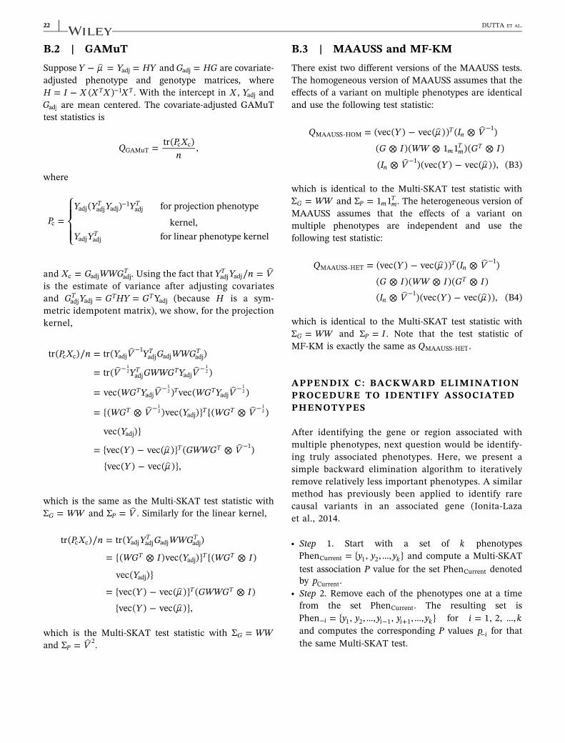
B.2 | GAMuT

Suppose Y μ Y HY− = =adj and G HG=adj are covariate‐adjusted phenotype and genotype matrices, whereH I X X X X= − ( )T T−1 . With the intercept in X , Yadj andGadj are mean centered. The covariate‐adjusted GAMuTtest statistics is

Q P Xn

= tr( ) ,GAMuTc c

where

⎧⎨⎪⎪

⎩⎪⎪

PY Y Y Y

Y Y

=( ) for projection phenotype

kernel,for linear phenotype kernel

T T

Tc

adj adj adj−1

adj

adj adj

and X G WWG= Tc adj adj. Using the fact that ∕Y Y n V=T

adj adjis the estimate of variance after adjusting covariatesand G Y G HY G= = YT T T

adj adj adj (because H is a sym-metric idempotent matrix), we show, for the projectionkernel,

∕

⊗ ⊗

⊗

P X n Y V Y G WWG

V Y GWWG Y V

WG Y V WG Y V

WG V Y WG V

Y

Y μ GWWG V

Y μ

tr( ) = tr( )

= tr( )

= vec( ) vec( )

= ( )vec( ) ( )

vec( )

= vec( ) − vec( ) ( )

vec( ) − vec( ),

T T

T T

T T T

T T T

T T

c c adj−1

adj adj adj

−adj adj

−

adj−

adj−

−adj

−

adj

−1

12

12

12

12

12

12

which is the same as the Multi‐SKAT test statistic withWWΣ =G and VΣ =P . Similarly for the linear kernel,

∕

⊗ ⊗

⊗

P X n Y Y G WWG

WG I Y WG I

Y

Y μ GWWG I

Y μ

tr( ) = tr( )

= ( )vec( ) ( )

vec( )

= vec( ) − vec( ) ( )

vec( ) − vec( ),

T T

T T T

T T

c c adj adj adj adj

adj

adj

which is the Multi‐SKAT test statistic with WWΣ =Gand VΣ =P

2.

B.3 | MAAUSS and MF‐KM

There exist two different versions of the MAAUSS tests.The homogeneous version of MAAUSS assumes that theeffects of a variant on multiple phenotypes are identicaland use the following test statistic:

⊗

⊗ ⊗ ⊗

⊗

Q Y μ I V

G I WW G I

I V Y μ

= (vec( ) − vec( )) ( )

( )( 1 1 )( )

( )(vec( ) − vec( )),

Tn

m mT T

n

MAAUSS‐HOM−1

−1 (B3)

which is identical to the Multi‐SKAT test statistic withWWΣ =G and Σ = 1 1P m m

T . The heterogeneous version ofMAAUSS assumes that the effects of a variant onmultiple phenotypes are independent and use thefollowing test statistic:

⊗

⊗ ⊗ ⊗

⊗

Q Y μ I V

G I WW I G I

I V Y μ

= (vec( ) − vec( )) ( )

( )( )( )

( )(vec( ) − vec( )),

Tn

T

n

MAAUSS‐HET−1

−1 (B4)

which is identical to the Multi‐SKAT test statistic withWWΣ =G and IΣ =P . Note that the test statistic of

MF‐KM is exactly the same as QMAAUSS‐HET.

APPENDIX C: BACKWARD ELIMINATIONPROCEDURE TO IDENTIFY ASSOCIATEDPHENOTYPES

After identifying the gene or region associated withmultiple phenotypes, next question would be identify-ing truly associated phenotypes. Here, we present asimple backward elimination algorithm to iterativelyremove relatively less important phenotypes. A similarmethod has previously been applied to identify rarecausal variants in an associated gene (Ionita‐Lazaet al., 2014.

• Step 1. Start with a set of k phenotypesy y yPhen = , , …, kCurrent 1 2 and compute a Multi‐SKAT

test association P value for the set PhenCurrent denotedby pCurrent.

• Step 2. Remove each of the phenotypes one at a timefrom the set PhenCurrent. The resulting set is

y y y y yPhen = , , …, , , …, i i i k− 1 2 −1 +1 for i k= 1, 2, …,and computes the corresponding P values p i− for thatthe same Multi‐SKAT test.

22 | DUTTA ET AL.

• Step 3. Remove the phenotype j that leads to thesmallest P value, that is, j p p p= argmin , , …, k−1 −2 − .

Update PhenCurrent to Phen j− .• Step 4. Continue removing phenotypes till only onephenotype is left.

Supporting Information Table S2 shows the back-ward elimination results of five most significant andsuggestive genes in the METSIM study data analysis asper the P values reported by minPcom. Although thisprocedure does not provide a set of phenotypes trulyassociated, it provides the relative importance of thephenotypes in driving association signals. For example,the minPcom P value for GLDC was 2.3 × 10−72. Wheneach of the phenotypes was removed one at a time andthe minPcom P values were calculated on the remainingeight phenotypes, we found that eliminating isoleucine

(Ile) actually improved the signal. The minPcom P valueof the set of eight amino acids leaving out Ile was2.8 × 10−73. This indicates that isoleucine has veryminimal contribution to the association between theamino acids and GLDC. Subsequently, valine was thenext phenotype to be eliminated indicating that it hasthe next lowest contribution after isoleucine. Carryingout this procedure further, we find that glycine is thelast phenotype to remain indicating that it is thestrongest driver of the signal. This is in agreement tothe single‐phenotype SKAT‐O results (Table 5). Simi-larly for genes HAL, DHODH, PAH, and MED1,histidine, alanine, phenylalanine, and tyrosine werethe most associated phenotypes, respectively. Interest-ingly for PAH and MED1, single‐phenotype P valuesare not significant, which suggests that multiplephenotypes are associated with these genes.

DUTTA ET AL. | 23