Multi-scale community organization of the human structural ...€¦ · Multi-scale communities in the human connectome 355 process, whereas the resolution parameters of Reichard &

Network Science 1 (3): 353–373, 2013. c© Cambridge University Press 2014. The online version of

this article is published within an Open Access environment subject to the conditions of the Creative

Commons Attribution licence http://creativecommons.org/licenses/by/3.0/

doi:10.1017/nws.2013.19

353

Multi-scale community organizationof the human structural connectome and

its relationship with resting-statefunctional connectivity

RICHARD F. BETZEL

Department of Psychological and Brain Sciences, Indiana University, Bloomington, IN, USA

Program in Cognitive Science, Indiana University, Bloomington, IN, USA

ALESSANDRA GRIFFA

Department of Radiology, University Hospital Center and University of Lausanne (CHUV),

Lausanne, Switzerland

Signal Processing Laboratory (LTS5), Ecole Polytechnique Federale de Lausanne (EPFL),


ANDREA AVENA-KOENIGSBERGER



JOAQU IN GON I


JEAN-PHIL IPPE THIRAN and PATRIC HAGMANN

Department of Radiology, University Hospital Center and University of Lausanne (CHUV),


Signal Processing Laboratory (LTS5), Ecole Polytechnique Federale de Lausanne (EPFL),


OLAF SPORNS



(e-mail: [email protected])

Abstract

The human connectome has been widely studied over the past decade. A principal finding

is that it can be decomposed into communities of densely interconnected brain regions. Past

studies have often used single-scale modularity measures in order to infer the connectome’s

community structure, possibly overlooking interesting structure at other organizational scales.

In this report, we used the partition stability framework, which defines communities in terms of

a Markov process (random walk), to infer the connectome’s multi-scale community structure.

Comparing the community structure to observed resting-state functional connectivity revealed

communities across a broad range of scales that were closely related to functional connectivity.

This result suggests a mapping between communities in structural networks, models of

influence-spreading and diffusion, and brain function. It further suggests that the spread of

influence among brain regions may not be limited to a single characteristic scale.

Keywords: connectome, community structure, multi-scale, Markov process, resting-state

at https://www.cambridge.org/core/terms. https://doi.org/10.1017/nws.2013.19Downloaded from https://www.cambridge.org/core. IP address: 54.39.106.173, on 12 Jun 2020 at 18:32:18, subject to the Cambridge Core terms of use, available

https://www.cambridge.org/core/terms

https://doi.org/10.1017/nws.2013.19

https://www.cambridge.org/core

354 R. F. Betzel et al.

1 Introduction

Many complex networks exhibit community structure, defined for example by

clustered edge distributions such that vertices (nodes) in the same community

preferentially link to one another (Guimera & Amaral, 2005; Girvan & Newman,

2002; Newman & Girvan, 2004). Examples of community structure can be found in

society as groups of friends, workplaces, cities, and states (Moody & White, 2003;

Freeman, 2004); in protein interaction networks as groups of co-functioning proteins

(Jonsson et al., 2006); and in the World Wide Web (WWW) as webpages sharing

many hyperlinks (Albert et al., 1999; Flake et al., 2002).

Detecting community structure is an important endeavor in network science.

Though there exist many methods for doing so, none has emerged as clearly

preeminent (for a review, see Fortunato, 2010). One of the most widely used methods

is to identify the vertex partition that maximizes the modularity quality function,

defined as the difference between observed and expected intra-community edge

density (Newman, 2006). Despite its widespread usage, modularity analysis suffers

from several drawbacks: maximization is NP-hard and identifying the optimal

partition is often practically impossible (Fortunato, 2010); solutions are sometimes

degenerate, with multiple partitions corresponding to the maximum modularity

(Good et al., 2010); and a resolution limit renders modularity “blind” to communities

below some characteristic scale (Fortunato & Barthelemy, 2007).

The first two problems are ubiquitous to most community detection algorithms and

are generally unavoidable. The resolution limit is more specific to quality functions

like modularity, but has been remedied in several instances by the inclusion of a

tunable resolution parameter, which controls the scale at which communities are

detected (Reichardt & Bornholdt, 2006; Arenas et al., 2008; Ronhovde & Nussinov,

2009) and has been generalized to include multi-slice networks (Mucha et al., 2010).

In neuroscience, multi-slice community detection has been studied in the context

of alterations in the community structure of functional brain networks over the

course of learning (Bassett et al., 2011). Outside of neuroscience, multi-scale/slice

community detection has been applied in fields including economics (Fenn et al.,

2009, 2012), protein interaction networks (Lewis et al., 2010; Delmotte et al., 2011),

and other examples of social and biological networks (Mucha et al., 2010; Onnela

et al., 2012).

This manuscript focuses on a particular multi-scale community detection algo-

rithm known as the partition stability framework, which defines communities in

terms of a Markov process based on a random walk model (Lambiotte et al.,

2008; Delvenne et al., 2010; Lambiotte, 2010). As this process evolves, a random

walker makes progressively longer walks and explores more distant parts of the

network. Intuitively, communities can be thought of as groups of vertices that

effectively “trap” the flow of random walkers over a particular timescale of the

random walk. In this way, the stability framework has been dubbed a “zooming

lens,” whereby focusing in on shorter or longer timescales reveals communities

of correspondingly smaller or larger diameter (Schaub et al., 2012). This method

can be mapped to the methods proposed by Reichardt & Bornholdt (2006) and

Arenas et al. (2008), indicating a mathematical equivalence. The partition stability

framework, however, differs conceptually from the other methods in a subtle way—

its resolution parameter (time) can be interpreted in the context of a random walk





Multi-scale communities in the human connectome 355

process, whereas the resolution parameters of Reichard & Bornholdt (2006) and

Arenas et al. (2008) were introduced ad hoc and have no additional interpretation.

The human connectome, i.e. the full set of neural elements and connections of the

human brain, can be modeled as a complex network (Sporns et al., 2005; Bullmore

& Sporns, 2009). The topological properties of this network have been studied for

nearly a decade, revealing key features including small-world architecture (Gong

et al., 2009), hub regions and cores (Hagmann et al., 2008), rich club organization

(van den Heuvel & Sporns, 2011), modular architecture (Chen et al., 2008; Meunier

et al., 2010; Wu et al., 2011), and economical wiring (Bassett et al., 2010; Bullmore

& Sporns, 2012). While these results characterize and contextualize the connectome

among all complex networks, the role of these topological features in shaping

communication processes and dynamic couplings among brain regions remains an

area of active research (Honey et al., 2009; van den Heuvel et al., 2012; Haimovici

et al., 2013).

Empirical and computational studies suggest that the human connectome under-

pins complex neural dynamics and facilitates the communication and integration

of information between brain regions. In functional magnetic resonance imaging

(fMRI), such “functional connectivity” is reflected by the magnitude of statistical

dependence, commonly measured as linear correlation, between blood oxygen-level

dependent (BOLD) signals recorded from different brain regions. A growing body

of literature describes patterns of resting-state functional connectivity (rsFC), i.e.

spontaneous, endogenous fluctuations of the BOLD signal in the absence of any

explicit cognitive task. This work has revealed consistent connectivity patterns,

dubbed resting-state networks (RSN), which resemble networks of regions (e.g.,

somato-motor, visual, default mode, etc.) that are coherently engaged in various

cognitive and behavioral domains (Greicius et al., 2003; Damoiseaux et al., 2006;

Fox & Raichle, 2007; Smith et al., 2009).

This article has two principal aims. The first aim consists of detecting and

characterizing the multi-scale community structure of the human connectome using

the partition stability framework. The second aim is to assess the relationship of

such structure to empirically observed rsFC. Where the first aim attempts to answer

the question “what communities of brain regions are situated in such a way that

they could take advantage of a diffusion-like process in order to pass information or

spread influence among themselves,” the second aim attempts to answer the question

“what evidence is there that the previously-identified communities match observed

patterns of functional connectivity and at which scales is the correspondence between

community structure and functional coupling most salient?”

2 Methods

2.1 Neuroimaging and data acquisition

Forty (40) healthy human volunteers (24 males and 16 females, 25.3 ± 4.9 years old)

underwent an MRI session on a 3-Tesla scanner (Trio, Siemens Medical, Germany)

with a 32-channel head-coil. The session consisted of (i) a magnetization-prepared

rapid acquisition gradient echo (MPRAGE) sequence sensitive to white/gray matter

contrast (1 mm in-plane resolution, 1.2 mm slice thickness), (ii) a diffusion spectrum

imaging (DSI) sequence (128 diffusion weighted volumes +1 reference b0 volume,






maximum b-value 8000 s/mm2, 2.2 × 2.2 × 3.0 mm voxel size), and (iii) a gradient

echo EPI sequence sensitive to BOLD contrast (3.3 mm in-plane resolution and slice

thickness with a 0.3 mm gap, TR 1920 ms). During the fMRI acquisition, subjects

were lying in the scanner with eyes open, resting but awake and cognitively alert,

thus recording-resting-state fMRI (rs-fMRI). The acquisition process resulted in a

sequence of 276 BOLD images for each subject.

DSI, rs-fMRI, and MPRAGE data were processed using the Connectome Map-

ping Toolkit (Daducci et al., 2012). Each participant’s gray and white matter

compartments were segmented from the MPRAGE volume. The entire cortical and

subcortical volume was subdivided into 1015 equal sized regions of interest (Cam-

moun et al., 2012). The present study, however, focused on cortical structures only,

and discarded subcortical regions including the bilateral thalamus, caudate, putamen,

pallidum, accumbens, hippocampus, and amygdala, as well as the brainstem, result-

ing in 1000 cortical regions of interest. Each region, in turn, could be mapped to one

of 68 cortical areas, with 34 areas per hemisphere (for a complete list of cortical areas

and their mapping to regions of interest, see the Supplementary Information). Whole

brain streamline tractography was performed on reconstructed DSI data (Wedeen

et al., 2008), and participant-wise, right hemisphere connectivity matrices were

estimated by selecting the streamlines connecting each pair of 501 cortical regions

in the right hemisphere. Connectivity strength between each pair of regions was

quantified as fiber density, which is defined as the number of streamlines connecting

the two regions, normalized by the average streamline’s length, and the average

surface of the two connected areas (Hagmann et al., 2008). The normalization by the

average streamline’s length is meant to compensate for the bias toward longer fibers

introduced by the tractography algorithm. The connectivity values quantified as fiber

density were used to construct subject-wise structural connectivity (SC) matrices.

Each SC matrix can be interpreted as the adjacency matrix Aij of a graph

G ≡ {V , E}, with vertices V = {v1, . . . , vn} corresponding to cortical regions of

interest, and weighted, undirected edges E = {eij , . . . , ekl} representing anatomical

connections. This network is often referred to as a structural connectome. It is

convenient at this point to define a connectome’s vertex strength and total weight

as si = ΣjAij and m = 12ΣijAij , respectively.

Functional data were pre-processed according to state of the art pipelines (Murphy

et al., 2009; Power et al., 2012). The raw fMRI volumes were motion-corrected

by applying rigid body co-registration. Voxel-wise signals were then corrected for

physiological confounds and artifacts by regressing out the average white matter

signal, the average cerebrospinal fluid signal, and the six motion signals (three

translations and three rotations) previously estimated. The time series were low-

pass filtered (temporal Gaussian filter with full width at half maximum = 1.92 s),

and the first four time points were excluded to allow signal stabilization. No

spatial smoothing was applied. Following “motion scrubbing” (Power et al., 2012),

voxel-wise fMRI signals were averaged across each cortical region in order to

obtain a representative time series for each region. The functional connectivity

between each pair of regions was estimated as the Pearson correlation between

the corresponding average signals. A single, right hemisphere rsFC matrix Fij

representative of the whole group of participants was computed by averaging the 40

individual correlation matrices. The group-mean structural connectome (weighted

and binary) and functional connectivity matrix for the right hemisphere of cerebral






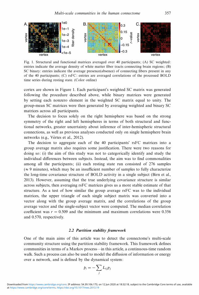
Fig. 1. Structural and functional matrices averaged over 40 participants; (A) SC weighted:

entries indicate the average density of white matter fiber tracts connecting brain regions; (B)

SC binary: entries indicate the average presence(absence) of connecting fibers present in any

of the 40 participants; (C) rsFC: entries are averaged correlations of the processed BOLD

time series during resting state. (Color online)

cortex are shown in Figure 1. Each participant’s weighted SC matrix was generated

following the procedure described above, while binary matrices were generated

by setting each nonzero element in the weighted SC matrix equal to unity. The

group-mean SC matrices were then generated by averaging weighted and binary SC

matrices across all participants.

The decision to focus solely on the right hemisphere was based on the strong

symmetry of the right and left hemispheres in terms of both structural and func-

tional networks, greater uncertainty about inference of inter-hemispheric structural

connections, as well as previous analyses conducted only on single hemisphere brain

networks (e.g., Vertes et al., 2012).

The decision to aggregate each of the 40 participants’ rsFC matrices into a

group average matrix also requires some justification. There were two reasons for

doing so: (i) the aim of this study was not to categorically identify and study the

individual differences between subjects. Instead, the aim was to find commonalities

among all the participants; (ii) each resting state run consisted of 276 samples

(≈ 9 minutes), which may be an insufficient number of samples to fully characterize

the long-time covariance structure of BOLD activity in a single subject (Birn et al.,

2013). However, assuming that the true underlying covariance structure is similar

across subjects, then averaging rsFC matrices gives us a more stable estimate of that

structure. As a test of how similar the group average rsFC was to the individual

matrices, the upper triangle of each single subject matrix was converted into a

vector along with the group average matrix, and the correlations of the group

average vector and the single-subject vector were computed. The median correlation

coefficient was r = 0.509 and the minimum and maximum correlations were 0.356

and 0.570, respectively.

2.2 Partition stability framework

One of the main aims of this article was to detect the connectome’s multi-scale

community structure using the partition stability framework. This framework defines

communities in terms of a Markov process—in this article, a continuous-time random

walk. Such a process can also be used to model the diffusion of information or energy

over a network, and is defined by the dynamical system:

pi = − ∑j

Lijpj






where pi is the probability of finding a random walker on vertex vi and Lij =

δij − Aij/sj is the normalized graph Laplacian matrix. If the network is undirected

and connected, this system evolves to the equilibrium state p∗i = si/2m.

The stability framework detects community structure at different timescales of

the random walk (referred to simply as “scales” so as to avoid any confusion with

time in the context of intrinsic brain dynamics). The communities were detected by

identifying the vertex partition that maximizes the quality function “stability.” Let

℘ = {C1, . . . ,CK} be a partition of V into K communities, such that Ci ∩Cj = ∅ and

∪i Ci = V . The stability of ℘ at a given scale t is defined as:

R (℘, t) =∑C∈℘

∑ij∈C

[(e−tL)ijp

∗j − p∗

i p∗j

]

where the summation extends over all communities and the edges that fall within

each community. The first term in the summation, (e−tL)ijp∗j , is the probability that

a random walker starting in community C will be in that community at scale t. The

second term p∗i p

∗j is the probability that two independent random walkers will be

in C at equilibrium. The difference in these terms represents the density of random

walkers in a community in excess of what is expected at equilibrium. Key to this

framework, the stability measurement depends not only on the partition ℘, but also

on the scale t. In general, different partitions will maximize stability at different

scales in the random walk. Varying t across scales and maximizing stability recovers

the community structure at each scale.

The process of optimizing R(℘, t) can be accomplished in a number of ways. One

appealing option, and the one used in this article, makes use of the relationship

between partition stability and a more widely used modularity measure. Lambiotte

et al. (2008, 2011) demonstrated that stability could be recast in terms of the

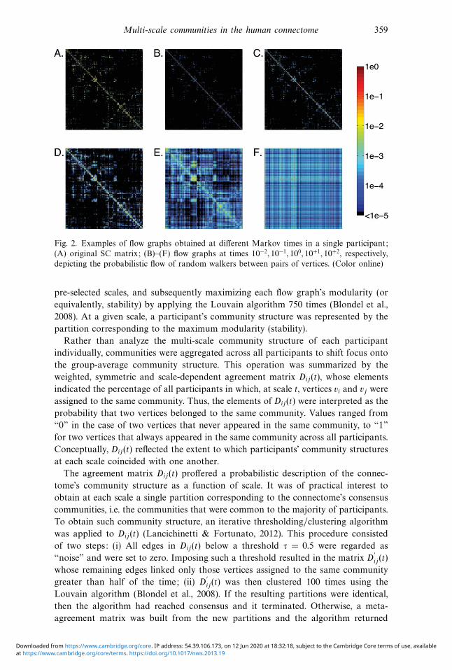
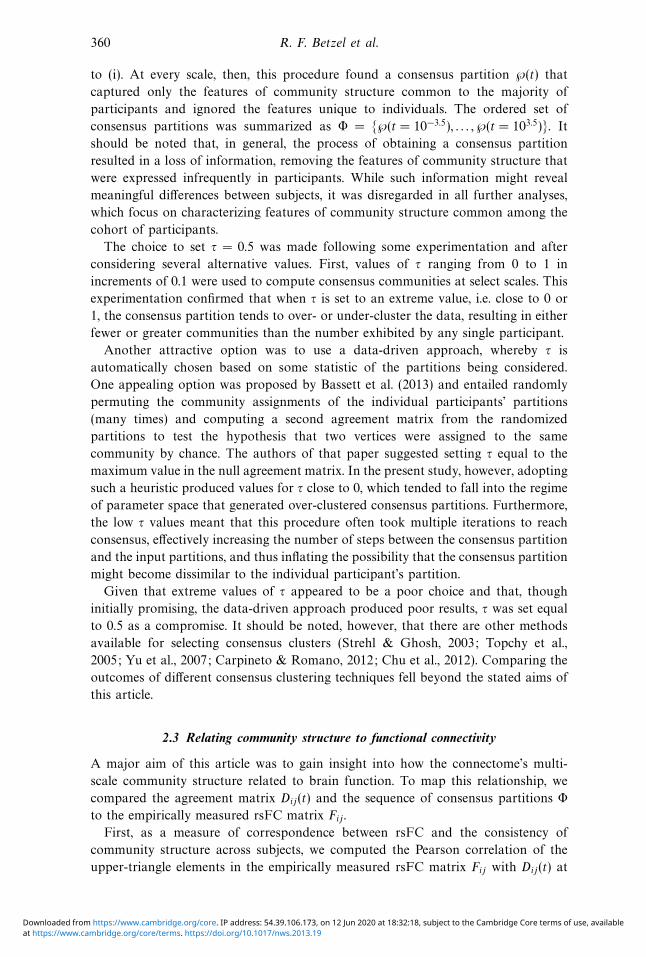
modularity of a weighted, symmetric “flow graph.” A flow graph is a transformation

of Aij in which the dynamics of a Markov process are embedded into the edges

of a new graph. In the case of a continuous-time random walk, the flow graph is

represented by the full matrix A′ij(t) = (e−tL)ijsj whose elements are proportional

to the probabilistic flow of random walkers between vertices at scale t. Examples

of flow graphs for one of the participants are shown in Figure 2. The relationship

between stability and modularity is such that instead of directly maximizing R(℘, t),

one can equivalently maximize the modularity of a flow graph evaluated at scale t:

Q (℘, t) =1

2m

∑C∈℘

∑ij∈C

[A′ij (t) − sisj

2m

]

This result confers the practical advantage that any heuristic previously used to

maximize modularity can now be repurposed in order to maximize stability.

To apply this set of principles to the connectomes obtained from 40 healthy indi-

viduals, a range of scales had to be selected over which to maximize stability. After

experimentation, it was determined that at scales below t = 10−3.5, every participant’s

community structure was characterized by a partition into n communities, i.e. every

vertex was assigned to its own community, and at scales greater than t = 103.5 every

participant exhibited a two-community division. Using these scales as lower and

upper boundaries, we selected 185 logarithmically spaced points over the interval

[10−3.5, 103.5] at which to maximize partition stability. This process entailed defining

a flow graph A′ij(t) for each participant, evaluating that flow graph at each of the






Fig. 2. Examples of flow graphs obtained at different Markov times in a single participant;

(A) original SC matrix; (B)–(F) flow graphs at times 10−2, 10−1, 100, 10+1, 10+2, respectively,

depicting the probabilistic flow of random walkers between pairs of vertices. (Color online)

pre-selected scales, and subsequently maximizing each flow graph’s modularity (or

equivalently, stability) by applying the Louvain algorithm 750 times (Blondel et al.,

2008). At a given scale, a participant’s community structure was represented by the

partition corresponding to the maximum modularity (stability).

Rather than analyze the multi-scale community structure of each participant

individually, communities were aggregated across all participants to shift focus onto

the group-average community structure. This operation was summarized by the

weighted, symmetric and scale-dependent agreement matrix Dij(t), whose elements

indicated the percentage of all participants in which, at scale t, vertices vi and vj were

assigned to the same community. Thus, the elements of Dij(t) were interpreted as the

probability that two vertices belonged to the same community. Values ranged from

“0” in the case of two vertices that never appeared in the same community, to “1”

for two vertices that always appeared in the same community across all participants.

Conceptually, Dij(t) reflected the extent to which participants’ community structures

at each scale coincided with one another.

The agreement matrix Dij(t) proffered a probabilistic description of the connec-

tome’s community structure as a function of scale. It was of practical interest to

obtain at each scale a single partition corresponding to the connectome’s consensus

communities, i.e. the communities that were common to the majority of participants.

To obtain such community structure, an iterative thresholding/clustering algorithm

was applied to Dij(t) (Lancichinetti & Fortunato, 2012). This procedure consisted

of two steps: (i) All edges in Dij(t) below a threshold τ = 0.5 were regarded as

“noise” and were set to zero. Imposing such a threshold resulted in the matrix D′ij(t)

whose remaining edges linked only those vertices assigned to the same community

greater than half of the time; (ii) D′ij(t) was then clustered 100 times using the

Louvain algorithm (Blondel et al., 2008). If the resulting partitions were identical,

then the algorithm had reached consensus and it terminated. Otherwise, a meta-

agreement matrix was built from the new partitions and the algorithm returned






to (i). At every scale, then, this procedure found a consensus partition ℘(t) that

captured only the features of community structure common to the majority of

participants and ignored the features unique to individuals. The ordered set of

consensus partitions was summarized as Φ = {℘(t = 10−3.5), . . . , ℘(t = 103.5)}. It

should be noted that, in general, the process of obtaining a consensus partition

resulted in a loss of information, removing the features of community structure that

were expressed infrequently in participants. While such information might reveal

meaningful differences between subjects, it was disregarded in all further analyses,

which focus on characterizing features of community structure common among the

cohort of participants.

The choice to set τ = 0.5 was made following some experimentation and after

considering several alternative values. First, values of τ ranging from 0 to 1 in

increments of 0.1 were used to compute consensus communities at select scales. This

experimentation confirmed that when τ is set to an extreme value, i.e. close to 0 or

1, the consensus partition tends to over- or under-cluster the data, resulting in either

fewer or greater communities than the number exhibited by any single participant.

Another attractive option was to use a data-driven approach, whereby τ is

automatically chosen based on some statistic of the partitions being considered.

One appealing option was proposed by Bassett et al. (2013) and entailed randomly

permuting the community assignments of the individual participants’ partitions

(many times) and computing a second agreement matrix from the randomized

partitions to test the hypothesis that two vertices were assigned to the same

community by chance. The authors of that paper suggested setting τ equal to the

maximum value in the null agreement matrix. In the present study, however, adopting

such a heuristic produced values for τ close to 0, which tended to fall into the regime

of parameter space that generated over-clustered consensus partitions. Furthermore,

the low τ values meant that this procedure often took multiple iterations to reach

consensus, effectively increasing the number of steps between the consensus partition

and the input partitions, and thus inflating the possibility that the consensus partition

might become dissimilar to the individual participant’s partition.

Given that extreme values of τ appeared to be a poor choice and that, though

initially promising, the data-driven approach produced poor results, τ was set equal

to 0.5 as a compromise. It should be noted, however, that there are other methods

available for selecting consensus clusters (Strehl & Ghosh, 2003; Topchy et al.,

2005; Yu et al., 2007; Carpineto & Romano, 2012; Chu et al., 2012). Comparing the

outcomes of different consensus clustering techniques fell beyond the stated aims of

this article.

2.3 Relating community structure to functional connectivity

A major aim of this article was to gain insight into how the connectome’s multi-

scale community structure related to brain function. To map this relationship, we

compared the agreement matrix Dij(t) and the sequence of consensus partitions Φ

to the empirically measured rsFC matrix Fij .

First, as a measure of correspondence between rsFC and the consistency of

community structure across subjects, we computed the Pearson correlation of the

upper-triangle elements in the empirically measured rsFC matrix Fij with Dij(t) at






each scale t. Larger correlation values implied that the propensity for two vertices to

share a community assignment was a good predictor of whether those same vertices

were also functionally coupled. It should be noted that this measurement does not

establish a direct link between community structure and rsFC, but instead links the

reliability of community structure to rsFC.

As a second measure of correspondence, each consensus community’s “goodness”

was determined by imposing it upon the rsFC matrix Fij . Conceptually, a “good”

community was one whose internal density of positive functional connections and

external negative connections were greater than expected by chance. This intuition

of a community’s “goodness” was in line with definitions of modularity adopted for

use with signed networks (Traag & Bruggeman, 2009; Rubinov & Sporns, 2011).

Therefore, a consensus community’s “goodness” with respect to rsFC was estimated

by computing its modularity score. The modularity of a community in a signed

network is defined as:

q∗C =1

2m+

∑ij∈C

[F+ij − sisj

2m+

]− 1

2m+ + 2m−∑ij∈C

[F−ij − s−

i s−j

2m−

]

where F±ij are rsFC matrices comprised of only positive (+) and negative (–)

connections, s±i =

∑j F

±ij is the signed vertex strengths, and m± = 1

2

∑ij F

±ij is the

total signed weight of the network.

Large communities, because they consisted of many vertices, also tended to have

large modularity scores. To remove this bias, the procedure described above was

repeated 5,000 times but with vertices randomly assigned to communities Crand,

each time resulting in a measurement q∗Crand. This score enabled estimates of the

expected value (E[q∗Crand]) and variance (σ[q∗Crand

]) of each community’s modularity

score to be obtained. From these estimates, a community’s score was standardized

and expressed as a z-score:

z∗C =(q∗C − E[q∗Crand

])

σ[q∗Crand]

The score zC was interpreted as an indicator of how well each structural community

C ∈ ℘(t) mapped onto rsFC. A large, positive zC indicated that a community’s

signed modularity was much greater than would be expected given its size.

In addition to identifying communities that were more modular than by chance,

the scores zC were useful for answering several important questions about how

stability-derived communities related to rsFC: (i) On average which cortical areas

contributed the most standardized modularity; (ii) which pairs of vertices; and (iii)

which pairs of cortical areas, when assigned to the same community, portended a

large standardized modularity score for that community.

From the set of standardized modularity scores, it was straightforward to compute

the total standardized modularity contribution of each cortical area by summing

the scores of each vertex vi over all communities in which vi participated and then

aggregating these scores by cortical area.

Another important question was how the co-assignment of groups of vertices or

cortical areas to a given community influenced that community’s modularity. For

example, does assigning vertices vi and vj to the same community portend a higher

or lower modularity for that community? To identify such groups, a matrix Tij






was built and subsequently clustered. Initially, the weights of Tij were set to zero.

The weights were updated by considering each community C and strengthening the

connections among all of the vertices assigned to C by zC. For example, suppose a

community C was comprised of vertices 1–10 and that this community’s previously

measured standardized modularity score was zC = 3. Were this the case, then the

elements Tij for i, j = 1, . . . , 10 would be uniformly increased by zC = 3. This process

would be repeated for each community in the set of all communities, Φ. Thus, the

weights of Tij were equal to the sum of standardized modularity over all communities

in which vertices vi and vj both appeared. An agglomerative, hierarchical clustering

algorithm was then used to extract groups of vertices that collectively influenced

a community’s modularity (Hastie et al., 2001). This algorithm treated each row

in Tij as a feature vector of the matching vertex vi. Starting with every vertex

in its own cluster, clusters were merged over a series of steps until only two

clusters remained. At each step, the relationship between every pair of clusters was

defined by the average Euclidean distance between the feature vectors of vertices

assigned to those clusters. The heuristic for merging clusters was to identify the

two clusters whose distance was smallest and to combine their elements, forming

a larger joint cluster at the next step. This procedure produced a hierarchical tree

of related vertices which can be thresholded, revealing a finer or coarser clustering

depending on the level of the threshold. At any level, however, these clusters were

interpreted as groups of vertices that collectively participated in communities with

large standardized modularity scores. To identify pairs of cortical areas whose co-

assignment contributed to a community’s having small or large modularity, Tij was

down-sampled by aggregating its rows and columns according to cortical areas.

3 Results

The previous section described a procedure for identifying the connectome’s multi-

scale community structure using the partition stability framework. The association

between this structure and observed functional connectivity was assessed by corre-

lating it with rsFC and, separately, by measuring how well consensus communities

modularized the rsFC matrix.

Maximizing partition stability at 185 different scales logarithmically spaced over

the range [10−3.5, 10+3.5] generated a sequence of partitions for each participant.

Each sequence began at the shortest dynamical scale with the partition in which

every vertex comprised its own community. A division of the vertex set into two

communities characterized the final partition in each sequence, corresponding to the

largest scale. From these partition sequences, a number of statistics were computed

at each scale, specifically, the mean and standard deviation of the partition stability,

number of communities, community size, and number of singleton communities.

Partition stability and the number of communities declined monotonically while

the size of communities increased. The number of singleton communities declined

initially, before the maximum number of non-singleton communities reached a

maximum value at the scale t = 10−1.845 (Figure 3).

An iterative thresholding/reclustering algorithm was used to generate from

the participants’ partitions a sequence of consensus partitions, which represented

the “backbone” community structure. Typically, this procedure required only one






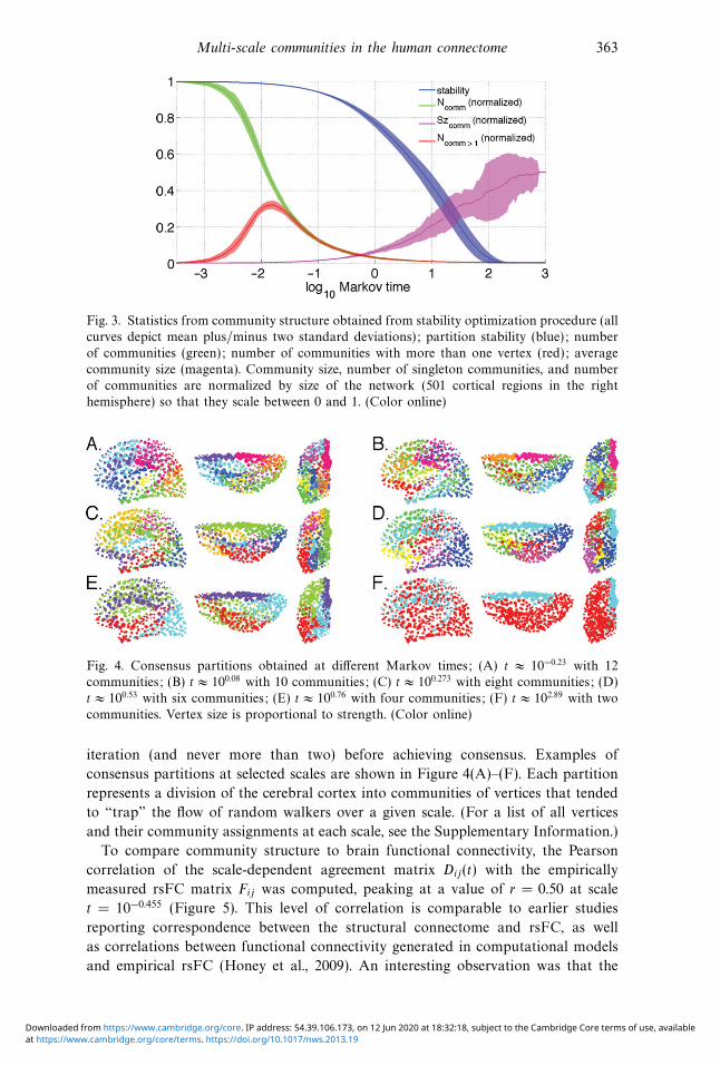
Fig. 3. Statistics from community structure obtained from stability optimization procedure (all

curves depict mean plus/minus two standard deviations); partition stability (blue); number

of communities (green); number of communities with more than one vertex (red); average

community size (magenta). Community size, number of singleton communities, and number

of communities are normalized by size of the network (501 cortical regions in the right

hemisphere) so that they scale between 0 and 1. (Color online)

Fig. 4. Consensus partitions obtained at different Markov times; (A) t ≈ 10−0.23 with 12

communities; (B) t ≈ 100.08 with 10 communities; (C) t ≈ 100.273 with eight communities; (D)

t ≈ 100.53 with six communities; (E) t ≈ 100.76 with four communities; (F) t ≈ 102.89 with two

communities. Vertex size is proportional to strength. (Color online)

iteration (and never more than two) before achieving consensus. Examples of

consensus partitions at selected scales are shown in Figure 4(A)–(F). Each partition

represents a division of the cerebral cortex into communities of vertices that tended

to “trap” the flow of random walkers over a given scale. (For a list of all vertices

and their community assignments at each scale, see the Supplementary Information.)

To compare community structure to brain functional connectivity, the Pearson

correlation of the scale-dependent agreement matrix Dij(t) with the empirically

measured rsFC matrix Fij was computed, peaking at a value of r = 0.50 at scale

t = 10−0.455 (Figure 5). This level of correlation is comparable to earlier studies

reporting correspondence between the structural connectome and rsFC, as well

as correlations between functional connectivity generated in computational models

and empirical rsFC (Honey et al., 2009). An interesting observation was that the






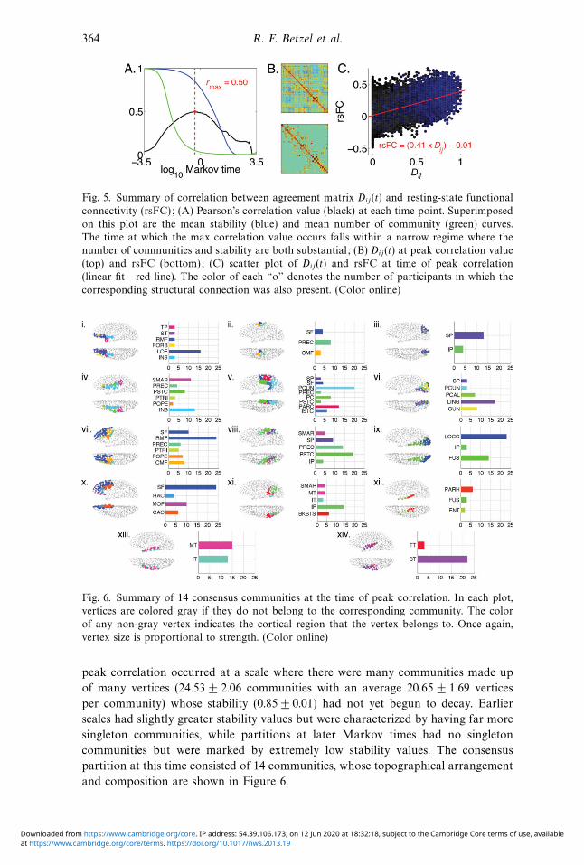
Fig. 5. Summary of correlation between agreement matrix Dij(t) and resting-state functional

connectivity (rsFC); (A) Pearson’s correlation value (black) at each time point. Superimposed

on this plot are the mean stability (blue) and mean number of community (green) curves.

The time at which the max correlation value occurs falls within a narrow regime where the

number of communities and stability are both substantial; (B) Dij(t) at peak correlation value

(top) and rsFC (bottom); (C) scatter plot of Dij(t) and rsFC at time of peak correlation

(linear fit—red line). The color of each “o” denotes the number of participants in which the

corresponding structural connection was also present. (Color online)

Fig. 6. Summary of 14 consensus communities at the time of peak correlation. In each plot,

vertices are colored gray if they do not belong to the corresponding community. The color

of any non-gray vertex indicates the cortical region that the vertex belongs to. Once again,

vertex size is proportional to strength. (Color online)

peak correlation occurred at a scale where there were many communities made up

of many vertices (24.53 ± 2.06 communities with an average 20.65 ± 1.69 vertices

per community) whose stability (0.85 ± 0.01) had not yet begun to decay. Earlier

scales had slightly greater stability values but were characterized by having far more

singleton communities, while partitions at later Markov times had no singleton

communities but were marked by extremely low stability values. The consensus

partition at this time consisted of 14 communities, whose topographical arrangement

and composition are shown in Figure 6.






Fig. 7. Summary of modularity scores of communities at different times; (A) sum of

positive and negative normalized scores by vertex over time; (B) weighted matrix where

each community co-assignment was weighted by its score; (C) anatomical area average and

peak standardized modularity score; (D) weighted agreement matrix aggregated across by

anatomical area. (Color online)

As a second means of relating community structure to observed functional

connectivity, we measured the extent to which consensus communities were also

good functional communities. This process consisted of estimating every consensus

community’s standardized modularity score. Over a range of scales from t ≈ 10−1.5

to t ≈ 102.5, a number of communities had much greater-than-expected modularity

(Figure 7(A)). Mapping these scores onto brain anatomy and summing across scales,

it was observed that every cortical area contributed positive modularity, though

some contributed disproportionately more (Figure 7(C)). The areas contributing the

greatest modularity (both in terms of peak value and total contribution) were found

to be the precentral and postcentral cortex, the lateral occipital cortex, the superior

parietal cortex, and lingual cortex. Other areas also had large values, including the

rostral middle-frontal cortex, superior frontal cortex, the inferior parietal cortex, as

well as the superior temporal, supramarginal, and fusiform cortex.

The matrix Tij was constructed to measure the pairs of vertices that collectively

participated in communities with greater-than-expected modularity (Figure 7(B)).






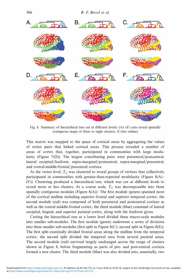
Fig. 8. Summary of hierarchical tree cut at different levels; (A)–(F) cuts reveal spatially

contiguous maps of three to eight clusters. (Color online)

This matrix was mapped to the space of cortical areas by aggregating the values

of vertex pairs that linked cortical areas. This process revealed a number of

areas of cortex that, together, participated in communities with large modu-

larity (Figure 7(D)). The largest contributing pairs were precentral/postcentral,

lateral occipital/fusiform, supra-marginal/postcentral, supra-marginal/precentral,

and rostral-middle-frontal/precentral cortices.

At the vertex level, Tij was clustered to reveal groups of vertices that collectively

participated in communities with greater-than-expected modularity (Figure 8(A)–

(F)). Clustering produced a hierarchical tree, which was cut at different levels to

reveal more or less clusters. At a coarse scale, Tij was decomposable into three

spatially contiguous modules (Figure 8(A)): The first module (green) spanned most

of the cortical midline including superior frontal and superior temporal cortex; the

second module (red) was composed of both precentral and postcentral cortices as

well as the rostral middle-frontal cortex; the third module (blue) consisted of lateral

occipital, lingual, and superior parietal cortex, along with the fusiform gyrus.

Cutting the hierarchical tree at a lower level divided these macro-scale modules

into smaller sub-modules. The first module (green) underwent a series of divisions

into three smaller sub-modules (first split in Figure 8(C); second split in Figure 8(E)).

The first split essentially divided frontal areas along the midline from the temporal

cortex; the second split divided the temporal area from several parietal areas.

The second module (red) survived largely unchanged across the range of clusters

shown in Figure 8, before fragmenting as parts of pre- and post-central cortices

formed a new cluster. The third module (blue) was also divided into, essentially, two






sub-modules, the first made up predominantly by the lingual cortex, and the second

made up of the fusiform area, lateral occipital, and superior parietal cortices. In

principle, Tij could be decomposed further until the number of modules was equal

to the number of vertices in the network.

4 Discussion

In this paper, we used the partition stability framework to infer multi-scale com-

munity structure in the human cerebral cortex. This procedure generated a series

of communities over a range of scales, beginning with a large number of small

communities (fine-scale) and ending with a small number of large communities

(coarse-scale). We compared communities derived from structural connectivity to

brain functional networks using two approaches: (i) We identified a scale at which the

Pearson correlation of an agreement matrix with empirically measured rsFC became

maximal, with a peak correlation of approximately r = 0.50; (ii) We evaluated

the modularity of each consensus community when it was imposed on rsFC, and

identified a number of communities that overlapped with rsFC modules. These

results suggest that a community’s position in space and the scales over which

it appears, provide complementary information for assessing its importance and

relevance to network function.

Before discussing these results, it is worth explicitly stating our views of stability

maximization and its relationship to the human connectome and communication

processes in the brain. Communities derived from maximizing partition stability can

be interpreted in multiple ways. The first interpretation is based on the view that

stability maximization is simply a useful methodology for identifying community

structure across multiple scales; no special functional significance is attributed to

communities detected this way. The second interpretation regards such communities

as being important to a dynamical process (e.g., diffusion), i.e. communities reflect

the structural properties of a network that bias the trajectory of a random walker

exploring the network. If the random walk is, in some way, a suitable model of

the network’s intrinsic dynamics, then stability-derived communities take on even

more significance. In such a case, communities represent groups of nodes that more

readily communicate or exert influence over one another than they do with the rest

of the network. This paper adopts a view more closely aligned with the second

interpretation. The argument for doing so stems from a conceptualization of the

connectome as a communication network: Brain regions at different scales exert

certain influence over one another, and this influence is subserved by the anatomical

connections linking brain regions. This discussion asserts that it is, in part, the

connection topology that prescribes a region’s preference to functionally link to

another region, or for a group of regions to become mutually coupled. Hence, from

this point of view, identifying communities of vertices that are likely to influence

or communicate with one another is of great practical interest and can possibly

illuminate true functional dependencies. Nonetheless, it should be noted that the

relationship between intrinsic brain dynamics and diffusion/random-walk processes

remains in need of empirical testing.

The first major finding was that the correlation of the scale-dependent agreement

matrix, which reflected the consistency of community ties between vertices at a






given time point across all subjects, with rsFC reached a clear peak value. This

result owes its significance to the interpretation of community structure as a marker

of the propensity for vertices belonging to the same community to spread influence,

information, or energy among one another and not with the rest of the network.

Given this point of view, one can think of the peak correlation as corresponding to

the scale at which empirical functional couplings became most closely aligned with

influential communities that are consistently identified across subjects. This result is

significant, as the functional coupling of different brain regions has been interpreted

as integration of information (van den Heuvel & Hulshoff Pol, 2010).

The scale at which the peak correlation occurred is also particularly relevant as

it coincided with a regime characterized by partitions associated with large stability

values but also many non-singleton communities. At much earlier scales, the average

partition stability was slightly greater, but the number of singleton communities

vastly outnumbered the non-singleton communities. At later scales, stability tended

toward zero, so that even though the communities at those scales were much fewer

in number and contained more vertices, they were also more ill-defined than those at

earlier scales. This suggests that the peak correlation occurs within a fairly narrow

regime in which the number and size of communities strikes a balance with stability,

giving rise to a diverse, well-defined repertoire of communities.

The first result, however, only reveals part of the story. Linear correlation is

a measure of how closely two variables correspond to one another on average.

When examining the relationship between community structure and rsFC at the

level of individual communities, a different (but complementary) picture emerges.

Specifically, it was found that substantial variability existed in the timing of and

extent to which individual communities contributed to the modularization of the

rsFC matrix. Certain communities, even at scales where the partition as a whole

was only weakly related to rsFC, had exceptionally large standardized modularity.

At the time of the peak correlation, a large number of communities collectively

had substantial modularity, which likely contributed to the peak in the correlation

coefficient. This result, however, suggests that the relationship between rsFC and

community structure is not restricted to a single scale.

A third interesting finding concerns the relationship of community structure to

empirically observed resting state networks (RSN). The communities inferred here

were generally spatially contiguous due to the fact that the majority of structural

connections identified so far in the human connectome are short-distance and

connect nearby regions to one another. Therefore, it was unsurprising that distributed

and spatially non-contiguous RSNs, e.g., the right parietal-frontal and default mode

network, were never observed. However, highly modular communities were found

in occipital cortex, corresponding quite closely to the primary and extra-striate

visual RSNs (lingual gyrus, cuneus, lateral occipital, fusiform). Also observed were

high-modularity communities involving areas that are typically associated with the

somatomotor network (pre- and postcentral cortex). Interestingly, both visual and

somatomotor RSNs are generally classified as unimodal networks and thought

to comprise tightly coupled and functionally related areas that jointly participate

in sensorimotor processes (Bassett et al., 2013; Sepulcre et al., 2012). While the

community structures that we observed do not directly correspond to the boundaries

of these RSNs, their approximate resemblance is suggestive of a relationship between






the dynamic process used to identify communities (random walk) and their strong

functional couplings observed in the course of endogenously driven neural activity.

Future work is needed to further clarify the nature of this relationship.

There are a number of limitations of this work that should also be discussed.

Network studies of brain connectivity can be sensitive to parcellation schemes, which

define network nodes and edges (Zalesky et al., 2010). While we did not systemati-

cally explore alternative parcellation schemes, coarser random parcellations yielded

qualitatively similar results in our study. Another potential limitation concerns the

nature of the random walk dynamics used to identify vertex communities. Random

walks as a simple class of linear dynamics are limited in the types of behaviors

they can exhibit (e.g., given that the network is connected and not bipartite, the

random walk always evolves to a single stationary distribution) (Grinstead & Snell,

1997). Other classes of dynamical systems, especially non-linear systems, can exhibit

far more complex behaviors, including deterministic chaos and parameter sensitivity

(bifurcations), among others. We defend our decision to use random walks on the

grounds that the partition stability measure depends on this choice of dynamics to

analytically define community structure. Furthermore, the well-documented behavior

of a random walk drastically simplifies the analysis and interpretation of results.

Even when we restrict ourselves to the random walk class of dynamics, we still

have room to elaborate our model further with the addition of parameters that bias

the random walk, altering the transition preference or the rate at which random

walkers leave vertices. These parameters may be defined on a vertex-wise basis

and afford us means of artificially introducing heterogeneity into the random walk

dynamics (Lambiotte et al., 2011). In this article, these parameters were set to fairly

conservative values, i.e. a random walker’s transition was made without bias and

the rate at which transitions took place was equal for all vertices. Note that this

parameterization is the most naıve we could have selected—choosing to bias the

random walk or to imbue certain vertices with faster or slower transition rates would

both require empirical justification.

5 Conclusion

This article aims to offer insight into the relationship between models of diffusion

processes unfolding on the structural connectome, community structure, and empir-

ically measured dynamic couplings. By maximizing partition stability, communities

at multiple dynamical scales were identified. These communities were then compared

to observed patterns of neural activity through a simple correlation measure and also

by assessing each community’s contribution to the modularization of rsFC. It was

observed that a number of anatomical areas contributed disproportionately to this

modularization, suggesting that those areas might be more functionally important

than others. Future work is needed to further illuminate the role of different classes

of dynamic processes in generating patterns of rsFC in complex brain networks.

Acknowledgements

Supported in part by: The National Science Foundation/IGERT Training Program

in the Dynamics of Brain-Body-Environment Systems at Indiana University (RB);






Swiss National Science Foundation, SNF grant 320030-130090 (AG); Spanish

Government grant, contract number E-28-2012-0504681 (JG); Leenards Foundation,

Switzerland (PH); JS McDonnell Foundation (OS and JG).

Supplementary materials

For supplementary material for this article, please visit http://dx.doi.org/10.1017/

nws.2013.19

References

Albert, R., Jeong, H., & Barabasi, A. L. (1999). Internet: Diameter of the world-wide web.

Nature, 401(6749), 130–131.

Arenas, A., Fernandez, A., & Gomez, S. (2008). Analysis of the structure of complex networks

at different resolution levels. New Journal of Physics, 10(5), 053039.

Bassett, D. S., Greenfield, D. L., Meyer-Lindenberg, A., Weinberger, D. R., Moore, S. W., &

Bullmore, E. T. (2010). Efficient physical embedding of topologically complex information

processing networks in brains and computer circuits. PLoS Computational Biology, 6(4),

e1000748.

Bassett, D. S., Porter, M. A., Wymbs, N. F., Grafton, S. T., Carlson, J. M., & Mucha,

P. J. (2013). Robust detection of dynamic community structure in networks. Chaos, 23(1),

013142.

Bassett, D. S., Wymbs, N. F., Porter, M. A., Mucha, P. J., Carlson, J. M., & Grafton, S. T.

(2011). Dynamic reconfiguration of human brain networks during learning. Proceedings of

the National Academy of Sciences USA, 108(18), 7641–7646.

Bassett, D. S., Wymbs, N. F., Rombach, M. P., Porter, M. A., Mucha, P. J., & Grafton,

S. T. (2013). Task-based core-periphery organization of human brain dynamics. PLoS

Computational Biology, 9(9), e1003171.

Birn, R. M., Molloy, E. K., Parker, T., Meier, T. B., Kirk, G. R., Nair, V. A., . . . Prabhakaran,

V. (2013). The effect of scan length on the reliability of resting-state fMRI connectivity

estimates. Neuroimage, 83, 550–558.

Blondel, V. D., Guillaume, J. L., Lambiotte, R., & Lefebvre, E. (2008). Fast unfolding of

communities in large networks. Journal of Statistical Mechanics: Theory and Experiment,

2008(10), P10008.

Bullmore, E., & Sporns, O. (2009). Complex brain networks: Graph theoretical analysis of

structural and functional systems. Nature Reviews Neuroscience, 10(3), 186–198.

Bullmore, E., & Sporns, O. (2012). The economy of brain network organization. Nature

Reviews Neuroscience, 13(5), 336–349.

Cammoun, L., Gigandet, X., Meskaldji, D., Thiran, J. P., Sporns, O., Do, K. Q., . . . Hagmann,

P. (2012). Mapping the human connectome at multiple scales with diffusion spectrum MRI.

Journal of Neuroscience Methods, 203(2), 386–397.

Carpineto, C., & Romano, G. (2012). Consensus clustering based on a new probabilistic rand

index with application to subtopic retrieval. IEEE Transactions on Pattern Analysis and

Machine Intelligence, 34(12), 2315–2326.

Chen, Z. J., He, Y., Rosa-Neto, P., Germann, J., & Evans, A. C. (2008). Revealing modular

architecture of human brain structural networks by using cortical thickness from MRI.

Cerebral Cortex, 18(10), 2374–2381.

Chu, C. W., Holliday, J. D., & Willett, P. (2012). Combining multiple classifications of chemical

structures using consensus clustering. Bioorganic and Medical Chemistry, 20(18), 5366–5371.






Daducci, A., Gerhard, S., Griffa, A., Lemkaddem, A., Cammoun, L., Gigandet, X., . . .

Thiran, J. P. (2012). The Connectome Mapper: An open-source processing pipeline to

map connectomes with MRI. PloS One, 7(12), e48121.

Damoiseaux, J. S., Rombouts, S. A. R. B., Barkhof, F., Scheltens, P., Stam, C. J., Smith,

S. M., & Beckmann, C. F. (2006). Consistent resting-state networks across healthy subjects.

Proceedings of the National Academy of Sciences, 103(37), 13848–13853.

Delmotte, A., Tate, E. W., Yaliraki, S. N., & Barahona, M. (2011). Protein multi-scale

organization through graph partitioning and robustness analysis: Application to the

myosin–myosin light chain interaction. Physical Biology, 8(5), 055010.

Delvenne, J. C., Yaliraki, S. N., & Barahona, M. (2010). Stability of graph communities across

time scales. Proceedings of the National Academy of Sciences, 107(29), 12755–12760.

Fenn, D. J., Porter, M. A., McDonald, M., Williams, S., Johnson, N. F., & Jones, N. S. (2009).

Dynamic communities in multichannel data: An application to the foreign exchange market

during the 2007–2008 credit crisis. Chaos, 19(3), 033119.

Fenn, D. J., Porter, M. A., Mucha, P. J., McDonald, M., Williams, S., Johnson, N. F., &

Jones, N. S. (2012). Dynamical clustering of exchange rates. Quantitative Finance, 12(10),

1493–1520.

Flake, G. W., Lawrence, S., Giles, C. L., & Coetzee, F. M. (2002). Self-organization and

identification of web communities. Computer, 35(3), 66–70.

Fortunato, S. (2010). Community detection in graphs. Physics Reports, 486(3), 75–174.

Fortunato, S., & Barthelemy, M. (2007). Resolution limit in community detection. Proceedings

of the National Academy of Sciences, 104(1), 36–41.

Fox, M. D., & Raichle, M. E. (2007). Spontaneous fluctuations in brain activity observed with

functional magnetic resonance imaging. Nature Reviews Neuroscience, 8(9), 700–711.

Freeman, L. C. (2004). The development of social network analysis. Vancouver: Empirical Press.

Girvan, M., & Newman, M. E. (2002). Community structure in social and biological networks.


Good, B. H., de Montjoye, Y. A., & Clauset, A. (2010). Performance of modularity

maximization in practical contexts. Physical Review E, 81(4), 046106.

Gong, G., He, Y., Concha, L., Lebel, C., Gross, D. W., Evans, A. C., & Beaulieu, C. (2009).

Mapping anatomical connectivity patterns of human cerebral cortex using in vivo diffusion

tensor imaging tractography. Cerebral Cortex, 19(3), 524–536.

Greicius, M. D., Krasnow, B., Reiss, A. L., & Menon, V. (2003). Functional connectivity in

the resting brain: A network analysis of the default mode hypothesis. Proceedings of the

National Academy of Sciences, 100(1), 253–258.

Grinstead, C. C. M., & Snell, J. L. (Eds.). (1997). Introduction to probability (2nd ed.).

Providence, RI: American Mathematical Society.

Guimera, R., & Amaral, L. A. N. (2005). Cartography of complex networks: Modules and

universal roles. Journal of Statistical Mechanics: Theory and Experiment, 2005(02), P02001.

Hagmann, P., Cammoun, L., Gigandet, X., Meuli, R., Honey, C. J., Wedeen, V. J., & Sporns,

O. (2008). Mapping the structural core of human cerebral cortex. PLoS Biology, 6(7), e159.

Haimovici, A., Tagliazucchi, E., Balenzuela, P., & Chialvo, D. R. (2013). Brain organization

into resting state networks emerges from the connectome at criticality. Physical Review

Letters, 110(17), 178101.

Hastie, T., Tibshirani, R., & Friedman, J. J. H. (2001). The elements of statistical learning,

Vol. 1. New York: Springer.

Honey, C. J., Sporns, O., Cammoun, L., Gigandet, X., Thiran, J. P., Meuli, R., & Hagmann, P.

(2009). Predicting human resting-state functional connectivity from structural connectivity.







Jonsson, P. F., Cavanna, T., Zicha, D., & Bates, P. A. (2006). Cluster analysis of networks

generated through homology: Automatic identification of important protein communities

involved in cancer metastasis. BMC Bioinformatics, 7(1), 2.

Lambiotte, R. (2010). Multi-scale modularity in complex networks. In Modeling and

optimization in mobile, ad hoc and wireless networks (WiOpt), 2010 Proceedings of the 8th

International Symposium on (pp. 546–553). Avignon, France: IEEE.

Lambiotte, R., Delvenne, J. C., & Barahona, M. (2008). Laplacian dynamics and multiscale

modular structure in networks. arXiv preprint arXiv:0812.1770.

Lambiotte, R., Sinatra, R., Delvenne, J. C., Evans, T. S., Barahona, M., & Latora, V. (2011).

Flow graphs: Interweaving dynamics and structure. Physical Review E, 84(1), 017102.

Lancichinetti, A., & Fortunato, S. (2012). Consensus clustering in complex networks. Scientific

Reports, 2, 1–7.

Lewis, A. C. F., Jones, N. S., Porter, M. A., & Deane, C. M. (2010). The function of

communities in protein interaction networks at multiple scales. BMC Systems Biology, 4,

100.

Meunier, D., Lambiotte, R., & Bullmore, E. T. (2010). Modular and hierarchically modular

organization of brain networks. Frontiers in Neuroscience, 4, 200.

Moody, J., & White, D. R. (2003). Structural cohesion and embeddedness: A hierarchical

concept of social groups. American Sociological Review, 68(1), 103–127.

Mucha, P. J., Richardson, T., Macon, K., Porter, M. A., & Onnela, J. P. (2010). Community

structure in time-dependent, multiscale, and multiplex networks. Science, 328(5980), 876–

878.

Murphy, K., Birn, R. M., Handwerker, D. A., Jones, T. B., & Bandettini, P. A. (2009). The

impact of global signal regression on resting state correlations: Are anti-correlated networks

introduced? Neuroimage, 44(3), 893–905.

Newman, M. E. (2006). Modularity and community structure in networks. Proceedings of the

National Academy of Sciences, 103(23), 8577–8582.

Newman, M. E., & Girvan, M. (2004). Finding and evaluating community structure in

networks. Physical Review E, 69(2), 026113.

Onnela, J.-K., Fenn, D. J., Reid, S., Porter, M. A., Mucha, P. J., Fricker, M. D., & Jones,

N. S. (2012). Taxonomies of networks from community structure. Physical Review E, 86(3),

036104.

Power, J. D., Barnes, K. A., Snyder, A. Z., Schlaggar, B. L., & Petersen, S. E. (2012). Spurious

but systematic correlations in functional connectivity MRI networks arise from subject

motion. Neuroimage, 59(3), 2142–2154.

Reichardt, J., & Bornholdt, S. (2006). Statistical mechanics of community detection. Physical

Review E, 74(1), 016110.

Ronhovde, P., & Nussinov, Z. (2009). Multiresolution community detection for megascale

networks by information-based replica correlations. Physical Review E, 80(1), 016109.

Rubinov, M., & Sporns, O. (2011). Weight-conserving characterization of complex functional

brain networks. Neuroimage, 56, 2068–2079.

Schaub, M. T., Delvenne, J. C., Yaliraki, S. N., & Barahona, M. (2012). Markov dynamics as

a zooming lens for multiscale community detection: Non clique-like communities and the

field-of-view limit. PloS One, 7(2), e32210.

Sepulcre, J., Sabuncu, M. R., Yeo, T. B., Liu, H., & Johnson, K. A. (2012). Stepwise connectivity

of the modal cortex reveals the multimodal organization of the human brain. The Journal

of Neuroscience, 32(31), 10649–10661.

Smith, S. M., Fox, P. T., Miller, K. L., Glahn, D. C., Fox, P. M., Mackay, C. E., ... Beckmann,

C. F. (2009). Correspondence of the brain’s functional architecture during activation and

rest. Proceedings of the National Academy of Sciences, 106(31), 13040–13045.






Sporns, O., Tononi, G., & Kotter, R. (2005). The human connectome: A structural description

of the human brain. PLoS Computational Biology, 1(4), e42.

Strehl, A., & Ghosh, J. (2003). Cluster ensembles—a knowledge reuse framework for

combining multiple partitions. The Journal of Machine Learning Research, 3, 583–617.

Topchy, A., Jain, A. K., & Punch, W. (2005). Models of consensus and weak partitions. IEEE

Transactions on Pattern Analysis and Machine Intelligence, 27(12), 1866–1881.

Traag, V. A., & Bruggeman, J. (2009). Community detection in networks with positive and

negative links. Physical Review E, 80(3), 036115.

van den Heuvel, M. P., & Hulshoff Pol, H. E. (2010). Exploring the brain network: A review

on resting-state fMRI functional connectivity. European Neuropsychopharmacology, 20(8),

519–534.

van den Heuvel, M. P., Kahn, R. S., Goni, J., & Sporns, O. (2012). High-cost, high-capacity

backbone for global brain communication. Proceedings of the National Academy of Sciences,

109(28), 11372–11377.

van den Heuvel, M. P., & Sporns, O. (2011). Rich-club organization of the human connectome.

The Journal of Neuroscience, 31(44), 15775–15786.

Vertes, P. E., Alexander-Block, A. F., Gogtay, N., Giedd, J. N., Rapoport, J. L., & Bullmore,

E. T. (2012). Simple models of human brain functional networks. Proceedings of the National

Academy of Sciences, 109(15), 5868–5873.

Wedeen, V. J., Wang, R. P., Schmahmann, J. D., Benner, T., Tseng, W. Y. I., Dai, G., ... De

Crespigny, A. J. (2008). Diffusion spectrum magnetic resonance imaging (DSI) tractography

of crossing fibers. Neuroimage, 41(4), 1267–1277.

Wu, K., Taki, Y., Sato, K., Sassa, Y., Inoue, K., Goto, R., ... Fukuda, H. (2011). The overlapping

community structure of structural brain network in young healthy individuals. PloS One,

6(5), e19608.

Yu, Z., Wong, H. S., & Wang, H. (2007). Graph-based consensus clustering for class discovery

from gene expression data. Bioinformatics, 23(21), 2888–2896.

Zalesky, A., Fornito, A., Harding, I. H., Cocchi, L., Yucel, M., Pantelis, C., & Bullmore, E. T.

(2010). Whole-brain anatomical networks: Does the choice of nodes matter? Neuroimage,

50(3), 970–983.





Documents

Multi-scale community organization of the human structural ...€¦ · Multi-scale communities in the human connectome 355 process, whereas the resolution parameters of Reichard &