Multi-camera Realtime 3D Tracking of Multiple … Realtime 3D Tracking of Multiple Flying Animals Andrew D. Straw, Kristin Branson, Titus R. Neumann & Michael H. Dickinson California

Multi-camera Realtime 3D Tracking of Multiple Flying Animals

Andrew D. Straw, Kristin Branson, Titus R. Neumann & Michael H. DickinsonCalifornia Institute of TechnologyBioengineering, Mailcode 138-78

Pasadena, CA 91125 USA

Abstract

Automated tracking of animal movement allows analyses thatwould not otherwise be possible by providing great quantitiesof data. The additional capability of tracking in realtime—with minimal latency—opens up the experimental possibilityof manipulating sensory feedback, thus allowing detailed ex-plorations of the neural basis for control of behavior. Here wedescribe a new system capable of tracking the position andbody orientation of animals such as flies and birds. The sys-tem operates with less than 40 msec latency and can trackmultiple animals simultaneously. To achieve these results, amulti target tracking algorithm was developed based on theExtended Kalman Filter and the Nearest Neighbor StandardFilter data association algorithm. In one implementation, aneleven camera system is capable of tracking three flies simul-taneously at 60 frames per second using a gigabit network ofnine standard Intel Pentium 4 and Core 2 Duo computers.This manuscript presents the rationale and details of the al-gorithms employed and shows three implementations of thesystem. An experiment was performed using the tracking sys-tem to measure the effect of visual contrast on the flight speedof Drosophila melanogaster. At low contrasts, speed is morevariable and faster on average than at high contrasts. Thus,the system is already a useful tool to study the neurobiologyand behavior of freely flying animals. If combined with othertechniques, such as ‘virtual reality’-type computer graphicsor genetic manipulation, the tracking system would offer apowerful new way to investigate the biology of flying animals.

Keywords: multitarget tracking; Kalman filter; computervision; data association; Drosophila; insects; birds; humming-birds; neurobiology; animal behavior

1 Introduction

Much of what we know about the visual guidance of flight(Schilstra and Hateren, 1999; Kern et al., 2005; Srinivasanet al., 1996; Tammero and Dickinson, 2002), aerial pursuit(Land and Collett, 1974; Buelthoff et al., 1980; Wehrhahnet al., 1982; Wagner, 1986; Mizutani et al., 2003), olfactorysearch algorithms (Frye et al., 2003; Budick and Dickinson,2006), and control of aerodynamic force generation (David,1978; Fry et al., 2003) is based on experiments in which aninsect was tracked during flight. To facilitate these types ofstudies and to enable new ones, we created a new, automated

animal tracking system. A significant motivation was to cre-ate a system capable of robustly gathering large quantitiesof accurate data in a highly automated fashion in a flexi-ble way. The realtime nature of the system enables experi-ments in which an animal’s own movement is used to controlthe physical environment, allowing virtual-reality or other dy-namic stimulus regimes to investigate the feedback-based con-trol performed by the nervous system. Furthermore, the abil-ity to easily collect flight trajectories facilitate data analysisand behavioral modeling using machine learning approachesthat require large amounts of data.

Our primary innovation is the use of arbitrary numbers ofinexpensive cameras for markerless, realtime tracking of mul-tiple targets. Typically, cameras with relatively high temporalresolution, such as 100 frames per second, and which are suit-able for realtime image analysis (those that do not buffer theirimages to on-camera memory), have relatively low spatial res-olution. To have high spatial resolution over a large trackingvolume, many cameras are required. Therefore, the use ofmultiple cameras enables tracking over large, behaviorally-and ecologically- relevant spatial scales with high spatial andtemporal resolution while minimizing the effects of occlusion.The use of multiple cameras also gives the system its name,flydra, from ‘fly’, our primary experimental animal, and themythical Greek multi-headed serpent ‘hydra’.

Flydra is largely composed of standard algorithms, hard-ware, and software. Our effort has been to integrate thesedisparate pieces of technology into one coherent, working sys-tem with the important property that the multi-target track-ing algorithm operates with low latency during experiments.

1.1 System overview

A Bayesian framework provides a natural formalism to de-scribe our multi-target tracking approach. In such a frame-work, previously held beliefs are called the a priori, or prior,probability distribution of the state of the system. Incomingobservations are used to update the estimate of the state intothe a posteriori, or posterior, probability distribution. Thisprocess is often likened to human reasoning, whereby a per-son’s best guess at some value is arrived at through a processof combining previous expectations of that value with newobservations that inform about the value.

The task of flydra is to find the maximum a posteriori(MAP) estimate of the state St of all targets at time t given

1

arX

iv:1

001.

4297

v1 [

cs.C

V]

25

Jan

2010

Straw, Branson, Neumann and Dickinson Realtime 3D Animal Tracking

observations Z1:t from all time steps (starting with the firsttime step to the current time step), p(St|Z1:t). Here, Strepresents the state (position and velocity) of all targets,St = (s1t , . . . , s

ltt ) where lt is the number of targets at time

t. Under the first-order Markov assumption, we can factorizethe posterior as

p(St|Z1:t) ∝ p(Zt|St)∫p(St|St−1)p(St−1|Z1:t−1)dSt−1. (1)

Thus, the process of estimating the posterior probability oftarget state at time t is a recursive process in which newobservations are used in the model of observation likelihoodp(Zt|St). Past observations become incorporated into theprior, which combines the motion model p(St|St−1) with thetarget probability from the previous time step p(St−1|Z1:t−1).

Flydra utilizes an Extended Kalman Filter to approximatethe solution to equation 1, as described in Section 3.1. The ob-servation Zt for each time step is the set of all individual low-dimensional feature vectors containing image position infor-mation arising from the camera views of the targets (Section2). In fact, equation 1 neglects the challenges of data associa-tion (linking individual observations with specific targets) andtargets entering and leaving the tracking volume. Thereforethe Nearest Neighbor Standard Filter data association step isused to link individual observations with target models in themodel of observation likelihood (Section 3.2), and the stateupdate model incorporates the ability for targets to enter andleave the tracking volume (Section 3.2.3). The heuristics em-ployed to implement the system typically were optimizationswith regard to realtime performance and low latency ratherthan a compact form, and our system only approximates thefull Bayesian solution rather than perfectly implements it.Nevertheless, the remaining sections of this manuscript ad-dress their relation to the global Bayesian framework wherepossible. Aspects of the system which were found to be im-portant for low-latency operation are mentioned.

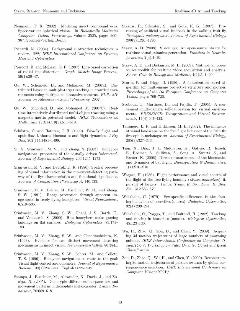
The general form of the apparatus is illustrated in Fig-ure 1A and a flowchart of operations is given in Figure 2A.Digital cameras are connected (with an IEEE 1394 FireWirebus or a dedicated gigabit ethernet cable) to image process-ing computers that perform a background subtraction basedalgorithm to extract image features such as the 2D target po-sition and orientation in a given camera’s image. From thesecomputers, this 2D information is transmitted over a gigabitethernet LAN to a central computer, which performs 2D-to-3D triangulation and tracking. Although the tracking resultsare generated and saved online, in realtime as the experimentis performed, raw image sequences can also be saved for bothverification purposes as well as other types of analyses. Fi-nally, reconstructed flight trajectories, such as that of Figure1B, may then be subjected to further analysis, as in Figures3 and 9.

(Figure 1 near here.)(Figure 2 near here.)(Figure 3 near here.)

1.2 Related Work

Several systems have allowed manual or manually-assisteddigitization of the trajectories of freely flying animals. In the1970s, Land and Collett performed pioneering studies on thevisual guidance of flight in blowflies (1974) and later, in hov-erflies (Collett and Land, 1975, 1978). By the end of the 70sand into the 80s, 3D reconstructions using two views of fly-ing insects were performed (Wehrhahn, 1979; Buelthoff et al.,1980; Wehrhahn et al., 1982; Dahmen and Zeil, 1984; Wagner,1986). In one case, the shadow of a bee on a planar white sur-face was used as a second view to perform 3D reconstruction(Srinivasan et al., 2000). Today, hand digitization is still usedwhen complex kinematics, such as wing shape and position,are desired, such as in Drosophila (Fry et al., 2003), cockatoo(Hedrick and Biewener, 2007) and bats (Tian et al., 2006).

Several authors have solved similar automated multi-targettracking problems using video. For example, Khan et al.(2005) tracked multiple, interacting ants in 2D from a sin-gle view using particle filtering with a Markov Chain MonteCarlo sampling step to solve the multi-target tracking prob-lem. Later work by the same authors (Khan et al., 2006)achieved realtime speeds through the use of sparse updat-ing techniques. Branson et al. (2009) addressed the sameproblem for walking flies. Their technique uses backgroundsubtraction and clustering to detect flies in the image, andcasts the data association problem as an instance of min-imum weight bipartite perfect matching. In implementingflydra, we found the simpler system described here to be suf-ficient for tracking position of flying flies and hummingbirds(see Section 5). In addition to tracking in three dimensionsrather than two, a key difference between the work describedabout and those addressed in the present work is that the in-teractions between our animals are relatively weak (see Sec-tion 3.2, especially equation 7), and we did not find it nec-essary to implement a more advanced tracker. Nevertheless,the present work could be used as the basis for a more ad-vanced tracker, such as one using a particle filter (e.g. Klein,2008). In that case, the posterior from the Extended KalmanFilter (see Section 3.1) could be used as the proposal distri-bution for the particle filter. Others have decentralized themultiple object tracking problem to improve performance, es-pecially when dealing with dynamic occlusions due to targetsoccluding each other (e.g. Qu et al., 2007a,b). Additionally,tracking of dense clouds of starlings (Ballerini et al., 2008;Cavagna et al., 2008c,b,a) and fruit flies (Wu et al., 2009; Zouet al., 2009) has enabled detailed investigation of swarms, al-though these systems are currently incapable of operating inrealtime. By filming inside a corner-cube reflector, multiple(real and reflected) images allowed Bomphrey et al. (2009) totrack flies in 3D with only a single camera, and the trackingalgorithm presented here could make use of this insight.

Completely automated 3D animal tracking systems havemore recently been created such as systems with two camerasthat track flies in realtime (Marden et al., 1997; Fry et al.,2004, 2008). The system of Grover et al. (2008), similar inmany respects to the one we describe here, tracks the visual

2


hull of flies using three cameras to reconstruct a polygonalmodel of the 3D shape of the flies. Our system, briefly de-scribed in a simpler, earlier form in Maimon et al. (2008), dif-fers in several ways. First, flydra has a design goal of trackingover large volumes, and, as a result of the associated limitedspatial resolution (rather than due to a lack of interest), fly-dra is concerned only with the location and orientation ofthe animal. Second, to facilitate tracking over large volumes,the flydra system uses a data association step as part of thetracking algorithm. The data association step allows flydra todeal with additional noise (false positive feature detections)when dealing with low contrast situations often present whenattempting to track in large volumes. Third, our system uti-lizes a general multi view geometry, whereas the system ofGrover et al. (2008) utilizes epipolar geometry, limiting itsuse to three cameras. Finally, although their system oper-ates in realtime, no measurements of latency were providedby Grover et al. (2008) with which to compare our measure-ments.

1.3 Notation

In the equations to follow, letters in a bold, roman font signifya vector, which may be specified by components enclosed inparentheses and separated by commas. Matrices are writtenin roman font with uppercase letters. Scalars are in italics.Vectors always act like a single column matrix, such that forvector v = (a, b, c), the multiplication with matrix M is Mv =

M[v]

= M

abc

.

2 2D feature extraction

The first stage of processing converts digital images into a listof feature points using an elaboration of a background sub-traction algorithm. Because the image of a target is usuallyonly a few pixels in area, an individual feature point from agiven camera characterizes that camera’s view of the target.In other words, neglecting missed detections or false positives,there is usually a one-to-one correspondence between targetsand extracted feature points from a given camera. Never-theless, our system is capable of successful tracking despitemissing observations due to occlusion or low contrast (seeSection 3.1) and rejecting false positive feature detections (asdescribed in Section 3.2).

In the Bayesian framework, all feature points for time t arethe observation Zt. The ith of n cameras returns m featurepoints, with each point zij being a vector zij = (u, v, α, β, θ, ε)where u and v are the coordinates of the point in the imageplane and the remaining components are local image statisticsdescribed below. Zt thus consists of all such feature points fora given frame Zt = {z11, . . . , z1m, . . . , zn1, . . . , znm}. (In theinterest of simplified notation, our indexing scheme is slightlymisleading here — there may be varying numbers of featuresfor each camera rather than always m as suggested.)

The process to convert a new image to a series of featurepoints uses a process based on background subtraction usingthe running Gaussian average method (reviewed in Piccardi,2004). To achieve fast image processing required for realtimeoperation, many of these operations are performed utilizingthe high-performance single instruction multiple data (SIMD)extensions available on recent x86 CPUs. Initially, an abso-lute difference image is made, where each pixel is the absolutevalue of the difference between the incoming frame and thebackground image. Feature points that exceed some thresh-old difference from the background image are noted and asmall region around each pixel is subjected to further anal-ysis. For the jth feature, the brightest point has value βjin this absolute difference image. All pixels below a certainfraction (e.g. 0.3) of βj are set to zero to reduce momentarms caused by spurious pixels. Feature area αj is foundfrom the 0th moment, the feature center (uj , vj) is calculatedfrom the 1st moment and the feature orientation θj and ec-centricity εj are calculated from higher moments. After cor-recting for lens distortion (see Section 4), the feature centeris (uj , vj). Thus, the jth point is characterized by the vec-tor zj = (uj , vj , αj , βj , θj , εj). Such features are extractedon every frame from every camera, although the number ofpoints m found on each frame may vary. We set the initialthresholds for detection low to minimize the number of misseddetections—false positives at this stage are rejected later bythe data association algorithm (Section 3.2).

Our system is capable of dealing with illumination condi-tions that vary slowly over time by using an ongoing esti-mate of the background luminance and its variance, whichare maintained on a per-pixel basis by updating the currentestimates with data from every 500th frame (or other arbi-trary interval). A more sophisticated 2D feature extractionalgorithm could be used, but we have found this scheme to besufficient for our purposes and sufficiently simple to operatewith minimal latency.

While the realtime operation of flydra is essential for ex-periments modifying sensory feedback, another advantage ofan online tracking system is that the amount of data requiredto be saved for later analysis is greatly reduced. By perform-ing only 2D feature extraction in realtime, to reconstruct 3Dtrajectories later, only the vectors zj need be saved, resultingin orders of magnitude less data than the full-frame cameraimages. Thus, to achieve solely the low data rates of real-time tracking, the following sections dealing with 3D are notnecessary to be implemented for this benefit of realtime use.Furthermore, raw images taken from the neighborhood of thefeature points could also be extracted and saved for later anal-ysis, saving slightly more data, but still at rates substantiallyless than the full camera frames provide. This fact is partic-ularly useful for cameras with a higher data rate than harddrives can save, and such a feature is implemented in flydra.

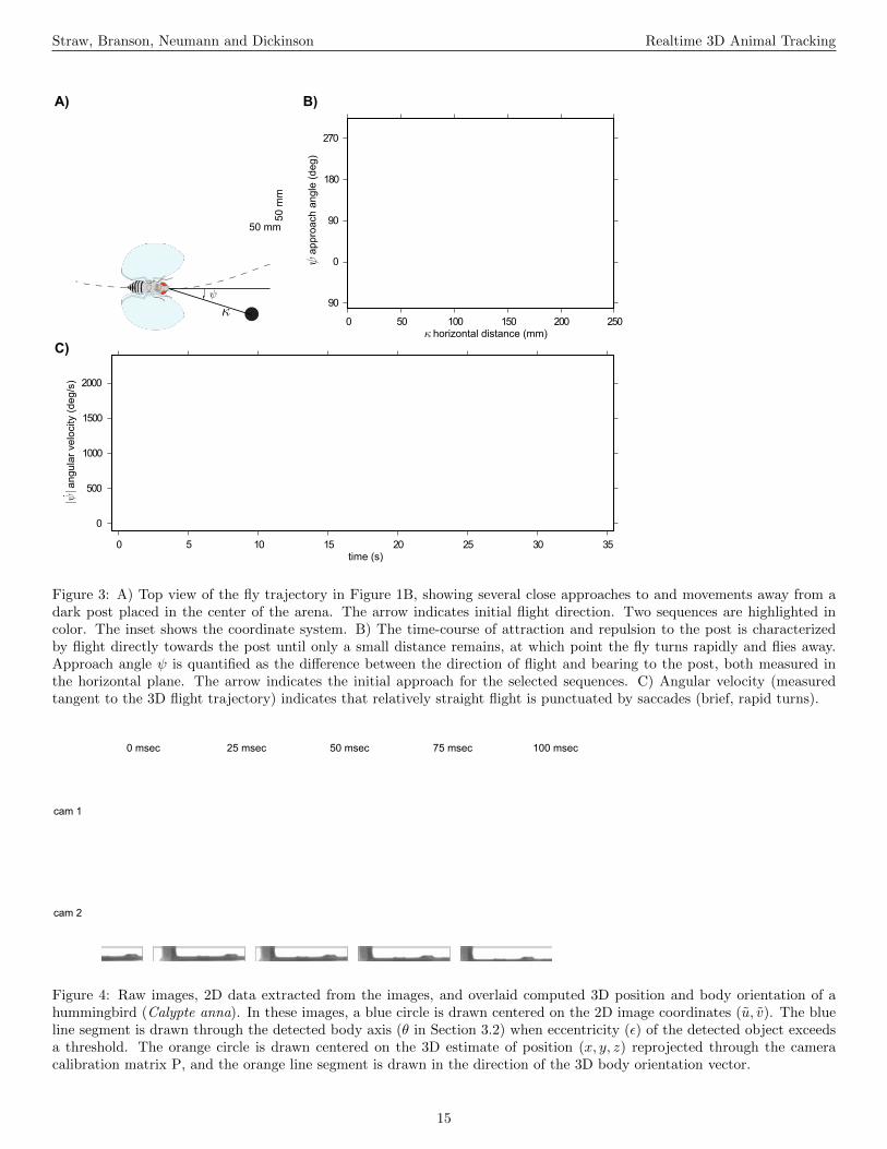
(Figure 4 near here.)Figure 4 shows the parameters (u, v, θ) from the 2D feature

extraction algorithm during a hummingbird flight. These 2Dfeatures, in addition to 3D reconstructions, are overlaid onraw images extracted and saved using the realtime image ex-

3


traction technique described above.

3 Multi target tracking

The goal of flydra, as described in Section 1.1, is to find theMAP estimate of the state of all targets. For simplicity, wemodel interaction between targets in a very limited way. Al-though in many cases the animals we are interested in track-ing do interact (for example, hummingbirds engage in com-petition in which they threaten or even contact each other),mathematically limiting the interaction facilitates a reductionin computational complexity. First, the process update is in-dependent for each kth animal

p(St|St−1) =∏k

p(St,k|St−1,k). (2)

Second, we implemented only a slight coupling between tar-gets in the data association algorithm. Thus, the observationlikelihood model p(Zt|St) is independent for each target withthe exception described in Section 3.2.1, and making this as-sumption allows use of the Nearest Neighbor Standard Filteras described below.

Modeling individual target states as mostly independent al-lows the problem of estimating the MAP of joint target stateS to be treated nearly as l independent, smaller problems.One benefit of making the assumption of target independenceis that the target tracking and data association parts of oursystem are parallelizable. Although not yet implemented inparallel, our system is theoretically capable of tracking verymany (tens or hundreds) targets simultaneously with low la-tency on a computer with sufficiently many processing units.

The cost of this near-indepdence assumption is reducedtracking accuracy during periods of near contact (see Sec-ton 3.2.1). Data from these periods could be analyzed laterusing more sophisticated multi-target tracking data associa-tion techniques, presumably in an offline setting, especiallybecause such periods could be easily identified using a sim-ple algorithm. All data presented in this paper utilized theprocedure described here.

3.1 Kalman filtering

The standard Extended Kalman Filter (EKF) approximatelyestimates statistics of the posterior distribution (equation 1)for non-linear processes with additive Gaussian noise (detailsare given in Appendix A). To utilize this framework, we makethe assumption that noise in the relevant processes is Gaus-sian. Additionally, our target independence assumption al-lows a single Kalman filter implementation to be used for eachtracked target. The EKF estimates state and its covariancebased on a prior state estimate and incoming observationsby using models of the state update process, the observationprocess, and estimates of the noise of each process.

We use a linear model for the dynamics of the system anda nonlinear model of the observation process. Specifically,

the time evolution of the system is modeled with the lineardiscrete stochastic model

st = Ast−1 + w. (3)

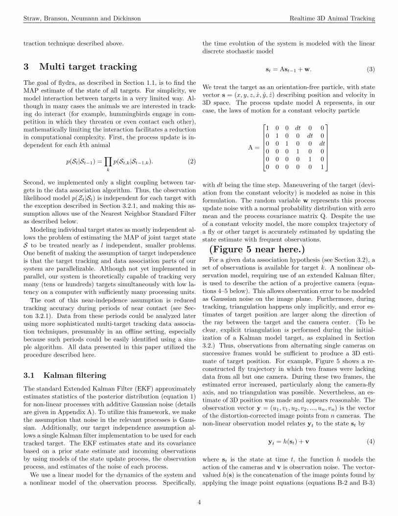
We treat the target as an orientation-free particle, with statevector s = (x, y, z, x, y, z) describing position and velocity in3D space. The process update model A represents, in ourcase, the laws of motion for a constant velocity particle

A =

1 0 0 dt 0 00 1 0 0 dt 00 0 1 0 0 dt0 0 0 1 0 00 0 0 0 1 00 0 0 0 0 1

with dt being the time step. Maneuvering of the target (devi-ation from the constant velocity) is modeled as noise in thisformulation. The random variable w represents this processupdate noise with a normal probability distribution with zeromean and the process covariance matrix Q. Despite the useof a constant velocity model, the more complex trajectory ofa fly or other target is accurately estimated by updating thestate estimate with frequent observations.

(Figure 5 near here.)For a given data association hypothesis (see Section 3.2), a

set of observations is available for target k. A nonlinear ob-servation model, requiring use of an extended Kalman filter,is used to describe the action of a projective camera (equa-tions 4–5 below). This allows observation error to be modeledas Gaussian noise on the image plane. Furthermore, duringtracking, triangulation happens only implicitly, and error es-timates of target position are larger along the direction ofthe ray between the target and the camera center. (To beclear, explicit triangulation is performed during the initial-ization of a Kalman model target, as explained in Section3.2.) Thus, observations from alternating single cameras onsuccessive frames would be sufficient to produce a 3D esti-mate of target position. For example, Figure 5 shows a re-constructed fly trajectory in which two frames were lackingdata from all but one camera. During these two frames, theestimated error increased, particularly along the camera-flyaxis, and no triangulation was possible. Nevertheless, an es-timate of 3D position was made and appears reasonable. Theobservation vector y = (u1, v1, u2, v2, ..., un, vn) is the vectorof the distortion-corrected image points from n cameras. Thenon-linear observation model relates yt to the state st by

yt = h(st) + v (4)

where st is the state at time t, the function h models theaction of the cameras and v is observation noise. The vector-valued h(s) is the concatenation of the image points found byapplying the image point equations (equations B-2 and B-3)

4


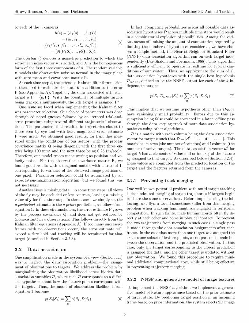
to each of the n cameras

h(s) = (h1(s), ..., hn(s))

= (u1, v1, ..., un, vn)

= (r1/t1, s1/t1, ..., rn/tn, sn/tn)

= (H(P1X), ...,H(PnX)).

(5)

The overbar () denotes a noise-free prediction to which thezero-mean noise vector v is added, and X is the homogeneousform of the first three components of s. The random variablev models the observation noise as normal in the image planewith zero mean and covariance matrix R.

At each time step t, the extended Kalman filter formulationis then used to estimate the state s in addition to the errorP (see Appendix A). Together, the data associated with eachtarget is Γ = {s,P}. With the possibility of multiple targetsbeing tracked simultaneously, the kth target is assigned Γk.

One issue we faced when implementing the Kalman filterwas parameter selection. Our choice of parameters was donethrough educated guesses followed by an iterated trial-and-error procedure using several different trajectories’ observa-tions. The parameters that resulted in trajectories closest tothose seen by eye and with least magnitude error estimateP were used. We obtained good results, for fruit flies mea-sured under the conditions of our setups, with the processcovariance matrix Q being diagonal, with the first three en-tries being 100 mm2 and the next three being 0.25 (m/sec)2.Therefore, our model treats maneuvering as position and ve-locity noise. For the observation covariance matrix R, wefound good results with a diagonal matrix with entries of 1,corresponding to variance of the observed image positions ofone pixel. Parameter selection could be automated by anexpectation-maximization algorithm, but we found this wasnot necessary.

Another issue is missing data—in some time steps, all viewsof the fly may be occluded or low contrast, leaving a missingvalue of y for that time step. In those cases, we simply set thea posteriori estimate to the a priori prediction, as follows fromequation 1. In these circumstances, the error estimate P growsby the process covariance Q, and does not get reduced by(nonexistant) new observations. This follows directly from theKalman filter equations (Appendix A). If too many successiveframes with no observations occur, the error estimate willexceed a threshold and tracking will be terminated for thattarget (described in Section 3.2.3).

3.2 Data association

One simplification made in the system overview (Section 1.1)was to neglect the data association problem—the assign-ment of observations to targets. We address the problem bymarginalizing the observation likelihood across hidden dataassociation variables D, where each D corresponds to a differ-ent hypothesis about how the feature points correspond withthe targets. Thus, the model of observation likelihood fromequation 1 becomes

p(Zt|St) =∑Dp(Zt,D|St). (6)

In fact, computing probabilities across all possible data as-sociation hypothesesD across multiple time steps would resultin a combinatorial explosion of possibilities. Among the vari-ous means of limiting the amount of computation required bylimiting the number of hypotheses considered, we have cho-sen a simple method, the Nearest Neighbor Standard Filter(NNSF) data association algorithm run on each target inde-pendently (Bar-Shalom and Fortmann, 1988). This algorithmis sufficiently efficient to operate in realtime for typical con-ditions of our system. Thus, we approximate the sum of alldata association hypotheses with the single best hypothesisDNNSF, defined to be the NNSF output for each of the k in-dependent targets

p(Zt,DNNSF|St) ≈∑Dp(Zt,D|St). (7)

This implies that we assume hypotheses other than DNNSF

have vanishingly small probability. Errors due to this as-sumption being false could be corrected in a later, offline passthrough the data keeping track of more data association hy-potheses using other algorithms.

D is a matrix with each column being the data associationvector for target k such that D = [d1 . . . dk . . . ]. Thismatrix has n rows (the number of cameras) and l columns (thenumber of active targets). The data association vector dk fortarget k has n elements of value null or index j of the featurezj assigned to that target. As described below (Section 3.2.4),these values are computed from the predicted location of thetarget and the features returned from the cameras.

3.2.1 Preventing track merging

One well known potential problem with multi target trackingis the undesired merging of target trajectories if targets beginto share the same observations. Before implementing the fol-lowing rule, flydra would sometimes suffer from this mergingproblem when tracking hummingbirds engaged in territorialcompetition. In such fights, male hummingbirds often fly di-rectly at each other and come in physical contact. To preventthe two trajectories from merging in such cases, a single passis made through the data association assignments after eachframe. In the case that more than one target was assigned theexact same subset of feature points, a comparison is made be-tween the observation and the predicted observation. In thiscase, only the target corresponding to the closest predictionis assigned the data, and the other target is updated withoutany observation. We found this procedure to require mini-mal additional computational cost, while still being effectivein preventing trajectory merging.

3.2.2 NNSF and generative model of image features

To implement the NNSF algorithm, we implement a genera-tive model of feature appearance based on the prior estimateof target state. By predicting target position in an incomingframe based on prior information, the system selects 2D image

5


points as being likely to come from the target by gating un-likely observations, thus limiting the amount of computationperformed.

(Figure 6 near here.)Recall from Section 2 that for each time t and camera i,

m feature points are found with the jth point being zj =(uj , vj , αj , βj , θj , εj). The distortion-corrected image coordi-nates are (u, v), while α is the area of the object on the imageplane measured by thresholding of the difference image be-tween the current and background image, β is an estimateof the maximum difference within the difference image, andθ and ε are the slope and eccentricity of the image feature.Each camera may return multiple candidate points per timestep, with all points from the ith camera represented as Zi,a matrix whose columns are the individual vectors zj , suchthat Zi =

[z1 ... zm

]. The purpose of the data association

algorithm is to assign each incoming point z to an existingKalman model Γ, to initialize a new Kalman model, or at-tribute it to a false positive (a null target). Furthermore, oldKalman models for which no recent observations exist dueto the target leaving the tracking volume must be deleted.The use of such a data association algorithm allows flydra totrack multiple targets simultaneously, as in Figure 6, and, byreducing computational costs, allows the 2D feature extrac-tion algorithm to return many points to minimize the numberof missed detections.

3.2.3 Entry and exit of targets

How does our system deal with existing targets losing visibil-ity due to leaving the tracking volume, occlusion or loweredvisual contrast? What happens when new targets become vis-ible? We treat such occurrences as part of the update modelin the Bayesian framework of Section 1.1. Thus, in the ter-minology from that section, our motion model for all targetsp(St|St−1) includes the possibility of initializing a new targetor removing an existing target. This section describes theprocedure followed.

For all data points z that remained ‘unclaimed’ by the pre-dicted locations of pre-existing targets (see Section 3.2.4 be-low), we use an unguided hypothesis testing algorithm. Thistriangulates a hypothesized 3D point for every possible com-bination of 2,3,...,n cameras, for a total of

(n2

)+(n3

)+ ...

+(nn

)combinations. Any 3D point with reprojection error

less than an arbitrary threshold using the greatest numberof cameras is then used to initialize a new Kalman filter in-stance. The initial state estimate is set to that 3D positionwith zero velocity and a relatively high error estimate. Track-ing is stopped (a target is removed) once the estimated errorP exceeds a threshold. This most commonly happens, forexample, when the target leaves the tracking area and thusreceives no observations for a given number of frames.

3.2.4 Using incoming data

Ultimately, the purpose of the data association step is to de-termine which image feature points will be used by which

target. Given the target independence assumption, each tar-get uses incoming data independently. This section outlineshow the data association algorithm is used to determine thefeature points treated as the observation for a given target.

To utilize the Kalman filter described in Section 3.1, obser-vation vectors must be formed from the incoming data. Falsepositives must be separated from correct detections, and, be-cause multiple targets may be tracked simultaneously, cor-rect detections must be associated with a particular Kalmanmodel. At the beginning of processing for each time step tfor the kth Kalman model, a prior estimate of target positionand error Γk

t|t−1 = {skt|t−1,Pkt|t−1} is available. It must be

determined which, if any, of the m image points from the ithcamera is associated with the kth target. Due to the realtimerequirements for our system, flydra gates incoming detectionson simple criteria before performing more computationallyintensive tasks.

For target k at time t, the data association function g is

dkt = g(Z1, ...,Zn, Γk

t|t−1). (8)

This is a function of the image points Zi from each of the ncameras and the prior information for target k. The assign-ment vector for the kth target, dk, defines which points fromwhich cameras view a target. This vector has a componentfor each of the n cameras, which is either null (if that cameradoesn’t contribute) or is the column index of Zi correspondingto the associated point. Thus, dk has length n, the numberof cameras, and no camera may view the same target morethan once. Note, the k and t superscript and subscript on dindicate the assignment vector is for target k at time step t,whereas below (Equation 9), the subscript i is used to indicatethe ith component of the vector d.

The data association function g may be written in terms ofthe components of d. The ith component is the index of thecolumns of Zi that maximizes likelihood of the observationgiven the predicted target state and error and is defined to be

di = argmaxj

(p(zj |Γ)), zj ∈ Zi. (9)

Our likelihood function gates detections based on two condi-tions. First, the incoming detected location (uj , vj) must bewithin a threshold Euclidean distance from the estimated tar-get location projected on the image. The Euclidean distanceon the image plane is

dist2d = deuclid(

[ujvj

],H(PiX)) (10)

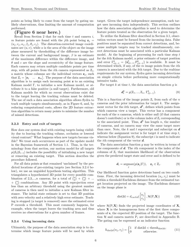
where H(PiX) finds the projected image coordinates of X,where X is the homogeneous form of the first three compo-nents of s, the expected 3D position of the target. The func-tion H and camera matrix Pi are described in Appendix B.The gating can be expressed as an indicator function

1dist2d(uj , vj) =

{1 if dist2d < threshdist2d,0 otherwise.

(11)

6


Second, the area of the detected object (αj) must be greaterthan a threshold value, expressed as

1area(αj) =

{1 if αj > thresharea,0 otherwise.

(12)

If these conditions are met, the distance of the ray connectingthe camera center and 2D point on the image plane (uj , vj)from the expected 3D location a is used to further determinelikelihood. We use the Mahalanobis distance, which for avector a with an expected value of a with covariance matrixΣ is

dmahal(a, a) =√

(a− a)TΣ−1(a− a). (13)

Because the distance function is convex for a given a and Σ,we can solve directly for the closest point on the ray, by settinga equal to the first three terms of st|t−1 and Σ to the upper left3× 3 submatrix of Pt|t−1. Then, if the ray is a parametrizedline of the form L(s) = s · (a, b, c) + (x, y, z) where (a, b, c) isthe direction of the ray formed by the image point (u, v) andthe camera center and (x, y, z) is a point on the ray, we canfind the value of s for which the distance between L(s) anda is minimized by finding the value of s where derivative ofdmahal(L(s), a) is zero. If we call this closest point a andcombine equations 11–13, then our likelihood function is

p(zj |Γ) = 1dist2d(uj , vj) 1area(αj) e−dmahal(a,a) . (14)

Note that, due to the multiplication, if either of the first twofactors are zero, the third (and more computationally expen-sive) condition need not be evaluated.

4 Camera and lens calibration

Camera calibrations may be obtained in any way that pro-duces camera calibration matrices (described in Appendix B)and, optionally, parameters for a model of the non-linear dis-tortions of cameras. Good calibrations are critical for flydrabecause, as target visibility changes from one subset of cam-eras to another subset, any misalignment of the calibrationswill introduce artifactual movement in the reconstructed tra-jectories. Typically, we obtain camera calibrations in a twostep process. First, the Direct Linear Transformation (DLT)algorithm (Abdel-Aziz and Karara, 1971) directly estimatescamera calibration matrices Pi that could be used for triangu-lation as described in Appendix B. However, because we useonly about 10 manually digitized corresponding 2D/3D pairsper camera, this calibration is relatively low-precision and, asperformed, ignores optical distortions causing deviations fromthe linear simple pinhole camera model. Therefore, an auto-mated Multi-Camera Self Calibration Toolbox (Svoboda et al.,2005) is used as a second step. This toolbox utilizes inher-ent numerical redundancy when multiple cameras are view-ing a common set of 3D points through use of a factorizationalgorithm (Sturm and Triggs, 1996) followed by bundle ad-justment (reviewed in Section 18.1 of Hartley and Zisserman,2003). By moving a small LED point light source throughthe tracking volume (or, indeed, a freely flying fly), hundreds

of corresponding 2D/3D points are generated which lead toa single, overdetermined solution which, without knowing the3D positions of the LED, is accurate up to a scale, rotation,and translation. The camera centers, either from the DLTalgorithm or measured directly, are then used to find the bestscale, rotation, and translation. As part of the Multi-CameraSelf Calibration Toolbox, this process may be iterated withan additional step to estimate non-linear camera parameterssuch as radial distortion (Svoboda et al., 2005) using the Cam-era Calibration Toolbox of Bouguet. Alternatively, we havealso implemented the method of Prescott and McLean (1997)to estimate radial distortion parameters before use of Svo-boda’s toolbox, which we found necessary when using wideangle lenses with significant radial distortion (e.g. 150 pixelsin some cases).

5 Implementation and evaluation

We built three different flydra systems: a five camera, sixcomputer 100 fps system for tracking fruit flies in a 0.3mx 0.3m x 1.5m arena (e.g. Figures 1, 9 and Maimon et al.2008, which used the same hardware but a simpler version ofthe tracking software), an eleven camera, nine computer 60fps system for tracking fruit flies in a large—2m diameter x0.8m high—cylinder (e.g. Figure 5) and a four camera, fivecomputer 200 fps system for tracking hummingbirds in a 1.5mx 1.5m x 3m arena (e.g. Figure 4). Apart from the low-levelcamera drivers, the same software is running on each of thesesystems.

We used the Python computer language to implement fly-dra. Several other pieces of software, most of which are opensource, are instrumental to this system: motmot (Straw andDickinson, 2009), pinpoint, pytables, numpy, scipy, Pyro, wx-Python, tvtk, VTK, matplotlib, PyOpenGL, pyglet, Pyrex,cython, ctypes, Intel IPP, ATLAS, libdc1394, PTPd, gcc, andUbuntu. We used Intel Pentium 4 and Core 2 Duo based com-puters.

The accuracy of 3D reconstructions was verified in twoways. First, the distance between 2D points projected from a3D estimate derived from the originally extracted 2D pointsis a measure of calibration accuracy. For all figures shown,the mean reprojection error was less than one pixel, and formost cameras in most figures, was less than 0.5 pixels. Sec-ondly, the 3D coordinates and distances between coordinatesmeasured through triangulation were verified against valuesmeasured physically. For two such measurements in the sys-tem shown in Figure 1, these values were within 4 percent.

(Figure 7 near here.)We measured the latency of the 3D reconstruction by syn-

chronizing several clocks involved in our experimental setupand then measuring the duration between onset of image ac-quisition and completion of the computation of target posi-tion. When flydra is running, the clocks of the various com-puters are synchronized to within 1 microsecond by PTPd, theprecise time protocol daemon, an implementation of the IEEE1588 clock synchronization protocol (Correll et al., 2005). Ad-

7


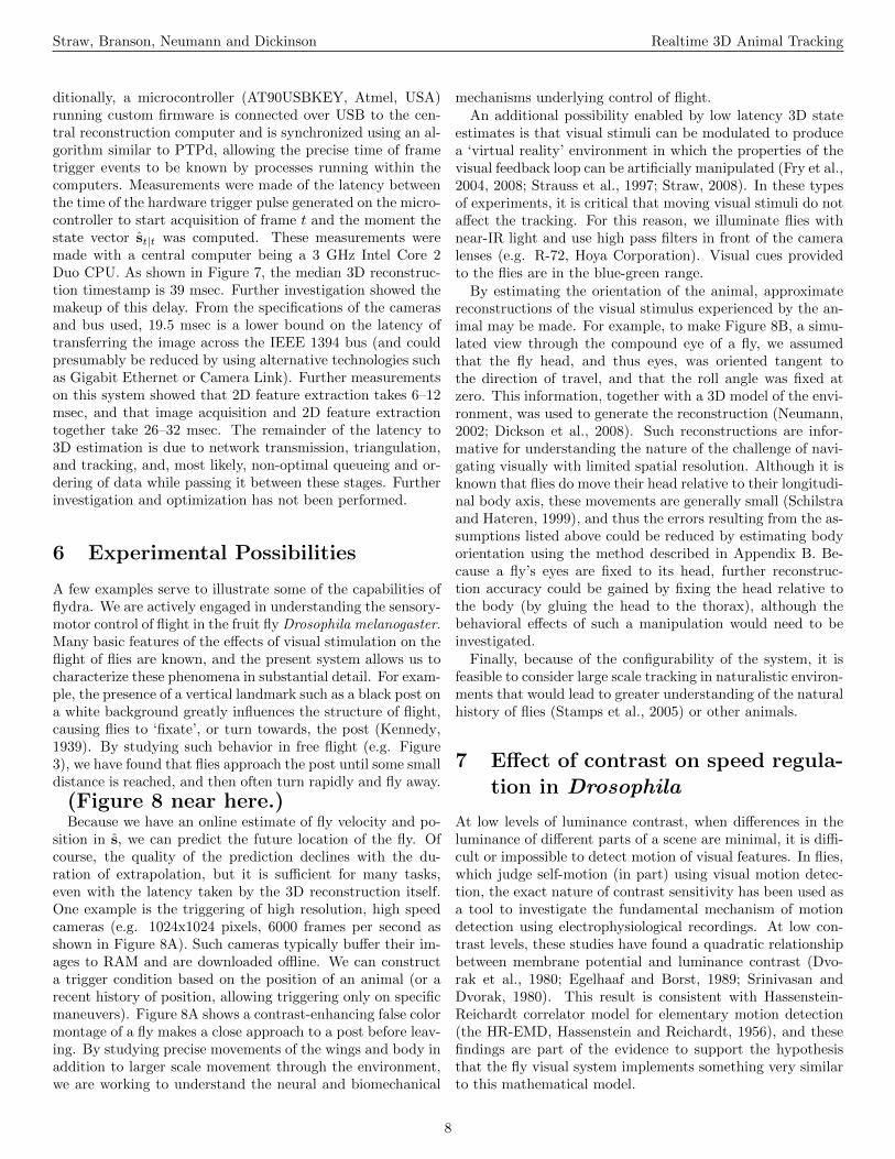
ditionally, a microcontroller (AT90USBKEY, Atmel, USA)running custom firmware is connected over USB to the cen-tral reconstruction computer and is synchronized using an al-gorithm similar to PTPd, allowing the precise time of frametrigger events to be known by processes running within thecomputers. Measurements were made of the latency betweenthe time of the hardware trigger pulse generated on the micro-controller to start acquisition of frame t and the moment thestate vector st|t was computed. These measurements weremade with a central computer being a 3 GHz Intel Core 2Duo CPU. As shown in Figure 7, the median 3D reconstruc-tion timestamp is 39 msec. Further investigation showed themakeup of this delay. From the specifications of the camerasand bus used, 19.5 msec is a lower bound on the latency oftransferring the image across the IEEE 1394 bus (and couldpresumably be reduced by using alternative technologies suchas Gigabit Ethernet or Camera Link). Further measurementson this system showed that 2D feature extraction takes 6–12msec, and that image acquisition and 2D feature extractiontogether take 26–32 msec. The remainder of the latency to3D estimation is due to network transmission, triangulation,and tracking, and, most likely, non-optimal queueing and or-dering of data while passing it between these stages. Furtherinvestigation and optimization has not been performed.

6 Experimental Possibilities

A few examples serve to illustrate some of the capabilities offlydra. We are actively engaged in understanding the sensory-motor control of flight in the fruit fly Drosophila melanogaster.Many basic features of the effects of visual stimulation on theflight of flies are known, and the present system allows us tocharacterize these phenomena in substantial detail. For exam-ple, the presence of a vertical landmark such as a black post ona white background greatly influences the structure of flight,causing flies to ‘fixate’, or turn towards, the post (Kennedy,1939). By studying such behavior in free flight (e.g. Figure3), we have found that flies approach the post until some smalldistance is reached, and then often turn rapidly and fly away.

(Figure 8 near here.)Because we have an online estimate of fly velocity and po-

sition in s, we can predict the future location of the fly. Ofcourse, the quality of the prediction declines with the du-ration of extrapolation, but it is sufficient for many tasks,even with the latency taken by the 3D reconstruction itself.One example is the triggering of high resolution, high speedcameras (e.g. 1024x1024 pixels, 6000 frames per second asshown in Figure 8A). Such cameras typically buffer their im-ages to RAM and are downloaded offline. We can constructa trigger condition based on the position of an animal (or arecent history of position, allowing triggering only on specificmaneuvers). Figure 8A shows a contrast-enhancing false colormontage of a fly makes a close approach to a post before leav-ing. By studying precise movements of the wings and body inaddition to larger scale movement through the environment,we are working to understand the neural and biomechanical

mechanisms underlying control of flight.An additional possibility enabled by low latency 3D state

estimates is that visual stimuli can be modulated to producea ‘virtual reality’ environment in which the properties of thevisual feedback loop can be artificially manipulated (Fry et al.,2004, 2008; Strauss et al., 1997; Straw, 2008). In these typesof experiments, it is critical that moving visual stimuli do notaffect the tracking. For this reason, we illuminate flies withnear-IR light and use high pass filters in front of the cameralenses (e.g. R-72, Hoya Corporation). Visual cues providedto the flies are in the blue-green range.

By estimating the orientation of the animal, approximatereconstructions of the visual stimulus experienced by the an-imal may be made. For example, to make Figure 8B, a simu-lated view through the compound eye of a fly, we assumedthat the fly head, and thus eyes, was oriented tangent tothe direction of travel, and that the roll angle was fixed atzero. This information, together with a 3D model of the envi-ronment, was used to generate the reconstruction (Neumann,2002; Dickson et al., 2008). Such reconstructions are infor-mative for understanding the nature of the challenge of navi-gating visually with limited spatial resolution. Although it isknown that flies do move their head relative to their longitudi-nal body axis, these movements are generally small (Schilstraand Hateren, 1999), and thus the errors resulting from the as-sumptions listed above could be reduced by estimating bodyorientation using the method described in Appendix B. Be-cause a fly’s eyes are fixed to its head, further reconstruc-tion accuracy could be gained by fixing the head relative tothe body (by gluing the head to the thorax), although thebehavioral effects of such a manipulation would need to beinvestigated.

Finally, because of the configurability of the system, it isfeasible to consider large scale tracking in naturalistic environ-ments that would lead to greater understanding of the naturalhistory of flies (Stamps et al., 2005) or other animals.

7 Effect of contrast on speed regula-tion in Drosophila

At low levels of luminance contrast, when differences in theluminance of different parts of a scene are minimal, it is diffi-cult or impossible to detect motion of visual features. In flies,which judge self-motion (in part) using visual motion detec-tion, the exact nature of contrast sensitivity has been used asa tool to investigate the fundamental mechanism of motiondetection using electrophysiological recordings. At low con-trast levels, these studies have found a quadratic relationshipbetween membrane potential and luminance contrast (Dvo-rak et al., 1980; Egelhaaf and Borst, 1989; Srinivasan andDvorak, 1980). This result is consistent with Hassenstein-Reichardt correlator model for elementary motion detection(the HR-EMD, Hassenstein and Reichardt, 1956), and thesefindings are part of the evidence to support the hypothesisthat the fly visual system implements something very similarto this mathematical model.

8


Despite these and other electrophysiological findings sug-gesting the HR-EMD may underlie fly motion sensitivity,studies of flight speed regulation and other visual behaviorsin freely flying flies (David, 1982) and honey bees (Srinivasanet al., 1991; Si et al., 2003; Srinivasan et al., 1993) show thatthe free-flight behavior of these insects is inconsistent with aflight velocity regulator based on a simple HR-EMD model.More recently, Baird et al. (2005) have shown that over alarge range of contrasts, flight velocity in honey bees is nearlyunaffected by contrast. As noted by those authors, however,their setup was unable to achieve true zero contrast due to im-perfections with their apparatus. They suggest that contrastadaptation (Harris et al., 2000) may have been responsiblefor boosting the responses to low contrasts and attenuatingresponses to high contrast. This possibility was supportedby the finding that forward velocity was better regulated atthe nominal “zero contrast” condition than in the presence ofan axial stripe, which may have had the effect of preventingcontrast adaptation while provide no contrast perpendicularto the direction of flight (Baird et al., 2005).

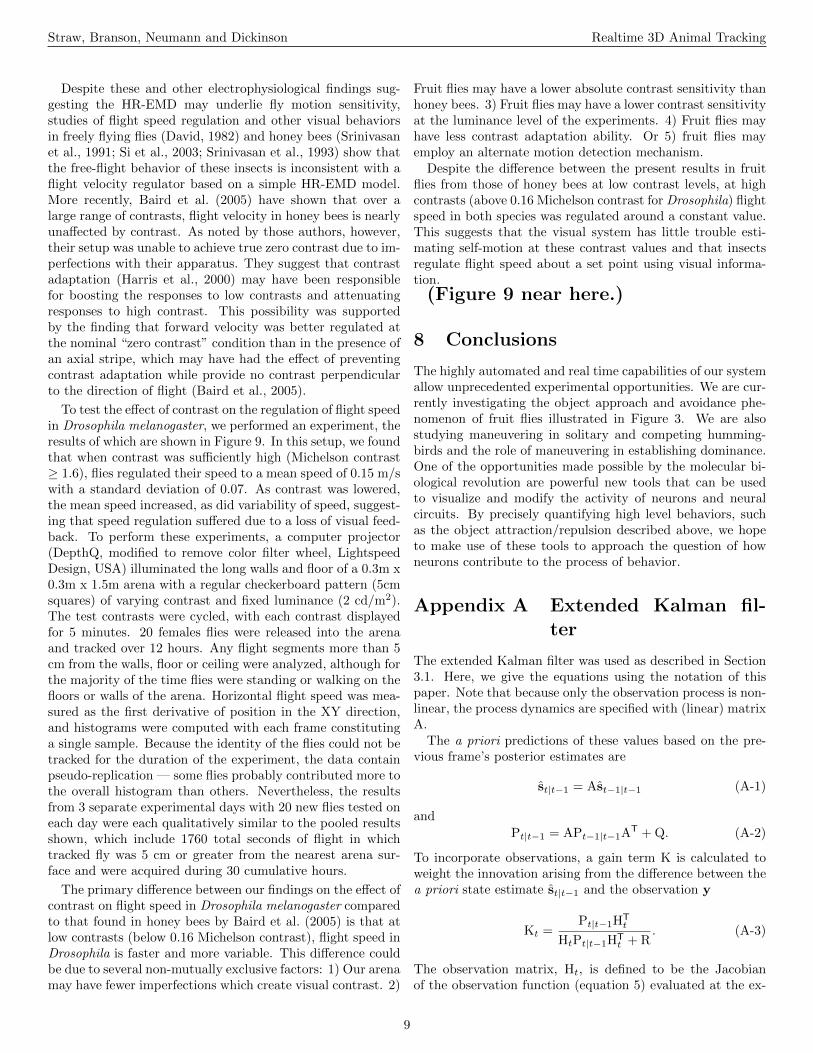
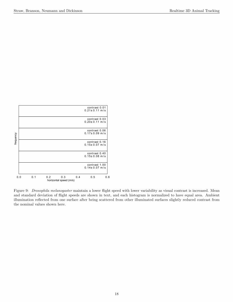
To test the effect of contrast on the regulation of flight speedin Drosophila melanogaster, we performed an experiment, theresults of which are shown in Figure 9. In this setup, we foundthat when contrast was sufficiently high (Michelson contrast≥ 1.6), flies regulated their speed to a mean speed of 0.15 m/swith a standard deviation of 0.07. As contrast was lowered,the mean speed increased, as did variability of speed, suggest-ing that speed regulation suffered due to a loss of visual feed-back. To perform these experiments, a computer projector(DepthQ, modified to remove color filter wheel, LightspeedDesign, USA) illuminated the long walls and floor of a 0.3m x0.3m x 1.5m arena with a regular checkerboard pattern (5cmsquares) of varying contrast and fixed luminance (2 cd/m2).The test contrasts were cycled, with each contrast displayedfor 5 minutes. 20 females flies were released into the arenaand tracked over 12 hours. Any flight segments more than 5cm from the walls, floor or ceiling were analyzed, although forthe majority of the time flies were standing or walking on thefloors or walls of the arena. Horizontal flight speed was mea-sured as the first derivative of position in the XY direction,and histograms were computed with each frame constitutinga single sample. Because the identity of the flies could not betracked for the duration of the experiment, the data containpseudo-replication — some flies probably contributed more tothe overall histogram than others. Nevertheless, the resultsfrom 3 separate experimental days with 20 new flies tested oneach day were each qualitatively similar to the pooled resultsshown, which include 1760 total seconds of flight in whichtracked fly was 5 cm or greater from the nearest arena sur-face and were acquired during 30 cumulative hours.

The primary difference between our findings on the effect ofcontrast on flight speed in Drosophila melanogaster comparedto that found in honey bees by Baird et al. (2005) is that atlow contrasts (below 0.16 Michelson contrast), flight speed inDrosophila is faster and more variable. This difference couldbe due to several non-mutually exclusive factors: 1) Our arenamay have fewer imperfections which create visual contrast. 2)

Fruit flies may have a lower absolute contrast sensitivity thanhoney bees. 3) Fruit flies may have a lower contrast sensitivityat the luminance level of the experiments. 4) Fruit flies mayhave less contrast adaptation ability. Or 5) fruit flies mayemploy an alternate motion detection mechanism.

Despite the difference between the present results in fruitflies from those of honey bees at low contrast levels, at highcontrasts (above 0.16 Michelson contrast for Drosophila) flightspeed in both species was regulated around a constant value.This suggests that the visual system has little trouble esti-mating self-motion at these contrast values and that insectsregulate flight speed about a set point using visual informa-tion.

(Figure 9 near here.)

8 Conclusions

The highly automated and real time capabilities of our systemallow unprecedented experimental opportunities. We are cur-rently investigating the object approach and avoidance phe-nomenon of fruit flies illustrated in Figure 3. We are alsostudying maneuvering in solitary and competing humming-birds and the role of maneuvering in establishing dominance.One of the opportunities made possible by the molecular bi-ological revolution are powerful new tools that can be usedto visualize and modify the activity of neurons and neuralcircuits. By precisely quantifying high level behaviors, suchas the object attraction/repulsion described above, we hopeto make use of these tools to approach the question of howneurons contribute to the process of behavior.

Appendix A Extended Kalman fil-ter

The extended Kalman filter was used as described in Section3.1. Here, we give the equations using the notation of thispaper. Note that because only the observation process is non-linear, the process dynamics are specified with (linear) matrixA.

The a priori predictions of these values based on the pre-vious frame’s posterior estimates are

st|t−1 = Ast−1|t−1 (A-1)

and

Pt|t−1 = APt−1|t−1AT + Q. (A-2)

To incorporate observations, a gain term K is calculated toweight the innovation arising from the difference between thea priori state estimate st|t−1 and the observation y

Kt =Pt|t−1HT

t

HtPt|t−1HTt + R

. (A-3)

The observation matrix, Ht, is defined to be the Jacobianof the observation function (equation 5) evaluated at the ex-

9


pected state

Ht =∂h

∂s

∣∣∣∣st|t−1

. (A-4)

The posterior estimates are then

st|t = st|t−1 + Kt(yt −Htst|t−1) (A-5)

and

Pt|t = (I−KtHt)Pt|t−1. (A-6)

Appendix B Triangulation

The basic 2D-to-3D calculation finds the best 3D location fortwo or more 2D camera views of a point, and is implementedusing a linear least-squares fit of the intersection of n raysdefined by the 2D image points and 3D camera centers ofeach of the n cameras (Hartley and Zisserman, 2003). Aftercorrection for radial distortion, the image of a 3D point onthe ith camera is (ui, vi). For mathematical reasons, it isconvenient to represent this 2D image point in homogeneouscoordinates

xi = (ri, si, ti), (B-1)

such that ui = ri/ti and vi = si/ti. For convenience, we definethe function H to convert from homogeneous to Cartesiancoordinates, thus

H(x) = (u, v) = (r/t, s/t). (B-2)

The 3 × 4 camera calibration matrix Pi models the projec-tion from a 3D homogeneous point X = (X1, X2, X3, X4)(representing the 3D point with inhomogeneous coordinates(x, y, z) = (X1/X4, X2/X4, X3/X4)) into the image point:

xi = PiX. (B-3)

By combining the image point equation B-3 from two or morecameras, we can solve for X using the homogeneous lineartriangulation method based on the singular value decompo-sition as described in Hartley and Zisserman (2003, Sections12.2 and A5.3).

A similar approach can be used for reconstructing the ori-entation of the longitudinal axis of an insect or bird. Briefly,a line is fit to this axis in each 2D image (using u, v and θfrom Section 2) and, together with the camera center, is usedto represent a plane in 3D space. The best-fit line of inter-section of the n planes is then found with a similar singularvalue decomposition algorithm (Hartley and Zisserman, 2003,Section 12.7).

Acknowledgments

The data for Figure 4 were gathered in collaboration withDouglas Altshuler. Sawyer Fuller helped with the EKF for-mulation, provided helpful feedback on the manuscript and,together with Gaby Maimon, Rosalyn Sayaman, Martin Peek

and Aza Raskin, helped with physical construction of are-nas and bug reports on the software. Pete Trautmann pro-vided insight on data association, and Pietro Perona pro-vided helpful suggestions on the manuscript. This work wassupported by grants from the Packard Foundation, AFOSR(FA9550-06-1-0079), ARO (DAAD 19-03-D-0004) and NIH(R01 DA022777).

References

Abdel-Aziz, Y. I. and Karara, H. M. (1971). Direct lineartransformation from comparator coordinates into objectspace coordinates. American Society of PhotogrammetrySymposium on Close-Range Photogrammetry, pages 1–18.

Baird, E., Srinivasan, M. V., Zhang, S., and Cowling, A.(2005). Visual control of flight speed in honeybees. J. Exp.Biol., 208:3895–3905.

Ballerini, M., Cabibbo, N., Candelier, R., Cavagna, A., Cis-bani, E., Giardina, I., Orlandi, A., Parisi, G., Procaccini,A., Viale, M., and Zdravkovic, V. (2008). Empirical inves-tigation of starling flocks: a benchmark study in collectiveanimal behaviour. Animal Behaviour, 76(1):201–215.

Bar-Shalom, Y. and Fortmann, T. E. (1988). Tracking andData Association. Academic Press.

Bomphrey, R. J., Walker, S. M., and Taylor, G. K. (2009).The typical flight performance of blowflies: Measuring thenormal performance envelope of Calliphora vicina using anovel corner-cube arena. PLoS ONE, 4(11):e7852.

Branson, K., Robie, A., Bender, J., Perona, P., and Dickinson,M. H. (2009). High-throughput ethomics in large groups ofDrosophila. Nature Methods, 6:451–457.

Budick, S. A. and Dickinson, M. H. (2006). Free-flight re-sponses of Drosophila melanogaster to attractive odors.Journal of Experimental Biology, 209(15):3001–3017.

Buelthoff, H., Poggio, T., and Wehrhahn, C. (1980). 3-d analysis of the flight trajectories of flies (drosophilamelanogaster). Zeitschrift fur Naturforschung, 35c:811–815.

Cavagna, A., Cimarelli, A., Giardina, I., Orlandi, A., Parisi,G., Procaccini, A., Santagati, R., and Stefanini, F. (2008a).New statistical tools for analyzing the structure of animalgroups. Mathematical Biosciences, 214(1–2):32–37.

Cavagna, A., Giardina, I., Orlandi, A., Parisi, G., and Pro-caccini, A. (2008b). The starflag handbook on collectiveanimal behaviour: 2. three-dimensional analysis. AnimalBehaviour, 76(1):237–248.

Cavagna, A., Giardina, I., Orlandi, A., Parisi, G., Procac-cini, A., Viale, M., and Zdravkovic, V. (2008c). Thestarflag handbook on collective animal behaviour: 1. em-pirical methods. Animal Behaviour, 76(1):217–236.

10


Collett, T. S. and Land, M. F. (1975). Visual control of flightbehaviour in the hoverfly syritta pipiens l. Journal of Com-parative Physiology A: Neuroethology, Sensory, Neural, andBehavioral Physiology, 99(1):1–66.

Collett, T. S. and Land, M. F. (1978). How hoverflies com-pute interception courses. Journal of Comparative Phys-iology A: Neuroethology, Sensory, Neural, and BehavioralPhysiology, 125:191–204.

Correll, K., Barendt, N., and Branicky, M. (2005). Designconsiderations for software-only implementations of the ieee1588 precision time protocol. Proc. Conference on IEEE-1588 Standard for a Precision Clock Synchronization Proto-col for Networked Measurement and Control Systems, NISTand IEEE.

Dahmen, H.-J. and Zeil, J. (1984). Recording and reconstruct-ing three-dimensional trajectories: A versatile method forthe field biologist. Proceedings of the Royal Society of Lon-don. Series B, Biological Sciences, 222(1226):107–113.

David, C. T. (1978). Relationship between body angle andflight speed in free-flying drosophila. Physiological Ento-mology, 3(3):191–195.

David, C. T. (1982). Compensation for height in the controlof groundspeed by drosophila in a new, barbers pole wind-tunnel. Journal of Comparative Physiology, 147:485493.

Dickson, W. B., Straw, A. D., and Dickinson, M. H. (2008).Integrative model of drosophila flight. AIAA Journal,46(9):2150–2165.

Dvorak, D., Srinivasan, M. V., and French, A. S. (1980). Thecontrast sensitivity of fly movement-detecting neurons. Vi-sion Res., 20:397–407.

Egelhaaf, M. and Borst, A. (1989). Transient and steady-stateresponse properties of movement detectors. Journal of theOptical Society of America A, 6:116–127.

Fry, S. N., Muller, P., Baumann, H. J., Straw, A. D., Bichsel,M., and Robert, D. (2004). Context-dependent stimuluspresentation to freely moving animals in 3d. Journal ofNeuroscience Methods, 135(1-2):149–157.

Fry, S. N., Rohrseitz, N., Straw, A. D., and Dickinson, M. H.(2008). Trackfly- virtual reality for a behavioral systemanalysis in free-flying fruit flies. Journal of NeuroscienceMethods, 171(1):110–117.

Fry, S. N., Sayaman, R., and Dickinson, M. H. (2003). Theaerodynamics of free-flight maneuvers in drosophila. Sci-ence, 300(5618):495–498.

Frye, M. A., Tarsitano, M., and Dickinson, M. H. (2003).Odor localization requires visual feedback during free flightin drosophila melanogaster. Journal of Experimental Biol-ogy, 206(5):843–855.

Grover, D., Tower, J., and Tavare, S. (2008). O fly, where artthou? Journal of the Royal Society Interface, 5(27):1181–1191.

Harris, R. A., O’Carroll, D. C., and Laughlin, S. B. (2000).Contrast gain reduction in fly motion adaptation. Neuron,28:595–606.

Hartley, R. I. and Zisserman, A. (2003). Multiple View Ge-ometry in Computer Vision, Second Edition. CambridgeUniversity Press.

Hassenstein, B. and Reichardt, W. (1956). Systemtheoretis-che analyse der zeit-, reihenfolgen- und vorzeichenauswer-tung bei der bewegungsperzeption des russelkafers Chloro-phanus. Zeitschrift Fur Naturforschung, 11b:513–524.

Hedrick, T. L. and Biewener, A. A. (2007). Low speed maneu-vering flight of the rose-breasted cockatoo (eolophus rose-icapillus). i. kinematic and neuromuscular control of turn-ing. J Exp Biol, 210(11):1897–1911.

Kennedy, J. S. (1939). Visual responses of flying mosquitoes.Proc. Zool. Soc. Lond., 109:221–242.

Kern, R., van Hateren, J. H., Michaelis, C., Lindemann, J. P.,and Egelhaaf, M. (2005). Function of a fly motion-sensitiveneuron matches eye movements during free flight. PLoSBiology, 3(6):1130–1138.

Khan, Z., Balch, T., and Dellaert, F. (2005). Mcmc-basedparticle filtering for tracking a variable number of interact-ing targets. IEEE Transactions on Pattern Analysis andMachine Intelligence, 27:2005.

Khan, Z., Balch, T., and Dellaert, F. (2006). Mcmc data asso-ciation and sparse factorization updating for real time mul-titarget tracking with merged and multiple measurements.IEEE Trans. on PAMI, 28(28):1960–1972.

Klein, D. J. (2008). Coordinated Control and Estimation forMulti-agent Systems: Theory and Practice. PhD thesis,University of Washington. Chapter 6, Tracking MultipleFish Robots Using Underwater Cameras.

Land, M. F. and Collett, T. S. (1974). Chasing behavior ofhouseflies (fannia canicularis): a description and analysis.J. Comp. Physiol., 89:331–357.

Maimon, G., Straw, A. D., and Dickinson, M. H. (2008). Asimple vision-based algorithm for decision making in flyingDrosophila. Current Biology, 18(6):464–470.

Marden, J. H., Wolf, M. R., and Weber, K. E. (1997). Aerialperformance of Drosophila melanogaster from populationsselected for upwind flight ability. Journal of ExperimentalBiology, 200:2747–2755.

Mizutani, A., Chahl, J. S., and Srinivasan, M. V. (2003). In-sect behaviour: Motion camouflage in dragonflies. Nature,423:604.

11


Neumann, T. R. (2002). Modeling insect compound eyes:Space-variant spherical vision. In Biologically MotivatedComputer Vision, Proceedings, volume 2525, pages 360–367. Springer-Verlag, Berlin.

Piccardi, M. (2004). Background subtraction techniques: areview. 2004 IEEE International Conference on Systems,Man and Cybernetics.

Prescott, B. and McLean, G. F. (1997). Line-based correctionof radial lens distortion. Graph. Models Image Process.,59(1):39–47.

Qu, W., Schonfeld, D., and Mohamed, M. (2007a). Dis-tributed bayesian multiple-target tracking in crowded envi-ronments using multiple collaborative cameras. EURASIPJournal on Advances in Signal Processing, 2007.

Qu, W., Schonfeld, D., and Mohamed, M. (2007b). Real-time interactively distributed multi-object tracking using amagnetic-inertia potential model. IEEE Transactions onMultimedia (TMM), 9(3):511–519.

Schilstra, C. and Hateren, J. H. (1999). Blowfly flight andoptic flow. i. thorax kinematics and flight dynamics. J ExpBiol, 202(11):1481–1490.

Si, A., Srinivasan, M. V., and Zhang, S. (2003). Honeybeenavigation: properties of the visually driven ’odometer’.Journal of Experimental Biology, 206:1265–1273.

Srinivasan, M. V. and Dvorak, D. R. (1980). Spatial process-ing of visual information in the movement-detecting path-way of the fly: characteristics and functional significance.Journal of Comparative Physiology A, 140:123.

Srinivasan, M. V., Lehrer, M., Kirchner, W. H., and Zhang,S. W. (1991). Range perception through apparent im-age speed in freely flying honeybees. Visual Neuroscience,6:519–535.

Srinivasan, M. V., Zhang, S. W., Chahl, J. S., Barth, E.,and Venkatesh, S. (2000). How honeybees make grazinglandings on flat surfaces. Biological Cybernetics, 83:171–183.

Srinivasan, M. V., Zhang, S. W., and Chandrashekara, K.(1993). Evidence for two distinct movement detectingmechanisms in insect vision. Naturwissenschaften, 80:3841.

Srinivasan, M. V., Zhang, S. W., Lehrer, M., and Collett,T. S. (1996). Honeybee navigation en route to the goal:Visual flight control and odometry. Journal of ExperimentalBiology, 199(1):237–244. English 0022-0949.

Stamps, J., Buechner, M., Alexander, K., Davis, J., and Zu-niga, N. (2005). Genotypic differences in space use andmovement patterns in drosophila melanogaster. Animal Be-haviour, 70:609–618.

Strauss, R., Schuster, S., and Gotz, K. G. (1997). Pro-cessing of artificial visual feedback in the walking fruit flyDrosophila melanogaster. Journal of Experimental Biology,200(9):1281–1296.

Straw, A. D. (2008). Vision egg: An open-source library forrealtime visual stimulus generation. Frontiers in Neuroin-formatics, 2(4):1–10.

Straw, A. D. and Dickinson, M. H. (2009). Motmot, an open-source toolkit for realtime video acquisition and analysis.Source Code in Biology and Medicine, 4(1):5, 1–20.

Sturm, P. and Triggs, B. (1996). A factorization based al-gorithm for multi-image projective structure and motion.Proceedings of the 4th European Conference on ComputerVision, pages 709–720.

Svoboda, T., Martinec, D., and Pajdla, T. (2005). A con-venient multi-camera self-calibration for virtual environ-ments. PRESENCE: Teleoperators and Virtual Environ-ments, 14(4):407–422.

Tammero, L. F. and Dickinson, M. H. (2002). The influenceof visual landscape on the free flight behavior of the fruit flydrosophila melanogaster. Journal of Experimental Biology,205(3):327–343.

Tian, X., Diaz, J. I., Middleton, K., Galvao, R., Israeli,E., Roemer, A., Sullivan, A., Song, A., Swartz, S., andBreuer, K. (2006). Direct measurements of the kinematicsand dynamics of bat flight. Bioinspiration & Biomimetics,1(4):S10–S18.

Wagner, H. (1986). Flight performance and visual control ofthe flight of the free-flying housefly (Musca domestica). ii.pursuit of targets. Philos. Trans. R. Soc. Long. B. Biol.Sci., 312:553–579.

Wehrhahn, C. (1979). Sex-specific differences in the chas-ing behaviour of houseflies (musca). Biological Cybernetics,32(4):239–241.

Wehrhahn, C., Poggio, T., and Bulthoff, H. (1982). Trackingand chasing in houseflies (musca). Biological Cybernetics,45:123–130.

Wu, H., Zhao, Q., Zou, D., and Chen, Y. (2009). Acquir-ing 3d motion trajectories of large numbers of swarminganimals. IEEE International Conference on Computer Vi-sion(ICCV) Workshop on Video Oriented Object and EventClassification.

Zou, D., Zhao, Q., Wu, H., and Chen, Y. (2009). Reconstruct-ing 3d motion trajectories of particle swarms by global cor-respondence selection. IEEE International Conference onComputer Vision(ICCV).

12


1 2 n

B)

A)

localcomputers

centralcomputer

free flight arena

cameras

spee

d (m

/s)

0

0.25

Figure 1: A) Schematic diagram of the multi-camera tracking system. B) A trajectory of a fly (Drosophila melanogaster)near a dark, vertical post. Arrow indicates direction of flight at onset of tracking.

13


frameframe frame

3D state estimates a priori 3D state estimates

a posteriori3D state estimates

motion model(Section 3.1,eqns 3, A-1)

EKF update(Section 3.1,

eqns 4, 5, A-5) ...

data association(Section 3.2,eqns 7-14)

2D image features

data associationmatrix

A)

B) camera i, frame t

false detection

C)

camera 1

camera 2

2D observations

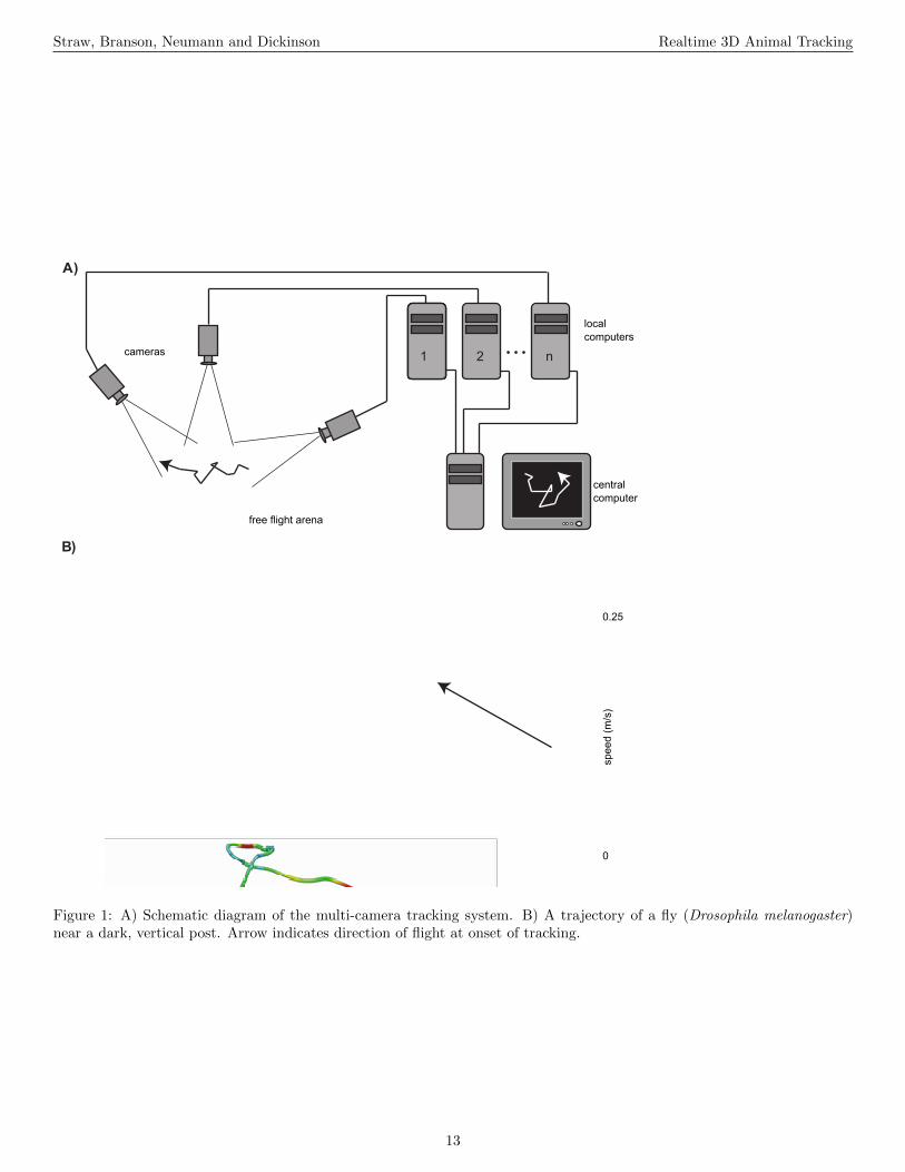
Figure 2: A) Flowchart of operations. B) Schematic illustration of a 2D camera view showing the raw images (brown),feature extraction (blue), state estimation (black), and data association (red). C) 3D reconstruction using the ExtendedKalman filter uses prior state estimates (open circle) and observations (blue lines) to construct a posterior state estimate(closed circle) and covariance ellipsoid (dotted ellipse).

14


0 5 10 15 20 25 30 35time (s)

0

500

1000

1500

2000

angu

lar

velo

city

(de

g/s)

0 50 100 150 200 250horizontal distance (mm)

90

0

90

180

270

appr

oach

ang

le (

deg)

C)

A) B)

50 mm

50 m

m

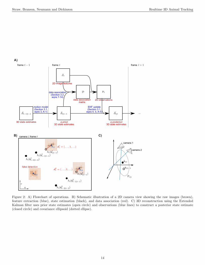
Figure 3: A) Top view of the fly trajectory in Figure 1B, showing several close approaches to and movements away from adark post placed in the center of the arena. The arrow indicates initial flight direction. Two sequences are highlighted incolor. The inset shows the coordinate system. B) The time-course of attraction and repulsion to the post is characterizedby flight directly towards the post until only a small distance remains, at which point the fly turns rapidly and flies away.Approach angle ψ is quantified as the difference between the direction of flight and bearing to the post, both measured inthe horizontal plane. The arrow indicates the initial approach for the selected sequences. C) Angular velocity (measuredtangent to the 3D flight trajectory) indicates that relatively straight flight is punctuated by saccades (brief, rapid turns).

0 msec 25 msec 50 msec 75 msec 100 msec

cam 1

cam 2

Figure 4: Raw images, 2D data extracted from the images, and overlaid computed 3D position and body orientation of ahummingbird (Calypte anna). In these images, a blue circle is drawn centered on the 2D image coordinates (u, v). The blueline segment is drawn through the detected body axis (θ in Section 3.2) when eccentricity (ε) of the detected object exceedsa threshold. The orange circle is drawn centered on the 3D estimate of position (x, y, z) reprojected through the cameracalibration matrix P, and the orange line segment is drawn in the direction of the 3D body orientation vector.

15


950

1000

y (m

m)

150 200 250 300 350

x (mm)

70

120

z (m

m)

A)

B)

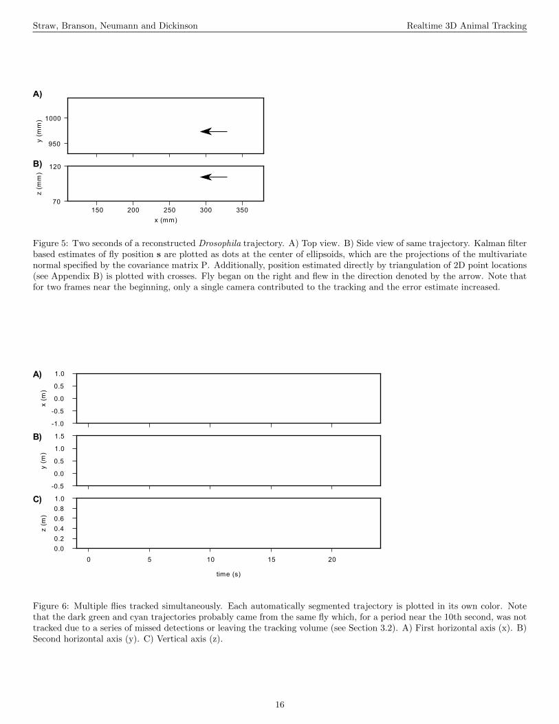
Figure 5: Two seconds of a reconstructed Drosophila trajectory. A) Top view. B) Side view of same trajectory. Kalman filterbased estimates of fly position s are plotted as dots at the center of ellipsoids, which are the projections of the multivariatenormal specified by the covariance matrix P. Additionally, position estimated directly by triangulation of 2D point locations(see Appendix B) is plotted with crosses. Fly began on the right and flew in the direction denoted by the arrow. Note thatfor two frames near the beginning, only a single camera contributed to the tracking and the error estimate increased.

-1.0

-0.5

0.0

0.5

1.0

x (m

)

-0.5

0.0

0.5

1.0

1.5

y (m

)

0 5 10 15 20

time (s)

0.0

0.2

0.4

0.6

0.8

1.0

z (m

)

A)

B)

C)

Figure 6: Multiple flies tracked simultaneously. Each automatically segmented trajectory is plotted in its own color. Notethat the dark green and cyan trajectories probably came from the same fly which, for a period near the 10th second, was nottracked due to a series of missed detections or leaving the tracking volume (see Section 3.2). A) First horizontal axis (x). B)Second horizontal axis (y). C) Vertical axis (z).

16


0 10 20 30 40 50 60 70 80latency (msec)

0

50000

100000

150000

200000

n oc

cura

nces

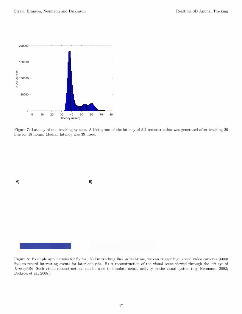
Figure 7: Latency of one tracking system. A histogram of the latency of 3D reconstruction was generated after tracking 20flies for 18 hours. Median latency was 39 msec.

B)A)

Figure 8: Example applications for flydra. A) By tracking flies in real-time, we can trigger high speed video cameras (6000fps) to record interesting events for later analysis. B) A reconstruction of the visual scene viewed through the left eye ofDrosophila. Such visual reconstructions can be used to simulate neural activity in the visual system (e.g. Neumann, 2002;Dickson et al., 2008).

17


cont rast 0.010.21± 0.11 m / s

cont rast 0.030.20± 0.11 m / s

freq

uenc

y

cont rast 0.060.17± 0.09 m / s

cont rast 0.160.15± 0.07 m / s

cont rast 0.400.15± 0.08 m / s

0.0 0.1 0.2 0.3 0.4 0.5 0.6horizontal speed (m/s)

cont rast 1.000.14± 0.07 m / s

Figure 9: Drosophila melanogaster maintain a lower flight speed with lower variability as visual contrast is increased. Meanand standard deviation of flight speeds are shown in text, and each histogram is normalized to have equal area. Ambientillumination reflected from one surface after being scattered from other illuminated surfaces slightly reduced contrast fromthe nominal values shown here.

18

Documents

Multi-camera Realtime 3D Tracking of Multiple … Realtime 3D Tracking of Multiple Flying Animals Andrew D. Straw, Kristin Branson, Titus R. Neumann & Michael H. Dickinson California