Embed Size (px)
Citation preview

1
Realtime Water Simulation on GPU
Nuttapong ChentanezNVIDIA Research
2

Overview• Approaches to realtime water simulation
• Hybrid shallow water solver + particles
• Hybrid 3D tall cell water solver + particles
• Future
3
3

Realtime Water Simulation
4
“2D” “3D”
4
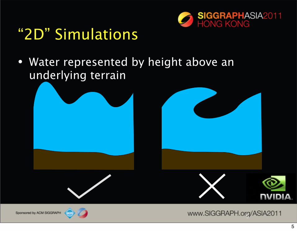
“2D” Simulations
• Water represented by height above an underlying terrain
5
5
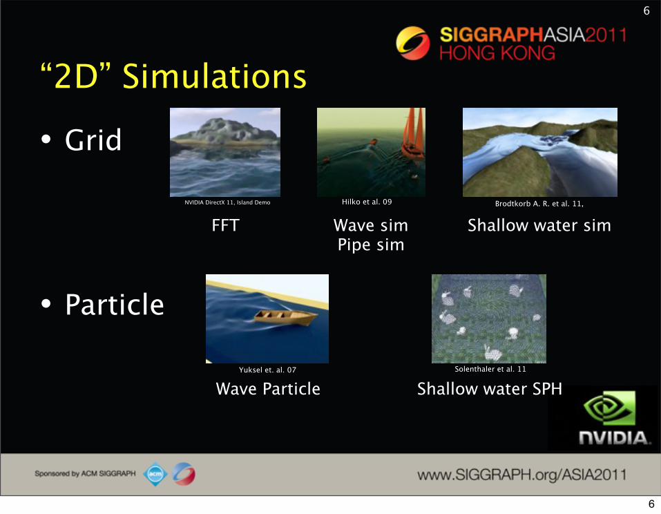
• Grid
• Particle
“2D” Simulations
6
Wave simPipe sim
FFT Shallow water sim
Wave Particle Shallow water SPH
NVIDIA DirectX 11, Island Demo
Solenthaler et al. 11Yuksel et. al. 07
Brodtkorb A. R. et al. 11, Hilko et al. 09
6
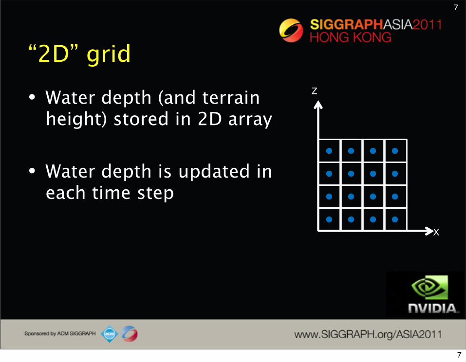
“2D” grid
• Water depth (and terrain height) stored in 2D array
• Water depth is updated in each time step
7
X
Z
7

FFT
• Fast Fourier Transform (FFT)• Represent waves as sum of sinusoids• Wave length, speed, amplitude from
statistical models• Update height and derivatives in
frequency domain• Use iFFT to transform back to spatial
domain for rendering
8
8

FFT
9
NVIDIA DirectX 11, Island Demo
9
FFT
• Pros• Fast• Great results for ocean wave, open water
• Cons• No interaction with objects• No boundary
10
10

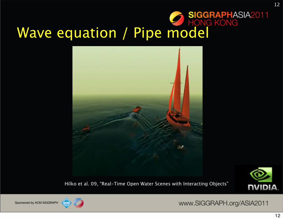
Wave equation / Pipe model
• Wave equation• Assumptions: Water surface is a height field,
velocity constant vertically, water is shallow, pressure gradient is vertical, ignore non-linear terms• Discretize temporally and spatially • Result in water height stored in 2D array +
update rules
11
11
Wave equation / Pipe model
12
Hilko et al. 09, “Real-Time Open Water Scenes with Interacting Objects”
12

Wave equation / Pipe model
• Pipe model• Water heights stored in 2D array• Neighbors are connected by pipe• Flow rate in pipes updated by heights• Heights changed by flow rate
13
13

Wave equation / Pipe model
14
Stava et al. 08, “Interactive Terrain Modeling Using Hydraulic Erosion”
14

Wave equation / Pipe model
• Pros• Still fast• Interaction with objects• Boundary
• Cons• No vortices• No large flow• Not unconditionally stable
15
15

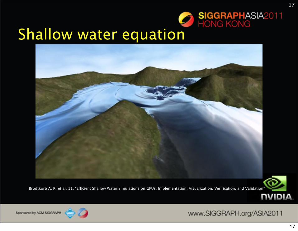
Shallow water equation• Assumptions: Water surface is a height field,
velocity is constant vertically, water is shallow, pressure gradient is vertical, with non-linear term
• Discretize temporally and spatially • Result in water height + velocity stored in 2D
array + update rules
16
16
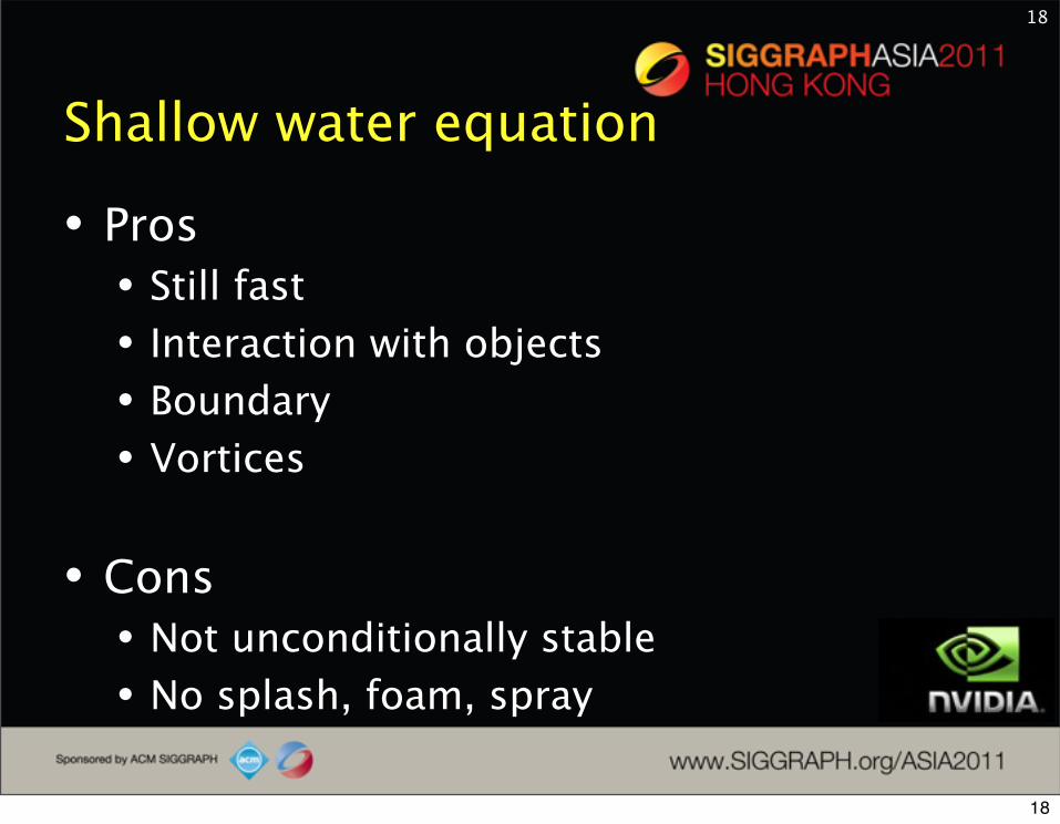
Shallow water equation
17
Brodtkorb A. R. et al. 11, “Efficient Shallow Water Simulations on GPUs: Implementation, Visualization, Verification, and Validation”
17
Shallow water equation
• Pros• Still fast• Interaction with objects• Boundary• Vortices
• Cons• Not unconditionally stable• No splash, foam, spray
18
18

Wave Particles
19
Yuksel et. al. 07, “Wave Particles”
• Particle based wave simulation• Each particle stores a waveform • Particles form wave front
• Either bounce off or leave domain boundary
19

Wave Particles
20
Yuksel et. al. 07, “Wave Particles”
20

Wave Particles
• Pros• Interaction with objects• Open boundary is easy• Unconditionally stable
• Cons• Still require grid for rendering• No vortices• No large flow
21
21

SPH Shallow Water Simulation
22
• Use Smoothed Particles Hydrodynamics (SPH) to solve shallow water equation
• Particles store mass and velocity• Kernels are centered around particles
• Volume computed by summing kernel values• Density = Mass / Volume interpreted as height
SPHERIC - SPH European Research Interest Community
22

SPH Shallow Water Simulation
23
Solenthaler et al. 11, “SPH Based Shallow Water Simulation”
23

SPH Shallow Water Simulation
• Pros• Interaction with objects• Open boundary is easy• Vortices and Flow
• Cons• Still require grid for rendering• Not unconditionally stable• Still no 3D effect!
24
24
25
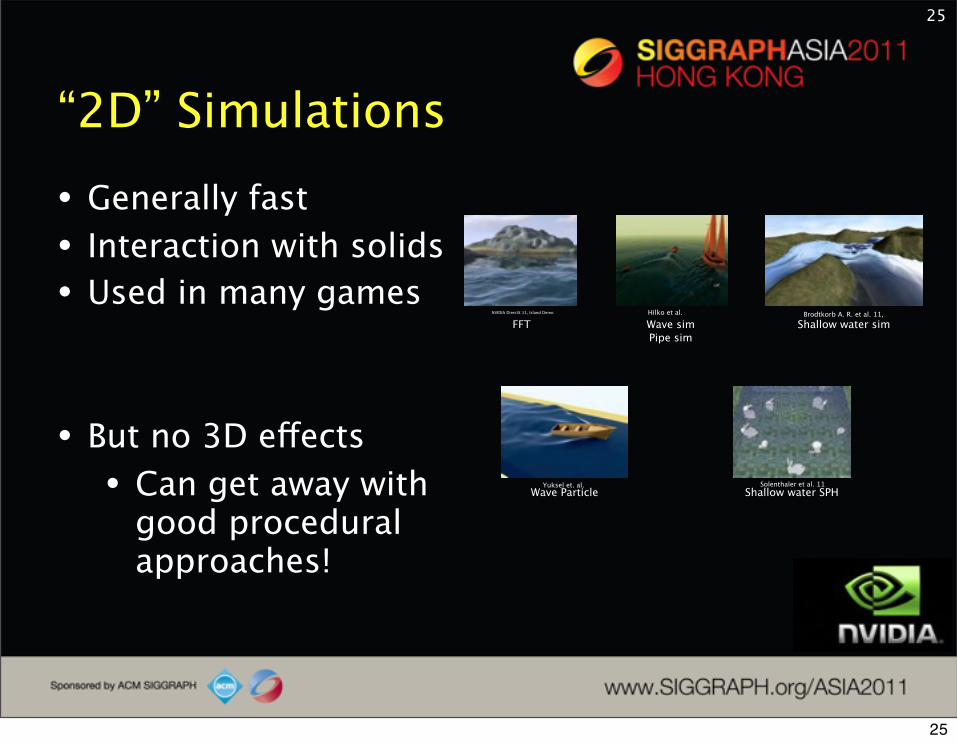
“2D” Simulations
Wave simPipe sim
FFT Shallow water sim
Wave Particle Shallow water SPH
NVIDIA DirectX 11, Island Demo
Solenthaler et al. 11Yuksel et. al.
Brodtkorb A. R. et al. 11, Hilko et al.
• Generally fast• Interaction with solids• Used in many games
• But no 3D effects• Can get away with
good procedural approaches!
25
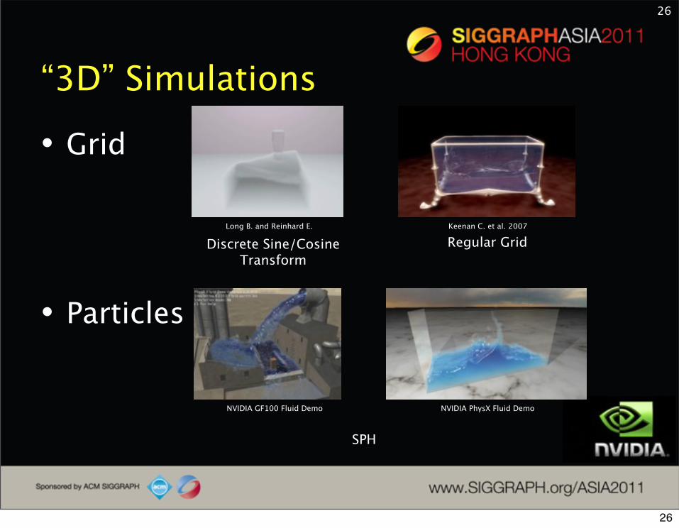
• Grid
• Particles
“3D” Simulations
26
Regular GridDiscrete Sine/Cosine Transform
SPH
Long B. and Reinhard E. Keenan C. et al. 2007
NVIDIA PhysX Fluid DemoNVIDIA GF100 Fluid Demo
26

3D grid
• Water states stored in 3D array• Velocity• Distance to surface• Density• etc.
• States are updated in each time step
27
27
Discrete Sine/Cosine Transform
28
• Use cosine and sine transform• Instead of FFT• To be able to enforce boundary condition
• Do physics in frequency domain
• Transform back to spatial domain
28

Discrete Sine/Cosine Transform
29
Long B. and Reinhard E. 09 ,”Real-Time Fluid Simulation Using Sine/Cosine Transforms”
29
Discrete Sine/Cosine Transform
• Pros• Relatively fast• Unconditionally stable
• Cons• No interaction with object• Box shape domain• No small scale details for coarse grid
30
30

Regular grid
31
• Commonly used in offline production simulation• Store water states in dense 3D grid• Solve fluid dynamics PDE by discretizing spatially
and temporally • States in the next time step determined by state
in the current time step and external forces• “Brute Force”
31
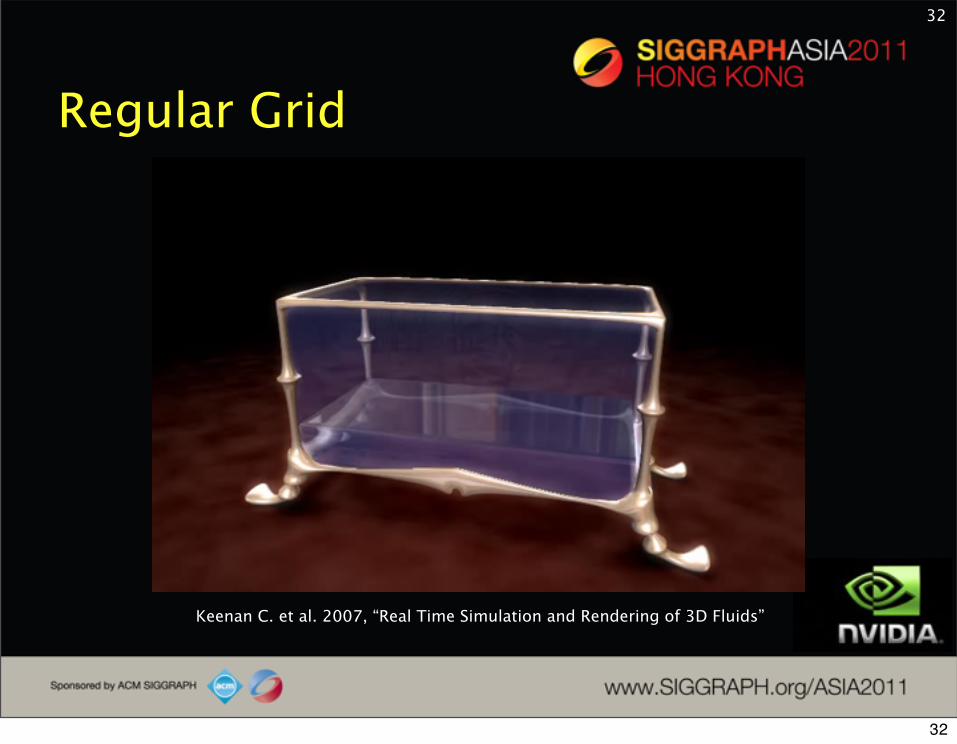
Regular Grid
32
Keenan C. et al. 2007, “Real Time Simulation and Rendering of 3D Fluids”
32
Regular Grid
• Pros• Good result• Unconditionally stable
• Cons• Box shape domain• Very computationally intensive• Mass loss• No small scale details for coarse grid
33
33
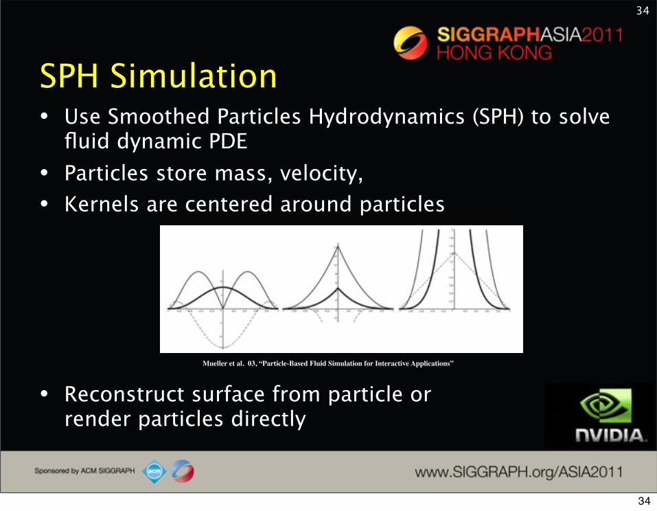
• Use Smoothed Particles Hydrodynamics (SPH) to solve fluid dynamic PDE
• Particles store mass, velocity,• Kernels are centered around particles
• Reconstruct surface from particle or render particles directly
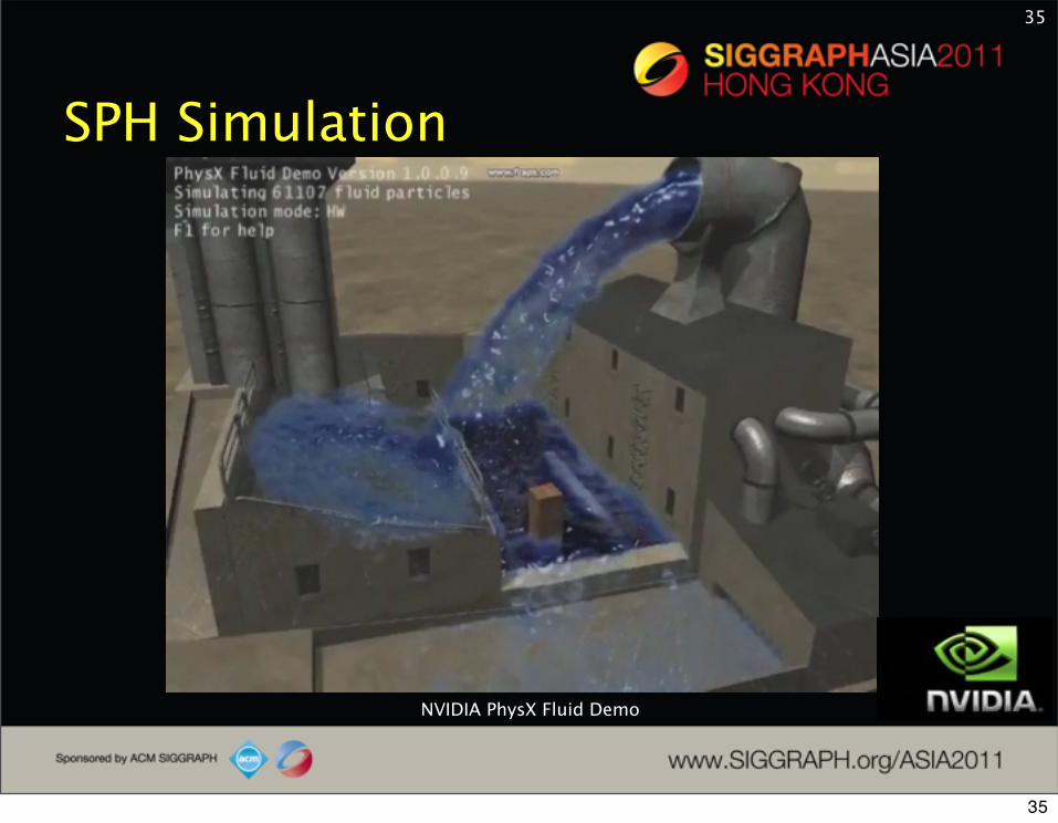
SPH Simulation
34
Mueller et al. 03, “Particle-Based Fluid Simulation for Interactive Applications”
34
SPH Simulation
35
NVIDIA PhysX Fluid Demo
35
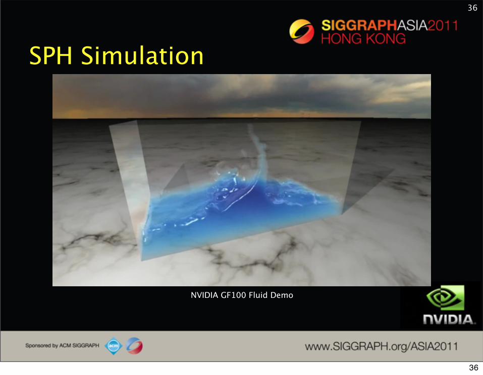
SPH Simulation
36
NVIDIA GF100 Fluid Demo
36
SPH Simulation
• Pros• Arbitrary domain• Interaction with object• No mass loss
• Cons• Noisy surface• Not unconditionally stable
37
37

38
“3D” Simulations• At high resolution,
produce great results• Widely used in
movie industry
• Can’t afford to do large scene with small scale details
26
Regular GridDiscrete Sine/Cosine Transform
SPH
Long B. Keenan C.
NVIDIA PhysX Fluid NVIDIA GF100 Fluid
38

Overview• Approaches to realtime water simulation
• Hybrid shallow water solver + particles
• Hybrid 3D tall cell water solver + particles
• Future
39
39
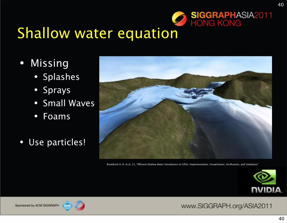
Shallow water equation
40
Brodtkorb A. R. et al. 11, “Efficient Shallow Water Simulations on GPUs: Implementation, Visualization, Verification, and Validation”
• Missing• Splashes• Sprays• Small Waves• Foams
• Use particles!
40
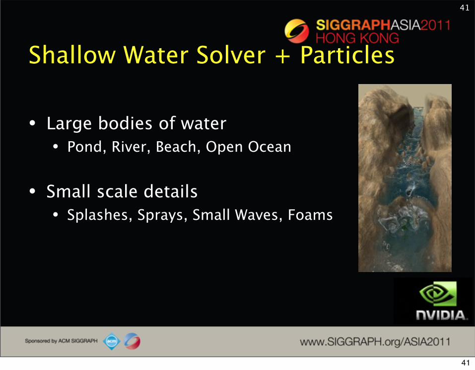
Shallow Water Solver + Particles
• Large bodies of water• Pond, River, Beach, Open Ocean
• Small scale details• Splashes, Sprays, Small Waves, Foams
41
41

Shallow Water Solver + Particles
42
Chentanez N. and Mueller M. 2010, “Real-time Simulation of Large Bodies of Water with Small Scale Details”
42
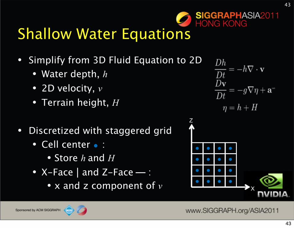
Shallow Water Equations• Simplify from 3D Fluid Equation to 2D• Water depth, h• 2D velocity, v• Terrain height, H
• Discretized with staggered grid• Cell center :• Store h and H
• X-Face and Z-Face :• x and z component of v
43
X
Z
43

Particles Simulation
• Particles sources• Waterfalls• Terrain height discontinuity,
create spray and splash
• Breaking waves• When wave about to overturn,
create spray and splash
44
44

Particles Simulation
• Particles sources• Falling splash• Create spray and foam
• Solid interaction• Create spray and splash
45
45

Waterfall• We treat a face as a waterfall face if• Terrain height change is greater than a
threshold and• Water height in the lower cell has not yet
reached the terrain height in the higher cell
46
46

Waterfall• Particles generation
• Sample uniformly within red dotted box• Total mass should be the same as mass flow
across the face• Velocity found by interpolation• Jitter initial position and velocity
47
47

Waterfall
48
48
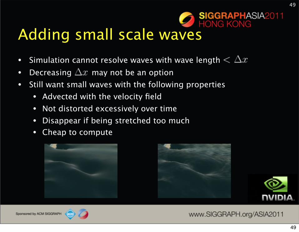
Adding small scale waves• Simulation cannot resolve waves with wave length• Decreasing may not be an option• Still want small waves with the following properties
• Advected with the velocity field• Not distorted excessively over time• Disappear if being stretched too much• Cheap to compute
49
49
Adding small scale waves
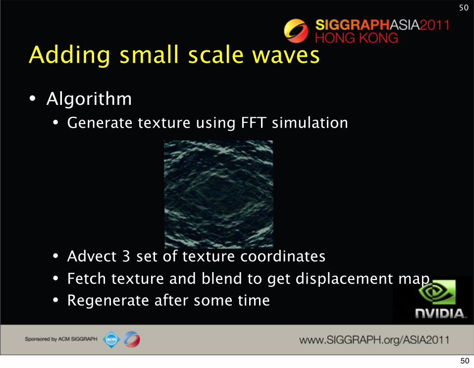
• Algorithm • Generate texture using FFT simulation
• Advect 3 set of texture coordinates• Fetch texture and blend to get displacement map• Regenerate after some time
50
50

Adding small scale waves• So far, waves will never disappear• Wave persist even when being stretched a lot• Can have lava-like look• Need to suppress in region with too much stretch
51
Without suppressant With suppressant
51
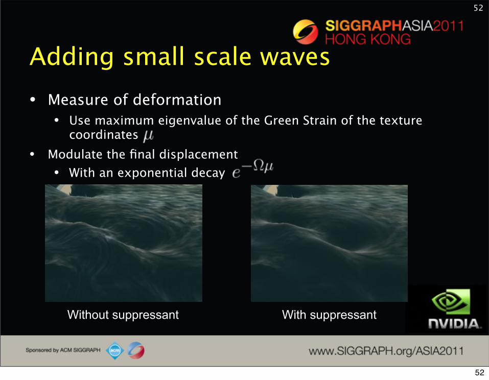
Adding small scale waves• Measure of deformation
• Use maximum eigenvalue of the Green Strain of the texture coordinates
• Modulate the final displacement• With an exponential decay
52
Without suppressant With suppressant
52

Adding small scale waves
53
53

More results
54
54

More results
55
55

Overview• Approaches to realtime water simulation
• Hybrid shallow water solver + particles
• Hybrid 3D tall cell water solver + particles
• Future
56
56

Grid based 3D water simulation• Small domain
• Computation increase with volume of water
• Also want small scale details• Splash• Foam• Spray
57
Keenan C. et al. 2007, “Real Time Simulation and Rendering of 3D Fluids”
57
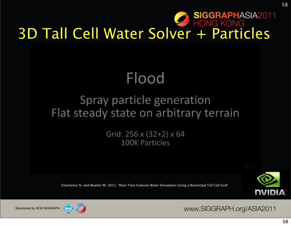
3D Tall Cell Water Solver + Particles
58
Chentanez N. and Mueller M. 2011, “Real-Time Eulerian Water Simulation Using a Restricted Tall Cell Grid”
58

3D Tall Cell Water Solver + Particles
59
59
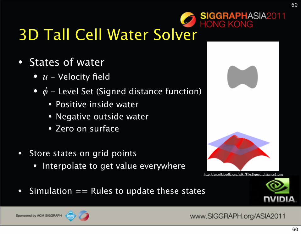
3D Tall Cell Water Solver• States of water • u - Velocity field
• ϕ - Level Set (Signed distance function)• Positive inside water• Negative outside water• Zero on surface
• Store states on grid points• Interpolate to get value everywhere
• Simulation == Rules to update these states
60
http://en.wikipedia.org/wiki/File:Signed_distance2.png
60
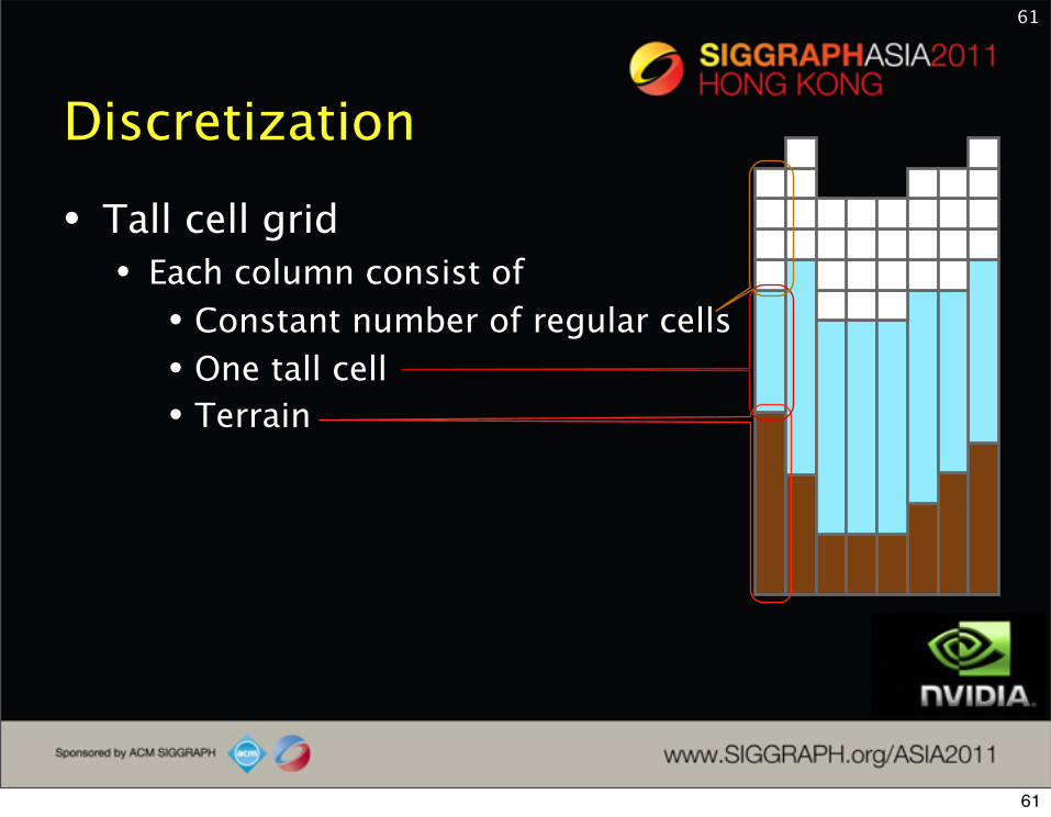
Discretization
• Tall cell grid• Each column consist of• Constant number of regular cells• One tall cell• Terrain
61
61
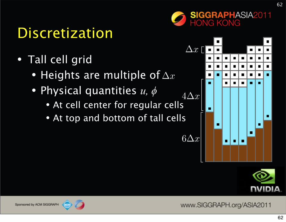
Discretization
• Tall cell grid• Heights are multiple of• Physical quantities u, ϕ• At cell center for regular cells• At top and bottom of tall cells
62
∆x
4∆x
6∆x
∆x
62

Discretization• Tall cell grid• Quantity at world position
denoted by• Hide tall cell structure of the grid
63
Direct lookup
Linear interpolation
q (x∆x, y∆x, z∆x)
“Air value”
“Terrain value”
q(x, y, z)
63

Time integration
64
Extrapolate u to air
64
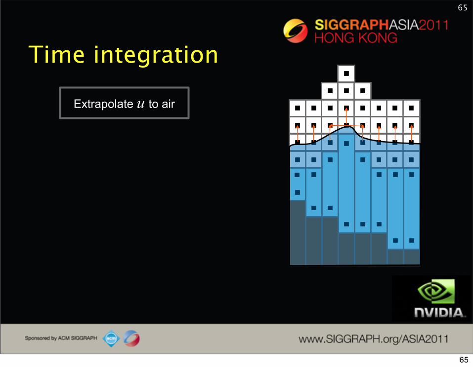
Time integration
65
Extrapolate u to air
65

Time integration
66
Extrapolate u to air
66

Time integration
67
Extrapolate u to air
67

Time integration
68
Because ϕ will no longer be a signed distance function, as we update the states
Extrapolate u to air
Make ϕ a signed distance function
68

Time integration
69
Extrapolate u to air
Make ϕ a signed distance function
69

Time integration
70
Extrapolate u to air
Make ϕ a signed distance function
70

Time integration
71
Extrapolate u to air
Make ϕ a signed distance function
71

Time integration
72
Extrapolate u to air
Make ϕ a signed distance function
Move u and ϕ along velocity field u
72

Time integration
73
Extrapolate u to air
Make ϕ a signed distance function
Move u and ϕ along velocity field u
73
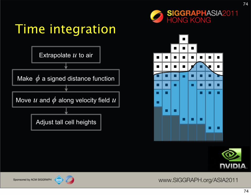
Time integration
74
Extrapolate u to air
Make ϕ a signed distance function
Move u and ϕ along velocity field u
Adjust tall cell heights
74

Time integration
75
Extrapolate u to air
Make ϕ a signed distance function
Move u and ϕ along velocity field u
Adjust tall cell heights
75

Time integration
76
Extrapolate u to air
Make ϕ a signed distance function
Move u and ϕ along velocity field u
Adjust tall cell heights
Make u divergence freeThe most difficult and time consuming step
76

Particles• Spray
• Seed particles inside grid cells whose ϕ are positive but small (near water surface)
• Move them along velocity field u• After we update ϕ, for each particle
• Check if ϕ at the current location is negative (outside water)• If so, generate spray particles• otherwise, ignore
• Move ballistically
• Foam• Generate when spray particle falls into water• Move with u, projected to water surface
77
77

More result
78
Chentanez N. and Mueller M. 2011, “Real-Time Eulerian Water Simulation Using a Restricted Tall Cell Grid”
78

Future
• Hybrid 3D + 2D + Particles + Procedural?• 3D + Particles near camera• 2D + Particles further away• 2D even further• Procedural far from camera
79
79
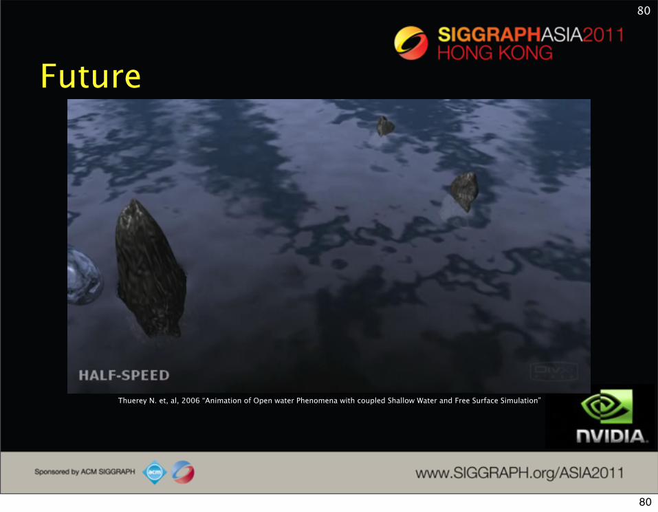
Future
80
Thuerey N. et, al, 2006 “Animation of Open water Phenomena with coupled Shallow Water and Free Surface Simulation”
80

Future
81
Thuerey N. et, al, 2006 “Animation of Open water Phenomena with coupled Shallow Water and Free Surface Simulation”
81
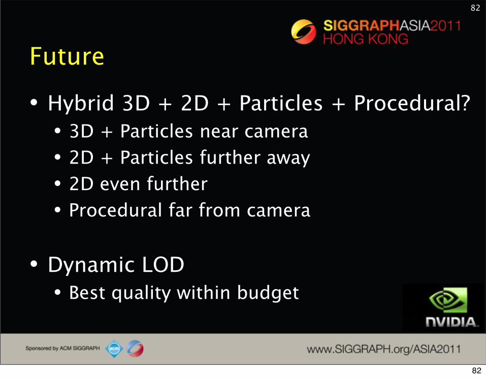
Future
• Hybrid 3D + 2D + Particles + Procedural?• 3D + Particles near camera• 2D + Particles further away• 2D even further• Procedural far from camera
• Dynamic LOD • Best quality within budget
82
82

Q&A
83
Thank you very much!
83

References• Tessendof SIGGRAPH Course 99, “Simulating Ocean Wave”
• Enright et al. SIGGRAPH 02, “Animation and Rendering of Complex Water Surfaces”
• Mueller et al. SCA 03, “Particle-Based Fluid Simulation for Interactive Applications”
• Thuerey N. et, al, SCA 06 “Animation of Open water Phenomena with coupled Shallow Water and Free Surface Simulation”
• Keenan C. et al. GPU Gems III 07, “Real Time Simulation and Rendering of 3D Fluids”
• Yuksel et. al. SIGGRAPH 07, “Wave Particles”
• Stava et al. SCA 08, “Interactive Terrain Modeling Using Hydraulic Erosion”
• Hilko et al. Eurographics workshop on natural phenomena 09, “Real-Time Open Water Scenes with Interacting Objects”
• Long B. and Reinhard E. I3D 09 ,”Real-Time Fluid Simulation Using Sine/Cosine Transforms”
• Chentanez N. and Mueller M. SCA 10, “Real-time Simulation of Large Bodies of Water with Small Scale Details”
• Brodtkorb A. R. et al. Computer & Fluid 11, “Efficient Shallow Water Simulations on GPUs: Implementation, Visualization, Verification, and Validation”
• Chentanez N. and Mueller M. SIGGRAPH 11, “Real-Time Eulerian Water Simulation Using a Restricted Tall Cell Grid
84
84
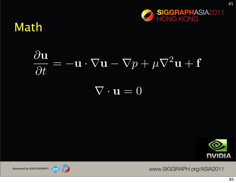
∇ · u = 0
Math
85
∂u
∂t= −u ·∇u−∇p+ µ∇2u+ f
85
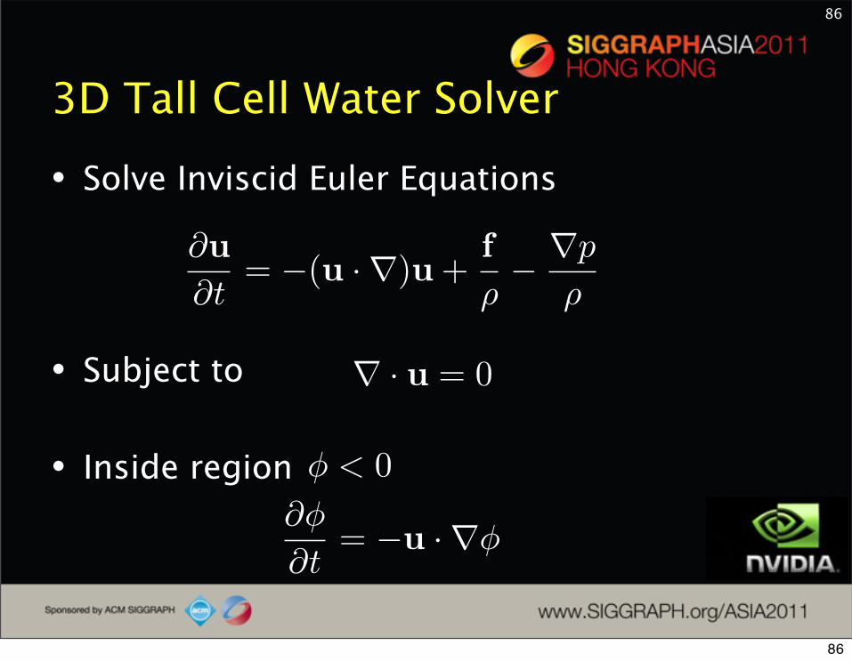
3D Tall Cell Water Solver
• Solve Inviscid Euler Equations
• Subject to
• Inside region
86
∂u
∂t= −(u ·∇)u+
f
ρ− ∇p
ρ
∇ · u = 0
φ < 0
∂φ
∂t= −u ·∇φ
86

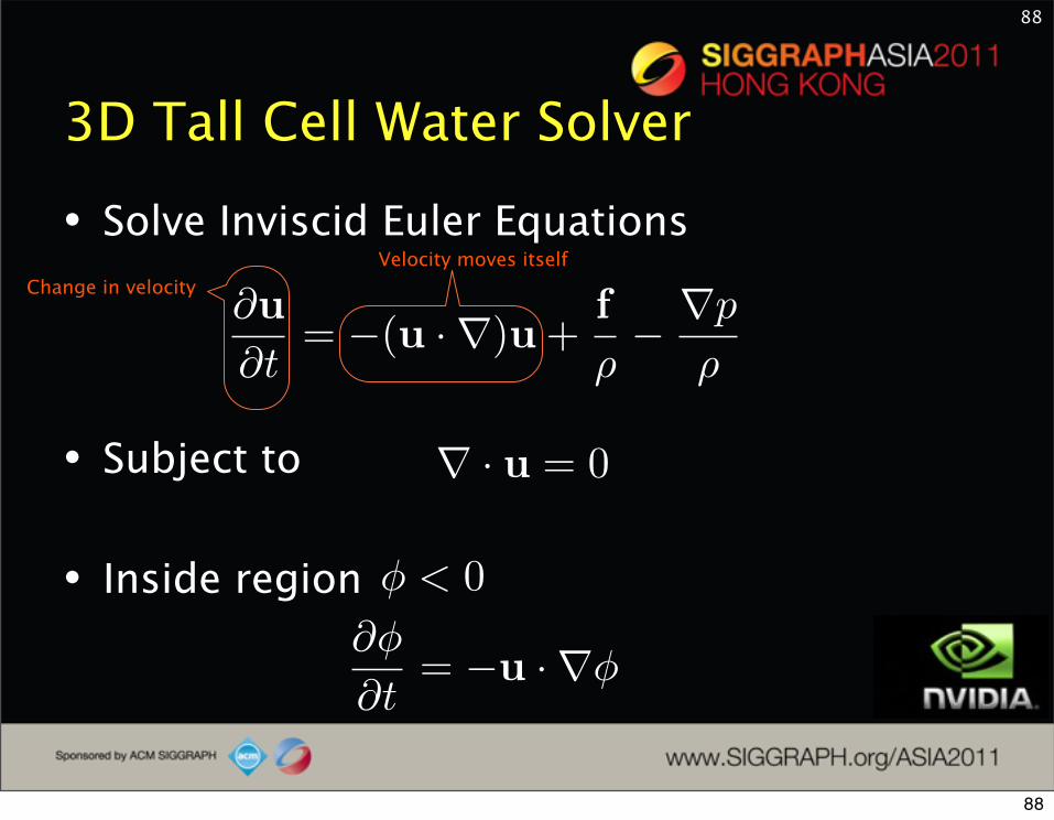
3D Tall Cell Water Solver
• Solve Inviscid Euler Equations
• Subject to
• Inside region
87
∂u
∂t= −(u ·∇)u+
f
ρ− ∇p
ρ
∇ · u = 0
φ < 0
∂φ
∂t= −u ·∇φ
Change in velocity
87
3D Tall Cell Water Solver
• Solve Inviscid Euler Equations
• Subject to
• Inside region
88
∂u
∂t= −(u ·∇)u+
f
ρ− ∇p
ρ
∇ · u = 0
φ < 0
∂φ
∂t= −u ·∇φ
Change in velocityVelocity moves itself
88
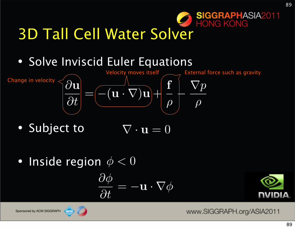
3D Tall Cell Water Solver
• Solve Inviscid Euler Equations
• Subject to
• Inside region
89
∂u
∂t= −(u ·∇)u+
f
ρ− ∇p
ρ
∇ · u = 0
φ < 0
∂φ
∂t= −u ·∇φ
Change in velocityVelocity moves itself External force such as gravity
89

3D Tall Cell Water Solver
• Solve Inviscid Euler Equations
• Subject to
• Inside region
90
∂u
∂t= −(u ·∇)u+
f
ρ− ∇p
ρ
∇ · u = 0
φ < 0
∂φ
∂t= −u ·∇φ
Change in velocityVelocity moves itself External force such as gravity
Pressure gradient
90

3D Tall Cell Water Solver
• Solve Inviscid Euler Equations
• Subject to
• Inside region
91
∂u
∂t= −(u ·∇)u+
f
ρ− ∇p
ρ
∇ · u = 0
φ < 0
∂φ
∂t= −u ·∇φ
Change in velocityVelocity moves itself External force such as gravity
Pressure gradient
Incompressibility- What come in must go out
91

3D Tall Cell Water Solver
• Solve Inviscid Euler Equations
• Subject to
• Inside region
92
∂u
∂t= −(u ·∇)u+
f
ρ− ∇p
ρ
∇ · u = 0
φ < 0
∂φ
∂t= −u ·∇φ
Change in velocityVelocity moves itself External force such as gravity
Pressure gradient
Incompressibility- What come in must go out
Implicit function that represent water body
92

3D Tall Cell Water Solver
• Solve Inviscid Euler Equations
• Subject to
• Inside region
93
∂u
∂t= −(u ·∇)u+
f
ρ− ∇p
ρ
∇ · u = 0
φ < 0
∂φ
∂t= −u ·∇φ
Change in velocityVelocity moves itself External force such as gravity
Pressure gradient
Incompressibility- What come in must go out
Implicit function that represent water body
Implicit function movedby water velocity
93