MT and ST PASA

MT and ST PASA –Modelling Concepts and ScenariosWRIG – 24 June 2021

Agenda

2

1. Recap Section 3.16 of the WEM Rules

2. Understanding Key Componentsa) ST and MT PASA Market Model Concept

b) Inputs and Pre-processing

c) ST and MT Scenarios Modelling

d) Outputs & Post -Processing

3. Next Steps

Section 3.16A of the WEM Rules – Projected Assessment of System Adequacy (PASA)

• AEMO will be required to conduct periodic PASA assessments and publish a rolling MT PASA and ST PASA as set out in clause 3.16.1• At least each week of the 36 month period from the starting date of the assessment (MT PASA)

• At least each day of the seven day period from the starting date of the assessment (ST PASA)

• Clause 3.16.2 set out the new PASA objective linking it to Power System Security and Power System Reliability framework.

• Clause 3.16.3 set out the obligation on Rule Participants to provide the information for AEMO to conduct and prepare MT PASA and ST PASA. Details of the information required will be set out in the WEM Procedure.

• Clause 3.16.7 deals with forecasting, specifically the 36-month forecast as the week ahead forecast is covered in the SCED rules under 7.3 (Forecast Operational Demand).

• Clause 3.16.8 sets out the core requirements of the MT and ST PASA report which are linked to the objectives set out in clause 3.16.2.

• Clause 3.16.9 enables AEMO to issue an updated MT PASA or ST PASA where there has been a material change.

• Clause 3.16.10 provides head of power for AEMO to develop WEM Procedure which contains the details in respect of the PASA framework.

ST PASA Market Model

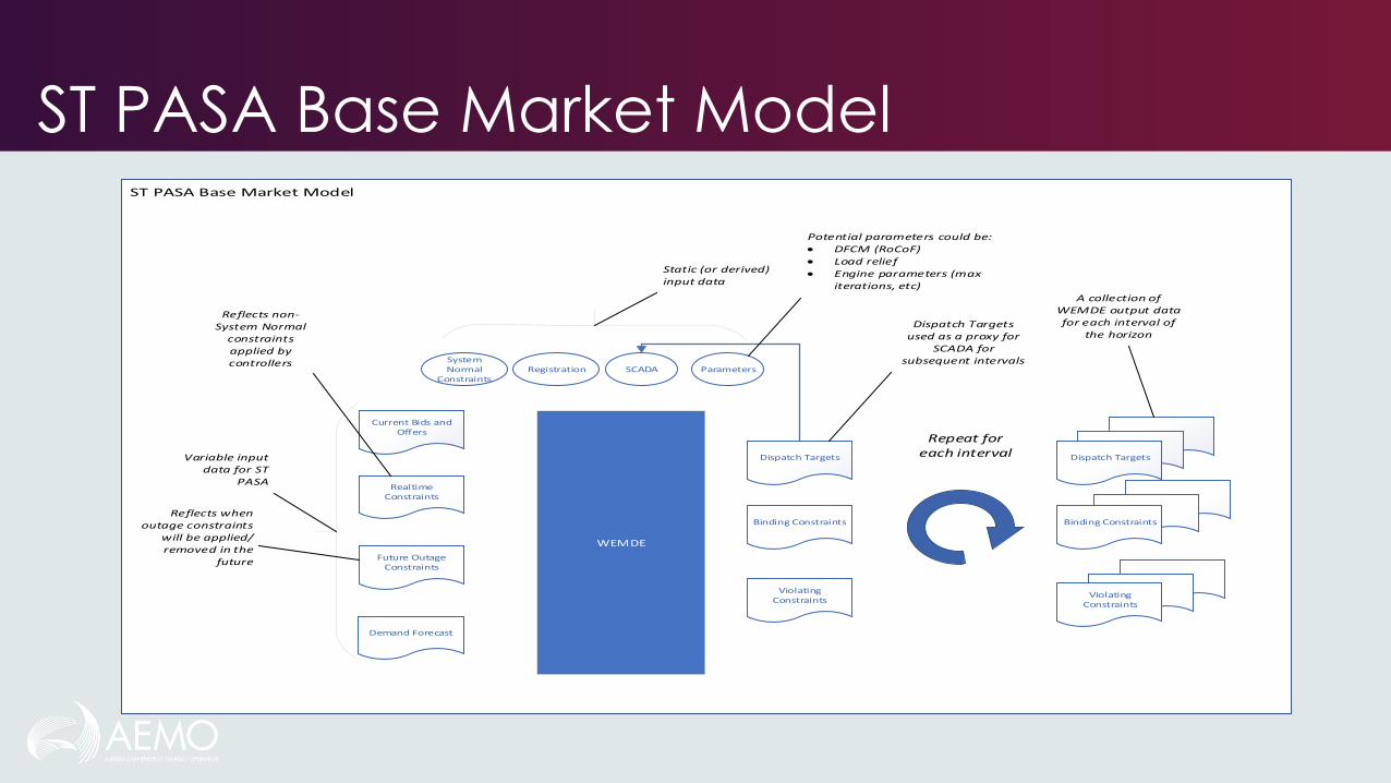
ST PASA Base Market Model

Current Bids and Offers

WEMDE

Realtime Constraints

Future Outage Constraints

Demand Forecast

Dispatch Targets

Binding Constraints

Violating Constraints

Dispatch Targets

Binding Constraints


Repeat for each interval

SCADA ParametersRegistrationSystem Normal

Constraints

Variable input data for ST

PASA

Static (or derived) input data

Dispatch Targets used as a proxy for

SCADA for subsequent intervals

A collection of WEMDE output data for each interval of

the horizon

Reflects non-System Normal

constraints applied by controllers

Reflects when outage constraints

will be applied/removed in the

future

Potential parameters could be:• DFCM (RoCoF)• Load relief • Engine parameters (max

iterations, etc)

ST PASA Scenario's Modelling

Overview ST PASA Conceptual Diagram


Current Realtime Constraints

Known Future Outage Constraints

Expected Demand Forecast

Publish the following:

• Full data report of all intervals for each scenario

Identify the following:

• Not enough online capacity to meet demand (violating energy constraint)

• Shortages of ESS (violating ESS constraints)

• Other security issues (other violating constraints)

• Occurrence of network constraints binding

• Occurrence of DSP dispatch

And determine likelihood based on:

• Number of occurrences• Scenario combinations that

occurrences appear in

WEMDE

Varied Bids and Offers

Bids and Offers

Varied Realtime Constraints

Varied Outage Constraints


Demand Forecast

Constraints

Outages

Demand


Dispatch Targets

Binding Constraints


Dispatch Targets

Binding Constraints


Dispatch Targets

Binding Constraints


Repeat for each combination of input scenarios

• Identify and issue Low Reserve Notifications

• Identify and manage any dispatch interventions



Constraints

Different NSG/SSG Forecast Quantities

Unplanned Outages

Variations on in/out of service quantities

Changes to outage start/completion times

Different demand scenarios

Combinations of input data to form

input scenario s

Different variations of input data (see below for examples)

A collection of output data for

each interval in the horizon, from each

of the different scenario s

Run output processing on the data to identify risks

Highlight type of LRC and likelihood of occurrence

Variations on DSP available quantities


Inputs and Pre-processing


Current Realtime Constraints

Known Future Outage Constraints



Varied Realtime Constraints

Varied Outage Constraints


Demand Forecast


Different NSG/SSG Forecast Quantities

Unplanned Outages

Variations on in/out of service quantities



Variations on DSP available quantities

ST PASA Input VariationsInput variations considerations

Intermittent (NSG/SSG) variations• I1 - Base (per offers)• I2 - Base + statistical error margin (e.g. per Facility, per time of year/

time of day)• I3 - High output (e.g. 95% capacity)• I4 - Low output (e.g. 5% capacity)• I5 - Reserve capacity levels

Availability (In/Out of Service Quantity) variations• A1 - Base (per offers)• A2 - Base + adjusting in service quantities for large/key Facilities to zero

Realtime Constraint variations• RT1 - Base (currently applied realtime constraints)• RT2 - Base + random forced outages (e.g. based on statistical outage

rates)• RT3 - Base + largest remaining contingencies

Future Outage variations• O1 - Base (current planned outage start/finish times)• O2 - Early commencement/late finish variations• O3 - Base + largest network contingency

DSP available quantity variations• DSP1 - Base (per offers)• DSP2 - Base + statistical error margin (e.g. per

DSP, per time of year/time of day)• DSP3 – low availability (5% capacity)

Demand variations• D1 - Expected demand• D2 - Expected demand + statistical error margin• D3 - Expected demand + low PV output• D4 - Expected demand + high PV output• D5 - Expected demand + highly variable PV

output• D6 - High demand• D7 - Low demand• D8 - POE10 demand

We will define valid combinations of these input variations to form the overall list of input scenario s for ST PASA

E.g.

• Base scenario (all base input data) = I1, DSP1, A1, RT1, O1, D1• High capacity risk scenario = I4, DSP3, A2, RT3, O2, D7• Medium capacity risk scenario = I2, DSP2, A1, RT3, O2, D5Etc

Scenario’s Modelling

WEMDE

Bids and Offers

Constraints

Outages

Demand


Dispatch Targets

Binding Constraints


Dispatch Targets

Binding Constraints


Dispatch Targets

Binding Constraints




Constraints

Combinations of input data to form

input scenario s

A collection of output data for

each interval in the horizon, from each

of the different scenario s


Outputs Post Processing
















ST PASA: Data Requirements

• Given shorter timeframes, most information is expected to come through offers

• Will need modelling data from participants to support estimating different output scenarios (e.g. wind turbine power curves)

• Variability estimated from historical data

• Risks based on including contingency events (e.g. loss of next largest generator, major transmission outage, loss of major ESS provider, etc)

MT PASA Market Model

MT PASA Market Model: Key Requirements

• Approximation of single node wholesale electricity market model

• Mixed integer linear programming (MILP) solver to co-optimise energy and essential system services provision for every 30-min interval in the MT PASA horizon (time-sequential)

• Handles linear constraint equations (security-constrained dispatch)

• Determines estimates of unit commitment (time-sequential over specified commitment horizon)

• Randomised generator forced outages

• Uses generator planned outage schedules

• Assesses Power System Security/Reliability risks based on different input scenarios

MT PASA Base Market Model

Market model (e.g. Plexos) based on :• co-optimised (energy & ESS), • gross pool,• single node with linear network constraints provided from external source

Market Model manages the modelling inputs such as:Unit CommitmentFacility bid creation (Economic parameters)Synthetic maintenance outages (monte carlo)Randomised forced outages (monte carlo)ESS Requirements (CR and RoCof)

Future Network Outage /ESS Constraints

Demand Forecast

Dispatch Targets

Binding Constraints

Unserved Energy

Repeat for cost variability(internal in

model)

Intermittent Forecast

Dispatch Targets

Binding Constraints

Unserved Energy

Loss FactorsFacility and

Standing DataGenerator

Planned OutagesSystem Normal

Constraints

Future generator/network

augmentation

Other Rule Participant Data

DSP Forecast Available Quantities

LOLP

Variable input data for MT PASA


A collection of output data for each interval of the horizon allowing for price sensitivity

Reflects when outage/ESS

constraints will be applied/removed

in the future

A collection of output data for each interval

of the horizon

Assumptions around known changes to the power system (e.g. new generators, network changes)

Information such as heat rates, fixed/variable O&M, fuel costs/contracts, energy constraints, unit modelling data/limits)

MT PASA Scenario’s Modelling

Overview MT PASA Conceptual Diagram












Market model (e.g. Plexos) based on :co-optimised (energy & ESS), gross pool,single node with linear network constraints provided

Market Model manages the modelling inputs such as:Unit CommitmentFacility bid creation (Economic parameters)Synthetic maintenance outages (monte carlo)Randomised forced outages (monte carlo)ESS Requirements (CR and RoCof)

Intermittent Forecasts

Outages

Demand


model)


Dispatch Targets

Binding Constraints

Unserved Energy

Dispatch Targets

Binding Constraints

Unserved Energy

Dispatch Targets

Binding Constraints

Unserved Energy

Dispatch Targets

Binding Constraints

Unserved Energy




Standing Data

Generator Planned Outages

System Normal Constraints

Future generator/

network augmentation


DSP availability

Known Future Network Outage

Constraints


Varied Network Outage Constraints

Demand Forecast


DSP Available Quantities

Other Rule Participant

Data

Future generator/


System Normal

Constraints


Loss Factors

Facility and Standing Data

Combinations of input data to form input scenario s

A collection of output data for each interval in the horizon, from each of the different

scenario s


A collection of output data for each interval of

the horizon



Assumptions around known changes to the power system (e.g. new generators, network changes)

Information such as heat rates, fixed/variable O&M, fuel costs/contracts, energy constraints, unit modelling data/limits)




Different intermittent generation forecasts

Different DSP availability assumptions


Inputs and Pre-processing

Known Future Network Outage

Constraints


Varied Network Outage Constraints

Demand Forecast


DSP Available Quantities

Other Rule Participant

Data

Future generator/


System Normal

Constraints


Loss Factors

Facility and Standing Data




Different intermittent generation forecasts

Different DSP availability assumptions


MT PASA Input Variations

Input variations considerations:

Intermittent (NSG/SSG) variations:• I1 – Statistical time of year (e.g. per Facility, per time of year/time of day)• I2 - High output (e.g. 95% capacity)• I3 - Low output (e.g. 5% capacity)• I4 - Reserve capacity levels

DSP available quantity variations:• DSP1 - Base (per offers)• DSP2 - Base + statistical error margin (e.g. per DSP, per time of year/time of

day)• DSP3 – low availability (5% capacity)

Future Outage variations:• O1 - Base (current planned outage start/finish times)• O2 - Early commencement/late finish variations• O3 - Base + largest network contingency

Demand variations:• D1 - Expected demand• D2 - High demand• D3 - Low demand• D4 - POE10 demand• D5 – POE50 demand

We will define valid combinations of these input variations to form the overall list of input scenario s for MT PASA

E.g.

• Base scenario = I1, DSP1, O1, D1• High capacity risk scenario = I3, DSP3, O3, D4• Medium capacity risk scenario = I4, DSP2, O2, D2Etc

Scenario’s Modelling

Market model (e.g. Plexos) based on :• co-optimised (energy & ESS), • gross pool,• single node with linear network constraints provided

Market Model manages the modelling inputs such as:• Unit Commitment• Facility bid creation (Economic parameters)• Synthetic maintenance outages (monte carlo)• Randomised forced outages (monte carlo)• ESS Requirements (CR and RoCof)

Intermittent Forecasts

Outages

Demand


model)


Dispatch Targets

Binding Constraints

Unserved Energy

Dispatch Targets

Binding Constraints

Unserved Energy

Dispatch Targets

Binding Constraints

Unserved Energy

Dispatch Targets

Binding Constraints

Unserved Energy


Standing Data


System Normal Constraints

Future generator/



DSP availability

Combinations of input data to form input scenario s

A collection of output data for each interval in the horizon, from each of the different

scenario s

A collection of output data for each interval of

the horizon


Assumptions around known changes to the power system (e.g. new generators, network changes)Information such as heat rates,

fixed/variable O&M, fuel costs/contracts, energy constraints, unit modelling data/limits)

Outputs Post Processing
















MT PASA: Data Requirements

• Will need modelling data from participants to support estimating output (e.g. wind turbine power curves)

• May require information from Demand Side Programmes on future demand estimates (e.g. future demand availability reductions)

• Information on future network augmentations and decommissioning

• Information on future generation connections

• Information on future generation retirements

Questions

23

Next Steps

• We will continue to build on the modelling concepts and scenarios

• Commence drafting the WEM Procedure

Documents

MT and ST PASA