Embed Size (px)
Citation preview

Outline • General principals
– Origin of the signal
– RF excitation
– Relaxation (T1, T2, …)
• Anatomical imaging
– Image contrast
– Standard acquisition methods
– Advanced acquisition methods
• Functional imaging
– BOLD effect
– Limitations of fMRI acquisitions
– Advanced methods

Outline • General principals
– Origin of the signal
– RF excitation
– Relaxation (T1, T2, …)
• Anatomical imaging
– Image contrast
– Standard acquisition methods
– Advanced acquisition methods
• Functional imaging
– BOLD effect
– Limitations of fMRI acquisitions
– Advanced methods

Origin of the signal
Rotating magnet induces an electric current in the coil Bicycle
dynamo
M0
MRI Rotating magnetization M0 induces an signal in the head coil
receive coil

Origin of the signal
M0
O
H
H
Water molecule
• MRI signal arises from water molecules surrounding brain tissue NOT from tissue itself • The higher the water concentration (proton density) the stronger the signal

Hardware
B0 B0
B0 is oriented along the main direction of the bore
The receive coil detects signal arising from the magnetization
Magnetic field B0 created by superconducting magnet
receive coil
Layout - orientation
(x,y) plane: perpendicular to receive coil Transverse plane
z direction: aligned with receive coil Longitudinal direction
z
y
x
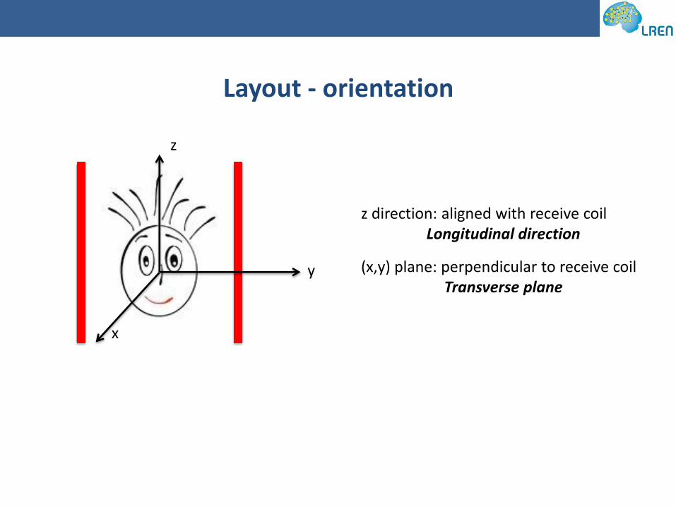
Layout - orientation
Magnetization M0 has a longitudinal component along the z-direction Magnetization M0 has a transverse component in the x-y plane
z
y
x
M0 Ml
Mt

RF excitation
M0
At rest: M0 is along the longitudinal direction
Signal cannot be detected
RF excitation
M0
After RF excitation: M0 is in the transverse plane
Signal can be detected
All MR sequences require RF excitation

Return to equilibrium
M0
RF
M0 M0
After RF excitation M0 returns to its initial state (equilibrium)
t
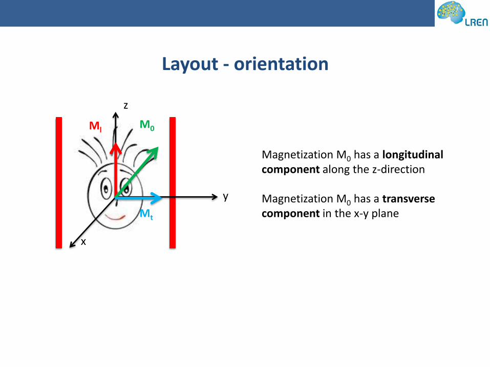
Return to equilibrium
RF
M0 Ml
Mt
Ml Ml
Equilibrium Equilibrium

t
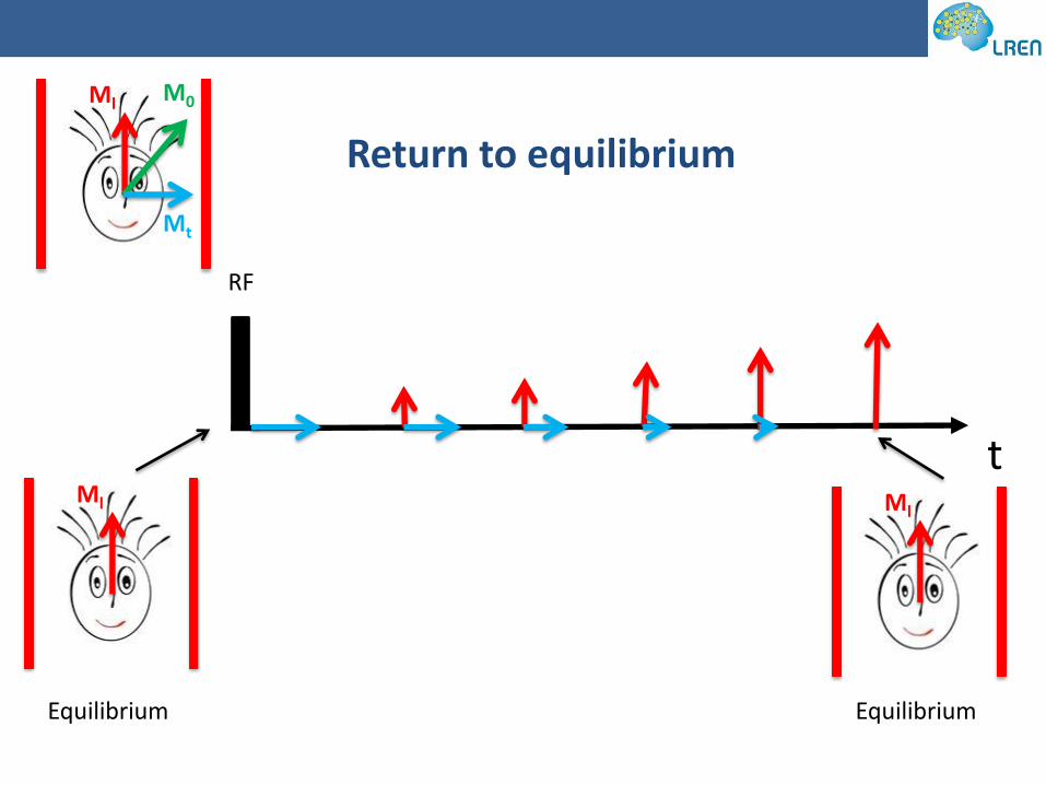
Return to equilibrium
RF
M0 Ml
Mt
T2 T1
Following RF excitation M0: - Longitudinal component of M0 increases. Recovery time T1 - Transverse component of M0 decreases. Decay time T2

Outline • General principals
– Origin of the signal
– RF excitation
– Relaxation (T1, T2, …)
• Anatomical imaging
– Image contrast
– Standard acquisition methods
– Advanced acquisition methods
• Functional imaging
– BOLD effect
– Limitations of fMRI acquisitions
– Advanced methods

Anatomical imaging requirements
• Optimal image contrast
• High image resolution • Preserve brain morphology • Avoid signal losses
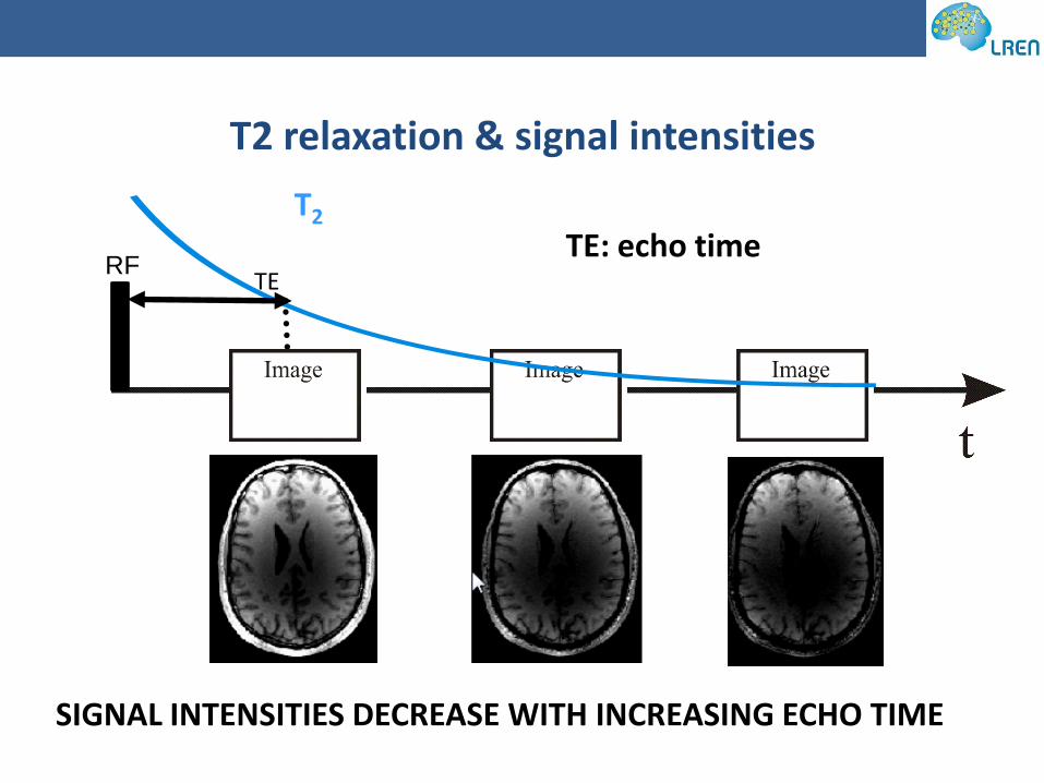
T2 relaxation & signal intensities
T2
TE
TE: echo time RF
SIGNAL INTENSITIES DECREASE WITH INCREASING ECHO TIME

T2 contrast
TE << T2 proton density-weighted image
TE RF
Image contrast is TE-dependent
TE ~ T2 T2-weighted image

Caudate Nucleus / GM (T2=100ms)
CSF (T2=2000ms)
Corpus Callosum / WM (T2=90ms)
37%
100%
Mxy
time
CSF
WM
GM
• T2,CSF>T2,GM/WM => On T2-weighted images, CSF appears bright
• WM and GM have similar T2 values => low WM/GM contrast in T2-weighted images
T2 contrast

Longitudinal relaxation
Return to equilibrium:
Increase of longitudinal component time constant T1
t
RF
M0 Ml
Mt
T1
The recovered longitudinal component will be flipped into the transverse plane when RF excitation is repeated

Longitudinal relaxation
19
t
RF RF
T1 relaxation during TR governs amount of magnetization available for next excitation
RF
Image Image
A simple imaging acquisition:
TR TR
T1 T1

WM
GM
CSF
T1 contrast
T1 differences between brain tissues yield image contrast in anatomical imaging
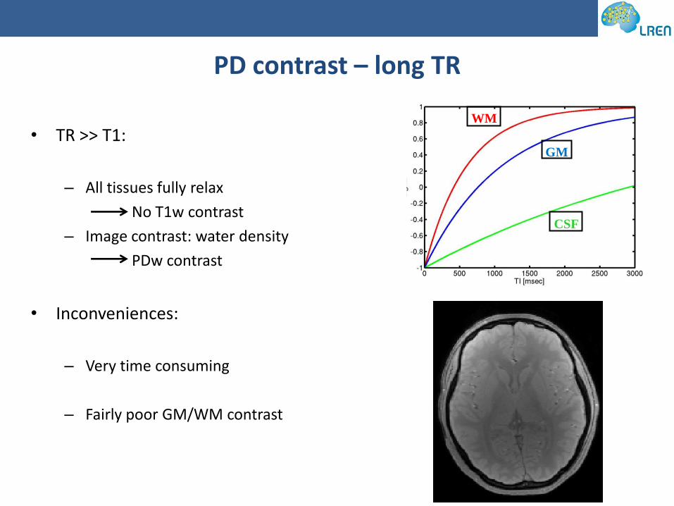
PD contrast – long TR
• TR >> T1:
– All tissues fully relax
No T1w contrast
– Image contrast: water density
PDw contrast
• Inconveniences:
– Very time consuming
– Fairly poor GM/WM contrast
WM
GM
CSF

T1 contrast – short TR
22
WM
GM
CSF
Frahm J. et al. MRM 1986
TR<<T1
Optimal GM/WM contrast Generally preferred for anatomical imaging

T1 contrast – short TR
t
RF (a) RF (a) TR TR=20ms
a=6o
PDw a=20o
T1w
WM
GM
CSF At short TR, image contrast depends on nominal flip angle of RF excitation

Anatomical sequences
• FLASH • Inversion Recovery (time consuming) • MPRAGE • MDEFT
FLASH MDEFT
Mugler & Brookeman MRM 1990; Mugler & Brookeman JMRI 1991 ; Look D.C., Locker D.R., Rev. Sci. Instrum, 1970 ;
Deichmann R. et al Neuroimage 2006
FLASH: ~6-7mins MDEFT:~12mins
Frahm J. et al. MRM 1986

Standard anatomical imaging applications
Ashburner & Friston Neuroimage 2000;
Anatomical images yields estimates of grey matter volume
Intracortical myelination Grey matter volume
Bartzokis G Neurobiol. Aging 2011

Standard anatomical imaging applications
Transient changes in brain structure due to juggling
Draganski B et al. Nature 2004
Standard anatomical imaging allows insight into brain plasticity
Perc
ent
chan
ge in
gr
ey m
atte
r

Improved morphometry: MT based VBM
Helms et al., Neuroimage 2009
MT > MDEFT
MDEFT MT
Grey matter volumes
Enhanced image contrast yields improved grey matter volume estimates
Image contrast
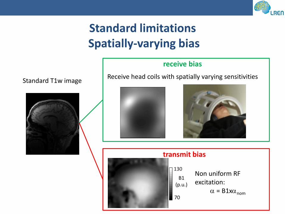
Standard limitations Spatially-varying bias
transmit bias
Standard T1w image Receive head coils with spatially varying sensitivities
receive bias
Non uniform RF excitation:
a = B1xanom 70
130
B1 (p.u.)
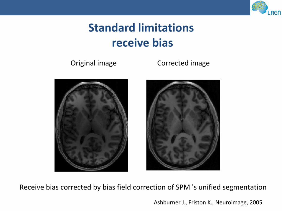
Standard limitations receive bias
Receive bias corrected by bias field correction of SPM 's unified segmentation
Original image Corrected image
Ashburner J., Friston K., Neuroimage, 2005

t
RF (a) RF (a) TR
T1 contrast – short TR
TR=20ms
a=6o
PDw a=20o
T1w Frahm J. et al. MRM 1986
Nominal value of RF excitation affects image contrast

Standard limitations transmit bias
• Non uniform RF excitation leads to inhomogeneous contrast over the image • Cannot be corrected at post-processing • Map of B1 field must be acquired in-vivo
70
130
B1 (p.u.)
Non uniform RF excitation:
a = B1xanom
Lutti A. et al MRM 2010, Lutti A. et al PONE 2012
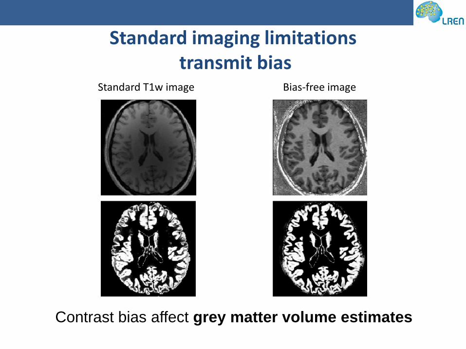
Standard imaging limitations transmit bias
Contrast bias affect grey matter volume estimates
Standard T1w image Bias-free image

Low sensitivity in cross-sectional/longitudidal studies
Mean
0 a.u.
800 a.u.
0%
20%
Inter-site variance
High variability across multiple scans – low comparability
Weiskopf N. et al Front. Neurosci. 2013
Standard imaging limitations comparability
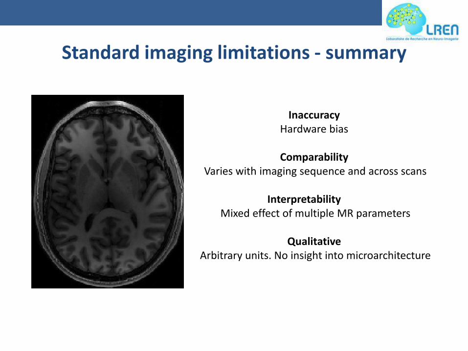
Standard imaging limitations - summary
Inaccuracy Hardware bias
Comparability
Varies with imaging sequence and across scans
Interpretability Mixed effect of multiple MR parameters
Qualitative
Arbitrary units. No insight into microarchitecture

Quantitative mapping - motivations
• Quantitative MRI provides quantitative and specific biomarkers of brain tissue properties (myelination, iron concentration, water concentration,...)
• No bias between brain areas (transmit/receive field)
Sereno M.I. et al., Cereb. Cortex 2013; Dick F. et al J. Neurosci. 2012
• Data quantitatively comparable across scanners. Optimal sensitivity in longitudinal and multi-centre studies

Quantitative mapping - motivations
Quantitative estimates of MRI parameters are biomarkers of tissue properties
Yao B. et al. NI 2009
Rooney W.D. et al MRM 2007
Macromolecular concentration

MPM protocol for quantitative mapping
Scan time: ~25min (1mm3 resolution) ~35min (800um3 resolution)
Helms G., et al MRM 2008; Helms G., et al MRM 2009; Lutti A. et al MRM 2010, Lutti A. et al PONE 2012;

VBQ: fingerprint of tissue changes in ageing
Draganski et al., Neuroimage 2011

Myelin mapping: towards in-vivo histology
Sereno M.I. et al., Cereb. Cortex 2013; Dick F. et al. J.Neurosci. 2012
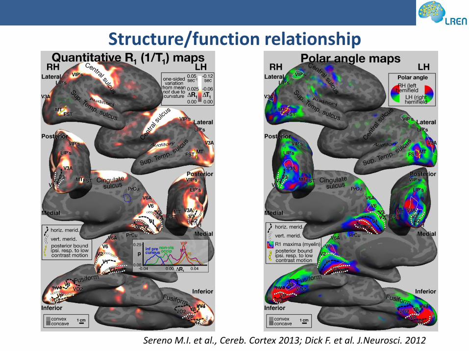
Structure/function relationship
Sereno M.I. et al., Cereb. Cortex 2013; Dick F. et al. J.Neurosci. 2012

Anatomical imaging - summary
Standard anatomical imaging
• Provides estimates of grey matter volumes. Study of brain plasticity, neurodegeneration,…
• Limited accuracy, sensitivity and specificity.
Quantitative MRI
• Provides quantitative estimates of MRI parameters
• Enhanced accuracy, sensitivity, specificity
• Provides biomarkers of tissue microstructure - insight into biological processes underlying tissue change.

Outline • General principals
– Origin of the signal
– RF excitation
– Relaxation (T1, T2, …)
• Anatomical imaging
– Image contrast
– Standard acquisition methods
– Advanced acquisition methods
• Functional imaging
– BOLD effect
– Limitations of fMRI acquisitions
– Advanced methods

Blood Oxygen Level Dependent (BOLD) effect • Ogawa et al., 1990: “static” BOLD effect in rat brain • Kwong et al., Bandettini et al., Ogawa et al., 1992: BOLD fMRI in human Note: localized changes, delayed/dispersed BOLD response
Kwong et al., PNAS 1992
Bandettini et al., MRM 1992

Magnetic susceptibility of hemoglobin
4x
Deoxygenated hemoglobin (Hb) • paramagnetic • different to tissue (H2O) • Changes local magnetic field and reduces signal in MRI images
Oxygenated Hb: • diamagnetic • same as tissue (H2O)
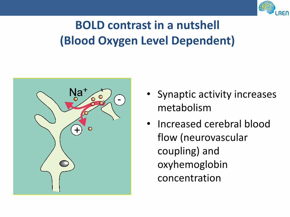
BOLD contrast in a nutshell (Blood Oxygen Level Dependent)
• Synaptic activity increases metabolism
• Increased cerebral blood flow (neurovascular coupling) and oxyhemoglobin concentration

The BOLD effect
Active Resting
venous
arterial
Oxygenated / deoxygenated hemoglobin = endogenous contrast agent
Echo time
active rest
MR Signal
BOLD EFFECT Change in oxygenated / deoxygenated hemoglobin concentration leads to detectable signal change

Functional imaging requirements
• Rapid sampling of BOLD response - Short acquisition time per image volume
'
111
22
*
2TTT
• Optimal BOLD sensitivity – T2* weighted contrast
t
Signal
T2
T2*
Field inhomogeneities
SP
Mm
ip
[25
.5, -9
0, -6
]
<
< <
SPM{T235
}
Left
SPMresults: .\Checkerboards\GLM\sub5Height threshold T = 3.125273 {p<0.001 (unc.)}Extent threshold k = 0 voxels
Design matrix
1 2 3
50
100
150
200
250
contrast(s)
2
0 100 200 300 400 500 600 700 800-6
-4
-2
0
2
4
6
8
10
12
time {seconds}
resp
on
se a
t [2
5.5
, -9
0, -
6]
Fitted responses
Left
fitted
plus error
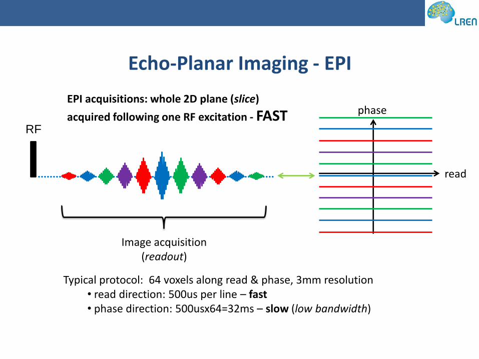
Echo-Planar Imaging - EPI
RF
read
phase
Image acquisition (readout)
Typical protocol: 64 voxels along read & phase, 3mm resolution • read direction: 500us per line – fast • phase direction: 500usx64=32ms – slow (low bandwidth)
EPI acquisitions: whole 2D plane (slice)
acquired following one RF excitation - FAST

Echo-Planar Imaging - EPI
t
RF
Image
TR RF
Image
TR RF
Image
TR RF
Acquisition time per volume:
TRvolume = Nslices x TR
Slice ordering: ascending, descending, interleaved
3mm resolution: TR~60ms

Echo-Planar Imaging - EPI
RF
readout
TE
Optimal echo time TE for fMRI
BS(TE) = C · TE · exp(-TE/T2*)
TE = T2* = 45 ms (at 3T)
At 3T TE = 30 ms: - Good trade-off between high BOLD sensitivity and low susceptibility-related signal dropout
- Optimal time-efficiency
Echo-Planar Imaging - EPI
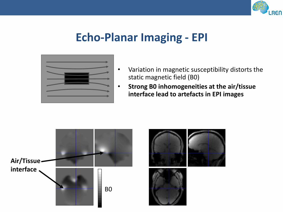
• Variation in magnetic susceptibility distorts the static magnetic field (B0)
• Strong B0 inhomogeneities at the air/tissue interface lead to artefacts in EPI images
Air/Tissue interface
B0

Susceptibility effects in EPI: distortion and dropout
t
Signal Homogeneous B0
Image
t
Signal Homogeneous B0
Image
Inhomogeneous B0
Strong B0 inhomogeneities
Full signal decay before image acquisition Signal dropout
t
Signal Homogeneous B0
Image
Moderate B0 inhomogeneities
Increased signal decay during image acquisition Image distortions

Susceptibility effects in EPI: distortion and dropout
Dropout
Distortion
Dropout and distortion
Phase-encode direction
Phase-encode direction

EPI distortion correction with field map
Jezzard and Balaban, 1995, MRM, 34(1);65-73; Hutton et al, 2002, Neuroimage, 16(1);217-240
B0 field Map of voxel displacements
Hz Pixels
Mapping of B0 inhomogeneities calculated from ‘fielmap data’
Fieldmap toolbox
Image processing

Use pixel shift map to unwarp image
EPI distortion correction with field map
B0 field Map of voxel displacements
Hz Pixels
Jezzard and Balaban, 1995, MRM, 34(1);65-73; Hutton et al, 2002, Neuroimage, 16(1);217-240
Mapping of B0 inhomogeneities calculated from ‘fielmap data’
Fieldmap toolbox
Image processing

Susceptibility effects in EPI: distortion
Cusack et al., Neuroimage 2003
• Distortion
– Pixel displacement in phase-encoding direction
– Problem for spatial localisation of activations.
– Inaccurate coregistration reduces sensitivity of group studies.
• Reduce distortion
– Shorter acquisition times, use parallel imaging
• Distortion correction
– Post-processing using field maps

• Use of preparation gradient pulses (zshim gradients) to compensate local dropouts
• But: Reduces signal in normal areas
Acquisition of several images with different z-shimming reduces temporal resolution Optimal compromise: moderate zshimming
Dropout compensation: z-shimming
Frahm et al., MRM 1988; Ordidge et al., MRM 1994
No z-shim
With z-shim

(Simulation for slice thickness of 2 mm)
z-shimming with -2 mT/m*ms No z-shimming
Normal
Orbitofrontal Orbitofrontal
Normal
Moderate z-shimming: trade-off
Deichmann et al., Neuroimage 2003

Standard EPI BS
10
20
30
40
50
60
Moderate z-shimming: example
EPI + z-shim

Dropout compensation - multi-echo EPI
• Acquire multiple EPI readouts (=images) after a single RF excitation pulse
• Short TE images recover dropouts
Poser et al., Neuroimage 2009
• Enhanced BOLD sensitivity over the whole brain
• Pitfall: increased acquisition time
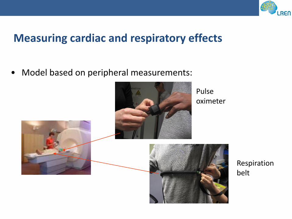
Measuring cardiac and respiratory effects
• Model based on peripheral measurements:
Pulse oximeter
Respiration belt

Modelling and correcting for cardiac and respiratory effects
• Measured cardiac and respiratory phase can be modelled using a sum of periodic functions e.g. sines and cosine of increasing frequency (Fourier set)
Glover G.H. Et al. MRM 2000; Hutton et al., Neuroimage 2011
• Modelled effects can be
– removed from original fMRI signal
or
– included in fMRI statistical model
Cardiac, respiration,…
Interest
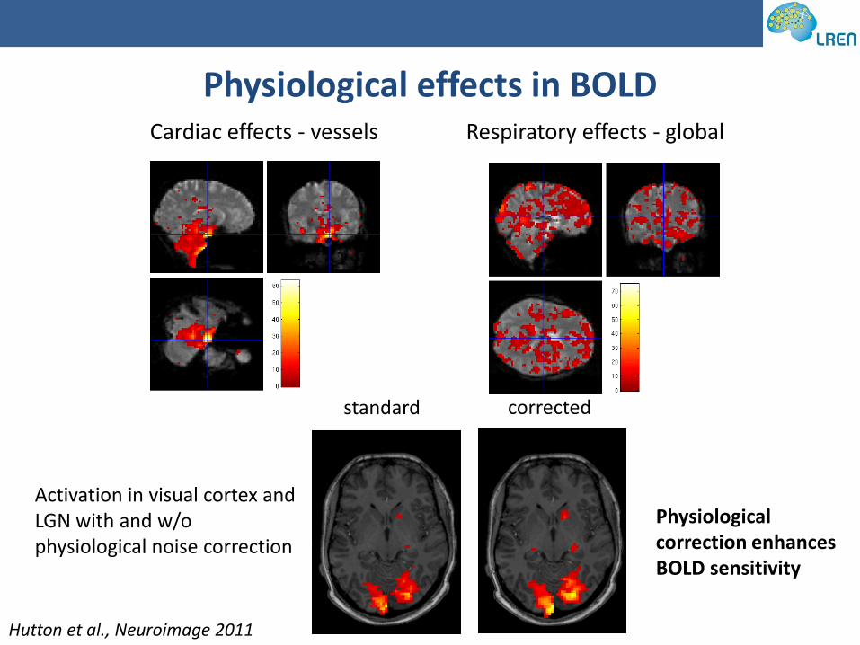
Physiological effects in BOLD Cardiac effects - vessels Respiratory effects - global
corrected standard
• Activation in visual cortex and
LGN with and w/o physiological noise correction
Hutton et al., Neuroimage 2011
Physiological correction enhances BOLD sensitivity

3D EPI acquisitions for fMRI
Krueger, G., Glover, G.H. MRM 2001, Triantafyllou, C. et al Neuroimage 2005
3D EPI yields higher image signal-to-noise (SNR0)
Temporal stability (tSNR) is an indicator of BOLD sensitivity
tSNR vs SNR0

tSNR3D - 128% tSNR2D in VC - 164% tSNR2D in LGN
2D
3D
Temporal SNR
50
0
50
0
High-resolution EPI: 1.5mm 2D/3D EPI at 3T
Lutti et al., Magn Reson Med 2013

3D EPI acquisitions for fMRI
Krueger, G., Glover, G.H. MRM 2001, Triantafyllou, C. et al Neuroimage 2005
3D EPI yields higher image signal-to-noise (SNR0)
Temporal stability (tSNR) is an indicator of BOLD sensitivity
tSNR vs SNR0

Ultra-fast fMRI - 3mm3 resolution
• Dual-echo whole-brain EPI acquisition
• Matrix size: 72x64x60 (PExROxPA)
• Acceleration factor 2 and 3 along the phase and partition directions
• TR = 1s
Echo1 TE=15.85ms
Echo2 TE=34.39ms
Echo1 +Echo2
Poser B.A., Norris D.G. Neuroimage 2009;
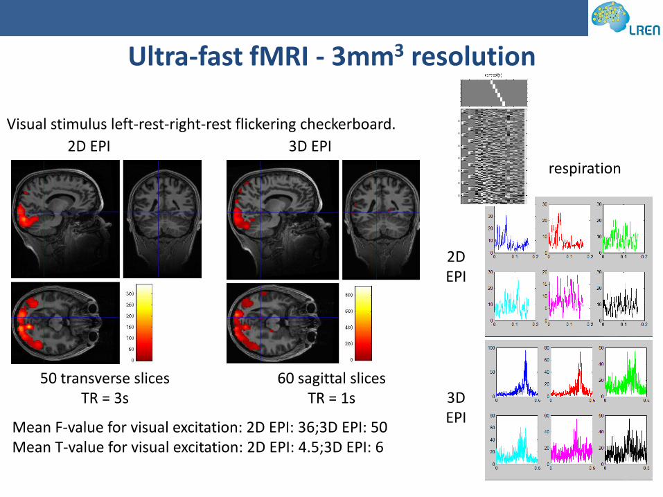
Ultra-fast fMRI - 3mm3 resolution
Visual stimulus left-rest-right-rest flickering checkerboard.
2D EPI 3D EPI
50 transverse slices TR = 3s
60 sagittal slices TR = 1s
Mean F-value for visual excitation: 2D EPI: 36;3D EPI: 50 Mean T-value for visual excitation: 2D EPI: 4.5;3D EPI: 6
respiration
2D EPI
3D EPI
Functional imaging - summary
• fMRI: brain activation detected via increased metabolim (‘BOLD effect’)
• EPI acquisitions allow optimal sampling of BOLD response
• EPI images/time-series:
– Distortions – corrected at post-processing
– Signal dropouts –minimized at run time
– Physiological instabilities - online monitoring + offline processing
• Advanced acquisitions:
– Enhanced BOLD sensitivity – high resolution
– Rapid acquisitions – higher efficiency
Correction yields optimal BOLD sensitivity