The Urban Transportation

Planning Process

March 23, 2003 Version

Robert A. Johnston

University of California, Davis

Introduction

The rapid movement of people and goods is essential to economic growth in the U.S. and

in every one of its urban areas. Funds for building and operating highway and transit systems are

a major fraction of expenditures for local, state, and Federal governments. Traffic congestion is

one of the most important issues facing local elected officials everywhere. Suburbs fight for

more highway funds, while central cities push for transit improvements. In all large urban

regions, these jurisdictions must cooperate in regional transportation planning exercises, every

three years.

Urban transportation planning in the U.S. began with the development of travel demand

models in the 1950s and then became formalized in the 1960s with the U.S. Department of

Transportation (USDOT) codifying practice and software. Travel models take regionwide 20-

year projections of future land uses in small zones and convert these into numbers of households,

1

which generate trips, and employees, which attract trips. With computer software, the trips are

assigned to a network of roads that connects the zones. As more trips are loaded onto the

network, travel speeds slow down and some trips are assigned to faster sets of links in the

network. After many iterations where all trips try all possible routes, total traveler time is

minimized. Then, travel speeds on the links are analyzed to see where congestion is the worst.

These congested areas are where additional investment will be needed, to increase road or transit

capacity.

In this chapter, we will begin by reviewing the history of regional transportation planning

in the U.S. Next, we will identify recent Federal laws that place additional requirements on

transportation modeling and planning. Then, we provide a detailed review of the steps in travel

modeling, outlining improvements being undertaken by the larger agencies. Then, we review the

great variety of policy analysis capabilities that are now being taken on by regional

transportation planning agencies, due to the needs of citizens groups and of local governments.

These are the “bottom-up” needs that come from the constituent groups, in addition to the “top-

down” requirements from the Federal laws. This review is followed by the outline of an

ambitious model improvement program in one region, to bring all of these pieces together.

Finally, we describe foreseeable future modeling advances , so that the reader will be able to

anticipate practice during the next decade.

History of Regional Transportation Planning

Regional transportation planning is required for medium-sized and large urban areas, in

order to qualify for Federal highway and transit funding. Many states also have similar

requirements, to get state funding. Transportation is the only remaining type of infrastructure

2

funding for which Congress still requires regional planning. Such planning was formerly

necessary to apply for Federal funding for hospitals, sewage treatment plants, and water supply

systems, but these regulations were dropped in the 1970s (OMB Circular A-95). Regional

transportation planning is a vital arena to understand, both because it is the only regional

planning process undertaken regularly in most regions, but also because changes in

transportation systems can affect not only traffic congestion, but also air quality, transit

availability for lower-income households, and land development patterns.

Before World War II, transportation planning did not include travel modeling. After the

War, rapid increases in automobile ownership, widespread suburbanization, and a vast increase

in Federal spending for transportation investments led to the need for regional modeling of travel

behavior. Early studies were done in Detroit and Chicago, followed by studies in other Eastern

cities. Many of the early methods were developed by the Chicago Area Transportation Study.

The Federal Highway Act of 1963 required urban areas to use a “continuing, comprehensive, and

cooperative” transportation planning process (the 3C process), to qualify for Federal funding.

Urban areas were defined as regions and so regional modeling became the standard procedure.

The Bureau of Public Roads (later, Federal Highway Adminstration) sponsored research to

develop standardized methods and published manuals describing travel modeling methods and so

practice became standardized nationwide. Specifically, these methods became codified in the

Urban Transportation Modeling System (UTMS), or Urban Transportation Planning System

(UTPS), which was a standardized set of methods for "four-step" travel modeling: trip generation

(number of daily household trips), trip distribution (where each trip goes), mode choice (which

travel mode is chosen), and route assignment (routes on roads, rail lines, or bus lines). Many

regions used the software disseminated by USDOT, for use on mainframe computers.

3

We need to outline how travel models are designed, as they play a central part in

transportation planning. First, the Metropolitan Planning Organization (MPO) divides the region

into a 100-2,000 zones, generally composed of block groups and census tracts. The agency

develops a set of networks in the travel model software that represent all the major roads and all

transit lines. Then, the MPO performs a household travel survey, where a few thousand

randomly selected households are surveyed on a random mid-week day, in order to identify all

trips made by time, mode, route, destination, and purpose. These data are then used to estimate

several submodels, also known as the travel model steps.

An ideal travel model would repesent all behaviors affected by changes in the

transportation system. The model would be estimated on large datasets and the equations in the

various submodels would have high explanatory value, statistically. Futhermore, the models

would include explanatory variables relevant to all major policy issues, such as road tolls, new

road capacity, and compact growth.

Travel models are composed of four main submodels. The MPO estimates a Trip

Generation model where household characteristics (income, size, others) determine the number

of trips made per weekday. Second, a Trip Distribution model is estimated, where trips are

generated by households and attracted by employment. The trips are linked randomly from one

zone to another and then a proportionate fitting program rematches origin and destination zones,

to get a distribution of trip time lengths that matches that in the survey data. This is done

separately for each trip purpose (Home-Based Work, Home-Based Other, Non-Home-Based are

the minimum set). Then, the agency estimates a Mode Choice model, where the travel mode

chosen is a function of the modes available to the household, household income, and the cost of

the mode for each trip taken (time cost plus auto mileage costs or transit fares). Finally, in the

4

Assignment step, trips are assigned to the network, to get from the origin zone to the destination

zone. As links become loaded, the vehicle speeds slow down. This results in some trips being

assigned to other routes, until no trip can be made faster.

Each submodel can be calibrated (forced) to other data sets, often data from the survey

that was partitioned out and not used for model estimation. Then, the whole model set is run on

the base year data and traffic volumes are calibrated to actual traffic counts in certain parts of the

region. Various adjustments are made in the submodel parameters until the modeled traffic

volumes match the observed volumes fairly well. This calibration is also done for transit line

ridership for all transit lines and for regional mode shares and number of trips. After the model is

calibrated, it is run for those future years of interest, based on projected population and

employment. Generally, models are run on a 20-year horizon, for facility planning, and are also

run on intermediate years for which there is a vehicle emissions reduction deadline.

In the 1960s, opposition to freeways in central cities resulted in a statutory requirement

for a local freeway agreement to be signed by all cities and counties where the right-of-way

would be acquired. Rising environmental concerns led to the adoption of NEPA, the National

Environmental Policy Act, in 1969, which requires a detailed environmental assessment of all

Federally funded projects. In 1975, the U.S. Department of Transportation (USDOT) adopted

regulations requiring not only a long-range (20-year) plan, but also a short-term element,

focusing on low-cost Transportation Systems Management (TSM) policies, such as carpool

lanes, ramp metering, and limiting parking. These measures were to reduce peak demand and to

better manage peak flows, and so represented the first Federal objectives for demand

management, not simply providing more capacity on roads and transit lines. Also, public

5

participation requirements were strengthened and attention was to be paid to the transportation

needs of the elderly and poor.

In the early 1980s, the Federal agencies reduced their oversight of regional planning

somewhat, but the basic planning requirements stayed in place. Federal funding for new freeway

and highway capacity began to decline steadily as the Interstate System was almost completed.

Greater suburban travel and higher auto ownership in general led to continuing rapid increases in

vehicle miles of travel (VMT), a broad measure of travel demand within urban regions. Although

tailpipe controls on vehicles continued to improve, still the vast majority of larger urban regions

did not meet all Federal air quality standards. Many urban regions adopted plans with light rail

systems and, in general, there was an increased interest in transit improvements, some of this

directed to urban renewal objectives for central cities.

In the 1950s and 60s, travel modeling addressed mainly the simple issue of where to

provide new freeways and highways. This problem merely requires the agency to determine the

most congested corridors in the road system. Only the trip distribution step (where do trips arise

and to where do they go) and route assigment model step have to be roughly right, to determine

relative congestion levels on roads. Trip generation and mode choice do not have to be very

accurate. Models were generally daily models, that is they represented all daily travel. Peak

vehicle flows were simply factored (as about 10% of daily trips in the peak hour). Vehicle speeds

were very poorly simulated. Travel models were generally accurate enough for ranking network

links by congestion level, however.

In the 1970s and 80s, travel modeling practice advanced statistically, with the use of

disaggregate discrete choice models, mainly for mode choice, advocated at the Williamsburg

Urban Transportation Modeling Conference, held by USDOT in the early 1970s. There have

6

been international travel modeling conferences every few years since then, focusing on making

travel models more behavioral and accurate. There are a great many consulting firms that are

competent in discrete choice model development. Smaller urban areas with, say, less than

200,000 people, still generally do not use mode choice models, but regions above this population

do, as they have significant bus and rail systems, or wish to plan for them.

Let us now review recent Federal laws that greatly increase the requirements placed on

travel modeling and on transportation planning. Agencies are still trying to adjust to these new

mandates. Whereas in the 60s, 70s, and 80s the Federal government was primarily

concerned about congestion reduction from transportation investments, in the 1990s air

quality concerns became equally important.

PAS FIGURE 3.3 HERE?

Recent Federal Planning Requirements

The Clean Air Act of 1971 required all states to adopt a State Implementation Plan (SIP)

that includes an emissions inventory for each region in the state and a plan for attainment of all

ambient Federal air quality standards. The Clean Air Act amendments of 1977 and the

subsequent Highway Act both required all regional transportation plans to show attainment of

the vehicle emissions reductions specified in the SIP, through the modeling of travel and

7

emissions from on-road vehicles. The emissions modeling is governed by the US Environmental

Protection Agency (USEPA) and most states use the EPA emissions modeling software. This

program takes daily VMT (in each vehicle speed class) data for the region (taken from the travel

model), and other data such as number of trips, and produces emissions projections. It also relies

on vehicle fleets specified by the EPA for all future years (number of vehicles by model and

year). Under the 1977 amendments, a region that did not do a transportation plan could have its

Federal funds for transportation improvements denied (the “funding sanction”).

The Clean Air Act of 1990 is the most important policy advance in transportation

planning in recent decades. It greatly strengthens the previous requirement for air quality

attainment, by providing that Federal transportation funds can be withheld from regions that

adopt transportation plans, but cannot show attainment (through modeled emissions reductions)

by the deadlines for each pollutant. This was the first time the funding sanction had been tied to

actual attainment, and so represents a much stronger incentive for regions to reduce emissions.

The Clean Air Act of 1990 also strengthens the role of demand-side policies, by requiring that

Transportation Control Measures (TCMs) be studied in nonattainment regions and lists the

TCMs that must be studied for each level of nonattainment (moderate, serious, severe, and

extreme). The TCM lists included much stronger demand reduction policies than had appeared

on the earlier lists of TSM policies. TCMs, for example, include peak-period road tolls.

The Surface Transportation Act of 1991 reinforced the policies in the Clean Air Act of

1990 and emphasized multi-modal planning (for all modes, in a connected system). It also

strengthened the requirements for public participation and interagency consultation and required

that MPOs with over 200,000 populations have their planning procedures recertified by USDOT

every three years. The objectives of transportation planning have evolved from adding road

8

and transit capacity to also managing travel demand, connecting modes, and reducing

emissions.

The Clean Air Act air quality conformity rule, adopted pursuant to the Act, requires that

all regions with serious or worse ozone or carbon monoxide nonattainment status run models that

are equilibrated across all model steps, to fully represent the effects of changes in accessibility on

travel demand (40 CFR 93.122(b)(1)). The long-time contention by academics and

environmental groups that adding capacity speeds up travel and so people make longer trips

resulted in this modeling rule. There is considerable evidence for this behavior where increased

accessibility on roads leads to increased travel (Expanding Metropolitan Highways, 1997;

Cervero and Hansen, 2000). Most larger Metropolitan Planning Organizations (MPOs) have now

begun to run their travel models in this fashion. Equilibrated, or “full feedback” modeling means

that the speeds in the Assignment step are fed back to the other model steps.

The conformity rule also requires that the land development effects of regional

transportation plans be accounted for, in the serious and worse air quality regions. It says that the

land use patterns and facility plans must be “consistent” in each alternative (40 CFR 93.122(b)

(1)). This is a much more contentious rule, as it requires MPOs to adopt some sort of land use

forecasting committee or model. Due to a lawsuit in the Chicago region in the mid-90s and to

this rule, most large MPOs are now developing land use models to run in combination with their

travel models. Medium-sized MPOs with serious or worse air quality are beginning to do the

same. MPOs do not regulate land use and so they must gain the cooperation of their member

cities and counties to allow alternative land use projections to be run with each regional

transportation (facility) plan.

9

More fundamentally, the Clean Air Act of 1990 requires the MPO modeling in these

regions to be much more accurate, so that emissions will not only be ranked correctly across

alternative plans, but also be projected accurately absolutely, in order to judge the performance

of any plan against emission reduction budgets developed for each nonattainment region. This

means that travel must be projected by time of day (peak and off-peak periods), to forecast

congestion, vehicle speeds, and emissions in more detail. Travel speeds must also be much more

accurate than in the past. Most large, and some medium-sized, MPOs now use speed post-

processors (extra models) to project vehicle speeds more accurately. These models are calibrated

against observed vehicle speeds, in the base year model. Air quality conformity must be

demonstrated every three years, in each transportation plan. This new level of modeling accuracy

is very difficult for MPOs to achieve.

In addition, the Clean Air Act of 1990 requires that all MPOs be able to model the

effects of Transportation Control Measures such as peak-period tolls, parking charges, fuel taxes,

flextime, paratransit, transit, land use intensification near to rail stations, bike and pedestrian

facilities, park-and-ride lots for transit and for carpooling, ramp metering, and carpool lanes.

This requirement means that the travel model must be sensitive to a much greater variety of

policies and travel behaviors than in the past. Models need to represent all transit and walk and

bike modes, for example. They also must include prices for travel (time cost, distance cost,

transit fares and tolls and parking charges) for all modes, in all model steps. The more advanced

large MPOs’ models do include all of these variables to make them sensitive to such policies, but

the medium-sized MPOs need to catch up by adopting substantial model improvement programs.

The Civil Rights Act of 1964 has resulted in a series of transportation discrimination

cases that are making MPOs consider the equity effects of their plans more seriously. A very

10

important settlement in Los Angeles County in the 1990s, for example, requires much greater

investment in bus system improvements, because poor people ride buses, not rail. The MPO for

that region now includes simple equity measures in its regional plans. The 1998 EPA Guidelines

on Environmental Justice are being implemented by all Federal transportation agencies. Some

states also have adopted their own statutes requiring the analysis of such equity issues. It is worth

noting that, to get theoretically complete economic equity measures, you have to run economic

models within your travel model or land use model. This is the least understood and least

developed area of MPO practice, even though such models are in widespread use in other

developed countries.

In some regions, NEPA is increasingly being enforced (through lawsuits) regarding the

growth-inducing impacts of highways. The MPOs will need to model induced travel (VMT) and

induced land development (type and location) for major road and passenger rail improvements.

Since cities and counties control land use planning, MPOs often treat these projections of land

development as “impact evaluations,” not land use plans.

One useful way to think of all of these requirements for modeling is list all of the

behaviors we wish to simulate. In conventional travel models these behaviors are only crudely

represented:

1. Trip generation is represented poorly. Nonmotorized modes are omitted, only a few trip

purposes are identified, and there are no land use and accessibility explanatory variables. This

means the effects of land use density on trip generation are not modeled and the effects of land

use policies on walking and biking are also omitted, for example.

2. Trip distribution (specifying the number of trips from each residence zone to each workplace

zone) is rudimentary. Trips are not linked in sequences, but are all modeled separately. Workers

11

from households are not matched to job types by income. The monetary costs of travel are not

represented. The whole model set is not run to equilibrium, and so the effects of vehicle speeds

on trip lengths is neglected.

3. Mode choice, at least in the larger MPOs, is done fairly well with disaggregate models.

Nonmotorized modes are missing, in most models, however. Small MPOs omit this step. Some

of them use “trip diversion” curves to project transit shares.

4. Travel assignment is quite inaccurate, as road capacities are often inaccurate and the relation

between vehicle flows (road volumes) and speeds are poorly represented. Generally, quite

inaccurate speeds result, especially in daily models. As a consequence, projected congestion

levels are unreliable. Emissions estimates are, therefore, inaccurate.

Behaviors that are generally missing completely (for which new submodels must be

created) include:

1. Auto ownership (autos per household), which strongly affects trip generation and mode

choice.

2. Trip chaining, which increases as congestion gets worse (drivers link more trips together).

Chaining also reduces the number of cold engine starts, which are a critical input to an emissions

model.

3. Time of travel, which is affected by congestion. Peak spreading occurs, as congestion

worsens, and this affects speeds and emissions (more people travel at shoulder times and off-

peak times).

4. Location of land development, which is affected by congestion levels in subareas in the

region.

12

5. Location of firms. As congestion levels change, firms move around in the existing building

stock, to be close to their workers, suppliers, and customers.

6. Location of households. As congestion changes, households move around in the available

dwellings, in order to have access to employment, shopping, and schools.

To summarize, MPOs are now required to greatly improve their capabilities for

modeling travel and land development and the effects of the resultant travel and land use

patterns on the economy, environment, and social equity.

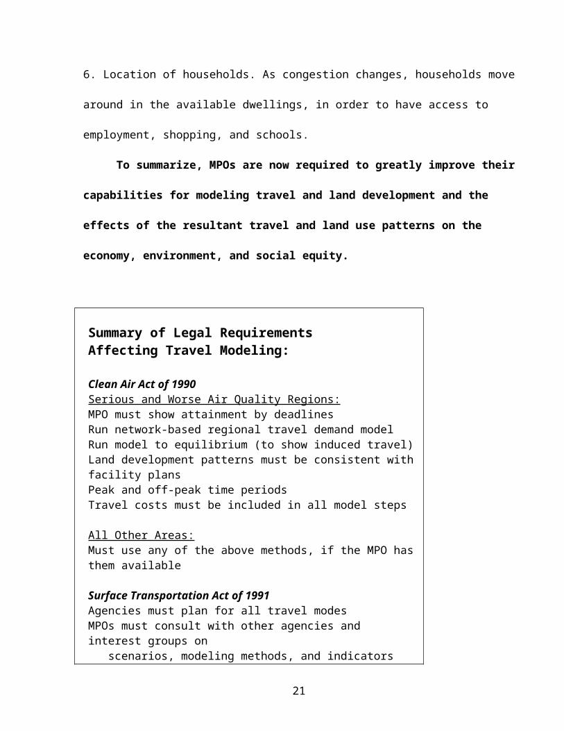
Summary of Legal RequirementsAffecting Travel Modeling:

Clean Air Act of 1990Serious and Worse Air Quality Regions:MPO must show attainment by deadlinesRun network-based regional travel demand modelRun model to equilibrium (to show induced travel)Land development patterns must be consistent with facility plansPeak and off-peak time periodsTravel costs must be included in all model steps

All Other Areas:Must use any of the above methods, if the MPO has them available

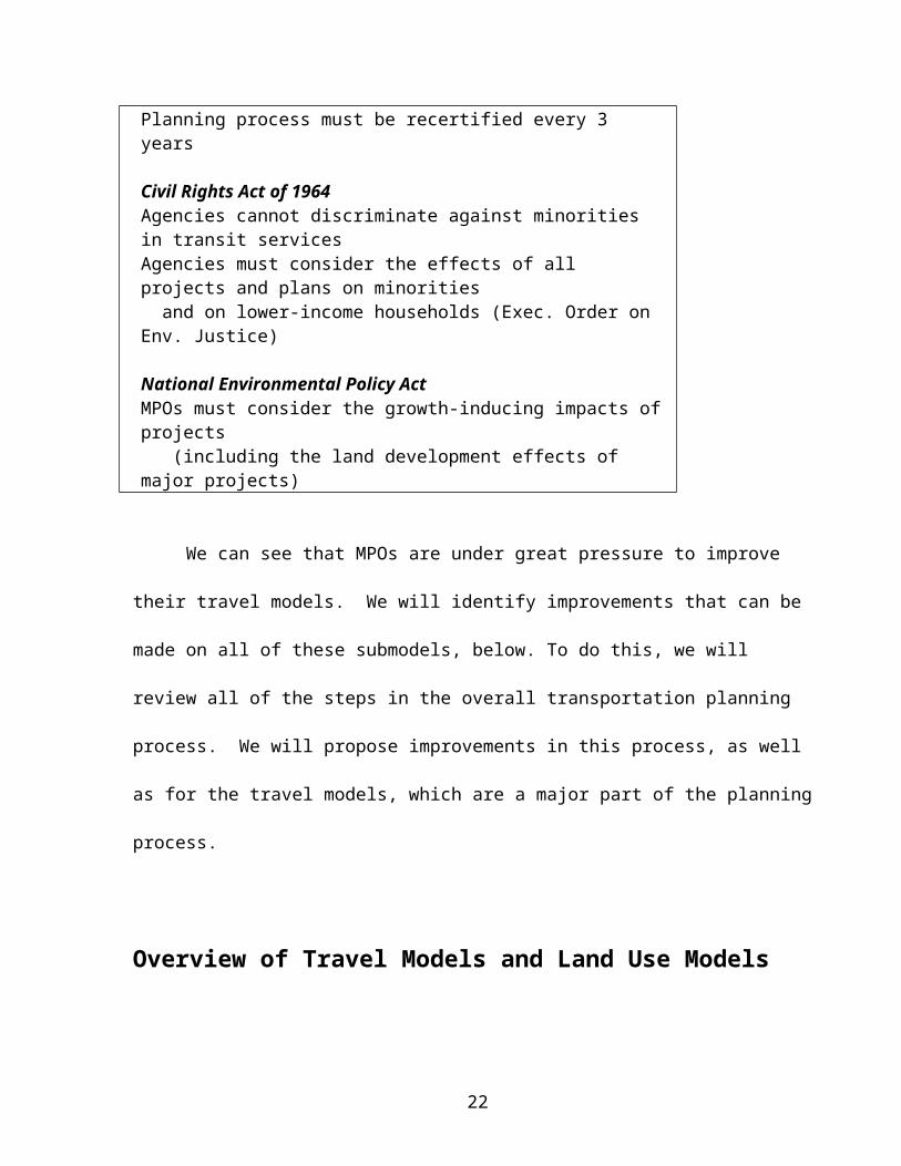
Surface Transportation Act of 1991Agencies must plan for all travel modesMPOs must consult with other agencies and interest groups on scenarios, modeling methods, and indicatorsPlanning process must be recertified every 3 years

Civil Rights Act of 1964Agencies cannot discriminate against minorities in transit servicesAgencies must consider the effects of all projects and plans on minorities and on lower-income households (Exec. Order on Env. Justice)

National Environmental Policy ActMPOs must consider the growth-inducing impacts of projects (including the land development effects of major projects)

13

We can see that MPOs are under great pressure to improve their travel models. We will

identify improvements that can be made on all of these submodels, below. To do this, we will

review all of the steps in the overall transportation planning process. We will propose

improvements in this process, as well as for the travel models, which are a major part of the

planning process.

Overview of Travel Models and Land Use Models

Following Pas (1993) we will divide the planning process into three phases and describe

past practice. Drawing from Beimborn and Kennedy (1996), Deaken, Harvey, and Skabardonis

(1993), and the recent model development programs for Oregon and the Sacramento region, we

outline the improvements generally agreed-on for medium-sized and large MPOs, at the end of

each section. We will not discuss goods movement, due to limited space. Other good sources

include Summary of Comments (1994) and Johnston and Rodier (1994). The best recent set of

recommendations for travel models and land use models is Miller, Kriger, and Hunt (1999).

Pre-Analysis Phase

The Pre-Analysis Phase consists of: 1. problem identification, 2. formulation of

objectives, 3. data collection, 4. generation of alternatives, and 5. definition of evaluation

measures. The most important aspect of this phase is to define problems broadly and then

identify broad objectives. In this way, many solutions can be sought, not just road capacity

increases. So, rather than an objective of “Widen congested roadways,” an MPO should define

the objective to reduce congestion as “Maximize accessibility in the region, especially for lower-

income households.” This definition focuses on those travelers with few options and so

14

encompasses equity. This is preferable to defining a second objective for equity, which can be

downplayed in the analysis. My definition also states the problem as accessibility, not improved

level-of-service (speeds) on roads, because higher speeds results in higher VMT (which then

increases emissions). Accessibility is simply access to activities, which are the good being

sought by the traveler. Travel is primarily a means to get to activities, such as work and

shopping, or visiting friends, not a good in itself. So, we can increase accessibility with a policy

for higher-density mixed-use land use centers, by themselves or with better transit. More freeway

capacity will also increase accessibility, and so this definition is mode-neutral. Given the broad

policy charge in the most recent transportation acts and the need to examine TCMs in the air

quality law, we need to define transportation planning objectives in a holistic fashion, in order to

not bias our studies.

The generation of alternatives is another especially weak step in transportation planning.

Most MPOs initially analyze several roadway and transit investment schemes, but do this in-

house, not in published documents. In the official plan, the MPOs usually analyze only the

Preferred Plan and the No Action Alternative, which is required by NEPA. The preferred plan, in

many instances, seems to be the maximum investment in roads where the plan can just meet the

future emissions requirements. Transit is added to reduce emissions, as necessary, and to satisfy

interest groups advocating for transit and for lower-income households in general. MPOs almost

never identify and evaluate all-transit alternatives (the author has reviewed most of the plans

from the largest 15 MPOs). The main reason for this appears to be that transit investments will

generally focus on the central cities in a region and so will not meet the chief political test of

MPO decisionmaking, which is geographic equity (spreading the money around). Each MPO

board member is an elected local government official and so he or she wants to bring the dollars

15

into their jurisdiction. In some states, such as California, transportation funds are legally

allocated by population, and so outlying counties get their “share” of funds. These funding rules

make transportation planning more a process for spreading projects around than one of seeking

to meet regional objectives for economic efficiency, equity, or even congestion reduction. This is

a good example of how “planning is politics.” Nevertheless, it is very important for MPOs to

examine several alternative plans, including ones that focus on transit and land use in central

cities, as well as on typical freeway widenings, to see the results. Several MPOs have engaged in

visioning processes over the last 20 years, where they examined broadly different alternatives,

projected for 40 or 50 years. This is an essential part of transportation planning and should be

done every ten years or so by MPOs, outside of the regular planning cycle. These broad analyses

may affect the funding process in ways that benefit the whole region.

The third weakness in this phase is inadequate plan evaluation criteria. Travel models

output measures of congestion, such as level-of-service (A – F) on each network link and person-

hours of travel delay. They also send their VMT-by-speed-class projections to emissions models

that output tons of each pollutant per weekday. MPOs, however, seldom evaluate equity

outcomes well and they seldom evaluate aggregate economic welfare at all. These measures are

urged, but not required by, the Surface Transportation Act of 1991. They are, however, essential

to an informed and accountable planning process. There are easily applied measures of

comparative aggregate economic welfare (net benefits to travelers). These measures can come

directly from the mode choice model, or for smaller MPOs without such models, from travel

costs calculated off-model using travel times and distances from the travel model. These

measures can also be calculated for travelers by income class and so can give a vertical equity

measure (economic welfare by household income class). Since few MPOs in the U.S. use these

16

measures, economic welfare and social equity are not given much weight in plan evaluation.

Such measures are used in most developed countries and in many developing ones. They are

required by multilateral banks, for major transportation investments.

Last, ongoing data collection is fundamental to accurate travel modeling. All MPOs

should perform a household travel survey every decade, coordinated with the national census. In

addition to travel questions asked of a random sample of the whole region’s population, surveys

can be done on the same households over time (panel surveys), and surveys can be used to

support land use modeling by asking questions about household and firm locational behavior.

One should also survey firms to determine goods movements, by commodity type. MPOs need to

perform a survey of employment, to supplement national sources such as InfoUSA. If an MPO is

going to develop a land use model, then it must also gather land use data. Most MPOs now have

geographic information system (GIS) capabilities and so can use parcel datasets, if all of their

constituent counties have these data. Parcel data, supplemented with airphotos and satellite data,

are the only way to get spatially accurate land use maps. All of these data gathering efforts are

expensive and time-consuming and so each MPO needs to have a model development program

where the data gathering and cleaning is part of an ongoing process.

In general, these issues of narrow objectives, narrow range of alternatives, inadequate

evaluation criteria, and insufficient data gathering are a consequence of inadequate MPO budgets

for transportation planning. MPOs that spend a $1 billion per year on transportation projects will

spend only a few million $ on transportation planning, which is a few tenths of a percent of the

budget. Private firms spend a much greater proportion of their overall costs on planning. Federal

funding rules permit the use of several categories of funds for MPO planning, but most MPOs

17

prefer to spend those funds primarily on facilities. This generalization, that MPOs don’t spend

enough on planning in the Pre-Analysis Phase, applies to the next two phases of planning, also.

Put Pas Figure 3.1 here?

Technical Analysis Phase

The next phase of transportation planning is the Technical Analysis Phase, which is

primarily the travel modeling, but may also include a land use model. Above, we noted that a

complete set of models would represent all behaviors n the urban system that are affected by

changes in the transportation system. Now, we will define an ideal model in more detail, from

the perspective of urban modeling, where all urban systems are represented. According to

Wegener (1994), urban models should represent all subsystems. He defines these systems by the

speed with which they change. Slow change systems include transportation networks and land

uses (permitted economic activities). Medium-speed change systems include workplaces and

housing, by which he means the construction of buildings. Fast change systems include

employment and population, meaning the movement of workers and households among existing

18

buildings. Immediate change systems include goods transport and personal travel. It is widely

accepted that changes in the transport networks will affect travel and goods movement and,

subsequently employment and population locations, and, finally, the construction of workplaces

and housing. This broader urban modeling perspective is now becoming accepted in

transportation planning and modeling When USDOT had four teams of consultants develop

outlines of advanced travel forecasting models in the early 1990s, three of the proposals included

land use models as part of the package, to ensure accuracy of travel forecasts (New Approaches

to Travel Forecasting Models, 1994).

With this broader perspective, let us now review again the typical MPO travel modeling

process, derived from the 1960s and still in use today, called the “four-step” modeling process.

This typical process does not include a land use model.

In recent years, there have been several conferences and publications calling for

improved travel models and for the addition of land use models to MPO practice. A compilation

of recommendations from peer reviews of travel models, done during MPO recertifications, was

published in 1993 (Peer Review, 1993). This report lists desirable modeling characteristics for:

observed data, demographic and economic forecasts, model system design, general forecasting

issues, trip generation, trip distribution, mode share, assignment, and other details. USDOT

published Short-Term Travel Model Improvements in 1994. Good papers from this period were

by Stopher (1993a, b) and Deakin, Harvey, and Skabardonis (1993). Hundreds of papers have

been published and presented at the Transportation Research Board annual meetings, over the

last 20 years on how to improve travel models.

Activity Forecasts. These forecasts are done before the four-step model is run. The MPO

needs data on households and employment for the base year and for the forecast years. Base year

19

data are gotten from the national census and from the MPO’s household travel survey and other

local surveys and GIS datasets (census: households, number of workers per household, persons

per household, household income, number of autos per household, all by zone; other data

sources: number of employees by type of employment by zone). Then, population and

employment forecasts for the counties in the region are taken from a state agency. These are

usually derived from national and state input-output and econometric models of the national and

state economies. We will not concern ourselves with the accuracy of these projections, since they

are exogenous, except to note that the error is, on average, at least one percent for each year of

the forecast, meaning that the typical 20-year projections can be high or low by 20% or more. In

addition, the MPO must get or make forecasts for household income and size, the other most

important variables in the travel model. Many states provide these forecasts for counties. Errors

in demographic inputs to travel models are unavoidable. This is one reason that MPOs are

required to redo their transportation plans every three years.

The MPO then must distribute the firms and households to zones. This is usually done for

a few hundred to two thousand travel analysis zones (TAZs), which are generally the base year

block groups or census tracts. Only a few large MPOs use some sort of land use model to

allocate households and firms to zones in future years. The vast majority of MPOs use a

judgemental process where the staff examines vacant lands in each county and what the land use

designations are for them in each county’s land use plan. By hand, or using a simple GIS system,

the MPO staff assigns future households by density class and income (income correlates with

density and with existing incomes). Future household auto ownership level generally is also

correlated with existing auto ownership, which comes from census data. Types of firms

20

(generally manufacturing, retail, other, for small MPOs, with more categories for larger MPOs)

are allocated by land use categories in local plans.

Most local land use plans, however, are for a 20-year period and are redone about every

12 years, which means the average plan is about 6 years old and so may have only about 14 years

of land in it designated for urban land uses. So, the MPO staff will run out of land for some land

use types in many cities and counties in the region, when doing 20-year projections. As a result,

the MPO staff must project where lands will be designated for future growth by interviewing

local planners. The local planners often will not commit to any specific areas and so the MPO

staff must do this on their own.

Jobs/housing balance also presents a problem to the MPO staff. Most localities want

more employment than housing, since this is good for fiscal balance (housing units pay only

property taxes, while retail uses pay property and sales taxes). So, if the MPO staff uses the local

projections in the land use plans, or uses the local land use maps literally, they will get way too

much employment than there will be workers in households for, in all future years. That is, the

local governments project and plan for too much employment, to keep such lands in oversupply,

which makes these lands less costly, to attract firms. The MPO, however, cannot run a travel

model with excessive employment, as the model must balance jobs with workers. So, the MPO

staff must reduce employment projections for many of its jurisdictions and they do so by

negotiating with the local planners. This procedure is inaccurate, since employment can still be

projected in zones where firms would probably not locate, in terms of access to markets,

workers, and related firms.

MPOs should match forecasted land use patterns to each facility scenario to be accurate,

since land development if affected by changes in accessibility. This can be done by using a land

21

use model or by an expert panel. These projections must be approved by all the member cities

and counties, as they control land uses in the region. This process really just formalizes the

currently poorly-documented procedures, where projections do not conform to local land use

plans. The difference is that the MPO would use different land use patterns for each of its

transportation alternatives.

Demographic trends must also be accurately forecasted. Average household incomes, for

each income class, should not be simply forecasted to stay the same in real dollars. This masks

the changes that have occured in the past two decades, where in most parts of the U.S. the lower-

income groups have experienced a large drop in real income. In some parts of the country, the

middle income groups have also lost income. The MPO must project these trends, in order to

capture their strong effects on auto ownership, trip generation, and mode choice.

In describing the four model steps, below, it is important to observe that the first three

submodels are estimated on data for individuals and households. This gives the maximum

statistical power to the models, as all variation in the data are available. After the equations are

estimated for each household and employment type, however, the model is applied in an

aggregate fashion, on categories of households and employment in each zone. The four-step

model is sometimes called an aggregate travel model, due to the zonal averages method of

application, but the submodels are estimated in a disaggregate fashion.

Trip Generation. This is the first step of the four-step travel modeling process. This

simple statistical model (cross-classification look-up table or regression model) projects the

number of weekday trips a household will produce, based on household income, number of autos

owned, number of workers, and household size. It is insensitive to the level of road congestion in

the region and is insensitive to transit accessibility. This is theoretically incorrect, as regions with

22

good transit and congested roads would tend to get a higher transit mode share and lower auto

ownership for each household type. It is also insensitive to land use density in the residence

zone, which is known to be inversely related to trip generation. The model also projects trip

attractions, which are the destinations for the trips. Attractions are determined by the number

and types of employees in each zone, again using simple models. There are standard books with

trip attraction data for each type of employee. Trip productions (from households) and attractions

(to employment) must be equal, and to do this the travel model iterates to convergence on tables

of all trips, by origin and destination zones. Usually, the model is set to make attractions match

productions, as agencies feel that their local data for trip generation are reasonable.

An Auto Ownership step should be added to the model set, so that household number of

autos is dependent on accessibility for auto travel and to land use variables in the home zone,

such as density and mix. Trip generation should be made sensitive to auto ownership and to

origin (home) zone land use density and mix and to parking costs in the home zone and

employment zone. The pedestrian and bike modes need to be added, since these are the subject

of much policymaking. Trip purposes need to be elaborated to include at least home-based shop

trips, home-based school trips, and work-related trips. More trip purposes results in more

accurate estimates for trip generation, trip distribution, and mode choice, as these submarkets

behave differently.

Trip Distribution. The second step matches trip origins at households (by zone) to trip

destinations at firms (by zone). All trips are considered to be separate, even though in reality

trips are linked in tours (home, to work, to shop, then to home, for example). Trip distribution is

done separately by trip purpose, with the simplest models having Home-Based Work, Home-

Based Other, and Non-Home-Based trip purposes. The trips are distributed across the

23

production/attraction pairs (now called origins and destinations) according to a gravity-type

model, in which the number of trips falls off as a function of trip time length, raised to a power

greater than one. The other determinant of the number of trips placed in each cell in the zonal

trip distribution table is the number of trips produced in each zone and the number of trips

attracted in each zone, which is taken from the previous model step. To summarize, all trips are

considered separately and are assigned to origin and destination zone pairs in a large table,

according to the time length of the trips, using an iterative fitting algorithm to get all trips

distributed.

The main issue with this model step is whether trip distances are fixed in the model or

not. If an MPO runs through the four model steps just once, one can have different vehicle

speeds and road volumes in the trip distribution step, the mode choice step, and the network

assignment step. This is, of course, illogical and inaccurate. The very earliest UTPS manuals

from the USDOT warned against this practice, but it became routine in MPOs, ostensibly due to

(mainframe) computer runtimes and costs. If all of the model steps are run through iteratively

until all steps have the same travel speeds or volumes on a sample of links, or the trip

distribution table does not change significantly, then one has an equilibrated model. This is the

only logical and legally defensible method and is recommended in all academic textbooks and

articles. It is called “full-feedback” modeling. There are several academic articles that discuss

methods for this procedure. The USDOT commissioned a report on various methods for model

equilibration (Incorporating Feedback, 1996).

Not iterating the whole model set is not only inaccurate, it is biased toward adding road

capacity. With a properly equilibrated model, when you widen roads, travel speeds up and

people make trips of longer distances, with about the same time lengths as before. This is based

24

on the observation that household daily total travel times are very slow to change over time and

so can be treated as almost fixed in any given model year. With travel time budgets that are

almost constant, travelers can be considered, then, as responsive to changes in travel speeds. If

road travel becomes faster, they will travel longer distances, on average, and if road travel slows,

they will make shorter distance trips. So, in a properly functioning model with full feedback, the

No Action Alternative will show high levels of congestion in the future years, but this congestion

will result in shorter distance trips and so the congestion will be reduced somewhat by this

behavioral change. In a model set with a “fixed trip table” (only run through once), there is no

such feedback to reduce trip lengths, VMT, and congestion, and so congestion levels are

overprojected. Exaggerated congestion levels make road expansion projects appear more urgent

than they really are. Several lawsuits have attacked this practice.

This same bias applies to the Proposed Plan alternative, where a properly equilibrated

model will show that adding to road capacity speeds up travel, leading to longer-distance trips,

which then adds to VMT, which in turn leads to greater congestion. So, the benefits of adding

road capacity in reducing travel times is diminished somewhat in the model, as the extra travel

adds to congestion. A model run with a fixed trip table, however, does not represent this

important behavior and shows greater congestion reductions than will really occur. This makes

the Plan alternative look better than it will be.

This issue of “induced travel” has been the subject of dozens of papers in the last few

years and there is now a strong consensus that adding capacity speeds up travel, inducing longer-

distance trips (Noland and Lem, 2000; Cervero and Hansen, 2000). One of the critical

improvements MPOs can make to their travel models is to run them to full equilibration. The air

quality conformity rule requires this for serious and worse air quality regions. This method is

25

necessary, however, to pass even a threshold test of basic scientific soundness in any lawsuit that

questions an MPO’s modeling. Virtually all MPOs run their models on desktops or workstations

and so computer runtime costs are irrelevant. Most travel modeling systems software (the

management shell that runs all the submodels (model steps) in sequence) have the ability to

equilibrate the model steps, and so this is a small effort, except in the largest MPOs that have

very complex models. These MPOs, however, have the resources to write the code to iterate the

model steps.

Large MPOs now equilibrate their model sets. More recently, they have also gone to a

more accurate type of trip distribution model, at least for the Home-Based Work trip, which is

associated with the peak travel period, where congestion is the worst. This is the destination

choice model, which is a discrete choice model where the destination zones are the choice set.

Some large MPOs have joint mode-destination choice models for work trips, where both are

chosen simultaneously. This is the theoretically best model type, but is more difficult to estimate.

In principle, all trips should be distributed using destination choice models, as they are based in

microeconomics (traveler utility), whereas the current method of trip distribution by iterative

fitting of the trip table is ad hoc.

Mode Choice. In this model step, the trips that are in the trip distribution table are

allocated to modes with a statistical model that includes trip cost (distance cost, time cost, fares,

and tolls, and parking charges), household income, household auto ownership (number of cars),

and accessibility. The whole model set must be run to get the travel times, which then are fed

back to the mode choice step. Small MPOs generally do not have a mode choice step, and so run

what are called traffic models (only auto travel is represented). Some medium-sized MPOs use

diversion curves (or mode split curves) or run simple mode split models that are sensitive only to

26

auto travel times, where slower times create more demand for transit. Often, they are

manipulated by hand, that is, mode percents are changed judgementally. Most medium-sized and

all large MPOs use discrete choice models, which are much more accurate than mode split

models and, more importantly, are behaviorally based. They also are more policy-sensitive. That

is, they can project changes in mode choice due to the construction of a new passenger rail line

or the widening of a freeway.

The mode choice model is the strongest submodel, in terms of its behavior being firmly

based in microeconomic theory. However, major weakness of many mode choice models is that

they do not include non-motorized modes, such as walk and bike. The walk mode share is much

larger than the transit share in most medium-sized urban regions, for example, and so must be

modeled, in order to accurately forecast shares for other modes. Also, improving transit generally

takes some travelers from the walk and bike modes, so they must be represented. Most large

MPOs have recently included the walk and bike modes in their models. Another weakness is that

mode choice models are not sensitive to land use policies, such as increased densities and land

use mix, which are expected to reduce auto mode shares. So, many larger MPOs have recently

added land use variables in their mode choice models, usually for the transit, walk, and bike

modes. Medium-sized MPOs need to also make these two types of model improvements, in order

to be able to evaluate transit options.

Assignment or Route Choice. The fourth step involves assigning the vehicles to the

network of roads and the transit passengers to the rail and bus lines. Most MPOs use capacity-

restrained assignment, where a computer program assigns vehicles to the shortest-distance routes

for each origin-destination pair of zones. The trips are loaded onto the network and the travel

speeds are then calculated from the traffic volumes, related to the capacity of each link. For each

27

volume/capacity ratio, there is a related speed in a table. This permits the creation of a trip time

table (time lengths of trips). As vehicles on links slow down, the model then assigns some

vehicles to other faster pathways to link the origin zone to the destination zone, until new

assignments cannot decrease travel times in the system.

In most MPOs, the road and transit network files need to be cleaned (checked for errors)

thoroughly, to reduce errors in link capacities and to fix nonconnected links and nodes in the

spatial graph. Link capacities should be carefully recalculated with additional data on road

geometry (width, slope, sight lines). Carpool lanes must be a separate link type, as speeds will be

higher in them. Transit access links (from parking lots and streets) should also be coded,

especially for rail stations.

Intersection delays need to be represented in the networks and delays for links and

intersections must be calibrated to local data. Post-processing of speeds is also becoming a

common practice. In this procedure, modeled vehicle speeds are made to match observed speeds.

Time-of-day must be represented, at least as peak and off-peak periods. Even more time periods

(peak, shoulder, off-peak, nighttime) will make the model more accurate in projecting speeds and

emissions.

Advanced practice for the large MPOs is to develop tour-based models that incorporate

time-of-day explicitly, in trip generation. Portland, Oregon, and San Francisco adopted such

models in 2001. Trip chaining in tours also permits more accurate estimates of the number of

cold, warm, and hot vehicle starts, important to emissions analysis. Very advanced models will

also represent changes in household “activity allocation,” such as working at home or defering

an out-of-home activity. Household travel surveys must be improved to match these new

modeling requirements and so multi-day activity and travel diaries are coming into use.

28

Emissions modeling. After the four step model is run, one then calculates the on-road

vehicle emissions. As noted above, there is a standard emissions model in use in all states, except

California, which has its own model. We will not go into the details of these models, except to

say that the past emissions factors for each vehicle type and age were much lower than were

empirically observed and so the most recent revised emissions models have higher emissions for

any given fleet with any given regionwide VMT. This will make it more difficult for many

MPOs to show air quality attainment, in regional transportation plans completed after 2002. The

new emissions models also show higher emissions at high speeds (over 55 mph), which will

make building more freeway lanes produce more emissions in the models.

A very important change required by the air quality conformity rules is that travel speed

in the base year models must be calibrated (matched) to actual measured speeds in the base year.

This means MPOs cannot continue their past practice of capping highway speeds in the model at

55 mph, which resulted in large underestimates of emissions on highways. Models now should

include speed categories up to 75 mph, since substantial proportions of vehicles travel at over 65

mph in most regions.

Post-Analysis Phase

This phase includes plan evaluation, plan implementation, and monitoring of the results.

We will only discuss evaluation here in this limited space.

Plan evaluation should be comprehensive, that is, it should include all major impact

categories. These many measures can be summarized as: Economic, Equity, and Environmental

issues. Regarding economic issues, MPOs generally evaluate congestion levels with level-of-

service on links and also with person-hours of delay for all travelers. These are narrow measures,

as they depict only road congestion and do not include the overall economic utility of the

29

travelers. A utility measure can be derived from most mode choice models and so a complete

measure is readily available for large MPOs and for the medium-sized ones that have mode

choice models. Smaller MPOs can get a similar measure, based on travel costs derived from their

model runs. Social Equity can be measured in many ways, but the most complete measure is

traveler utility by household income class. All mode choice models require that households be

categorized by at least three income classes and so one can perform this equity analysis (Rodier,

et al., 1998) .

For Environmental measures, MPOs give the on-road emissions of several pollutants and

can project energy use by vehicles. It is fairly simple to also project the emissions of greenhouse

gases, using published research that relates fuel use to greenhouse gases. NEPA requires that the

MPO also evaluate runoff from all roads in the plan and most MPOs do not do this adequately.

Recent legal cases and changes in EPA rules require local governments to evaluate and treat

nonpoint runoff (water pollution), that is, runoff from impervious surfaces in the region. A recent

Clean Water Act case in Southern California, for instance, requires California DOT and USDOT

to treat all runoff from Federally- and State-funded roads. MPOs need to improve practice in this

area of analysis. Many runoff models are available.

Habitat damage is a big issue in the Southeastern, Southwestern, and Pacific Coast states,

where large numbers of listed species occur, and in all wetlands and riparian lands in the U.S.

With recent advances in mapping habitat types and in GIS methods in general, the analysis of

habitat impacts of transportation plans is much easier than it was a decade ago. Many MPOs are

beginning to adopt one or more of the many methods in the conservation biology literature. A

key aspect of evaluating habitat damage, however, is that the MPO must project the land use

effects of the transportation system improvements. A new freeway may induce more-rapid urban

30

or suburban development in some part of the region. NEPA clearly requires the consideration of

the “growth-inducing impacts” of all major transportation projects. Federal transportation rules

also require a NEPA evaluation of regional transportation plans, in order to speed up subsequent

project analyses. Virtually no MPOs have modeled the land use effects of their transportation

plans in the past, but several large and medium-sized MPOs are now developing land use

models. We will return to this subject, below. Some state DOTs now model the land

development effects of new highways, using statewide input-output models. These models

project economic growth in counties (or townships), partially based on transport costs. They are

available in all states.

As land use modeling is a new and controversial requirement, we review it briefly now.

Summary of Good Modeling Practice for Medium-Sized and Large MPOs

Time RepresentationPeak and off-peak periods

Data GatheringHousehold travel survey every decade with toursVehicle speed surveysData for urban model

Activity ForecastsGIS land use model or economic urban model

Auto OwnershipDiscrete choice model, dependent on land use, parking costs, and accessibility by mode

Trip GenerationWalk and bike modesMore trip purposesDependent on auto ownershipThree or more time periods

Trip Distribution

31

Full model equilibration Composite costs used (all modes, all costs)All-day trip tours represented

Mode ChoiceDiscrete choice models usedLand use variables in transit, walk, and bike models

Goods MovementFixed trip tables

AssignmentCapacity-restrained Cleaned-up link capacitiesSpeeds calibratedThree or more time periods

Land Use Modeling

Land use modeling has a long history in the U.S. Early academic models were developed

in the 1950s and 60s, by researchers such as Lowry and Alonso. The Federal goverment was

supportive of these models, as they could be used in both transportation planning and in urban

redevelopment. A US DOT request for proposals in 1971 states: "... the following issues have

been of concern to transportation planning agencies:

1. In urban areas, it is necessary to achieve a balance between the need for mobility and the

preservation of environmental quality and social stability. How can this process be incorporated

into the transportation/land use planning program beginning with plan development?

2. To what extent can transportation system planning and facility capacity planning be used to

influence land development? What are the available controls for accomplishing this, and how can

they be applied effectively?

3. Providing too high a level of service of the auto-highway system in urban areas might result in

travel demand exceeding the supply which can feasibly be provided. What should determine the

32

minimum or maximum level of service (speed) which should be used as a criterion for planning

transportation facilities in specific parts of the urban area?

4. What would be the consequence of controlling transportation facility capacities as a means of

directing land-use development even though such controls could mean congestion with more

pollution and higher travel costs?

This study should determine the feasibility of the balanced development of land use and

transportation facilities. It should also determine whether or not land development and travel can

be brought into a satisfactory balance such that any transportation improvements made can

provide a continuing high level of service over time." (US DOT, 1971, in Putman, 1983, pp. 39-

40).

This USDOT contract led to the development of the earliest integrated urban model in the

U.S., ITLUP, by Putman in the early 70s, which has been used by about two dozen MPOs in the

U.S. This is a Lowry-type model with land consumption dependent on accessibility and past

demand for land, but without the use of land (or floorspace) prices as a feedback. This type of

model requires the MPO to gather data only on land consumption (acres of each land use type)

by firms and households in each traffic analysis zone or district. All the other data are already in

use for travel modeling in each region.

A more complete urban modeling system was developed by Echenique in the late 60s and

70s, one that included the supply and demand for floorspace, mediated by price. Again, USDOT

supported the development of the generalized software package for this model (Echenique et al.,

1980, in Echenique et al., 1990). This package later became MEPLAN, which has been applied

in over 50 urban regions in the world. The USDOT software was apparently never used by any

region in the U.S. This class of models requires floorspace lease value data and floorspace

33

consumption data, and is more difficult to implement than the simpler type of land use model.

Calibration of urban models is quite difficult, but new software that substantially automates this

process is now becoming available (Abraham and Hunt, 2000).

USDOT held the Dallas Conference on Land Use Modeling in 1995 and published a set

of recommendations. An NSF Conference on Research Needs for Urban Modeling was held at

UC Berkeley in 1998. Recent reviews of land use models have been done by the US

Environmental Protection Agency (USEPA) and the Transportation Research Board. FHWA has

a web site that reviews the various types of urban models. There is a long-established trend of

improved travel modeling and land use modeling, in the U.S. and abroad. Dissemination of these

methods into agency practice has been quite slow, however, but new legal mandates are putting

pressure on MPOs to advance their models. In addition, these agencies are now expected to

evaluate a great range of land use and transportation policies that require land use models and

much better travel models.

It has been shown that modeling the induced land development effects of transport

improvements can change VMT projections substantially (Rodier, et al., 2002). We compared a

future No Build scenario with a future Maximum Freeway Expansion scenario, using both a

travel model and an urban model. We found that the land use effects added about 15% to the

VMT difference between the scenarios. In another paper, we found that using a land use model

along with a travel model changed the direction of change in emissions (future Build case minus

future No Build case) and in travel speeds for highway scenarios, compared to running a travel

model only (Rodier, Johnston, and Abraham, 2000).

Planners in the Portland, Oregon MPO compared an analysis of their 20-year

transportation plan with their new integrated urban model (travel and land use models, run in

34

sequence) with their previous typical analysis, using only their travel model and found: 1. Using

the land use model makes the travel model results more reasonable, in terms of economic theory

and common sense, and 2. When both models were used, congestion levels on some roads were

significantly lower, due to firms moving outward to take advantage of less-congested conditions

in the counter-commute (Condor and Lawton, 2001). In other words, not using a land use model

can result in exaggerated projections of congestion, because the effects of congestion on land

development are not represented.

A National Academy of Sciences review panel concluded that both induced travel and

induced land development are real behaviors (Expanding Metropolitan Highways, 1995). This

work was partly based on much more detailed research previously done by a national panel in the

U.K. There are many published papers showing the induced travel effect, using historical data.

For a review, see Noland and Lem (2000). A detailed empirical study is by Cervero and Hansen

(2000). A review of textbook sections on model equilibration is in Purvis (1991). This area is

fairly settled now, given the recent papers with strong statistics. A few recent papers show the

land development effect (Boarnet and Haughwout, 2000; Nelson and Moody, 2000). Others are

in press, based on research reports (Cervero, 2001). FHWA has several models on its web site

that include provisions for entering induced travel factors.

State governments also recognize that added road capacity affects travel and land use.

The National Governors Association policy position NR-13 states that "The impact that highway

decisions have on growth patterns and, in turn, on the environmental health of communities must

also be appropriately analyzed in advance" (NGA, 2001). A report by the NGA also says that

"Rapid suburbanization and urban decay are mirror images of the same phenomenon" (NGA,

35

2000). The latter statement recognizes the "hollowing out effect" that sprawl induces, where

central city business and residential properties become disused, due to growth moving outward.

Federal agencies are encouraging the use of land use models, by supporting research on

them. USEPA has published a reference work on land use models (Projecting Land-Use Change,

2000). The FHWA has a short review of land use models on their web site

fhwa.dot.gov/planning/toolbox/land_develop_forecasting.htm. The National Center for

Geographic Information and Analysis has a review of GIS-based land development models on

their web site at ncgia.ucsb.edu/conf/landuse97/summary.html. A review of a great variety of

land use forecasting methods was done for FHWA and covers both simple and complex models

(Land Use Impacts, 1999). A detailed review of integrated urban models was done for the

Transit Cooperative Research Program (Integrated Urban Models, 1998).

Many MPOs have been using land use models of various sorts for many years, but not in

iteration with their travel model. That is, they use the models for their base case demographic

forecasts, which are then used for all transportion scenarios (Porter at al., 1995; SAI

International, 1997). A more recent survey shows a few MPOs using land use models for

projecting different scenarios (MAG, 2000). Full microeconomic urban models were recently

developed for Honolulu, Salt Lake City, Eugene (Oregon), Sacramento, NYC, and the state of

Oregon. Similar models are being developed for Calgary, Edmonton, the state of Ohio, and the

Seattle and Chicago regions. The San Diego, Atlanta, and San Francisco regions have had

zonally aggregate urban models for many years.

We have now reviewed the recent “top-down” Federal laws requiring better modeling

methods. We have also gone through the steps in a modeling process and identified best practices

36

for each step. Now, we will review the “bottom-up” policy analysis capabilities being espoused

by citizens groups and local governments. MPOs should respond to these needs, too.

New Policy Analysis Needs

It is important to emphasize that, regardless of the Federal laws, lawsuits, and political

pressures for more elaborate modeling, the increased policy analysis demands being placed on

MPOs by their constituent local governments and by citizens groups also require better

modeling. Recent recertification reviews, ongoing MPO experience with the strong consultation

requirements, and agency surveys during model design programs reveal a growing list of policy

concerns expressed by local member jurisdictions and citizens groups.

For example, the Sacramento region MPO surveyed member agency staffpeople in 2001

and held several public workshops to get feedback on policy concerns and found that the

following issues were hot: 1. Land use and smart growth; 2. pricing of parking and roads; 3.

automated traveler information systems; 4. paratransit, bus rapid transit; 5. environmental justice,

social equity; 6. induced land development; 7. induced and suppressed travel; 8. peak spreading,

departure time choice; 9. effects of land use and design on travel; 10. sidewalks, bike lanes; 11.

air quality conformity, NEPA documents, traffic impact studies, land use planning; 12. models

useful for subregion and subarea studies (fine spatial detail); 13. models useable by other

agencies, standard modules, GIS; 14. all assumptions explicit; 15. inter-regional travel included;

16. open space planning included, habitat protection; 17. useful for sensitivity checks; 18. lots of

understandable performance measures; 19. all travel behaviors represented; 20. non-motorized

modes and telecommuting represented; 21. land markets represented, not just local land use

plans; 22. represent multi-modal trips in tours, by time of day; and 23. useful for scenario testing.

37

This is a long and demanding list. Most of these needs came from local transportation and land

use planning staffpersons. So, we can see that the higher standards for MPO modeling are

coming from both external legal mandates and also from internal needs among member cities

and counties.

What is quite unfortunate about MPO modeling is the great variation in practice, even

among large MPOs. While many MPOs use models from the 1960s that are no longer

scientifically defensible, many other MPOs regularly improve their capabilities and engage in

good practice, even as expectations continue to increase. Some large and medium-sized MPOs

recently have gone to full feedback in their travel models, an inexpensive improvement. Many

have added mode choice models, some with walk and bike represented. Many MPOs have

developed peak and off-peak time periods in their travel models. Most recently, some MPOs are

developing land development models of various kinds. The great variation in quality of

modeling, even among large MPOs, seems to be due to lack of detailed guidance from the

Federal agencies and from professional organizations.

Another most interesting aspect of this issue is that a few MPOs, even small ones, have

developed good methods that are quite inexpensive. The Anchorage MPO, for example, has walk

and bike modes, equilibrates their model set, and has a spreadsheet land use allocation model

that includes accessibility from the base year network as an attraction. Whereas they currently

only use the land use model to project one land use pattern and then use this as input for all

transportation plans, they could easily adapt this model to be used for projecting land uses

appropriate for each future scenario, simply by using the future networks to get accessibility.

Another example is the Merced County Association of Governments in California

(population 211,000 in 2000). They are running a simple GIS-based land use allocation model to

38

design land use alternatives and then are taking those land uses into the travel model. Many

MPOs have developed similar GIS-based land use allocation models.

To show how agencies are trying to respond to both the “top-down” legal mandates and

the “bottom-up” needs being expressed within their regions, we will review one agency’s model

improvement program.

An Example Model Improvement Program

The Sacramento region (year 2000 population 1.9 million) has a high growth rate and

many important resources in need of protection, including prime agricultural lands, valley and

foothill riparian corridors, native grasslands, and oak woodlands. It is an interesting region for

model development, as it includes heavy passenger rail, light rail, and several bus systems.

Lower-income households in this region have seen drops in their real incomes over the last 30

years and so the need for transit services is increasing.

The region is in nonattainment for ozone and the regional transportation plan may have

difficulty showing conformity with the State (air quality) Implementation Plan (SIP) for future

years. California has recently adopted a new emissions model, however, that will likely make it

more difficult for this region to demonstrate conformity after 2002. Because of these concerns

about air quality and due to concerns about sprawl and loss of agricultural lands and of habitats,

rising traffic congestion, lack of transit service for many lower-income people in the central

cities, and a public dislike for homogeneous (monotonous) segregated land use patterns, the

MPO recently decided to improve their modeling capabilities and to design and evaluate broad

regional scenarios.

39

The current model improvement program in this region is starting from a strong base, due

to past model upgrades. In the early 1990s the Portland, Oregon MPO upgraded their travel

model and the Sacramento agency adopted the same improvements in the mid-90s. The 1994

model was developed with a 1991 household travel survey conducted in the Sacramento region.

The resulting SACMET model is a model based on the 4-step modeling framework, but with the

following improvements:

1. full model feedback (trip lengthening is represented)

2. auto ownership and trip generation steps with accessibility variables (more road capacity

results in more autos and more auto trips)

3. a joint destination-mode choice model for work trips (more accurate work trip mode choice

and distribution)

4. a mode choice model with separate walk and bike modes, walk and drive transit access

modes, and two carpool modes (more accurate mode share projections and better sensitivity to

land use policies)

5. land use, travel time and monetary costs, and household attribute variables included in the

mode choice models (can evaluate land use policies and road tolls, fuel taxes, and parking

charges)

6. all mode choice equations in disaggregate form (more accurate mode shares)

7. a trip assignment step that assigns separate A.M. peak, P.M. peak, and off-peak periods (more

accurate volumes, speeds, and emissions)

The SACMET model has considerable detail in the description of conditions, with 11,159

roadway links and 8,403 roadway lane miles. The zone system is also finely detailed, with 1,077

transportation analysis zones. There is an explicit representation of truck movements in the

40

model with a fixed trip table for heavy trucks. Heavy duty trucks are only a few percent of urban

trips, but their size and slow acceleration gives them an effect on congestion about three times as

large. Land use is a fixed exogenous input in SACMET, however.

This travel model meets all the conditions in the air quality conformity rule, except the

requirement for “consistent” land use and facility scenarios. This model set also does not permit

the evaluation of the growth-inducing effects of expanded highways on land development, as

required by NEPA. This travel model, however, presumably produces more accurate vehicle

speeds and emissions for each time period, as speeds are now calibrated in the base year model.

The model is also sensitive to land use intensification policies, which are a major issue in this

region.

More recently, the MPO has come under increasing pressure to model the land use effects

of its transportation plans. The agency has been sued once and, as we saw above, land use

impacts are an issue of concern to its member governments and to citizens groups. During the

mid-1990s, the author led a project that implemented and compared three land use models in the

region (Hunt, et al. 2001). We then went on to implement an improved version of the MEPLAN

land use model in this region, funded by USDOT, California DOT, USEPA, and the California

Energy Commission. This model was then, and still is, the easiest-to-apply full urban model with

land markets represented. With a team from the University of Calgary, we implemented a model

with floorspace explicitly represented, in quantity and price. Several policy analyses were

completed with these models and the results were broadly reasonable (Rodier et al., 2002 a,b).

The cost to the MPO of developing and applying this 60-zone model would have been about

$100,000-200,000 for consultants and about $100,000 for internal staff time. These estimates

would apply to other large MPOs that have fairly complete land use data.

41

Due to continuing pressures for more accurate travel modeling and better policy analysis

capabilities, as outlined in the preceding section, the MPO designed a staged model improvement

program in 2001. In 2002, they adopted our 60-zone version of MEPLAN and updated the base

year datasets from 1990 to 2000. It is run in 5-year steps. In 2003, the MPO will implement the

PECAS model, recently developed by Oregon DOT. This is a model similar to MEPLAN, but it

includes a more-detailed representation of goods exchange and so gives a valid measure of

economic welfare, called producer surplus for firms and households. This is the most

comprehensive measure of urban economic welfare, as rents and travel and goods movement

costs comprise about 40% of an urban economy. It will be run in 1-year steps on 600 zones. It is

a state-of-the-practice model.

During 2003, the MPO will engage in a scenario testing process with citizens and interest

groups. Using PLACES, a set of public-license (free) geographic information system (GIS)

software package, the MPO will generate 50-year land use maps in real time in workshops,

according to interest group and citizen wishes. This will be done for each city and county in the

region and for the whole region. The staff will summarize these scenarios into a few for futher

analysis. They will also add in relevant transportation facilities. These generalized land use

scenarios will then be taken into PECAS as changes in the local land use designations, which

control land use types and densities. PECAS will then be run to give market-based projections

for the 600 zones. PLACES will then be used to disaggregate the zonal land use projections to

parcels. The SACMET travel model will then be run on these data, to get travel, emissions,

congestion, and other transportation measures. In addition, several GIS-based impact models will

be run on the land use data, to assess effects on habitats, flood damage, local service costs, and

soil erosion.

42

Concurrently, in this near-term period, the SACMET travel model will be improved by

adding trip tours, using 15-minute time periods, and simulating all travelers individually.

Modeling tours allows a more-accurate representation of trip-chaining. Travelers will possess

many demographic characteristics and so equity analyses can be done by income, race, etc., and

zone. Implementing the initial PECAS model in 2003 will cost about $600,000. Other regions

implementing PECAS include the state of Ohio and Calgary.

In the 2004-2005 period, the MPO intends to further improve the land use model by using

parts of the Oregon Generation 2 model, which uses the PECAS economic structure but requires

the microsimulation of all firms and households, located by street address. The model will be run

in 1-year steps. Matching of workers to jobs will be improved with more data on individuals’

educational status and job experience. Goods movement will be represented by individual

shipments of commodities. The travel model is integrated into this structure by using

microsimulation of all households and individuals in them, by address. Household activity

allocation will be represented, followed by trip tours. Time of travel will be represented in

smaller increments and departure time choice represented with more variables. The cost of going

to the improved, more-disaggregate models will be $1-2 million, depending on the extent of the

disaggregation of firms. All of this disaggregation in time and space should result in more-

accurate projections of travel and emissions. These disaggregate models also permit detailed

equity analysis, because travelers and locators have a rich set of characteristics attached to each

one.

The Sacramento MPO’s plan for model development is ambitious, but will keep the

agency at the forefront, with state-of-the-practice models. This will help insulate them from

lawsuits, as well as permit them to address the policy issues listed above. Because of the more -

43

detailed representation of travelers and trip tours and of types of firms and households, the

models will be more accurate, as well as more policy-sensitive. Last, since the models will

include theoretically sound indicators for economic welfare, social equity, and environmental

impacts, all important evaluation issues can be represented. This comprehensive modeling will

then allow the MPO and its publics to evaluate the tradeoffs among the scenarios being

examined. The 50-year time horizon in the scenario process is necessary, in order to see

significant effects from land use policies and from transit-building policies, too. That fact that

MPOs do 20-year plans biases them against such policies. The Sacramento region’s model

improvement program is similar to those in many large MPOs now, but is more comprehensive.

Their scenario testing is also exemplary. Only a few other regions have done 40-year or 50-year

scenario exercises.

Now that we have reviewed travel models and land use models in some detail and seen

the improvements that are being made, we will look a bit farther ahead to see what future

developments will include.

The Future of Modeling Travel and Land Use

In general, modeling is moving toward the microsimulation of travel, goods shipments,

households, and firms with land, developers, and floorspace demand all represented. Firms and

households will be simulated by point locations. Large MPOs are progressing to disaggregate

travel modeling, including tour-based joint mode-destination choice models initially and

eventually microeconomic models of household activity allocation. Household vehicle holdings

are represented. These models are discrete in time and space with households represented by

address and firms by block or tract. The travel model will be based in GIS for data management

44

and display. The goods movement model will represent shipments of commodities by truck type

and time of day, with terminal costs included. Many of these methods recently have been applied

in Portland, Oregon, Oregon State, and San Francisco. A household travel survey that asks about

trip tours is needed and several MPOs are currently doing these.

For land use modeling in the future, large MPOs will develop similarly disaggregate land

use models, where households are represented by address and firms by block or tract. Floorspace

quantity and price will be represented. Developer decisions will be represented with a discrete

choice model, based on historical parcel data. Re-use of buildings and redevelopment of parcels

are included. The production and consumption of all goods and services are represented. The

land use model is based in GIS for data management and display. All local services and

regulations are represented.

Data are handled in a data library, which all submodels address directly. The travel and

land use models are closely linked, so that person and goods movements are derived directly

from the spatial flows between sectors for persons and goods in the land use model. The models

will be run with time periods appropriate to each behavior (minutes, hours, days, months).

UrbanSim has been developed around these concepts and recently applied to the Eugene-

Springfield, Oregon region, the Salt Lake region, and the Honolulu metro. UrbanSim is an open-

code model, available on the web for download, and was supported by the National Science

Foundation, Oregon DOT, and USDOT. Digital census data are available for 1990 and 2000,

making the estimation and calibration of urban models more tractable than in the past. Also,

parcel data are increasingly being used by MPOs for various other purposes. MPOs do need to

gather data on the locations of firms, number of employees, and floorspace lease values. Some of

these data are available from national vendors.

45

In general, MPOs need to budget for continuous model improvements over each

decade. Some datasets take a year or two to gather, clean, and assemble, before a new model can

be estimated and calibrated. As member jurisdictions make more demands on the MPO models

for various types of policy analysis, the models will have to keep pace. Many MPOs are making

the models available to all of their member agencies and better user interfaces are being

developed for these local staffpeople. A good framework for seeing how models can evolve over

time is presented in Miller, Kriger, and Hunt (1999). It is also important to understand that the

interagency consultation process required by the surface transportation act intends for the partner

agencies to influence the evaluation and choice of models to be used by MPOs. Local

governments and partner state and local agencies can use this joint decisionmaking process to

require better modeling practices by MPOs.

References

Abraham, John E. and John Douglas Hunt. 2000. Parameter Estimation Strategies for Large-

Scale Models. Transp. Res. Rec. 1722, pp. 9-16.

Beimborn, Edward, Rob Kennedy, and William Schaefer. 1996. Inside the Black Box: Making

Transportation Models Work for Liveable Communities. Citizens for a Better Environment,

Milwaukee, WI.

Boarnet, Marlon G. and Andrew F. Haughwout. 2000. Do Highways Matter? Evidence and

Policy Implications of Highway's Influence on Metropolitan Development. Brookings Institution

Discussion Paper. August. Washington, D.C. On Web site.

46

Cervero, Robert and Mark Hansen. 2000. Road Supply-Demand Relationships: Sorting Out

Causal Linkages. Univ. of Calif. Transp. Ctr. Working Paper No. 444. October.

Cervero, Robert. 2001. Road Expansion, Urban Growth, and Induced Travel: A Path Analysis.

University of California Transportation Center. Research Report No. 520. Berkeley, Calif.

Condor, Sonny, and Keith Lawton. 2001. Alternative Futures for Transportation and Land Use --

Integrated Models Contrasted with "Trend-Delphi" Methods: The Portland Metro Results. Paper

presented at the TRB Annual Meeting. Washington, D.C. January, 2002.

Deakin, Harvey, and Skabardonis, Inc. 1993. Manual of Regional Transportation Modeling

Practice for Air Quality Analysis. Prepared for the National Assoc. of Regional Councils.

Published by USDOT.

Echenique, M.H, A.D.J. Flowerdew, J.D. Hunt, T.R. Mayo, I.J. Skidmore, and D.C. Simmonds.

1990. The MEPLAN Models of Bilbao, Leeds, and Dortmund. Transp. Reviews, 10:4, pp. 309-

322.

Echenique, M.H. & Partners and Voorhees A.M. and Associates. 1980. Functional Specification

for ITPM: Final Report (Interactive Transportation Planning Model). USDOT. UMTA.

Washington, D.C.

47

Expanding Metropolitan Highways: Implications for Air Quality and Energy Use. Transp. Res.

Bd. Spec. Rept. 245. National Academy Press. Washington, D.C.

SAI International, Inc. 1997. MPO Use of Modeling Tools.

Hunt, J.D., R.A. Johnston, J.E. Abraham, C.J. Rodier, G. Garry, S.H. Putman, and T. de la Barra.

2001. Comparison from the Sacramento Model Testbed. Transportation Research Record 1780.

Incorporating Feedback in Travel Forecasting: Methods, Pitfalls, and Common Concerns.

COMSIS, Inc. for Office of Env. Planning, FHWA. DOT-T-96-14. Washinton, D.C.

Integrated Urban Models for Simulation of Transit and Land-Use Policies. 1998. TCRP Project

H-12, Final Rept. Sept. USDOT.

Johnston, Robert A. and Caroline J. Rodier. 1994. Critique of Metropolitan Planning

Organizations' Capabilities for Modeling Transportation Control Measures in California. Transp.

Res. Rec. 1452, pp. 18-26.

Johnston, Robert A. and Caroline J. Rodier. 1994. Critique of Metropolitan Planning

Organizations’ Capabilities for Modeling Transportation Control Measures in California.

Transportation Research Record 1452.

Land Use Impacts of Transportation: A Guidebook. NCHRP Rept. 423A. 1999. National

Academy Press. Washington, D.C.

48

MAG (Maricopa Assoc. of Governments). 2000. Survey of Modeling Practices. Phoenix, AZ.

Miller, Eric J., David S. Kriger, and John Douglas Hunt. 1999. Research and Development

Program for Integrated Urban Models. Transportation Research Record. 1685.

Nelson, A.C. and Michell Moody. 2000. Effect of Beltways on Metropolitan Economic Activity.

J. of Urban Planning and Development. December, pp. 189-196.

New Approaches to Travel Forecasting: A Synthesis of Four Research Proposals. USDOT,

January. Washington, D.C. DOT-T-94-15.

NGA. 2000. National Governors Assoc. Growing Pains: Quality of Life in the New Economy.

Issue Brief. nga.org/center/divisions/1,1188,C_ISSUE_BRIEF_D609,00.html

NGA. 2001. Policy Position Detail. "NG-13. Principles for Better Land Use Policy." Adopted at

the 1999 Annual NGA Meeting.

nga.org/nga/legislativeUpdate/1,1169,C_POLICY_POSITION_D662,00.html

Noland, Robert B. and Lewison L. Lem. 2000. Induced Travel: A Review of Recent Literature

and the Implications for Transportation and Environmental Policy. TRB Annual Meeting. Also,

published in Transp. Res.:A?

49

Pas, Eric I. 1995. The Urban Transportation Planning Process. Ch. 3 in The Geography of Urban

Transportation, ed. by Susan Hanson. The Guilford Press (New York).

Peer Review Panel Functions and Organization. 1994. Travel Model Improvement Program.

USDOT/USEPA/USDOE. Washington, D.C.

Porter, Chris, Laura Melendy, and Elizabeth Deakin. 1995. Land Use and Travel Survey Data: A

Survey of the Metropolitan Planning Organizations of the 35 Largest U.S. Metropolitan Areas.

Univ. of Calif., Berkeley.

Projecting Land Use Change: A Summary of Models for Assessing the Effects of Community

Growth and Change on Land-Use Patterns. USEPA. EPA/600/R-00/098. September.

Washington, D.C.

Purvis, Chuck. 1991. Review of Transportation Planning Textbooks and Other Material on

Feedback and Equilibration. Memorandum. Metropolitan Transportation Commission. Oakland,

CA. Nov. 19.

Putman, S.H. 1983. Integrated Urban Models: Policy Analysis of Transportation and Land Use.

Pion (London).

Puvis, Chuck. Memo: Review of Transportation Planning Textbooks and Other Material on

Feedback and Equilibration. Metropolitan Transp. Commission. Oakland, CA. 11/19/91.

50

Rodier, Caroline J. and Robert A. Johnston. 1998. Method of Obtaining Consumer Welfare from

Regional Travel Demand Models. Transp. Res. Rec. 1649, pp. 81-85. Nov.

Rodier, Caroline J., John E. Abraham, Robert A. Johnston, and J. Douglas Hunt. 2002. Anatomy

of Induced Travel: Using an Integrated Land Use and Transportation Model in the Sacramento

Region. Submitted to Transp. Res.:A.

Rodier, C. J., Johnston, R. A., & Abraham, J. E. 2002. Heuristic policy analysis of regional

land use, transit, and travel pricing scenarios using two urban models. Transportation Research:

D.

Short-Term Travel Model Improvements. 1994. Travel Model Improvement Program. US DOT.

Washington, D.C., October.

Stopher, Peter R. 1993. Deficiencies of Travel Forecasting Methods Relative to Mobile

Emissions. J. of Transp. Engin. 119:5, pp. 723-741.

Stopher, Peter R. 1993. Predicting TCM Responses with Urban Travel Demand Models. In

Transportaton and Air Quality II, Conference Proceedings, Ed. by Thomas F. Wholley.

American Society of Civil Engineers. New York.

Summary of Comments Prepared by Travel Forecasting Peer Review Panels. 1994. Travel

Model Improvement Program. US DOT. Washington, D.C., September.

51

USDOT. 1971. US Dept. of Transportation. Request for proposal on inter-relationships of

transportation system development and land development," GS-10, RFP-26, FHWA, Office of

Highway Planning, Urban Planning Division. Washington, D.C.

Wegener, Michael. 1994. Operational Urban Models: State of the Art. J. of the American

Planning Assoc. 60, No. 1, pp. 17-29 (Winter).

52