Moral Hazard and Limited Liability

Jacques Lawarrée

University of Washington and ECARE

and

Marc Van Audenrode Université Laval

28 October 1999

Abstract: Real world contracts limit the liabilities of agents by imposing constraints on their transfers or on their utilities. In an adverse selection model, Sappington (1983) has shown that the two constraints yield an equivalent problem for the principal. We show that this result does not hold in a moral hazard framework. More specifically, we show that restrictions on the utilities are stronger in the sense that they yield a lower level of effort from the agent. Moreover, given an optimal contract constrained by a limited liability on utility, one can always find a Pareto dominating contract constrained by a limited liability on transfers. JEL Classification : D82 Keywords: Moral hazard, Limited Liability, Bankruptcy. We thank Patrick Bolton, Mathias Dewatripont, and Fahad Khalil for helpful comments. Van Audenrode thanks Canada’s SSHRC and Québec’s FCAR for generous financial support.

1

Introduction

In situation of moral hazard, the results of a manager’s actions are subject to

uncertainty. One way to limit the potential consequences of this uncertainty is to buy

insurance. Another way is simply to limit the extent of liability that economic agents are

forced – or willing – to accept. Most countries have bankruptcy laws that allow people or

corporations to limit their financial liability. Limited liability clauses are often included

in private contracts. Bankers who extend loans to corporations or individuals have their

liability limited to the amount of their investment. Firms accepting risky procurement

contracts are often protected from excessive losses and are therefore guaranteed a certain

level of profit.

The pervasiveness of limits to liability is particularly justified in situations of

moral hazard. The fact that efforts, even exerted in good faith, can have random effects

could deter many people from entering into contracts and probably be detrimental to

economic activity.

Despite the multitude of sources and forms of limited liability, economists have

classified them into two major categories. Those that guarantee a certain level of profit

(or utility) and those that guarantee a certain level of transfers (or penalty). Bankruptcy

laws place an upper limit to an agent’s losses therefore guaranteeing him a certain level

of (perhaps negative) profit. On the other hand, when buying a stock in a corporation, an

investor’s risk is limited to the amount invested (i.e., its transfer to the firm). Minimum

wage laws also guarantee a certain level of transfer from an employer to the employee.

A limited liability constraint on transfers can in general be interpreted as resulting

from limited financial resources; while the constraint on utility corresponds to a

2

minimum level of well-being (Sappington 1983). The constraint on utility can also

approximate a situation of extreme risk aversion beyond a certain level of losses. For

instance, Stole (1994) argues that "it is plausible that a firms' behavior may be risk

neutral over a moderate range, but risk averse for dramatic losses."

Despite these very intuitive differences in limiting liability, not much attention

has been paid to the consequences of imposing one form of limited liability rather than

the other. A reason might be that the two constraints are equivalent in most models.

Indeed, as the now classical paper by Sappington (1983) shows, imposing a restriction on

transfer payments to the agent is exactly equivalent to imposing a restriction on his utility

in an adverse selection model.

In this paper, we show that this equivalence is not true in a moral hazard

framework. Sappington’s result relies on the one-to-one relationship between the agent’s

decision variable (e.g. effort) on the one hand and the commonly observed output and the

contingent transfers on the other hand. In a moral hazard framework, there is no longer a

one-to-one relationship between the agent’s effort and his transfer. When the agent

chooses a particular level of effort, his output and therefore his transfer are uncertain.

Guaranteeing him a level of utility is no longer equivalent to guaranteeing a level of

transfer.

We also develop a simple model of imperfect output observability which shows

the same properties as the moral hazard model and confirms that the key element in

breaking the equivalence between the two forms of limited liability constraints is the

absence of a one-to-one relationship between effort and transfer.

3

A question naturally arises: which constraint should be used to limit the liability

of the agent? Is a constraint “better” than the other? We show that a constraint on

transfer Pareto dominates a constraint on the utility. In other words, given an optimal

contract with a limited liability constraint on utility, it is possible to derive an optimal

contract with the same constraint on transfer that makes both the principal and the agent

better off.

In section 1, we will briefly present the intuition behind Sappington’s result of

equivalence of the ways of imposing limited liability in an adverse selection framework.

In section 2 we will show that this equivalence does not hold in a moral hazard model. In

section 3, we will compare the optimal contracts under the two constraints. In section,

we present a model of imperfect output observability.Finally, the consequences of our

finding will be briefly discussed as concluding remarks.

4

1. Limited Liability in an adverse selection model

Sappington (1983) considers a standard adverse selection model and studies the

effect on the optimal contract of two different limited liability constraints: one which is

imposed upon the transfers and the other on the utility. Sappington proves that both

formulations lead to the same optimal contract.

To provide some intuition for that result, consider the following adverse selection

model. Suppose a principal hires an agent to perform a task and offers him a contract to

regulate their relationship. The agent’s effort (e ∈ ℜ+) together with a productivity

parameter (θ ∈ ℜ) determines the output X=α(θ, e). The function α(θ,e) satisfies the

conditions α'e>0, α'θ>0, α''ee≤0, α''eθ≥0, α(θ,0)=θ. 1 The productivity parameter is of

known density (θ ∈ [θ-, θ+]) but its realization is private information of the agent. Effort

is costly for the agent, and this cost is represented by ϕ(e). The function ϕ(e) satisfies the

conditions ϕ'e>0, ϕ''ee>0, ϕ(0)=0 , lime→0 ϕ'e=0, lime→∞ ϕ'e=∞.2 Assume that the

principal freely and perfectly observes X, while he cannot observe either θ or e. The

transfer from the principal to the agent is represented by t(X) (with t(X) ∈ ∇). The utility

of the agent is assumed to be separable in income and utility and can then be represented

by U=t-ϕ(e). The principal’s objective is to maximize his expected profit Π=E[α(θ,e)-t].

Assume also that the agent knows his type (θ) when signing the contract.

1 α'e denotes the first partial derivative with respect to the first argument, αθ denotes the

first partial derivative with respect to the second argument, α''ee denotes the second

partial derivative and α''eθ denotes the cross-partial derivative. 2 ϕ'e denotes the first derivative and ϕ''ee denotes the second derivative of ϕ(e).

5

Suppose that a limited liability constraint is imposed on the contract. Following

Sappington (1983), we use two formulations. In formulation LLt, the limited liability

constraint requires the transfers to be above some level L,

(LLt) t X L X( ) ,≥ ∀

while formulation LLu requires that the utility level of the agent be above the same level,

(LLu) U t X e L X= − ≥ ∀( ) ( ) ,ϕ

regardless of the level of output required from the agent. In formulation LLu, we

interpret limited liability as an ex ante constraint on contracts. The fact that the agent’s

level of utility and effort are unobserved does not limit the enforceability of this

constraint: all it does is forbid the principal and the agent from entering into contracts

which could potentially result in losses for the truthful agent.

Sappington established that, in an adverse selection model, both formulations

(with the same L) will lead to exactly identical optimal contracts.3 The intuition for that

result goes as follows. If the relevant constraint to the contract is (LLt), the agent can

always guarantee himself a level of utility L by exerting no effort. In that case

U t L= ≥ . Similarly, if the contract requires (LLu), it must always give a transfer t such

that t L X≥ ∀, , otherwise, the agent will never exert any effort. Clearly the

maximization of the principal’s objective function under the constraint of (LLt) or (LLu)

is equivalent, since both constraints imply each other.

6

2. Limited Liability in a moral hazard model

We now consider the impact of the two forms of limited liability on the optimal

contract in a moral hazard problem, using a simple model similar to the one presented in

Kreps (1990). Assume that the principal hires an agent to perform a task and offers him a

contract to regulate their relationship. The agent actions can always result in two

outcomes: success or failure. In case of success, the principal collects an output XS; while

in case of failure he will only collect XF, XS>XF.

By exerting effort, the agent can increase the probability that his actions will

result in success. We note r(e) the probability of success, where e is the effort exerted by

the agent. In addition, we assume that r(0)=0; r'e≥0; r'' ee≤0 and lim ( )e

r e→∞

≤ 1.4 The agent

is assumed to be risk neutral and to have a utility function represented by U t e= − ϕ( ) ,

where t is the transfer received from the principal and ϕ(e) represents the cost of effort,

defined in section 1.

The problem for the principal is to solve the following program:

Max r(e) XS + [1-r(e)] XF – r(e) tS – [1-r(e)] tF

s.t.

e ∈ arg max r(e) tS + [1-r(e)] t F - ϕ(e) (IC)

r(e) tS + [1-r(e)] t F - ϕ(e) ≥ 0 (IR)

3 See Sappington (1983), Appendix A for a formal proof. 4 r'e denotes the first derivative with respect to effort and r''ee denotes the second derivative.

7

where tS and tF are the transfers paid, respectively, in case of success or failure.

(IC) is the incentive constraint which insures that the agent maximizes his utility; and

(IR) is the rationality constraint which guarantees a positive value to the contract for the

agent. Since our problem is concave, we can implement the first order approach. (IC)

then becomes:

r'e tS - r'e tF = ϕ'e (IC)

2.1 Optimal contract without Limited Liability

The optimal contract for this simple problem when no limited liability is imposed is well

known and simple since our agent is risk neutral. In this model, the optimal level of effort

to be exerted by the agent is given by:

r'e (XS-XF) = ϕ'e (1)

This is the first best level of effort. It is also immediate to show that in this setting,

tS-tF = XS-XF (2)

which implies that the agent becomes the residual claimant and supports all the risk

associated with failure, a result known in the literature as "selling the firm to the agent."

2.2 A Constraint on transfers

Assume that the limited liability constraint the principal faces is of the (LLt) type,

i.e., a minimum level on transfers. The problem for the principal becomes:

Max r(e) XS + [1-r(e)] XF – r(e) tS – [1-r(e)] tF

subject to

8

r(e) tS + [1-r(e)] t F - ϕ(e) ≥ 0 (IR)

r'e tS + r' e tF = ϕ' (IC)

t L LS ≥ ≥, tF (LLt)

where (LLt) is the relevant form of the limited liability constraint, which guarantees that

all transfers will be above the required minimum.5 We assume that L is large enough so

that LLt is binding. We will solve the problem assuming that (IR) is not binding. It can

be verified ex-post that this assumption is justified. Since IC implies that t tS F≥ 6, the

relevant limited liability constraint is t LF ≥ . Solving the optimization problem gives the

solution:

′ − = −′

′′′′′

− ′′

r X X

r e

rr

re S F ee

eeee

eee( ) '

( )ϕ

ϕϕ (3)

Call et the optimal level of effort defined by (3).

2.3 A Constraint on Utility

Now assume that, instead of taking the form of a constraint on transfers, the

limited liability takes the form of a constraint on the utility of the agent (LLu). The

problem remains identical to the one described in the preceding section, except that now

5 For example, Innes (1990), Banerjee and Besley (1990), Schmidt (1997) and Kim (1997) examine moral hazard models with this type of limited liability constraint. 6 Indeed, (IC) implies that 0≥

′′

=−r

tt FS

ϕ.

9

the relevant limited liability constraint will be t e LF − ≥ϕ( ) .7 Solving the optimization

problem leads to the solution:

′′−

′′′′′

′−=−′ ee

e

eeee

eeFSe r

rr

erXXr ϕϕϕ )(

'2)( (4)

Call eu the optimal level of effort defined by (4).

3. Comparisons of the Two Results

The inspection of the two results clearly shows that the two constraints do not

lead to the same optimal level of effort: the optimal effort under LLu (eu) will always be

lower than under LLt (et).

PROPOSITION 1: The optimal level of effort is always lower under LLu than under LLt.

PROOF: Immediate, comparing (3) and (4).

In moral hazard problems, where the relationship between effort and output is

random and limited liability is imposed through a minimum payment, the effort level

required from the agent is set at a suboptimal level (relative to first best). This level is

however higher than the one that would be required had the limited liability constraint

been introduced by imposing a minimum level of utility.

7 For example, Brander and Spencer (1989), Macho-Stadler and Perez-Castillo (1997, p. 65), and Stole (1994) examine moral hazard models with this type of limited liability constraint.

10

The intuition behind the result is simple: when limited liability is imposed through

a minimum payment, the principal can increase effort simply by raising tS. Increasing tS

alone will preserve both the LLt constraint and the IC. To increase effort, the principal

will have to pay the high transfer in r% of the cases.

On the other hand, when limited liability is imposed as a minimum level of utility,

the principal has to increase both tS and tF to elicit effort from the agent. Indeed, the LLu

constraint shows that an increase in effort has to lead to an increase in tF, in order to

protect the agent from losses resulting from failure despite having exerted the optimal

effort. This increase will in turn lead to an increase in tS in order to meet the incentive

requirements. By contrast to the previous case, the principal always has to increase

transfers (100% of the cases) to elicit a higher effort.

It is interesting to contrast our result with Sappington’s result. The main reason

why Sappington’s intuition does not carry in a moral hazard model is that the concept of

agent’s utility is different whether it is measured before the output is realized (expected

utility) or after (effective utility). When the principal guarantees tS≥L and tF≥L, he also

ensures that the agent will receive an expected utility greater than L. The agent can

always choose to exert no effort (which induces failure) and therefore receive at least L.

However, if the agent exerts an effort, he cannot be sure that his effective utility will be

above L. Indeed, the contract could specify that an output corresponding to a failure

should be paid no more than L. However, a failure could be due to “bad luck.” An agent

who has effectively exerted a positive effort would receive a utility level below L.

11

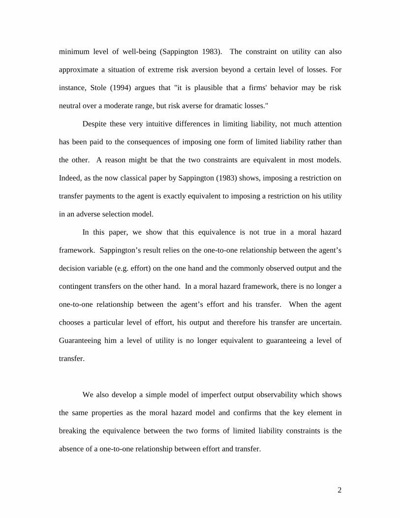
In figure 1, we illustrate the optimal level of effort in a case where r(e)=e/(1+e)

and ϕ(e)=e2/2. The graph shows that the limit on utility constraint appears to be a much

more stringent requirement leading to a much lower optimal effort.

12

Figure 1a: Optimal Effort Under Two Forms of Limited Liability

Figure 1b: Probability of Success Under Two Forms of Limited Liability

Optimal Effort

0

0.2

0.4

0.6

0.8

1

1.2

DX 1 2 3 4 5 6 7 8 9 10 11 12 13 14 15 16 17 18 19 20 21 22 23 24

XS - XF

et

eu

Probability of Succes

0.1

0.15

0.2

0.25

0.3

0.35

0.4

0.45

0.5

0.55

1 2 3 4 5 6 7 8 9 10 11 12 13 14 15 16 17 18 19 20 21 22 23 24 25

XS-XF

r(et)

r(eu)

13

We can characterize further the two resulting contracts. First note is that it is

always possible to identify two distinct levels of liability, Lt and Lu, such that the relevant

agency problems give rise to the same level of expected utility for the agent when Lt is

the relevant liability level under constraint LLt and Lu is the relevant liability level under

constraint LLu. See lemmas 1 and 2 in appendix.

We can now formulate an interesting result emerging from the optimal contract:

for a given level of expected utility of the agent, the principal will always receive a

higher expected profit by offering the agent a liability limit on transfers (LLt) rather than

one on the utility (LLu).

The following lemma is useful in demonstrating this result.

LEMMA 3 : Given E(Ut) = E(Uu), E(Πt) > E(Πu) if

[r(et)-r(eu)](XS -X F) > ϕ(et)-ϕ(eu) (5)

PROOF: See appendix.

Therefore, as long as condition (5) holds, a contract offering a limited liability of

the type LLt will yield higher profits for the principal for any given level of expected

utility for the agent than a contract offering a limited liability of the type LLu and

generating the same level of expected utility for the agent.

14

PROPOSITION 2: Optimal contracts with limited liability on transfers Pareto

dominate optimal contracts with limited liability on utility.

PROOF: See appendix.

This result follows from proposition I. As LLu generates a larger distortion in

effort, it forces the optimal contract farther away from the first best level than LLt. The

resulting additional loss in output for the principal is not compensated by the reduction in

effort cost for the agent. This is sufficient to guarantee that inequality (5) is respected.

Therefore, given lemma 3, there is an incentive compatible contract under LLt which

Pareto dominates the best incentive compatible contract under LLu.

The intuition behind proposition 2 is illustrated in figure 2. On the graph, et and

eu represent the optimal level of effort given LLt and LLu respectively.

Figure 2: Optimal effort under LL u and LL t

A

B

C

D

e

r(e)(XS)+(1-r(e))XF

ϕ(e)

et eu

15

Condition (5) requires that the segment (A-B) be larger than the segment (C-D).

The first order conditions (equation (3)) requires that eA and eB must be in the area where

the slope of the expected production [r(et)(XS-XF)] is greater than the slope of the effort

function [ϕe(et)]. Then, it is clear that (5) is true.

Proposition 2 has important consequences for the design of optimal contracts

under limited liability. Suppose a government wishes to protect a defense contractor

from bankruptcy. This could lead the government to offer a contract constrained by a

limited liability on profit (utility)(see Stole (1994) for example). For any such contract,

Proposition 2 tells us that there exists an alternative contract derived with limited liability

on transfers that guarantees both the principal and the contractor a higher level of utility.

The reason why our result differs from Sappington’s result is that, in a moral

hazard model, when the agent chooses a level of effort, he does not know which transfer

he will receive because the output is uncertain. In a standard adverse selection, the

agent’s choice variable (whether it is the effort or another variable) has a one-to-one

relationship with the output observed by the principal.

Therefore, our result would also apply to an adverse selection model as long as

the one-to-one relationship does not exist. An example would be a standard adverse

selection model with a random shock on the output. The model becomes a hybrid mix of

adverse selection and moral hazard as in Picard (1987). Another example would be a

standard adverse selection model with imperfect output observability (Lawarrée-Van

Audenrode (1996)). Such models are, however, complex and relatively uncommon in the

literature. To focus on our point while keeping the analysis simple, we present below a

16

model of imperfect output observability where the adverse selection parameter has been

removed. We show that our propositions 1 and 2 apply.

4. Limited Liability when Output is Imperfectly Observed

Consider a model where, in equilibrium, as in our moral hazard case, the agent has only

two levels of effort. He can either work hard (e=e*) or he can shirk (e=0). Imperfect

output observability means that, when he works hard, the agent could be accused of

shirking. Precisely, we assume that the agent working hard will be recognized as such

with probability r (r>1/2) and will be said to have shirked with probability (1-r).

Symmetrically, an agent shirking will be detected with probability r. The problem for the

principal will be to induce the agent to work hard while meeting its limited liability

constraint. The difference between this model and the previous one is that here the

principal’s objective function embodies the true output and not the one observed by the

principal.

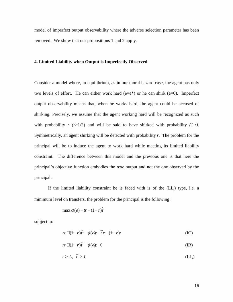
If the limited liability constraint he is faced with is of the (LLt) type, i.e. a

minimum level on transfers, the problem for the principal is the following:

trtre ~)1()( max −−−α

subject to:

rt r t e t r r t+ − − ≥ − −( )~ ( ) ~ ( )1 1ϕ (IC)

rt r t e+ − − ≥( )~ ( )1 0ϕ (IR)

t L t L≥ ≥, ~ (LLt)

17

where ~t is the transfer paid to the agent found shirking and t is the transfer paid

otherwise. Since, in this model too, t t≥ ~ , the relevant limited liability constraint is

~t L≥ . Solving the optimization problem gives the solution:

ϕ α'(.) ' (.)r

r e2 1−=

When a limited liability constraint takes the form of a constraint on the utility of

the agent (LLu), the relevant limited liability constraint will be ~ ( )t e L− ≥ϕ . Solving the

optimization problem leads to the solution:

ϕ α'(.) ' (.)3 1

2 1

r

r e

−−

=

The inspection of the two results clearly shows that the two constraints do not

lead to the same optimal level of effort. Our proposition 1 still applies. The proof is

provided in the appendix.

The proof that proposition 2 also applies is similar to the one provided for the

moral ahazard model and is available from the authors. This exercise shows that the

crucial element that differentiate Sappington’s result from our result is the presence or

not of a one-to-one relationship between effort and output.

18

Conclusions:

We have shown that under moral hazard and other frameworks where there is not

a one-to-one relationship between effort and output, modeling a limited liability

constraint as a lower limit on transfers is not equivalent to modeling it as a lower limit on

utility. Moreover, contracts with limits on transfers Pareto dominate contracts with limits

on utility. This has important implications on the design of optimal contracts. Limited

liability restrictions guaranteeing a certain level of utility to the agent are often imposed

upon the parties – like the case of bankruptcy laws for example. We have shown these

contracts to be inefficient for instance when moral hazard is present.

Note that this raises the question why the limited liability constraint was imposed

in the first place. In the introduction we mentioned Sappington’s explanation: to

guarantee a minimum level of well-being. An alternative explanation is the extreme level

of risk aversion. For instance, if the defense contactor goes bankrupt, national security

would be jeopardized. In such a case, the relevant limited liability constraint is always a

constraint on the utility.

While many legal restrictions can easily be classified as constraint on utility or

transfer, others are more difficult to categorize. Minimum wage laws, for instance, are

perfect examples of a lower limit on transfers to be paid to an agent in execution of a

work contract. Yet, by many aspects, the U.S. minimum wage law also guarantees a

certain level of utility to some workers. This is achieved by imposing minimums to

piece-rate wages and commissions, by regulating pay for overtime work as well as

working conditions, and by prohibiting the employer from imposing obligations on their

19

employees (for example forcing them to buy uniforms) which would bring their

compensation below the minimum required (Murphy, 1987).

20

Bibliography:

Brander, James and Barbara Spencer, [1989], "Moral Hazard and Limited Liability: Implications for the Theory of the Firm," International Economic Review, vol. 30, No.4, pp. 833-849.

Innes, Robert, [1990], "Limited Liability and Incentive Contracting with Ex-ante Action Choices," Journal of Economic Theory, vol. 52, pp. 45-67.

Kim Son Ku, [1997], "Limited Liability and Bonus Contracts," Journal of Economics and Management Strategy, vol.6, No.4, Winter, pp. 899-913.

Kreps, David, [1990], A Course in Microeconomic Theory, Oxford University Press.

Macho-Stadler Inés and David Perez-Castrillo, [1997], An Introduction to the Economics of Information, Oxford University Press.

Murphy, Betty, [1987], “A Guide to Wage and Hour regulation,” Corporate Practice Series, Washington, D. C.

Sappington, David, [1983], "Limited Liability Contracts between Principal and Agent," Journal of Economic Theory, vol. 29, pp. 1-21.

Schmidt, Klaus, [1997], "Managerial Incentives and Product Market Competition," Review of Economic Studies, vol.64(2), April, pp.191-213..

21

Appendix A: moral hazard model LEMMA 1: Given Lt, the following value of Lu gives the same level of expected utility to

the agent:

u

u

t

t

ee

ute

e

ttu r

ere

r

erLL ϕϕϕ ′

′−−′

′+= )(

)()(

PROOF:

At the optimum, the expected utility of the agent under LLt is given by:

E(Ut)= Lr e

ret

t

ee t

t

t+

′′ −

( )( )ϕ ϕ

while under LLu it is

E(Uu)= Lr e

ruu

ee

u

u+

′′

( )ϕ

The expected utility of the agent will be identical in both problems if

L Lr e

r

r e

ret u

u

ee

t

ee t

u

u

t

t− =

′′ −

′′ +

( ) ( )( )ϕ ϕ ϕ (A1)

LEMMA 2 : Given Lt, the following value of Lu gives the same level of expected utility to

the principal:

u

u

t

t

ee

ue

e

tutFStu r

er

r

erererXXLL ϕϕ ′

′−′

′+−−+= )()(

)]()()[(

PROOF:

At the optimum, the expected profit of the principal under LLt is given by:

t

t

ee

ttFFSt r

erLXXXer ϕ′

′−−+−=Π )(

))(()E( t (A2)

22

while under LLu it is:

u

u

ee

uuuFFSuu r

ereLXXXerE ϕϕ ′

′−−−+−=Π )(

)())(()( (A3)

Therefore the principal’s expected profit will be identical under LLt and LLu if

(A2)=(A3), i.e., if

)()()(

)]()()[( uee

ue

e

tutFStu e

r

er

r

erererXXLL

u

u

t

t

ϕϕϕ −′′

−′′

+−−+=

PROOF OF LEMMA 3:

At the optimum, the principal’s expected profit under LLt will be larger than LLu if

u

u

t

t

ee

uuuFFSue

e

ttFFSt r

ereLXXXer

r

erLXXXer ϕϕϕ ′

′−−−+−>′

′−−+− )(

)())(()(

))(( (A4)

Imposing the constraint E(Ut) = E(Uu), i.e., substituting (A1) into (A4) and rearranging

terms yields [r(et)-r(eu)](XS -X F)> ϕ(et)-ϕ(eu).

PROOF OF PROPOSITION 2:

Using a second-order Taylor expansion around et, we get:

2

)()()()(

2tu

eetuetu

eereererer

ttt

−′′+−′≈− (A5)

Similarly,

2

)()()()(

2tu

eetuetu

eeeeee

ttt

−′′+−′≈− ϕϕϕϕ (A6)

Therefore, (5) will be true if

23

2

)(

2

)()( tu

eeetu

eeeFS

eeeerrXX

tttttt

−′′+′>

−′′+′− ϕϕ (A7)

It is straightforward to verify that (A7) is true given (i) tteer ′′ < 0 and

tteeϕ ′′ > 0, (ii) (eu-et) <

0 by Proposition 1 and (iii) ter ′ >

teϕ′ from inspection of (3).

Notice that, given Lemma 2, the following “dual” relationship could also be derived:

given E(Πt) = E(Πu), E(Ut) > E(Uu).

Appendix B: imperfect output observability model

PROOF OF PROPOSITION 1: (by contradiction):

Assume eB > eA. Since ϕee> 0 and αee< 0, this implies

ϕe(eB) > ϕe(eA) (A1)

and

αe( eB) < α( eA) (A2)

Since r>1/2, we also have r

r

r

r2 1

3 1

2 1−<

−−

(A3)

Then (A1) and (A3) imply ϕ ϕe A e Ber

re

r

r( ) ( )

2 1

3 1

2 1−<

−−

(A4a)

which, given (2) and (3) implies α ϕ ϕ αe A e A e B e Be er

re

r

re( ) ( ) ( ) ( )=

−<

−−

=2 1

3 12 1

(A4b)

and this contradicts (A2).

QED.