Moral Hazard and Persistence�

Hugo HopenhaynDepartment of Economics

UCLA

Arantxa JarqueDepartment of Economics

U. of Alicante

Preliminary version (please do not quote)

Abstract

We study a multiperiod principal-agent problem with moral haz-ard in which the agent is required to exert e¤ort only in the initialperiod of the contract. The e¤ort choice of the agent in this �rst pe-riod determines the conditional distribution of output in the followingperiods. The paper characterizes the optimal compensation scheme.We �nd that the results for the static moral hazard problem extendto this setting: consumption at each point in time is ranked accordingto the likelihood ratio of the corresponding history. When output isi.i.d., as the length of the contract increases the cost of implementinge¤ort decreases, and consumption on the equilibrium path becomesless volatile. If the contract lasts for an in�nite number of periods,the cost of the principal gets arbitrarily close to that of the �rst best.Journal of Economic Literature Classi�cation Numbers: D31, D80,

D82.Key Words: mechanism design; moral hazard; persistence

�We would like to thank Árpád Ábrahám, Hector Chade, Huberto Ennis, Juan CarlosHatchondo, Leornardo Martínez, Michael Raith and seminar audiences at the Universityof Alicante, the 2006 Wegmans Conference in Rochester, the Richmond Fed, the 2006Summer Meetings of the Econometric Society in Minnesota, the 2006 Meetings of theSED in Vancouver, and the Ente Einaudi. All remaining errors are ours.

1

1 Introduction

There is a large literature on dynamic contracts that analyzes problems ofrepeated moral hazard. In the canonical model, a risk neutral principal anda risk averse agent commit to a long term contract in order to solve an incen-tive problem: each period, the unobservable e¤ort of the agent determinesthe probability distribution over the observable contemporaneous output.Current e¤ort choices a¤ect only current output, i.e., e¤ort does not havepersistent e¤ects in time. The solution to this problem speci�es the contin-gent consumption transfers that bring the agent to exert a certain level ofe¤ort, every period, at a minimum cost. There is a wide array of applica-tions of these models in macroeconomics, industrial organization, or public�nance. The lack of persistence of e¤ort is an important limitation in someof these applications, such as in the literature on incomplete insurance due toasymmetric information (see, for example, Atkeson (1991) and Phelan, 1995),CEO�s optimal compensation (Wang, 1997), optimal design of loans for en-trepreneurs (Albuquerque and Hopenhayn, 2004), or the study of optimalunemployment insurance programs (Shavell and Weiss (1979) and Hopen-hayn and Nicolini, 1997). There is a reason for this gap in the literature: itis considered a very di¢ cult problem. This paper studies a special problemof moral hazard with persistence that turns out to have an elementary solu-tion, and still allows us to learn about the implications of persistence. Thekey simpli�cation is that the agent takes only one action, at time zero, withpersistent e¤ects.The model is as follows. At the beginning of the relationship, the prin-

cipal o¤ers a contract to the agent, specifying consumption contingent ona publicly observable history of output realizations. If the agent accepts,they both commit to the contract for an exogenously speci�ed number ofperiods. The distribution over the possible output histories is determined bythe agent�s choice of e¤ort at time zero, which can take two values: low andhigh. The agent has time separable, strictly concave utility with discounting.The principal is risk neutral. For simplicity we assume the principal and theagent have the same discount factor, and the agent is not allowed to save.The problem faced by the principal is to design a contract that implementshigh e¤ort at the lowest expected discounted cost.This simple dynamic problem with persistence captures essential features

of many important long term relationships. One example is the case of in-

2

vestment in human capital1. A private �rm may o¤er wage pro�les thatencourage �rm speci�c human capital investment, or the government maywant to design the tax system in order to provide incentives for high hu-man capital accumulation. Miller (1999) originally used a variation of themodel presented here to analyze a two period problem of a car insurancecontract in which agents can a¤ect their probability of being in an accidentby exerting e¤ort when learning how to drive. In another example, Jarque(2004) evaluates the impact of compensating CEO�s with stock options whentheir actions a¤ect the output of their �rms for a number of periods. Herpaper uses our model to describe a benchmark for the optimal compensationscheme. Finally, our model has implications for the compensation of hiringcommittees of sports clubs, or editorial and record companies.With a simple relabeling of terms, our model applies to adverse selection

problems. This extends the scope of our analisys, for example, to the design ofwage pro�les when �rms face potential workers who have private informationabout their own abilities. In these situations, there is no unobservable e¤ortto be exerted at the beginning of the contract. Instead, there is asymetry ofinformation about the productivity of the agent, i.e. about the distributionof the output that he induces by working at the �rm. Assuming that anagent with high productivity has a higher outside value than one of lowproductivity, a sorting constraint takes the place of our incentive constraint:the di¤erence in expected utilities under the two possible processes for outputshould be equal to the di¤erence in outside utilities. The optimal contract issigned in equilibrium only by high productivity agents.It stems from our analysis that, in spite of its dynamic structure, our

moral hazard problem with persistence formally reduces to a static moralhazard case. In the optimal compensation scheme, all histories �regardless oftime period�are ordered by likelihood ratios, and the assigned consumptionis a monotone function of this ratio. As in the static case, compensation willbe monotone in the past realizations of output if and only if the likelihoodratios are monotonic in output. Our characterization of the optimal contracthas implications for the dynamics of consumption. The inverse of the mar-ginal utility of consumption satis�es the Rogerson condition. This impliesthat, as in most dynamic problems with asymetric information, including

1See Grochulski and Piskorski (2006) for a recent contribution to the �new public�nance�literature that explicitely models schooling e¤ort as an unobservable investmentin human capital at the beginning of life, a¤ecting future productivity of the agents.

3

standard repeated moral hazard models, the agent is savings constraint andthe evolution of his expected consumption through time depends on the con-cavity or convexity of the inverse of his marginal utility of consumption.When realizations are i.i.d. over time, our model provides some stark pre-

dictions. The contract takes a simple form: the current consumption of theagent depends only on consumption in the previous period of the contract,his tenure, and the current output realization. Longer histories contain moreinformation, so the dispersion of likelihood ratios and compensation increasesover time. Extending the number of periods reduces the cost of implement-ing high e¤ort: it reduces the need to spread consumption in earlier periods,bringing down the average variance of compensation in the contract. More-over, the cost of the contract approaches the �rst best as the number of timeperiods goes to in�nity. This result is explained by the fact that the varianceof likelihood ratios goes to in�nity with time, so asymptotically, deviationscan be statistically discriminated at no cost. The paper considers the ef-fect of reducing persistence by examining a modi�cation of the i.i.d. outputframework where the e¤ect of the initial action depreciates over time. Aspersistence decreases, the average variability of compensation increases andso does the cost of implementation.

1.1 Related Literature

There are a few papers that tackle the problem of moral hazard and per-sistence in the context of a repeated action model. Persistence changes theproblem in two dimensions: it introduces a richer information structure andit complicates the incentive problem. Information is richer because the prin-cipal observes more than one signal containing information about the samepast action. The incentive problem worsens because �joint� deviations ofe¤ort may be pro�table in the presence of persistence: when the e¤ort ofthe agent today a¤ects the conditional distribution of output tomorrow, theagent can substitute e¤ort across periods, accumulating it today in order towork less tomorrow. The changes along these two dimensions complicate boththe characterization and the numerical computation of the optimal contract.The existing literature in repeated moral hazard with persistence consists ofdi¤erent proposals of assumptions aimed at simplifying the problem along ei-ther one, or both, of those dimensions, in order to provide a characterizationof the contract with persistence.Fernandes and Phelan (2000) provided the �rst recursive treatment of

4

agency problems with e¤ort persistence. In their paper, the current e¤ortof the agent a¤ects output in the same period and in the following one.Their setup is characterized by three parameters: the number of periodsthat the e¤ect of e¤ort lasts for, the number of possible e¤ort levels, and thenumber of possible outcome realizations. All three parameters are set to twoand this makes their formulation and their computational approach feasible.The optimal contract is found by checking, one by one, all possible jointdeviations of e¤ort. The curse of dimensionality applies whenever any of thethree parameters is increased. Moreover, no results are given in their paperon how the properties of the optimal contract di¤er from the case withoutpersistence.Mukoyama and Sahin (2005) show in a two period contract that, when

the principal wants to implement high e¤ort every period and persistenceis high, it may be optimal for the principal to perfectly insure the agentin the �rst period. By restricting the number of possible e¤orts and thelength of the contract, they manage to �nd conditions on the conditionalprobabilities of output such that only a limited number of joint deviationsare relevant. Under those sets of parameters, they prove the optimalityof perfect insurance in the �rst period. In a related model, also with twopossible levels of e¤ort but for a T�period model, Kwon (2006) assumesthe probability distribution over output is concave in the sum of past e¤ort.This provides an equivalent characterization to that in Mukoyama and Sahin(2005): the optimal contract exhibits perfect insurance until period T�1; anda contingent increase in consumption in the last period of the contract. Heidenti�es this increase in consumption with a promotion, and tests the modelusing wage and promotions data from health insurance claim processors in alarge US insurance company.Jarque (2005) takes a di¤erent approach by working with a continuum of

e¤orts, but imposing two simplifying assumptions that allow for a completecharacterization of the optimal contract. First, utility is linear in e¤ort.Second, the distribution of output depends on the sum of all past discountede¤ort. This simpli�es the problem of joint deviations by making the marginaldisutility of e¤ort independent of the actual level of e¤ort chosen each period,and its marginal bene�t a function of a summary of all past histories of e¤ort.Under these assumptions, consumption in the optimal contract exhibits thesame properties as consumption in a repeated moral hazard problem withoutpersistence.All these four papers simplify the joint deviations problem, either by lim-

5

iting the possible e¤orts, the span of persistence in time, or by imposingrestrictions directly on how the conditional probabilities depend on e¤ort.With these assumptions, these models are as well imposing restrictions onthe information structure: their assumptions imply limits to the amount ofinformation about past e¤ort that is embedded in future realizations of out-put. The model we propose in this paper complements the existing literatureby exploring the implications of the richest possible information structure un-der persistence. We maximize the information about past e¤ort contained ineach output realization, since the conditional distribution of all future out-put is determined by the initial e¤ort. However, we completely eliminatethe possibility of joint deviations, and its interaction with the informationstructure, since the agent only exerts e¤ort once. This simpli�cation allowsus to fully characterize the contract.The paper is organized as follows. A characterization of the optimal

contract is given for the general model in the next section. Results andnumerical examples for the i.i.d. case are discussed in section 3, and section 4includes the asymptotic result. In section 5 we present the case of decreasingpersistence.

2 The Model

The relationship between the principal and the agent lasts for T periods,where T is �nite.2 There is the same �nite set of possible outcomes eachperiod, fyigni=1 ; with yi < yi+1 for all i = 1; : : : ; n. Let Y t denote the setof histories of outcome realizations up to time t; with typical element yt =fy1;y2; :::; ytg : This history of outcomes is assumed to be common knowledge.The agent�s e¤ort can take two possible values, e 2 feL; eHg :3 A contractprescribes an e¤ort to the agent at time 1; as well as a transfer ct fromthe principal to the agent, contingent on the history of outcomes up to the

2The solution to the problem presented here is not well de�ned when T = 1. Thecase of in�nite T is dealt with in the last section of the paper, where an asymptoticapproximation result is presented.

3As it becomes clear in the core of the paper, the results presented here generalizeto the case of multiple e¤ort levels as much as those of a static moral hazard problem.That is, it may be that some of the levels are not implementable, and for a continuum ofe¤orts we would need to rely on the validity of the �rst order approach to �nd the optimalcontract.

6

present time: ct : Y t ! R+; for t = 1; 2; :::; T .4 Each period, the probabilityof a given history of outcomes is conditional on the e¤ort level chosen atthe beginning of the �rst period: Pr (ytje) : With this speci�cation, we allowthe distribution of the period outcome to change over time, including thepossibility of dependent realizations across periods (i.e., persistent output).We assume Pr (ytje) strictly positive for all possible histories and for bothlevels of e¤ort. Both the agent and the principal discount cost and utility atthe same rate �. Commitment to the contract is assumed on both parts.As in most principal�agent models, the objective of the principal is to

choose the level of e¤ort and the contingent transfers that maximize herexpected pro�t, i.e., the di¤erence between the expected stream of outputand the contingent transfers to the agent. In the context of a static moralhazard problem, Grossman and Hart [5] showed in their seminal paper thatthis problem can be solved in two steps. The same procedure applies in ourdynamic setting: �rst, for any possible e¤ort level, choose the sequence ofcontingent transfers that implement that e¤ort in the cheapest way. Thecost of implementing e¤ort e in a T period contract is just the expecteddiscounted stream of consumption to be provided to the agent:

K (T; e) =TXt=1

Xyt

�t�1�c�yt�Pr�ytje

�:

Second, choose among the possible e¤orts the one that gives the biggestdi¤erence between expected output and cost of implementation. Note that,as it is the case in static models, implementing the lowest possible e¤ort istrivial: it entails providing the agent with a constant wage each period suchthat he gets as much utility from being in the contract as he could get workingelsewhere. Since the interesting problem is the one of implementing eH ; weassume throughout the paper that parameters are such that the second stepof the general problem always �nds it pro�table to implement eH ; and wedrop the dependence of total cost on the e¤ort level: K = K (eH) : We alsoassume unlimited resources on the part of the principal, so we do not need tocarry his balances throughout the contract. A contract is then simply statedas a sequence of contingent consumptions, fc (yt)gTt=1.

4Even though unlimited punishments are needed for the asymptotic results of the paper,the restriction on consumption is without loss of generality; we only need utility to beunbounded below.

7

The expected utility that the agent gets from a given contract, contingenton his choice of e¤ort, is

U�e;�c�yt�T

t=1

�=

TXt=1

Xyt

�t�1u�c�yt��Pr�ytje

�� e;

where e denotes both the choice of e¤ort and the disutility implied by it.Letting U denote the agent�s outside utility, the Participation Constraint(PC) reads:

U � U�eH ;

�c�yt�T

t=1

�; (PC)

When e¤ort is observable, the optimal contract (sometimes referred to as theFirst Best) is the solution to the following cost minimization problem:

minfc(yt)gTt=1

TXt=1

Xyt

�t�1�c�yt�Pr�ytjeH

�s:t: PC

It is easy to show that the First Best calls for perfect insurance of the agent.When e¤ort is observable, a constant wage minimizes the cost of deliveringthe outside utility level. The constant wage c� in the First Best satis�es:

U + eH =1� �T

1� � u (c�) :

Later in the paper we use the cost of the �rst best scheme, K� � 1��T1�� c

�

as a benchmark for evaluation of the severity of the incentive problem whene¤ort is not observable.Given the moral hazard problem due to the unobservability of e¤ort, the

standard Incentive Compatibility (IC) condition further constrains the choiceof the contract:

U�eH ;

�c�yt�T

t=1

�� U

�eL;�c�yt�T

t=1

�: (IC)

In words, the expected utility of the agent when choosing the high level ofe¤ort should be at least as high as the one from choosing the low e¤ort.In order to satisfy this constraint, the di¤erence in costs of e¤ort shouldbe compensated by assigning higher consumption to histories that are more

8

likely under the required action than under the deviation. Formally, theoptimal contract (often referred to as the Second Best) is the solution to thefollowing cost minimization problem:

minfc(yt)gTt=1

TXt=1

Xyt

�t�1�c�yt�Pr�ytjeH

�s:t: PC and IC

The optimal contract can be characterized by looking at the �rst orderconditions of this problem. As in the static moral hazard case, the LikelihoodRatio of a history yt; denoted as LR (yt) ; can be de�ned as the ratio of theprobability of observing yt under a deviation, to the probability under therecommended level of e¤ort:

LR�yt�� Pr (ytjeL)Pr (ytjeH)

:

Proposition 1 The optimal sequence fc� (y� )gT�=1 of contingent consump-tion in the Second Best contract is ranked according to the likelihood ratiosof the histories of output realizations, i.e., for any two histories yt and eyt0 of(possibly) di¤erent lengths t and t0;

c�yt�> c

�eyt0�, LR�yt�< LR

�eyt0�Proof. Since utility is separable in consumption and e¤ort, both the PCand the IC are binding. From the FOC�s,�

c�yt��:

1

u0 (c (yt))= �+ �

�1� LR

�yt��

8yt; (1)

where � > 0 and � > 0 are the multipliers associated with the PC and theIC respectively. Since u0 (�) is decreasing, the result follows from the aboveset of equations.This characterization implies that, in spite of its dynamic structure, this

problem can be reduced to a standard static moral hazard case. The agentchooses e¤ort only once, at the beginning of the relationship. This makesthe principal indi¤erent between minimizing the total cost of the contract orthe corresponding average per period cost. Once this alternative speci�ca-tion is considered, it becomes apparent that there is a one to one mapping

9

between the average per period cost minimization problem and a static costminimization problem.The intuition for this result is the following. The information structure

for the standard moral hazard case is given by a set of states and proba-bility distributions over these states, conditional on the actions. The agentmaximizes expected utility, which is a convex combination of the utility as-sociated to each state with the corresponding probabilities. Let the states inthe dynamic case be the set of all histories (all possible nodes in the tree),i.e. [Tt=1Y t: To each state and for each possible e¤ort choice, assign a weightequal to the original probability of the history, adjusted by the correspondingdiscount factor. All probabilities can be normalized, so they add up to one:to history yt corresponds a weight equal to

1� �1� �T

�t�1 Pr�ytje

�:

This is the weight assigned to any history in the average per period costminimization problem. The expected discounted utility of any contingentconsumption plan reduces to a convex combination of the utilities in each ofthese states, with these adjusted weights. The intuition for the propositionabove becomes clear. The optimal compensation scheme is derived as in thestatic moral hazard problem: all histories �regardless of time period� areordered by likelihood ratios, and the assigned consumption is a monotonefunction of this ratio. As in the static problem, the contract tries to balanceinsurance and incentives. To achieve this optimally, punishments (lower con-sumption levels) are assigned to histories of outcomes that are more likelyunder a deviation than under the recommended e¤ort, i.e., to those that havea high likelihood ratio.Consumption in the optimal contract depends on the whole history of

output realizations available, and it is, typically, a non linear function of totaloutput. We can, however, establish conditions for some form of monotonicityof consumption in output, paralleling standard results in the moral hazardliterature. Throughout the paper, we use LR (yt) to denote the likelihoodratio of an individual realization of output at time t:

LR (yt) =Pr (ytjeL; yt�1)Pr (ytjeH ; yt�1)

:

De�nition 2 The Monotone Likelihood Ratio Property holds at the

10

individual output level in period t if and only if, for any yt�1; the individualoutput likelihood ratio at t, LR (yt) ; decreases monotonically with yt:

Proposition 3 For any given �nite history yt�1; c (yt�1; yi) > c (yt�1; yj) ;for all i > j; if and only if the MLRP holds at the individual output level inperiod t:

Proof. From the MLRP at the individual output level in period t;

LR�yt�1; yi

�= LR

�yt�1

�LR (yi) < LR

�yt�1

�LR (yj) = LR

�yt�1; yj

�8i > j:

The ranking of consumptions follows directly from the FOC�s stated in Eq.1.In our dynamic setup, the MLRP for individual outcomes is satis�ed by

a small set of processes for output. We can think of a weaker restriction thatstill assures some form of monotonicity. Consider the following (incomplete)order relation for histories of the same length:

De�nition 4 A history yt = (y1; y2; : : : ; yt) is a better history than eyt =(ey1; ey2; : : : ; eyt) if and only if y� � ey� for all � = 1; : : : ; t, with strict inequalityfor at east one � .

We can state a monotonicity property of Likelihood Ratios, but at thelevel of histories as opposed to individual outputs:

De�nition 5 The Monotone Likelihood Ratio Property holds at thehistory level in period t if and only if, for any two histories yt;and eyt suchthat yt is better than eyt; the history likelihood ratio of yt is smaller than thatof eyt, that is,

LR�yt�< LR

�eyt� :Note that since the likelihood ratio of a history is the product of the

individual output histories, if MLRP holds at the individual outcome levelfor all periods up to t; it also holds at the history level in period t:

Proposition 6 For any two histories yt and eyt such that yt is better thaneyt; the optimal contract implies c (yt) > c (eyt) if and only if the MLRP holdsat the history level in period t:

11

Proof. Straight from eq. 1, MLRP at the history level implies the statedranking of consumption.In spite of the parallel that we established with the solution to a sta-

tic moral hazard problem, some of the features that we observe in dynamicasymmetric information models are present also in our problem with persis-tence. The FOC�s of the problem described in equation 1 can be combined toget the condition on the inverse of the marginal utility derived by Rogerson[17] in the context of a two period repeated moral hazard problem:

1

u0 (c (yt))=Xyt+1

1

u0 (c (yt; yt+1))Pr�yt+1jeH ; yt

�: (2)

This equality shows that our problem with persistence exhibits the standarddynamic trade�o¤ between incentives and consumption smoothing. As inRogerson [17], this property implies that the agent, if allowed, would like tosave part of his wage every period in order to smooth his consumption overtime. Other properties discussed by Rogerson are also true in this setup, asindicated in the next proposition.

Proposition 7 In the Second Best contract, the expected wage decreases withtime whenever 1

u0(�) is convex, increases if it is concave, and is constant when-ever utility is logarithmic. (Rogerson)

Proof. As in the dynamic moral hazard problem studied by Rogerson, (2)holds. Take the case of 1

u0(c) being concave. By Jensen�s inequality,

1

u0 (c (yt))>

1

u0 (E [c (yt; yt+1)])

u0�E�c�yt; yt+1

���> u0

�c�yt��:

Since utility is concave,

c�yt�< E

�c�yt; yt+1

��:

A similar argument applies for the other two cases.We now turn to the special case in which output follows an i.i.d. process,

and further characterize the contract. We show that persistence has verydi¤erent long run implications for consumption than those found in the stan-dard dynamic contract literature.

12

3 Outcomes Independently and Identically Dis-tributed

In this section, we study a particular speci�cation of the probability distrib-ution of outcomes: an i.i.d. process. We have

Pr�ytje; yt�1

�= Pr (ytje) 8yt; t = 1; :::; T:

This assumption puts additional structure on the probability distribution ofhistories, and allows for the optimal contract to be further characterized.Suppose each period there are only two possible outcomes, fyL; yHg : To

simplify notation, let

Pr (yH jeH) = �

Pr (yLjeH) = 1� �:

If the low e¤ort is chosen instead,

Pr (yH jeL) = b�Pr (yLjeL) = 1� b�;

with � > b�:Note that

LR(yH) =b��< 1

and

LR(yL) =1� b�1� � > 1:

For any history yt, the fraction of high realizations is a su¢ cient statistic forthe history�s probability. Denote the number of high realizations containedin a given history as x (yt) : The likelihood ratio of the history can be writtenas

LR�yt�=

�b��

�x(yt)�1� b�1� �

�t�x(yt)and the �rst order conditions for a history of length t read:�c�yt�1; yH

��:

1

u0 (c (yt�1; yH))= �+ �

�1� LR

�yt�1

� b��

��c�yt�1; yL

��:

1

u0 (c (yt�1; yL))= �+ �

�1� LR

�yt�1

� 1� b�1� �

�8yt�1:

13

We can easily see that in the two outcome setup the MLRP holds trivially,both at the individual outcome level and for histories. Hence, we can simplifythe general results on monotonicity of consumption given in the previoussection:

Corollary 8 Assume output can only take two values, fyL; yHg ; and it isi.i.d. over time. Given any history yt of any �nite length t, c (yt; yH) >c (yt; yL). In other words, the consumption of the agent increases when anew high realization is observed.

When output is i.i.d., the order relation introduced in De�nition4 is com-plete. Using the new notation, a history is better than any other history ofthe same length if and only if it has a higher x (�) :

Corollary 9 For any two histories of the same length yt and eyt; c (yt) �c (eyt) if and only if x (yt) � x (eyt) ; regardless of the sequence in which therealizations occurred in each of the histories.

In other words, there is perfect substitutability of output realizationsacross time. This implies, in fact, that x (yt) contains all the informationabout history yt that is used in the optimal contract. Faced with a currentoutput realization yt following a given history yt�1, we only need to knowx (yt�1) to determine current compensation. Simply put, the consumptionreceived by the agent in the previous period, together with his tenure in thecontract are su¢ cient to determine his current consumption.Under the i.i.d. assumption, we can study the evolution of the values

of the likelihood ratios at each period. We can translate this into formalproperties of the support of the contract, that is, the evolution of the possiblevalues of consumption through time. Denote yt the history at t with all highoutcomes, that is, the history of length t that satis�es x (yt) = t: Similarly,yt denotes the one with all low outcomes, with x

�yt�= 0: The following

simple proposition says that the range of variation in consumption within acertain period is larger in the latter periods of the contract and the di¤erencebetween the highest and the lowest consumption within a period, denoted bydt; increases with time.

Proposition 10 As t increases, c (yt) increases and c�yt�decreases. Hence,

as t increases, dt = c (yt)� c�yt�increases.

14

Proof. In the i.i.d. case, for a length t, the lowest likelihood ratio is that ofthe history with t high realizations of output:

LR�yt�=b�t�t:

For the highest, instead, it is

LR�yt

�=(1� b�)t(1� �)t

:

Given that b��< 1 and (1�b�)

(1��) > 1;

LR�yt�> LR

�yt+1

�;

LR�yt

�< LR

�yt+1

�:

The result follows from the First Order Conditions.We can characterize the distribution of the likelihood ratios over time

and use its moments to study stochastic properties of consumption over timein the optimal contract. To each history yt corresponds a likelihood ratioLR (yt) : The probability of observing that particular likelihood ratio is theprobability of history yt: Under high e¤ort choice, for example,

Pr�LR

�yt�jeH�=

�x (yt)t

��x(y

t) (1� �)1�x(yt) :

We can calculate the expectation and the variance of the likelihood ratios ateach t: The expectation in equilibrium is constant over time, and equal toone:

E�LR

�yt�jeH�=Xyt

Pr�ytjeH

� Pr (ytjeL)Pr (ytjeH)

=Xyt

Pr�ytjeL

�= 1 8t:

The variance of the likelihood ratios at time t is more easily expressed interms of E [LR (yt) jeL] ; the expectation o¤ the equilibrium path. This, inturn, can be written in terms of the expectation at t = 1: We introduce thefollowing notation:

bE � E �LR �y1� jeL� = b�b��+ (1� b�) (1� b�)

(1� �) :

15

Any values of � and b� that satisfy our initial assumption of � > b� implybE > 1: It is easy to check thatE�LR

�yt�jeL�= bEt:

After some algebra, we get the following expression for the variance of thelikelihood ratios under high e¤ort, which we denote by vt :

vt � V ar�LR

�yt�jeH�= bEt � 1:

The variance of the likelihood ratios is a measure of informativeness of theinformation structure that the principal is facing. More variance of the like-lihood ratios, however, translates into more extreme values for consumption,as we have seen in the last proposition. We need to analyze the solutionto the optimal contract to quantify how much of the variation in likelihoodratios optimally translates into variation of consumption in equilibrium, andhow this a¤ects the cost of the contract.As we have already mentioned for the case of more general processes

for output, the inverse of the marginal utility of consumption satis�es themartingale property. From the same �rst order conditions of the problem(Eq.1), in the i.i.d. case, we can characterize the evolution of the variance ofthe inverse of the marginal utility of consumption. Although this is not, ingeneral, a direct measure of the evolution of consumption, it is closely relatedto it, and provides us with a measure of risk smoothing across periods in theoptimal contract.

Proposition 11 The variance of 1u0(c(yt)) increases with t: The one�period

increase in the variance also increases with t:

Proof. By the �rst order conditions,

1

u0 (c (yt))= �+ �

�1� LR

�yt��

8t

so we have that

E

�1

u0 (c (yt))jeH�= �:

and

V ar

�1

u0 (c (yt))jeH�

= �2vt

= �2� bEt � 1� ;

16

which is obviously increasing in t: For any two periods t and t + 1; for t =1; : : : ; T � 1; the one�period increase in the variance equals

V ar

�1

u0 (c (yt+1))jeH�� V ar

�1

u0 (c (yt))jeH�

= �2� bEt+1 � bEt�

= �2 bEt � bE � 1� :This expression is positive, since bE > 1: If we take the di¤erence betweentwo adjacent increments, we get an expression that is always positive:

�2 bEt+1 � bE � 1�� �2 bEt � bE � 1� = �2 bEt � bE � 1�2 ;establishing the second part of the proposition.We postpone the discussion of this proposition to state two corollaries

that rely on the same intuition. The �rst one applies to the special casein which the agent has logarithmic utility. Since u0 (c) = 1

c; in this case

the above proposition applies directly to the variance of consumption in theoptimal contract:

Corollary 12 When the agent has u (c) = ln (c), the variance of c (yt) in-creases with t: The one�period increase in this variance also increases witht:

There is a second functional form for utility that provides, not only anintuitive measure for the optimal way of smoothing incentives over time,but also close form solutions for the optimal contract: u (c) = 2

pc, which

corresponds to a CRRA utility function with coe¢ cient of risk aversion equalto 1

2:

Corollary 13 When the agent has u (c) = 2pc, the variance of u (c (yt))

increases with t: The one�period increase in this variance also increases witht:

Proof. Since 1u0(c) =

pc; we have that

V ar�u�c�yt��jeH�= V ar

h2pc (yt)jeH

i= 4V ar

�1

u0 (c)jeH�:

17

By Prop.11, we know that V arh

1u0(c) jeH

iincreases with t: The second part

of the corollary follows in the same way.As we discussed in the light of Prop.1, the contract optimally places incen-

tives in the later periods of the contract, where information is more precise.The higher precision of the information is captured by the increasing vari-ance of the likelihood ratios towards the later periods of the contract. This,in turn, implies higher variation in consumption in later periods. In otherwords, the optimal contract provides higher insurance and less incentivesin the initial periods, and decreases insurance in favor of incentives lateron, when punishments can be placed more e¢ ciently in light of the richerinformation.

u (c) = ln (c) u (c) = 2pc

(c� = 1:3225) (c� = 9:9742)K(4)K� = 1:32

K(4)K� = 1:14

E[ct]c�

�tE[ct]

dtct

t = 1 1:32 0:30 0:8t = 2 1:32 0:44 2:1t = 3 1:32 0:54 5:3t = 4 1:32 0:63 132:1

E[ct]c�

�tE[ct]

dtct

t = 1 1:05 0:49 1:6t = 2 1:11 0:63 4:7t = 3 1:17 0:70 12:9t = 4 1:24 0:73 58:1

Table 1. Numerical examples

In Table 1 we report values for two examples, with the two functionalforms of our corollaries, as an illustration of the results.5 Both contracts lastfour periods and share all the parameters. In the �rst column, as predictedby Prop.7, we observe that expected consumption is constant across periodsfor the logarithmic utility, while it is increasing for the square root case,which has the inverse of the marginal utility concave in consumption. In the

5Parameters of the example: T = 4, � = :95, U= 2, eH = :3; eL = 0; � = :3; b� = :2:18

second column we report the standard deviation of consumption (we divide itby the expected consumption in the period so that numbers are comparableacross periods and utility speci�cations). As predicted by Corollaries 12 and13, the numbers increase with t:6 For the logarithmic case, for example, inthe �rst period of the contract the scaled standard deviation of consumptionis 0.3. At the fourth period of the contract, the value increases to 0.63. Weobserve the same trend for the square root utility. The third column reportsthe di¤erence between the highest and the lowest consumption levels in agiven period, dt; relative to the lowest consumption:

dtct=ct � ctct

:

This normalization captures the fact that, since utility is concave, the samedt represents more variation in utility when the levels of consumption arelower. Consistently with the result in Prop.10, dt

ctincreases with t: For the

logarithmic case, in the �rst period the scaled di¤erence of consumption is0.8, and it increases to 132.1 by the fourth period. We observe the sametrend for the square root utility.We can as well do comparative statics with respect to the individual

outcome probabilities, � and b�: We can easily characterize how changes inthe values of these probabilities a¤ect vt. Morover, the variance of the inverseof the marginal utility of consumption at time t is inversely proportional tothe variance of the likelihood ratios, vt:We can establish the following results:

Lemma 14 For a �xed �; when b� increases (decreases), the variance of1

u0(c(yt)) increases less (more) over time

Proof. When b� increases, bE decreases, and hence vt and the increase ratein the variance of the inverse of the marginal utility are both smaller.

Corollary 15 For a �xed �; when b� increases (decreases), (a) if the agenthas u (c) = ln (c) ; the variance of consumption increases less (more) overtime, (b) if the agent has u (c) = 2

pc; the variance of utility increases less

(more) over time.

6Although our result for the square root utility implies increasing variance of utilityvalues, we see in all of our numerical examples that the same holds for the variance ofconsumption.

19

A smaller di¤erence between � and b� represents a more severe incentiveproblem. Our previous Lemma can be restated as saying that a more severeincentive problem translates into a provision of incentives that is more uni-formly spread throughout the duration of the contract. Since we are keeping� �xed, each history is reached with the same probability as it was before thechange in b�: The distributions of output under high and low e¤ort becomemore di¢ cult to discriminate statistically, even as we get to later periods ofthe contract. There is less bene�t in waiting to provide incentives, so thespread of consumption is more even across periods. Wether the average vari-ance of utility will decrease or increase with changes in b� involves quantifyingthe implied changes in the multipliers. We can do that for the square rootutility function.

Proposition 16 Consider the case in which the agent has utility functionu (c) = 2

pc: For a �xed �; when b� increases (decreases) the average variance

of utility across periods increases (decreases) and the cost of the contractincreases (decreases).

Proof. This functional form also allows us to �nd explicit solutions for themultipliers, using the FOC�s and the constraints of the problem:

� =(U + eH)

2and

� =eH=2

�vT;

where �vT denotes the average across periods of the variances of the likelihoodratios, in a T period contract:

�vT �PT

t=1 �t�1vt

1��T1��

:

By the results above we have

V ar�u�c�yt��jeH�= 4�2vt:

We can substitute the expression for � to write the variance of utility at eachperiod as a function of vt and �vT only:

V ar�u�c�yt��jeH�= 4

�eH=2

�vT

�2vt

= e2Hvt�v2T:

20

Taking the average across periods, we havePTt=1 �

t�1V ar [u (c (yt)) jeH ]1��T1��

=e2H�vT:

When b� increases, bE decreases, and hence vt decreases in each period, making�vT smaller. This makes the average variance of utility higher. The secondpart of the proposition states that the expected cost of the contract increaseswith an increase in b�. The expression for consumption is:

c�yt�=��+ �

�1� LR

�yt���2

:

We can write expected consumption at each t as a function of E [utjeH ]2 andV ar [utjeH ] :

E [ctjeH ] =1

4

�E [utjeH ]2 + V ar [utjeH ]

�=1

4

�(U + e)2 + e2H

vt�v2T

�:

The average per period cost of the contract is then easily written as:

k (T ) =1

4

�1� �T

1� � (U + e)2 +e2

�vT

�:

Since �vT decreases with b�; we have that k (T ) is bigger for higher b�; and sois K (T ).This result, combined with Corollary15, provides us with a clear picture

of the di¤erences we should observe across contracts with di¤erent levels ofincentive problems, as represented by the di¤erence ��b�: In worse situations,when ��b� is smaller, the cost of the contract is higher, since average varianceof compensation is higher, and variation of consumption is more even acrossperiods. Problems with big ��b�; instead, concentrate incentives only in lesslikely histories towards the end of the contract, implying a sharper increaseof the variance in time. We have shown, however, that average variance ofcompensation is lower, and hence the cost of the contract is also lower.The higher quality of information implied by a higher ��b� translates into

a lower �: The multiplier � determines howmuch of the variation in likelihoodratios translates into variation in compensation: for a given fvtgTt=1, when� � b� increases � decreases and compensation is less variable. However,when �� b� increases, vt increases as well in every period, the increase being

21

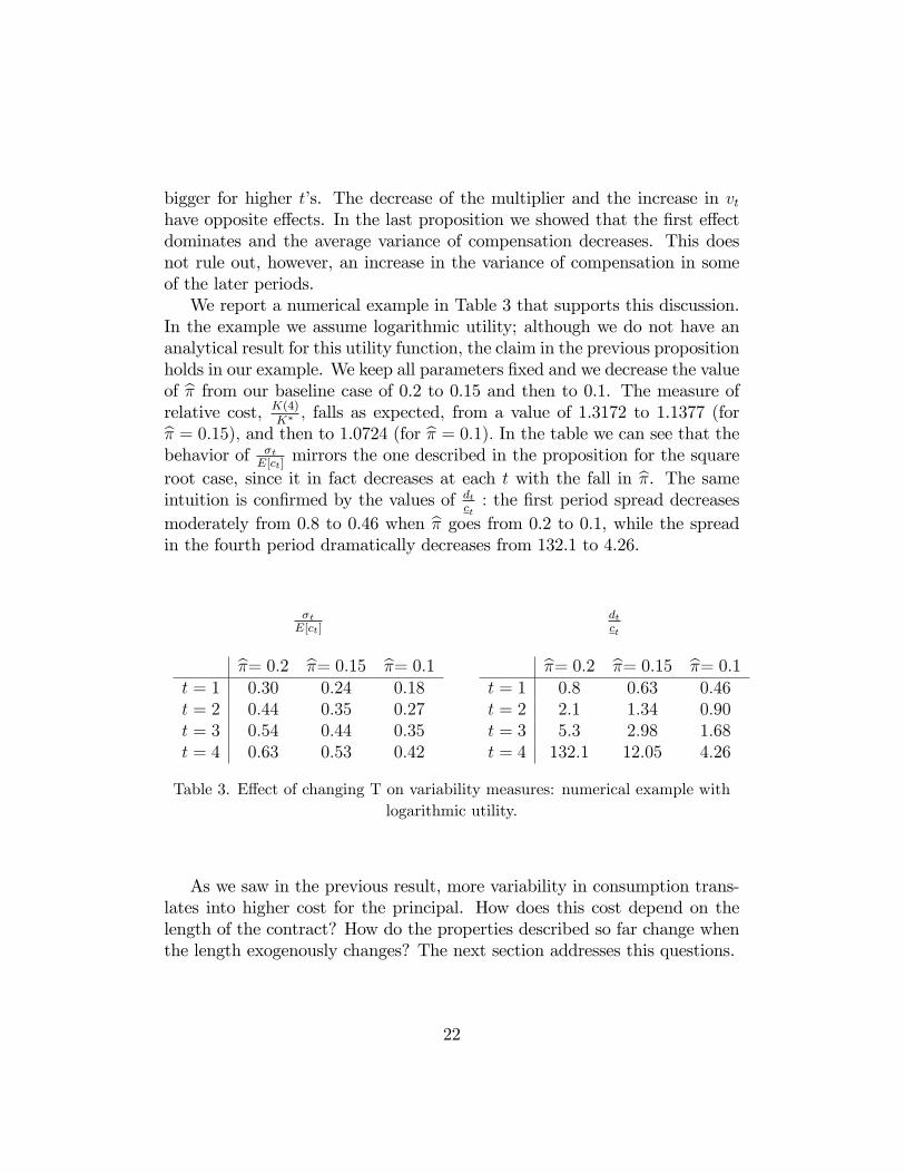
bigger for higher t�s. The decrease of the multiplier and the increase in vthave opposite e¤ects. In the last proposition we showed that the �rst e¤ectdominates and the average variance of compensation decreases. This doesnot rule out, however, an increase in the variance of compensation in someof the later periods.We report a numerical example in Table 3 that supports this discussion.

In the example we assume logarithmic utility; although we do not have ananalytical result for this utility function, the claim in the previous propositionholds in our example. We keep all parameters �xed and we decrease the valueof b� from our baseline case of 0.2 to 0.15 and then to 0.1. The measure ofrelative cost, K(4)

K� ; falls as expected, from a value of 1.3172 to 1.1377 (forb� = 0:15); and then to 1.0724 (for b� = 0:1): In the table we can see that thebehavior of �t

E[ct]mirrors the one described in the proposition for the square

root case, since it in fact decreases at each t with the fall in b�. The sameintuition is con�rmed by the values of dt

ct: the �rst period spread decreases

moderately from 0.8 to 0.46 when b� goes from 0.2 to 0.1, while the spreadin the fourth period dramatically decreases from 132.1 to 4.26.

�tE[ct]

dtct

b�= 0:2 b�= 0:15 b�= 0:1t = 1 0:30 0:24 0:18t = 2 0:44 0:35 0:27t = 3 0:54 0:44 0:35t = 4 0:63 0:53 0:42

b�= 0:2 b�= 0:15 b�= 0:1t = 1 0:8 0:63 0:46t = 2 2:1 1:34 0:90t = 3 5:3 2:98 1:68t = 4 132:1 12:05 4:26

Table 3. E¤ect of changing T on variability measures: numerical example withlogarithmic utility.

As we saw in the previous result, more variability in consumption trans-lates into higher cost for the principal. How does this cost depend on thelength of the contract? How do the properties described so far change whenthe length exogenously changes? The next section addresses this questions.

22

4 Changes in the Length of the Contract

When output is assumed to be i.i.d., longer contracts have a richer informa-tion structure. We now proceed to show that a richer information structureallows the implementation of high e¤ort at a lower average per period cost.We make explicit this point in the next two propositions. We also present,for the square root utility function, results on the e¤ect of contract length onthe measures of variability of compensation, and we complement the analysiswith some numerical examples.While doing comparative statics on the number of periods in the contract,

we wish to abstract from the fact that it is usually cheaper to provide a givenlevel of utility in several periods than in one period, simply because theagent�s utility function is concave. As T grows, we make the agent�s outsideutility depend on the length of the contract, interpreting U as a one�periodopportunity cost. To simplify notation, denote

�(T ) � 1� �T

1� � :

Abusing notation, we can write the outside utility of a T�long contract interms of U simply as

U (T ) = � (T )U:

We need to change as well the speci�cation of the e¤ort cost, so that theincentive constraint does not become looser when increasing the contractlength T: The same normalization used for outside utility is used for thedisutility of e¤ort, which now depends on T :7

e (T ) = � (T ) e for e = feL; eHg :

We de�ne the average per period cost of the contract as the k (T ) that sat-is�es:

K (T ) =TXt=1

�t�1k (T ) ;

7With this normalization, we are in fact changing more than T when we do the com-parative statics. However, for discount factor � not too low, if we were to hold U and eHconstant when increasing T our results on the decrease of cost would only be reinforced.

23

so we can simply write it as

k (T ) =1

� (T )K (T ) :

Proposition 17 Longer contracts have a lower average per period cost.

Proof. Consider the problem of �nding the optimal dynamic contract for agiven length T: Let n (t) denote the number of time�t histories and chose anarbitrary ordering so that ytj; with j ranging from 1 to n (t) ; denotes a typicalt�period history (for the two outcome case we consider here, n (t) = 2t). Eachhistory happens with probability Pr

�ytjjeH

�or Pr

�ytjjeL

�; conditional on the

e¤ort chosen. We now de�ne a static moral hazard problem that is identicalto this dynamic one. Let the state space be the whole set of possible histories,of any length: S (T ) = [Tt=1

nyt1; :::; y

tn(t)

o: For each t = 1; : : : ; T; de�ne the

following probabilities

qTjt =�t Pr

�ytjjeH

��(T )

; for j = 1; :::; t+ 1:

Each original probability is adjusted so that we haveP

jt qTjt = 1: Similarly

de�ne probabilities bqTjt by adjusting the distribution Pr �ytjjeL� : NormalizingU (T ) ; eH (T ) ; and eL (T ) ; the original problem can be rewritten as:

minc(ytj)

Xj;t

qTjtc�ytj�

subject to: Xj;t

u�c�ytj��qTjt �

eH (T )

� (T )� U (T )

� (T )Xj;t

u�c�ytj��(qTjt � bqTjt) �

�eH (T )

� (T )� eL (T )� (T )

�:

This corresponds to the problem of minimizing average per period cost ofthe contract, subject to the original constraints. Its solution coincides withthat of our original dynamic problem, since it constitutes a simple monotonic

24

transformation. Given the adjusted weights, it is easy to see that its totalcost is equal to the average per period cost of the original problem:

minc(ytj)

Xj;t

qTjtc�ytj�=

1

� (T )minc(ytj)

Xj;t

Pr�ytjjeH

�c�ytj�=

1

� (T )K (T ) = k (T ) :

By simple inspection it is apparent that the above problem has the structureof a static contract. Now suppose we decrease the number of time periodsto T � 1: De�ne a static problem by using the same state space as above,S (T ) ; but assigning zero probability to those states that correspond to T�period histories, i.e., yTj for j = 1; : : : ; n (T ). To all other histories, assignprobabilities qT�1jt and bqT�1jt as done above (note that we need to use�(T � 1)instead of �(T )): The corresponding T � 1 period moral hazard problem isequivalent to the above, replacing �(T � 1) for �(T ) : (It follows from ourde�nitions that e (T ) =�(T ) = e (T � 1) =�(T � 1) and the same holds forU(T ).) It is easy to show that the information structure

�qTjt; bqTjt� is su¢ cient

for�qT�1jt ; bqT�1jt

�(in the sense of Blackwell), so by Grossman and Hart [5],

Prop. 13, it follows that:

k (T ) � k (T � 1)

which completes the proof.The intuition for this result hinges on the better quality of the signal struc-

ture of the problem when the contract is longer. As already established byHolmström [7], any informative signal is valuable. Under the assumption ofan i.i.d. process for output determined by the initial e¤ort, a longer contracttranslates into a greater number of informative signals. When more peri-ods are available, information quality increases and incentives can be givenmore e¢ ciently: the wage scheme calls for less variation in the early periods,since punishments in later periods are exercised with lower probability onthe equilibrium path.When the agent has u (c) = 2

pc; we can explicitly characterize the change

in average per period cost as a function of the length of the contract. Weestablish the following result.

Proposition 18 When the agent has utility function u (c) = 2pc; longer

contracts have strictly smaller average per period cost.

25

Proof. The expression for expected consumption at each t is:

c�yt�=

��+ �

�1� Pr (ytjeL)

Pr (ytjeH)

��2:

With this we can write expected consumption at each t as:

ET [ctjeH ] =1

4

�E [u (ct) jeH ]2 + V ar [u (ct) jeH ]

�:

The average per period cost of the contract is then easily written as:

k (T ) =1

4

�E [u (ct) jeH ]2 +

e2

�vT

�=1

4

�(U + e)2 +

e2

�vT

�;

where �vT is the average across periods of the variance of the likelihood ratios,vt: It is easy to see that k (T ) is smaller for higher T; since �vT increases withT .As we discussed in the previous section, the cost of the contract for this

speci�cation of the utility function is negatively related with the averagevariance of the likelihood ratios. When evaluating the e¤ects of a changein (� � b�) ; we used the variation in �vT to establish implications for costand average variance of compensation. When doing comparative statics withrespect to T; we can characterize the changes in the variance of compensationof each individual period. Let V arT [u (c (yt)) jeH ] denote the variance ofutility in period t when the contract lasts for T periods.

Proposition 19 When the agent has utility u = 2pc; the variance of con-

sumption in a given period is lower when the contract is longer, i.e.,

V arT�u�c�yt��jeH�< V arT�1

�u�c�yt��jeH�for t < T; 8T:

Proof. We can express variance of utility as a function of �vT using thesolution for � :

V ar�u�c�yt��jeH�= e2H

vt�v2T:

When we go from a T � 1�period contract to a T�period contract each vtremains the same. The average across periods, �vT increases, since vT > vtfor each t < T .

26

u = 2pc u = ln (c)

T = 1 1:36 2:73T = 2 1:24 1:73T = 3 1:17 1:45T = 4 1:14 1:32

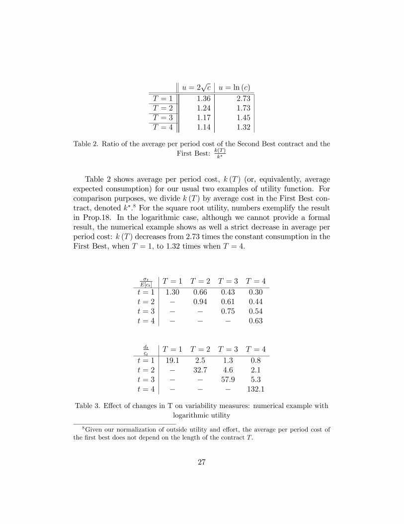
Table 2. Ratio of the average per period cost of the Second Best contract and theFirst Best: k(T )

k�

Table 2 shows average per period cost, k (T ) (or, equivalently, averageexpected consumption) for our usual two examples of utility function. Forcomparison purposes, we divide k (T ) by average cost in the First Best con-tract, denoted k�:8 For the square root utility, numbers exemplify the resultin Prop.18. In the logarithmic case, although we cannot provide a formalresult, the numerical example shows as well a strict decrease in average perperiod cost: k (T ) decreases from 2.73 times the constant consumption in theFirst Best, when T = 1; to 1.32 times when T = 4:

�tE[ct]

T = 1 T = 2 T = 3 T = 4

t = 1 1:30 0:66 0:43 0:30t = 2 � 0:94 0:61 0:44t = 3 � � 0:75 0:54t = 4 � � � 0:63

dtct

T = 1 T = 2 T = 3 T = 4

t = 1 19:1 2:5 1:3 0:8t = 2 � 32:7 4:6 2:1t = 3 � � 57:9 5:3t = 4 � � � 132:1

Table 3. E¤ect of changes in T on variability measures: numerical example withlogarithmic utility

8Given our normalization of outside utility and e¤ort, the average per period cost ofthe �rst best does not depend on the length of the contract T:

27

Table 3 presents (for logarithmic utility) quanti�cations of the e¤ect ofincreasing T on the two measures of variability of consumption presentedabove. Each column corresponds to a di¤erent length T; going from oneto four. All other parameters are kept equal to the values in the previousexamples. Looking at each row of the matrices, we can observe the e¤ect ofincreasing T in the variability measures corresponding to a given period t: Inthe �rst row of the �rst matrix, we see that the normalized standard deviationof consumption in period one, �1

E[c1]; falls from 1.3 to 0.3 when comparing a

one period long contract with a four period long contract, con�rming thepattern proved for the square root speci�cation in Prop19. In the secondmatrix, d1

c1follows the same pattern; it falls from 19.1 to 0.8.

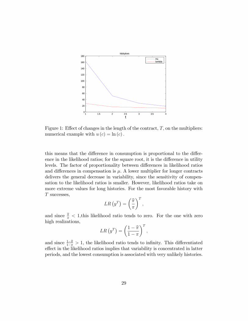
Di¤erences across contracts of di¤erent lengths respond to the better qual-ity of information, in the same way as the di¤erences across contracts withdi¤erent degrees of incentive problems reported in the previous section. Vari-ation in consumption is necessary for implementing high e¤ort. It is e¢ cientto concentrate most of this variation in longer histories for which relative like-lihoods are more informative. In particular, the bigger change in the scaleddt compared to that of the scaled �t is explained by the fact that dt measuresmaximum variation within a period, and not expected variation. For longhistories, the probability of the history associated with the minimum con-sumption ct becomes much smaller under the equilibrium e¤ort than underthe deviation. Punishments are exercised less often in equilibrium, loweringthe risk premium and thus reducing the cost of the contract.In Fig.1 the e¤ect on the multipliers of an increase in T is plotted for our

previous example with logarithmic utility. The sharper decrease correspondsto the multiplier of the IC, � (solid line). Although we only have a formalproof for u (c) =

pc; all of our numerical examples with CRRA utility, for

di¤erent degrees of risk aversion, obtain a decrease of � with T . This decreasein � means that, as the length of the contract increases, the IC is easier tosatisfy. The availability of better quality information is materialized in moreextreme values of the likelihood ratios. Rearranging the FOC�s of the SecondBest we have that for any two histories yt and eyet of any length,

1

u0 (c (yt))� 1

u0�c�eyet�� = �

0@cPr�eyet�

Pr�eyet� � Pr (ytjeL)

Pr (ytjeH)

1A :The patterns for the variability of compensation we just described can be un-derstood in terms of decrease of �: For the logarithmic utility, in particular,

28

1 1.5 2 2.5 3 3.5 40

20

40

60

80

100

120

140

160

180Multipliers

t

mulambda

Figure 1: E¤ect of changes in the length of the contract, T; on the multipliers:numerical example with u (c) = ln (c) :

this means that the di¤erence in consumption is proportional to the di¤er-ence in the likelihood ratios; for the square root, it is the di¤erence in utilitylevels. The factor of proportionality between di¤erences in likelihood ratiosand di¤erences in compensation is �: A lower multiplier for longer contractsdelivers the general decrease in variability, since the sensitivity of compen-sation to the likelihood ratios is smaller. However, likelihood ratios take onmore extreme values for long histories. For the most favorable history withT successes,

LR�yT�=

�b��

�T;

and since b��< 1;this likelihood ratio tends to zero. For the one with zero

high realizations,

LR�yT�=

�1� b�1� �

�T;

and since 1�b�1�� > 1, the likelihood ratio tends to in�nity. This di¤erentiated

e¤ect in the likelihood ratios implies that variability is concentrated in latterperiods, and the lowest consumption is associated with very unlikely histories.

29

5 Asymptotic Optimal Contract

Assume, as before, that output is distributed i.i.d. If the principal andthe agent can commit to an in�nite contractual relationship and utility isunbounded below (as in the logarithmic case) the cost of the contract undermoral hazard can get arbitrarily close to that of the First Best, i.e., underobservable e¤ort.When the contract lasts an in�nite number of periods, we have

U (1) =1

1� �U

e (1) =1

1� � e for e = feL; eHg :

The �rst best contract implies

c� = u�1 (U + eH)

and the �rst best cost is

K� (1) = 1

1� � c�:

The Second Best is not well de�ned for an in�nite number of periods. In thissection, we present an alternative feasible and incentive compatible contract,what we call a �one�step�contract. This contract is not necessarily optimal,but it is useful to study because we can get a bound on its cost. In thenext proposition we show that the cost of the �one�step�contract can getarbitrarily close to the cost of the First Best when contracts last an in�nitenumber of periods.A �one-step� contract is a tuple (c0; c; L) of two possible consumption

levels c0 and c plus a threshold L for the Likelihood Ratio. The contract isde�ned in the following way:

c(yt) =

�c0 if LR (yt) < Lc if LR (yt) � L :

Proposition 20 Assume output is distributed i.i.d. and the agent has a util-ity function that satis�es u (0) ! �1: For any � 2 (0; 1] and any " > 0;there exists a one-step contract (c0; c; L) such that the principal can imple-ment high e¤ort at a cost K (1) < K� (1) + ", where K� (1) is the costwhen e¤ort is observable.

30

Proof. We proof the result using utility levels, so �rst denote

u (c0) = u0 = u (c�) + �;

where c� is the level of consumption provided in the First Best, and

u (c) = u0 � P:

For a given L and for each possible date t; denote by At (L) the set includingall histories of length t such that their likelihood ratio is lower than thethreshold L; so they are assigned a consumption equal to c0: Denote byAct (L) the complement of that set:

At (L) =�yt j LR

�yt�� L

and

Act (L) =�yt j LR

�yt�> L

8t.

To any history yt 2 At a utility u0 is attached, while if yt 2 Act it is assignedu0�P: De�ne Ft (L) and bFt (L) as the total probability of observing a historyin At (L) for high and low e¤ort, correspondingly:

Ft (L) =X

yt2At(L)

Pr�ytjeH

�bFt (L) =

Xyt2At(L)

Pr�ytjeL

�:

The expected utility of the agent is

u01� � � P

Xt

�t�1 (1� Ft (L))�eH1� � :

For a given L we use the IC to determine the minimum punishment P thatmakes the contract incentive compatible:

�PXt

�t�1 (1� Ft (L))�eH1� � = �P

Xt

�t�1�1� bFt (L)�� eL

1� �

so we can write

P (L) =eH � eL

(1� �)P

t �t�1�Ft (L)� bFt (L)� :

31

Now we can write the PC as a function of L only, which will pin down u0 :

U + eH1� � =

u01� � � (eH � eL)

Pt �

t�1 (1� Ft (L))(1� �)

Pt �

t�1�Ft (L)� bFt (L)�

In other words, we can write the extra utility � that we have to provide overthe �rst best utility u (c�) explicitly as a function of L: Since u (c�) = U+eH ;

� (L) = (eH � eL)P

t �t�1 (1� Ft (L))P

t �t�1�Ft (L)� bFt (L)� : (3)

We can provide the following upper bound for the cost of the two-step con-tract:

K (1) < c01� � =

u�1 (u (c�) + � (L))

1� � :

The actual cost will be strictly lower than c01�� since, with probability (1� Ft (L)) >

0 the agent receives c. The �nal step of the proof is to show that when weincrease L not only we make the IC looser but also the PC, since � (T )is decreasing in L: When L increases,

Pt �

t�1 (1� Ft (L)) decreases. BothFt (L) and bFt (L) increase, but we can �nd a lower bound forPt �

t�1�Ft (L)� bFt (L)�

as a function of L: We show this by using the following inequality:

1� bFt (L)1� Ft (L)

� L

1� bFt (L) � L (1� Ft (L))1� bFt (L)� (1� Ft (L)) � L (1� Ft (L))� (1� Ft (L))

Ft (L)� bFt (L) � (1� Ft (L)) (L� 1) :

Going back to expression 3,

� (L) <1

L� 1 (eH � eL) (1� �)Xt

�t�1 (1� Ft (L)) :

By de�nition, 1� Ft (L) is decreasing in L for all t; so � (L) is decreasing inL as long as

Pt �

t�1�Ft (L)� bFt (L)� > 0 for L. From the above inequali-

ties, this will hold whenever 1� bFt (L) > 0 for some t: For the discrete case,32

this occurs if there exists a path yt such that L (yt) > L; which is guaranteedin the i.i.d. case. 9 Hence, for any " > 0 we can �nd an L low enough sothat K (1) < K� (1) + " :For a given L; there is a certain P (L) (decrease in utility) that needs to

be imposed so the contract is incentive compatible. When we increase L weare shrinking the sets Act (L) of histories that have that punishment attached.The probability of having to exercise P in equilibrium,

Pt �

t (1� Ft (L)) ; de-creases, so we need to increase P to still satisfy the IC. In the last step of theproof we show that, when we increase L; the decrease in

Pt �

t (1� Ft (L)) isbigger than the corresponding increase needed in P , so the expected punish-ment decreases, allowing us to decrease �. Showing that � (L) is decreasingin L is equivalent to establishing thatP

t �t�1 (1� Ft (L))P

t �t�1�Ft (L)� bFt (L)�

is decreasing in L: In other words, when the agent considers changing fromhigh to low e¤ort, the increase in the proportional probability of receiving apunishment increases with L:It should be noticed that for this result to hold unlimited punishment

power on the part of the principal is required, that is, that the utility of theagent can be made as low as wanted. Also, it is derived under the assumptionof extreme persistence of e¤ort, that is, i.i.d. output. This is in fact whatallows the quality of the information to keep on growing and reach levels thatpermit to tailor punishments so that they are almost surely not exercised inequilibrium.

6 Decrease in persistence of e¤ort

The i.i.d. assumption allows for a more complete characterization of thecontract, but it implies a very strong concept of e¤ort persistence. In thissection, we propose a modi�ed stochastic structure that still preserves thetractability of the solution, but relaxes the assumption of �perfect�persis-tence.

9This proof would go through for a more general assumption about the outout process,as long as this condition is met. Implicitely, the process of the output puts a lower boundon ":

33

The e¤ect of the action may now decrease as time passes. To modelthis e¤ect we need the probability distribution over the output levels to varywith time. We make the probability of observing yH a convex combinationof the e¤ort-determined probability, � or b�; and an exogenously determinedprobability (i.e., independent of the agent�s e¤ort choice), denoted by �:

Prt (yH jeH) = �t� + (1� �t)�Prt (yH jeL) = �tb� + (1� �t)�:

The sequence of weights, f�tgTt=1 with 0 � �t � 1 for every t, representsthe rate at which the e¤ect of e¤ort diminishes. This gives a measure ofpersistence of e¤ort: �t = 1 for all t corresponds to the i.i.d. case of perfectpersistence, while �t = 0 for all t implies that e¤ort does not a¤ect thedistribution of output. We consider a decreasing sequence for �t such that0 < �t < 1 for every t. The e¤ects of time on cost described in the previoussection still hold as long as �t > 0; i.e., as long as there is some informationcontained in new realizations, the principal is better o¤ when contracts arelonger. The asymptotic result still holds. Also, the changes in the propertiesof the contract with T are as described in Section 4.Lowering persistence worsens the quality of information available. The

e¤ect on cost parallels that of shortening the contract, as established in thefollowing proposition:

Proposition 21 Consider two possible persistence sequences (�1; :::; �T )and (�01; :::; �

0T ) where �t � �0t for all t: The cost of the contract is lower for

the problem with higher persistence, (�1; :::; �T ) :

Proof. Consider any two sequences of individual outcome probabilitiesfpt (yt)g ; fp0t (yt)g ; where p0t (yt) = tpt (yt) + (1� t) qt (yt) ; for 0 � t � 1and some Let P0 (y1; :::; yt) and P (y1; :::; yt) be the corresponding probabilitydistributions over histories for these processes with probabilities fp0tg andfptg, respectively. It follows that:

P0 (y1; :::; yt) = �j� jpj (yj) + (1� j)qj(yj)

�:

A typical element in the expansion of this product has the form:

��j2��f1;::;tgpj (yj)

34

where � is some coe¢ cient that varies with the subset � of terms considered(the constant term corresponds to � = ? :) This term can be obtained inte-grating out all histories that coincide on this subset of realizations fyjjj 2 �gand can thus be expressed as a linear combination of probabilities P (y1; :::; yt)for all these realizations: It follows that P0 (y1; :::; yt) is also a linear combi-nation of probabilities de�ned by P and thus the information system de�nedby P is su¢ cient for P0 and the corresponding implementation cost to theprincipal is lower. Now consider two information structures with same base-line probabilities but di¤erent weights (�1; :::; �T ) ; (�01; :::; �

0T ) where �t � �0t

for all t: Letting pt (yt) denote the probability de�ned by the �rst informa-tion structure and t = �0t=�t the previous result can be applied showingthat the the �rst information structure is su¢ cient for the second and thecorresponding cost of implementation lower.For the case of u (c) = 2

pc; we can derive implications for variability of

compensation. As in the case of changes in (� � b�) discussed in Prop.3, thee¤ect on individual period variance of compensation is not determined, sincevt varies with the level of persistence in every t:We can, however, show thatwhen persistence is higher compensation is less variable on average, whichbrings the cost of the contract down.

Proposition 22 Consider the case in which the agent has utility functionu (c) = 2

pc: Consider two possible persistence sequences (�1; :::; �T ) and

(�01; :::; �0T ) where �t � �0t for all t; with strict inequality for at least one t:

The cost of the contract and the average variance of utility are strictly lowerfor the problem with higher persistence, (�1; :::; �T ) :

Proof. Under this new speci�cation of the process for output, we have

E�LR

�yt�jeH�= 1 8t

and

E�LR

�yt�jeL�� bEt = Prt (yH jeL)2 + Prt (yH jeH)� 2Prt (yH jeL) Prt (yH jeH)

Prt (yH jeH) (1� Prt (yH jeH))

This expectation is increasing in Prt (yH jeH)� Prt (yH jeL) : The variance ofthe likelihood ratios at any t will be

vt =

tY�=1

bE� � 1;35

which is as well increasing in any of the Prt (yH jeH) � Prt (yH jeL) : Whencomparing the two persistence sequences, we can write

Prt (yH jeH)� Prt (yH jeL) = �t (� � b�)and, for the second sequence,

Pr0t (yH jeH)� Pr0t (yH jeL) = �0t (� � b�)Since �t � �0t ; it follows that vt � v0t for all t; with strict inequality for atleast one t; so the average variance of the Likelihood Ratios correspondingto the �rst sequence is strictly higher:

vT > v0T :

The expression for the variance of utility and its average across periods,as well as the expression for the average per period cost of the contract,are still as derived for the i.i.d. case (see the proof of Prop. 3). Both thesemeasures depend negatively on the average variance of the Likelihood Ratios,establishing the result.We present some numerical examples for logarithmic utility that illustrate

the same properties proved in the previous proposition. For these examples,we choose to have �t decrease exponentially:

�t = �t 8t:

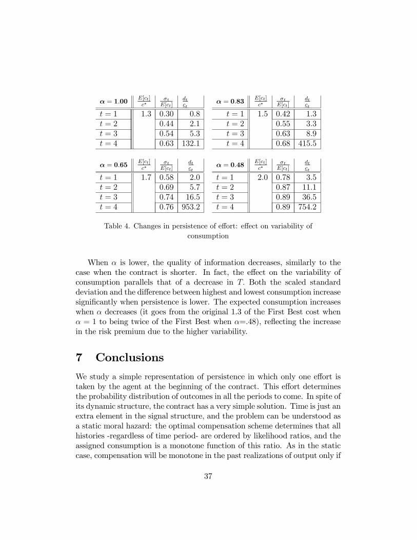
Fixing T = 4; we describe changes in the optimal contracts for the example ofTable 1 under di¤erent levels of persistence. Table 4 contains four matrices,with � ranging from 1 to 0.48; all other parameters are kept equal.

36

� = 1:00E[ct]c�

�tE[ct]

dtct

t = 1 1:3 0:30 0:8t = 2 0:44 2:1t = 3 0:54 5:3t = 4 0:63 132:1

� = 0:83E[ct]c�

�tE[ct]

dtct

t = 1 1:5 0:42 1:3t = 2 0:55 3:3t = 3 0:63 8:9t = 4 0:68 415:5

� = 0:65E[ct]c�

�tE[ct]

dtct

t = 1 1:7 0:58 2:0t = 2 0:69 5:7t = 3 0:74 16:5t = 4 0:76 953:2

� = 0:48E[ct]c�

�tE[ct]

dtct

t = 1 2:0 0:78 3:5t = 2 0:87 11:1t = 3 0:89 36:5t = 4 0:89 754:2

Table 4. Changes in persistence of e¤ort: e¤ect on variability ofconsumption

When � is lower, the quality of information decreases, similarly to thecase when the contract is shorter. In fact, the e¤ect on the variability ofconsumption parallels that of a decrease in T: Both the scaled standarddeviation and the di¤erence between highest and lowest consumption increasesigni�cantly when persistence is lower. The expected consumption increaseswhen � decreases (it goes from the original 1.3 of the First Best cost when� = 1 to being twice of the First Best when �=.48), re�ecting the increasein the risk premium due to the higher variability.

7 Conclusions

We study a simple representation of persistence in which only one e¤ort istaken by the agent at the beginning of the contract. This e¤ort determinesthe probability distribution of outcomes in all the periods to come. In spite ofits dynamic structure, the contract has a very simple solution. Time is just anextra element in the signal structure, and the problem can be understood asa static moral hazard: the optimal compensation scheme determines that allhistories -regardless of time period- are ordered by likelihood ratios, and theassigned consumption is a monotone function of this ratio. As in the staticcase, compensation will be monotone in the past realizations of output only if

37

likelihood ratios are so, i.e. if the monotone likelihood ratio property holds forall histories. Our characterization of the optimal contract has implications fordynamics of consumption. The inverse of the marginal utility of consumptionsatis�es the Rogerson condition: as in most dynamic problems with asymetricinformation, the agent is savings constraint and the evolution of his expectedconsumption through time depends on the concavity or convexity of theinverse of his marginal utility of consumption.When output realizations are i.i.d. over time, several conclusions are

reached relying on comparisons of the quality, or informativeness, of proba-bility distributions. Longer contracts have a lower cost of implementing highe¤ort, and a lower average variance of compensation across periods. Thecost of the contract approaches the �rst best as the number of time periodsgoes to in�nity. As persistence decreases, the variability of compensationincreases and so does the cost of implementation.

References

[1] Albuquerque, R. and H. Hopenhayn, 2004. "Optimal Lending Contractsand Firm Dynamics," Review of Economic Studies, vol. 71(2), pages285-315.

[2] Atkeson, A. �International Lending with Moral Hazard and Risk of Re-pudiation�, Econometrica, 59 (1991), 1069-1089.

[3] Fernandes, A. and C. Phelan. �A Recursive Formulation for RepeatedAgency with History Dependence,� Journal of Economic Theory, 91(2000): 223-247.

[4] Grochulski, B. and T. Piskorski. �Risky Human Capital and DeferredCapital Income Taxation." Mimeo (2006)

[5] Grossman, Sanford and Oliver D. Hart. �An Analysis of the Principal�Agent Problem.�Econometrica 51, Issue 1 (Jan.,1983), 7-46.

[6] Holmström, B. and P. Milgrom. �Aggregation and Linearity in the Pro-vision of Intertemporal Incentives�, Econometrica, 55, 303-328. (1987)

[7] Holmström, B. "Moral Hazard and Observability," Bell Journal of Eco-nomics, Vol. 10 (1) pp. 74-91. (1979)

38

[8] Holmström, B. �Managerial Incentive Problems: a Dynamic Perspec-tive.�Review of Economic Studies, 66, 169-182. (1999)

[9] Hopenhayn, H. and J.P. Nicolini: �Optimal Unemployment Insurance�,Journal of Political Economy, 105 (1997), 412-438.

[10] Jarque, A. �Repeated Moral Hazard with e¤ort Persistence", Mimeo(2005)

[11] Jarque, A. �Optimal CEO Compensation and Stock Options". Mimeo(2004)

[12] Kwon, I. �Incentives, Wages, and Promotions: Theory and Evidence�.Rand Journal of Economics, 37 (1), 100-120 (2006)

[13] Miller, Nolan.�Moral Hazard with Persistence and Learning�, Mimeo(1999)

[14] Mirrlees, James. �Notes on Welfare Economics, Information and Un-certainty�, in M. Balch, D. McFadden, and S. Wu (Eds.), Essays InEconomic Behavior under Uncertainty, pgs.. 243-258 (1974)

[15] Mukoyama, T. and A. Sahin, �Repeated Moral Hazard with Persis-tence,�Economic Theory, vol. 25(4), pages 831-854, 06 (2005)

[16] Phelan, C., Repeated Moral Hazard and One�Sided Commitment. J.Econ. Theory 66 (1995), 468-506.

[17] Rogerson, William P. �Repeated Moral Hazard", Econometrica, Vol. 53,No. 1. (1985), pp. 69-76.

[18] Shavell, S. and L. Weiss: �The Optimal Payment of UnemploymentInsurance Bene�ts over Time�, Journal of Political Economy, 87 (1979),1347-1362.

[19] Wang, C. �Incentives, CEO compensation, and Shareholder Wealth ina Dynamic Agency Model,� Journal of Economic Theory, 76, 72-105(1997)

39