Embed Size (px)
Citation preview

Monte Carlo Simulation of Radiation Transport
Agen-689Advances in Food Engineering

Introduction
Name Monte Carlo – created in 1940sNuclear scientists working on Los AlamosTo design a class of numerical methods based on the use of random numbersToday widely used to solve complex physical and math problems

The Monte Carlo Method
A technique of numerical analysisUses random sampling to construct the solution a problem
Find the value of π
Using geometry, it is easy to show that:Y
X1
1
(xi,yi)
The quadrant of a circleenclosed by a square having sides of 1
square in dots #area shaded in dots #4
414
1
square in dots #area shaded in dots #
2
2
=
==
π
ππ
r
r
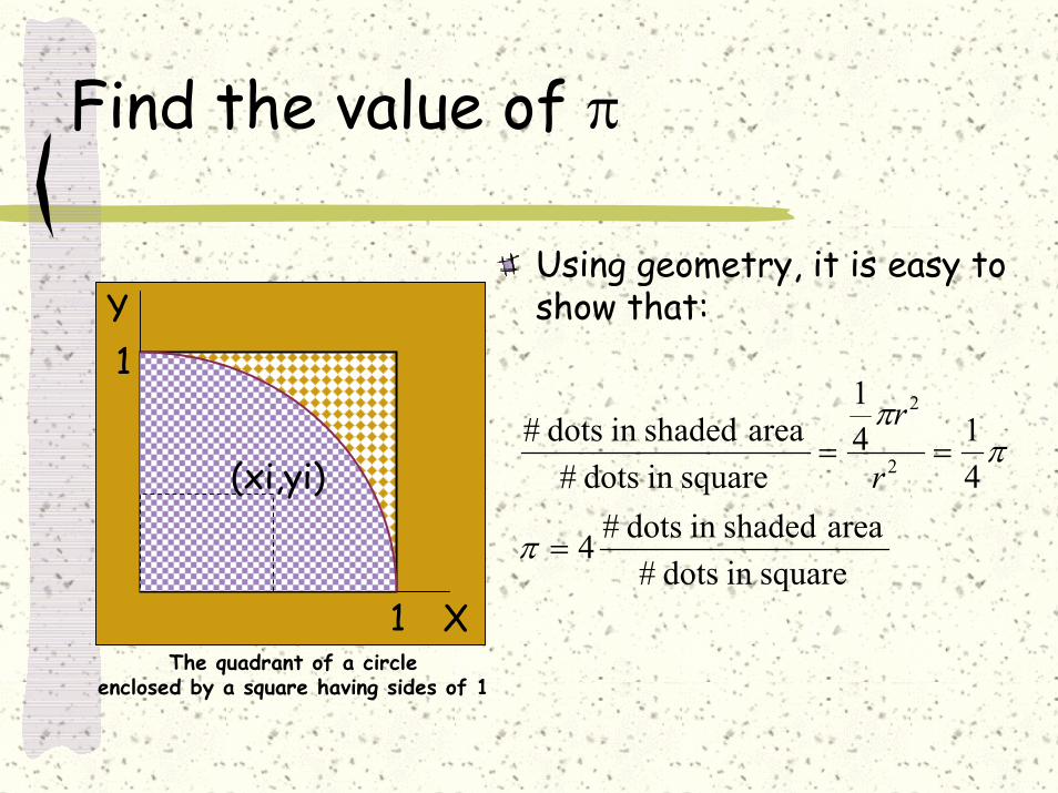
Find the value of π
Computer generates sequence of random numbers 0 < R < 1Pairs of random numbers (xi,yi) can be selected as values that determined point that lie in the squareFor each point one tests if
If so, the point lies inside the circleAfter a large number of random trials, π can be determined
Y
X1
1
(xi,yi)
The quadrant of a circleenclosed by a square having sides of 1
122 ≤+ ii yx
Find the value of π
x = (random #)y = (random #)dist = sqrt (x^2 +y^2)If dist < 1Let hits = hits +1
Do this thousands of times and π will be determinedSee spreadsheet
Radiation transport thru matter
Governed by attenuation coefficientsOr cross sectionsGiven the interaction probabilitiesThe use of linear attenuation coefficient describe the statistical nature of radiation penetration in matter

Consider photons, for example
The probability that a normally incident photon will reach the depth x in a material without interact is
x
xoeNxN µ−=)(
Narrow beamd
xexP µ−=)( RR>>d

In general
The probability that the first interaction of an incident photon will take place at a depth between x and x + dx is:
dxxPdxxP µ)()(1 =
The probability that it willreach the depth x
The probability that it willinteract in dx
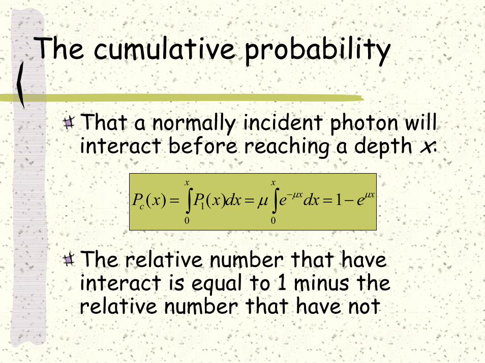
The cumulative probability
That a normally incident photon will interact before reaching a depth x:
The relative number that have interact is equal to 1 minus the relative number that have not
xx
xx
c edxedxxPxP µµµ −=== ∫∫ − 1)()(00
1

The cumulative probability
that a given incident photon has its first interaction before reaching a depth xThe linear attenuation coefficient is µ
Pc(x)
x0
1
xc exP µ−−= 1)(

Radiation transport simulation
From the knowledge of the numerical value of µ, we can also simulate radiation transport on a computer by using Monte Carlo procedures
Monte Carlo simulation of radiation transport
The history (track) of a particle is viewed as a random sequence of ‘free flights’The flights end with an interaction event In the event the particle changes its direction of movement, loses energy, and can produces secondary particles

Monte Carlo simulation of radiation transport
To simulate the random histories an interaction model – a set of differential cross sections (DCS) – is neededThe DSCs determine the probability distribution functions (PDF) of the random variables
Free path between successive interaction eventsKind of interactionEnergy loss and angular deflection

Monte Carlo simulation of radiation transport
Yields the same information as the solution of the Boltzmann transport equationWith the same interaction modelBut easier to implement

Monte Carlo simulation of radiation transport
The main drawback of this method lies on its random natureAll the results are affected by statistical uncertaintiesBut, can easily be solved by increasing the sampled population and computer time and variance-reduction techniques
Simulation of radiation transport
Considering Particle with energy E moving in a mediumHomogeneous ‘random scattering’ media

Simulation of radiation transport
Each interaction:Particle may lose energy WAnd/or change its direction of movement
Angular deflection determined by the scattering angle θAnd the azimuthal and φ

Simulation of radiation transport
Assuming that the particle can interact by 2 mechanisms A & B:
The scattering model is specified by the molecular DCSs:
);;( and );;(22
θσθσ WEdWddWE
dWdd BA
ΩΩ

Total CSs and PDFs
The total cross sections per molecule:
The PDFs of W and θ:
);;( sin2)(0 0
,2
BA, θσ
θθπσπ
WEdWdd
ddWEE
BA∫ ∫ Ω=
);;( )(
sin2);;( ,2
,, θ
σθσ
θπθ WEdWdd
dWdEWEp BA
BABA Ω
=

The PDF
Gives the (normalized) probability that in scattering event of type A:
The particle loses energy in the interval (W, W+dW)Is deflected into directions with polar angle in the interval (θ, θ+dθ)

The azimuthal scattering angle
In each collision it is uniformly distributed in the interval (0, 2π)
πφ
21)( =p

Generation of random tracks
Each particle starts off at a given position and energyThe state of the particle after an interaction is defined by:
Its position coordinates r = (x, y,z)Energy EDirection of flight, the component of vector d = (u, v, w)

Generation of random tracks
Each simulated track is caracterized by a series of states:
rn (position of the nth scattered event)En (energy after the event)dn (direction of movement after the event)
Generation of random tracks
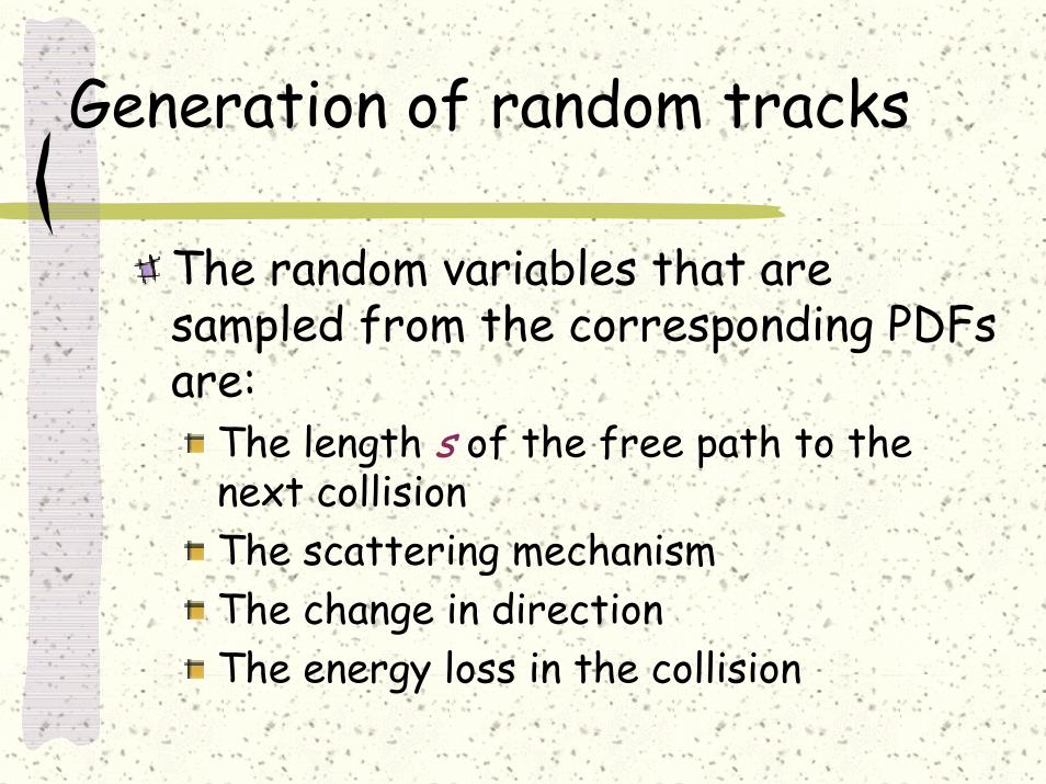
The random variables that are sampled from the corresponding PDFs are:
The length s of the free path to the next collisionThe scattering mechanismThe change in directionThe energy loss in the collision

The length of free path, s
Is distributed according to the PDF:
Random variables of s are generated by using the sampling equation:
The following interaction occurs at the position rn+1 = rn +sdn
)/exp()( 1 λλ ssp −=
ξλ ln−=s
ξ stands for random number uniformly distributedin the interval (0,1)

The type of interaction (A,B) and else
Is selected from point probabilities:
The energy loss W and θ are sampled from the distribution pA,B (E;W,θ)The azimuthal angle is generated as:
σσ
σσ B
AA
A pp == and
πξφ 2=

Angular deflections in single-scattering events
After sampling the values of W, θ and φ, The energy is reduced The direction after the interaction dn+1is obtained by performing a rotation of dn
x
z
y1ˆ +nr
),,(ˆ wvudn =
)',','(ˆ1 wvudn =+
θ
φ
The track simulation
The steps are repeatedThe track is finished when
It leaves the materialOr the E become smaller than a given Eabs (the energy is absorbed in the medium)
Example of Monte Carlo
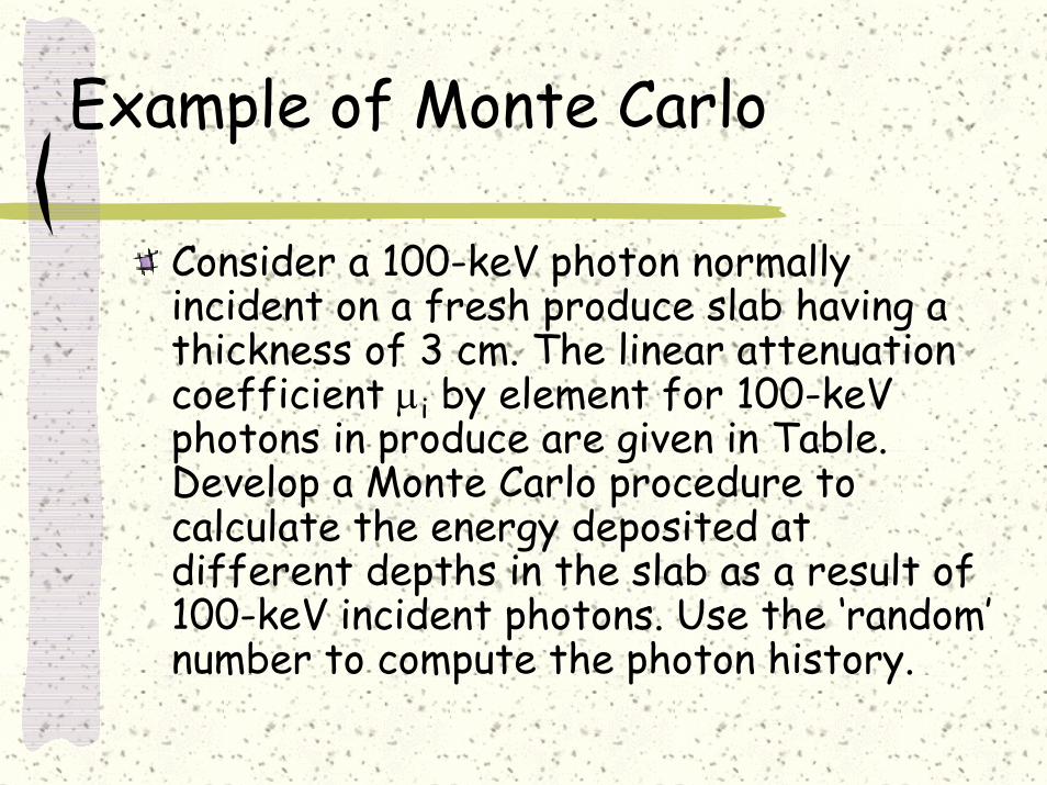
Consider a 100-keV photon normally incident on a fresh produce slab having a thickness of 3 cm. The linear attenuation coefficient µi by element for 100-keV photons in produce are given in Table. Develop a Monte Carlo procedure to calculate the energy deposited at different depths in the slab as a result of 100-keV incident photons. Use the ‘random’ number to compute the photon history.

Geometric arrangement
0xphoton
subslabs
dx

Data use to simulate photons transport
10.7538TOTAL
10.2020.1529N
0.7980.2010.1514C
0.5970.2060.1551O
0.3910.3910.2944H
Cumulative µi/µµi/µµi [cm-1]Element

Random Numbers
0.972685
0.103894
0.036213
0.686712
0.878101
Rii

Example
First select the first photon collision, based on the attenuation coef. for the photons of specific energy in the produceThis is accomplished by setting the cumulative probability of interaction equal to the first R1:
With 0 < R1 < 1.Solving for x (the location of the first collision)
11)( RexP xc =−= −µ
)1ln(11Rx −−=
µ

Example
So, from previous tables:
cmx 79.2)87810.01ln(7538.01
=−−=

Computer Simulators
EGSMCNPPENELOPE

EGS – Electron Gamma Shower
The Code was developed at Stanford University –Department of Nuclear PhysicsA general purpose package for the Monte Carlo simulation of the coupled transport of electrons and photons in an arbitrary geometry for particles with energies from a few keV up to several TeV. Some have referred to the EGS code as the de facto gold standard for clinical radiation dosimetry

MCNP – Monte Carlo N-Particle
Developed by Los Alamos National LabA code that can be used for neutron, photon, electron, or coupled neutron/photon/electron transport, including the capability to calculate eigenvalues for critical systems.The code treats an arbitrary three-dimensional configuration of materials in geometric cells bounded by first- and second-degree elliptical tori.

MCNP
Pointwise cross-section data are used. For photons
incoherent and coherent scattering, fluorescent emission after photoelectric absorption,absorption in pair production, bremsstrahlung.
A continuous-slowing-down model is used for electron transport that includes positrons, x-rays, and bremsstrahlung. Code include
Powerful general source, criticality source, and surface source;Geometry and output tally plotters; A collection of variance reduction techniques; A tally structure; Extensive collection of cross-section data.

PENELOPE
PENetration & Energy Loss of Positrons & ElectronsA code system for Monte Carlo simulation of electron and photon transportDeveloped by the Nuclear Energy Agency of the Organization for Economic Co-operation and Development

PENELOPE
It performs Monte Carlo simulation of coupled electron-photon transport in arbitrary materials and complex quadric geometries. Uses a mixed procedure for the simulation of electron and positron interactions (elastic scattering, inelastic scattering and bremsstrahlung emission)Photon interactions (Rayleigh scattering, Compton scattering, photoelectric effect and electron-positron pair production) and positron annihilation are simulated in adetailed way.

Simulation of Compton events
Assuming scattering by free electrons at rest
The PDF of cos θ and E’
),(')(sin2
2222
θθσ ESpFEcE
EEc
EEcr
dWdd
zA
−+
=
Ω
),(')(sin)',(cos 22
θθθ ESpFEcE
EEc
EEcEP z
−+
=

Simulation of Compton events
Integration of PDF over E’:
),(sin)(cos 22
θθθ ESEcE
EEc
EEcP
−+
=
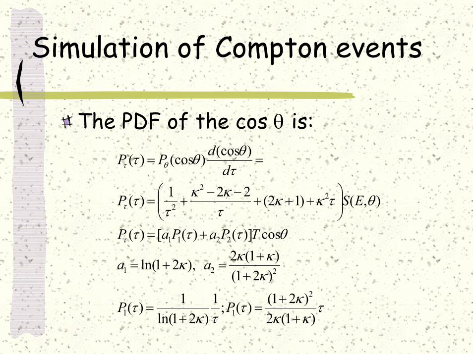
Simulation of Compton events
The PDF of the cos θ is:
τκκκτ
τκτ
κκκκ
θτττ
θτκκτκκ
ττ
τθθτ
τ
τ
θτ
)1(2)21()(;1
)21ln(1)(
)21()1(2 ),21ln(
cos)]()([)(
),()12(221)(
)(cos)(cos)(
2
11
221
2211
22
2
++
=+
=
++
=+=
+=
+++
−−+=
==
PP
aa
TPaPaP
ESP
ddPP

Simulation of Compton events
Random values for cos θ from the PDF can be generated as:
1 ;21
1/
)cos1(11
maxmin
2
=+
=
=
−+=≡
τκ
τ
κθκ
τ
mcEEEc

The algorithm to sample cosθ
Sample a value of the integer i (=1,2):
Sample τ using:21
2
21
1 )2( ;)1(aa
aaa
a+
=+
= ππ (point probabilities)
[ ]
=−+=
=2 if )1(1 if
2/12minmin
min
ii
τξττ
τ ξ
ξ

The algorithm to sample cosθ
Determine cos θ using:
Generate a new random number ξIf ξ>T(cosθ), go to step 1Deliver cosθ
11cosκττθ −
−=

The algorithm to sample cosθ
φ = 2πξEe = E – Ecφe = φ + πcosθe is:
λ = 1/(nσ)s = -λ*ξ
2
cos1/2
2
2
−++
=EcEmc
E-EcEmcE
eθ
Simulating
Using the algorithm described before we can generate the random walk of a photon incident in a wall Spreadsheet example