Embed Size (px)
Citation preview

Computer Physics Communications 218 (2017) 17–42
Contents lists available at ScienceDirect
Computer Physics Communications
journal homepage: www.elsevier.com/locate/cpc
Monte Carlo Particle Lists: MCPL✩
T. Kittelmann a,*, E. Klinkby b, E.B. Knudsen c, P. Willendrup c,a, X.X. Cai a,b, K. Kanaki aa European Spallation Source ERIC, Swedenb DTU Nutech, Technical University of Denmark, Denmarkc DTU Physics, Technical University of Denmark, Denmark
a r t i c l e i n f o
Article history:Received 9 September 2016Received in revised form 31 March 2017Accepted 20 April 2017Available online 8 May 2017
Keywords:MCPLMonte Carlo simulationsParticle storageFile formatGeant4MCNPMcStasMcXtrace
a b s t r a c t
A binary formatwith lists of particle state information, for interchanging particles between variousMonteCarlo simulation applications, is presented. Portable C code for file manipulation is made available to thescientific community, along with converters and plugins for several popular simulation packages.Program summaryProgram Title:MCPLProgram Files doi: http://dx.doi.org/10.17632/cby92vsv5g.1Licensing provisions: CC0 for core MCPL, see LICENSE file for details.Programming language: C and C++External routines/libraries: Geant4, MCNP, McStas, McXtraceNature of problem: Saving particle states in Monte Carlo simulations, for interchange between simulationpackages or for reuse within a single package.Solution method: Binary interchange format with associated code written in portable C along with toolsand interfaces for relevant simulation packages.
© 2017 The Authors. Published by Elsevier B.V. This is an open access article under the CC BY license(http://creativecommons.org/licenses/by/4.0/).
1. Introduction
The usage of Monte Carlo simulations to study the transport and interaction of particles and radiation is a powerful and populartechnique, finding use throughout a wide range of fields — including but not limited to both high energy and nuclear physics, as wellas space and medical sciences [1]. Naturally, a plethora of different frameworks and applications exist for carrying out these simulations(cf. Section 3 for examples), with implementations in different languages and domains ranging from general purpose to highly specialisedfield- and application-specific.
A common principle used in the implementation of these applications is the representation of particles by a set of state parameters –usually including at least particle type, time coordinate, position and velocity or momentum vectors – and a suitable representation ofthe geometry of the problem (either via descriptions of actual surfaces and volumes in a virtual three-dimensional space, or throughsuitable parameterisations). In the simplest scenario where no variance-reduction techniques are employed, simulations are typicallycarried out by proceeding iteratively in steps from an initial set of particles states, with the state information being updated along theway as a result of the pseudo-random or deterministic modelling of processes affecting the particle. The modelling can represent particleself-interactions, interactions with the material of the simulated geometry, or simply its forward transport through the geometry, usingeither straight-forward ray-tracing techniques or more complicated trajectory calculations as appropriate. In addition to a simple updateof state parameters, the modelling can result in termination of the simulation for the given particle or in the creation of new secondaryparticle states, which will in turn undergo simulation themselves.
Occasionally, use-cases arise in which it would be beneficial to be able to capture a certain subset of particle states present in a givensimulation, in order to continue their simulation at a later point in either the same or a different framework. Such capabilities have typicallybeen implemented using custom application-specific means of data exchange, often involving the tedious writing of custom input andoutput hooks for the specific frameworks and use-cases in question. Here is instead presented a standard format for exchange of particle
✩ This paper and its associated computer program are available via the Computer Physics Communication homepage on ScienceDirect (http://www.sciencedirect.com/science/journal/00104655).* Corresponding author.
E-mail address: [email protected] (T. Kittelmann).
http://dx.doi.org/10.1016/j.cpc.2017.04.0120010-4655/© 2017 The Authors. Published by Elsevier B.V. This is an open access article under the CC BY license (http://creativecommons.org/licenses/by/4.0/).
18 T. Kittelmann et al. / Computer Physics Communications 218 (2017) 17–42
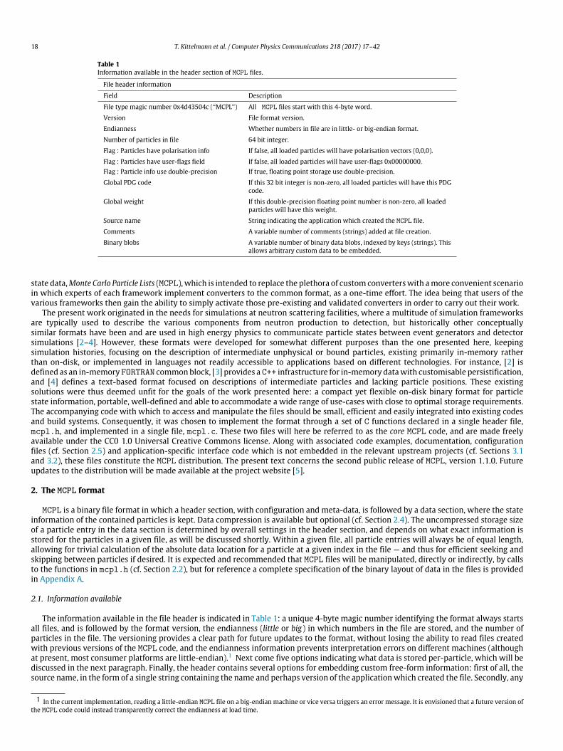
Table 1Information available in the header section of MCPL files.
File header information
Field Description
File type magic number 0x4d43504c (‘‘MCPL’’) All MCPL files start with this 4-byte word.
Version File format version.
Endianness Whether numbers in file are in little- or big-endian format.
Number of particles in file 64 bit integer.
Flag : Particles have polarisation info If false, all loaded particles will have polarisation vectors (0,0,0).
Flag : Particles have user-flags field If false, all loaded particles will have user-flags 0x00000000.Flag : Particle info use double-precision If true, floating point storage use double-precision.
Global PDG code If this 32 bit integer is non-zero, all loaded particles will have this PDGcode.
Global weight If this double-precision floating point number is non-zero, all loadedparticles will have this weight.
Source name String indicating the application which created the MCPL file.
Comments A variable number of comments (strings) added at file creation.
Binary blobs A variable number of binary data blobs, indexed by keys (strings). Thisallows arbitrary custom data to be embedded.
state data,Monte Carlo Particle Lists (MCPL), which is intended to replace the plethora of custom converterswith amore convenient scenarioin which experts of each framework implement converters to the common format, as a one-time effort. The idea being that users of thevarious frameworks then gain the ability to simply activate those pre-existing and validated converters in order to carry out their work.
The present work originated in the needs for simulations at neutron scattering facilities, where a multitude of simulation frameworksare typically used to describe the various components from neutron production to detection, but historically other conceptuallysimilar formats have been and are used in high energy physics to communicate particle states between event generators and detectorsimulations [2–4]. However, these formats were developed for somewhat different purposes than the one presented here, keepingsimulation histories, focusing on the description of intermediate unphysical or bound particles, existing primarily in-memory ratherthan on-disk, or implemented in languages not readily accessible to applications based on different technologies. For instance, [2] isdefined as an in-memoryFORTRAN commonblock, [3] provides aC++ infrastructure for in-memory datawith customisable persistification,and [4] defines a text-based format focused on descriptions of intermediate particles and lacking particle positions. These existingsolutions were thus deemed unfit for the goals of the work presented here: a compact yet flexible on-disk binary format for particlestate information, portable, well-defined and able to accommodate a wide range of use-cases with close to optimal storage requirements.The accompanying code with which to access and manipulate the files should be small, efficient and easily integrated into existing codesand build systems. Consequently, it was chosen to implement the format through a set of C functions declared in a single header file,mcpl.h, and implemented in a single file, mcpl.c. These two files will here be referred to as the core MCPL code, and are made freelyavailable under the CC0 1.0 Universal Creative Commons license. Along with associated code examples, documentation, configurationfiles (cf. Section 2.5) and application-specific interface code which is not embedded in the relevant upstream projects (cf. Sections 3.1and 3.2), these files constitute the MCPL distribution. The present text concerns the second public release of MCPL, version 1.1.0. Futureupdates to the distribution will be made available at the project website [5].
2. The MCPL format
MCPL is a binary file format in which a header section, with configuration and meta-data, is followed by a data section, where the stateinformation of the contained particles is kept. Data compression is available but optional (cf. Section 2.4). The uncompressed storage sizeof a particle entry in the data section is determined by overall settings in the header section, and depends on what exact information isstored for the particles in a given file, as will be discussed shortly. Within a given file, all particle entries will always be of equal length,allowing for trivial calculation of the absolute data location for a particle at a given index in the file — and thus for efficient seeking andskipping between particles if desired. It is expected and recommended that MCPL files will be manipulated, directly or indirectly, by callsto the functions in mcpl.h (cf. Section 2.2), but for reference a complete specification of the binary layout of data in the files is providedin Appendix A.
2.1. Information available
The information available in the file header is indicated in Table 1: a unique 4-byte magic number identifying the format always startsall files, and is followed by the format version, the endianness (little or big) in which numbers in the file are stored, and the number ofparticles in the file. The versioning provides a clear path for future updates to the format, without losing the ability to read files createdwith previous versions of the MCPL code, and the endianness information prevents interpretation errors on different machines (althoughat present, most consumer platforms are little-endian).1 Next come five options indicating what data is stored per-particle, which will bediscussed in the next paragraph. Finally, the header contains several options for embedding custom free-form information: first of all, thesource name, in the form of a single string containing the name and perhaps version of the applicationwhich created the file. Secondly, any
1 In the current implementation, reading a little-endian MCPL file on a big-endian machine or vice versa triggers an error message. It is envisioned that a future version ofthe MCPL code could instead transparently correct the endianness at load time.

T. Kittelmann et al. / Computer Physics Communications 218 (2017) 17–42 19
Table 2Particle state information available and uncompressed storage requirements for each entry in the data section of MCPLfiles.
Particle state information
Field Description Bytes of storage used per entry (FP = 4 or 8 bytes)
PDG code 32 bit integer indicating particle type. 0 or 4Position Vector, values in centimetres. 3FPDirection Unit vector along the particle momentum. 2FPKinetic energy Value in MeV. 1FPTime Value in milliseconds. 1FPWeight Weight or intensity. 0 or 1FPPolarisation Vector. 0 or 3FPUser-flags 32 bit integer with custom info. 0 or 4
number of strings can be added as human readable comments, and, thirdly, any number of binary data blobs can be added, each identifiedby a string key. The MCPL format itself provides no restrictions on what data, if any, can be stored in these binary blobs, but useful contentcould for instance be a copy of configuration data used by the source applicationwhen the given file was produced, kept for later reference.Also note that, for reasons of security, no code in the MCPL distribution ever attempts to interpret contents stored in such binary datablobs.
Table 2 shows the state information available per-particle in MCPL files, along with the storage requirements of each field. Particleposition, direction, kinetic energy and time are always stored.2 Polarisation vectors and so-called user-flags in the form of unsigned 32bit integers are only stored when relevant flags in the header are enabled and weights are only stored explicitly in each entry when noglobal common value was set in the header. Likewise, the particle type information in the form of so-called PDG codes is only storedwhen a global PDG code was not specified in the header. The PDG codes must follow the scheme developed by the Particle Data Group in[6, ch. 42], which is inarguably the most comprehensive and widely adopted standard for particle type encoding in simulations. Finally,again depending on a flag in the header, particle information uses either single- (4 bytes) or double-precision (8 bytes) storage for floatingpoint numbers. All in all, summing up the numbers in the last column of Table 2, particles are seen to consume between 28 and 96 bytes ofuncompressed storage space per entry. The MCPL format is thus designed to be flexible enough to handle use-cases requiring a high levelof detail in the particle state information, without imposing excessive storage requirements on less demanding scenarios.
Note that while the units for position, energy and time indicated in Table 2 of course must be respected, the choices themselves aresomewhat arbitrary and should in no way be taken to indicate the suitability of the MCPL format for a given simulation task. In particular,note that within the dynamic range of a given floating point representation, the relative numerical precision is essentially independent ofthe magnitude of the numbers involved and is determined by the number of bits allocated for the significand [7]. Thus, it is important torealise that usage of the MCPL format to deal with a simulation task whose natural units are many orders of magnitude different than theones in Table 2 does not imply any detrimental impact on numerical precision.
Packing of the three-dimensional unit directional vector into just two floating point numbers of storage is carried out via a newpacking algorithm, tentatively namedAdaptive Projection Packing, discussed in detail in Appendix B. Unlike other popular packing strategiesconsidered, the chosen algorithm provides what is for all practical purposes flawless performance, with a precision comparable to the oneexisting absent any packing (i.e. direct storage of all coordinates into three floating point numbers). It does so without suffering fromdomain validity issues, and the implemented code is not significantly slower to execute than the alternatives.
2.2. Accessing or creating MCPL files programmatically
While a complete documentation of the programming API provided by the implementation of MCPL in mcpl.h and mcpl.c can befound in Appendix C, the present discussion will restrict itself to a more digestible overview.
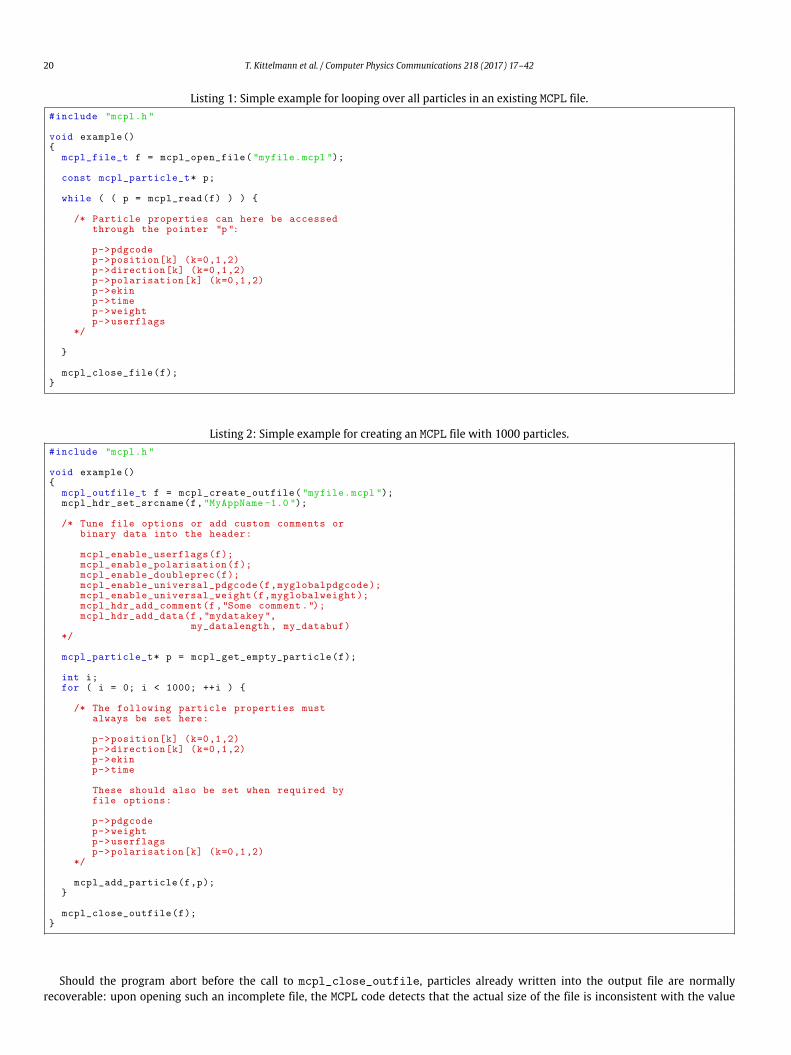
The main feature provided by the API is naturally the ability to create new MCPL files and access the contents of existing ones, usinga set of dedicated functions. No matter which settings were chosen when a given MCPL file was created, the interface for accessing theheader and particle state information within it is the same, as can be seen in Listing 1: after obtaining a file handle via mcpl_open_file,a pointer to an mcpl_particle_t struct, whose fields contain the state information available for a given particle, is returned by callingmcpl_read. This also advances the position in the file, and returns a null-pointer when there are no more particles in the file, ending theloop. If a file was created with either polarisation vectors or user-flags disabled, the corresponding fields on the particle will contain zeros(thus representing polarisation information with null-vectors and user-flags with an integer with no bits enabled). All floating point fieldson mcpl_particle_t are represented with a double-precision type, but the actual precision of the numbers will obviously be limitedto that stored in the input file. In addition to the interface illustrated by Listing 1, functions can be found in mcpl.h for accessing anyinformation available in the file header (see Table 1), or for seeking and skipping to particles at specific positions in the file, rather thansimply iterating through the full file.
Code creating MCPL files is typically slightly more involved, as the creation process also involves deciding on the values of the variousheader flags and filling of free-form information like source name and comments. An example producing a filewith 1000 particles is shownin Listing 2. The first part of the procedure is to obtain a file handle through a call to mcpl_create_outfile, configure the header andoverall flags, and prepare a zero-initialised instance of mcpl_particle_t. Next comes the loop filling the particles into the file, whichhappens by updating the state information on the mcpl_particle_t instance as needed, and passing it to mcpl_add_particle eachtime. At the end, a call to mcpl_close_outfile finishes up by flushing all internal buffers to disk and updating the field containing thenumber of particles at the beginning of the file.
2 Note that a valid alternative to storing the directional unit vector along with the kinetic energy would have been the momentum vector. However, the choice here isconsistent with the variables used in interfaces of both MCNP and Geant4, and means that the mcpl2ssw converter discussed in Section 3.2 can be implemented withoutaccess to an unwieldy database of particle and isotope masses.
20 T. Kittelmann et al. / Computer Physics Communications 218 (2017) 17–42
Listing 1: Simple example for looping over all particles in an existing MCPL file.#include " mcpl.h "
void example(){
mcpl_file_t f = mcpl_open_file( " myfile.mcpl " );
const mcpl_particle_t* p;
while ( ( p = mcpl_read(f) ) ) {
/* Particle properties can here be accessedthrough the pointer " p ":
p->pdgcodep->position[k] (k=0,1,2)p->direction[k] (k=0,1,2)p->polarisation[k] (k=0,1,2)p->ekinp->timep->weightp->userflags
*/
}
mcpl_close_file(f);}
Listing 2: Simple example for creating an MCPL file with 1000 particles.#include " mcpl.h "
void example(){
mcpl_outfile_t f = mcpl_create_outfile( " myfile.mcpl " );mcpl_hdr_set_srcname(f, " MyAppName -1.0 " );
/* Tune file options or add custom comments orbinary data into the header:
mcpl_enable_userflags(f);mcpl_enable_polarisation(f);mcpl_enable_doubleprec(f);mcpl_enable_universal_pdgcode(f,myglobalpdgcode);mcpl_enable_universal_weight(f,myglobalweight);mcpl_hdr_add_comment(f ," Some comment .");mcpl_hdr_add_data(f ," mydatakey " ,
my_datalength , my_databuf)*/
mcpl_particle_t* p = mcpl_get_empty_particle(f);
int i;for ( i = 0; i < 1000; ++i ) {
/* The following particle properties mustalways be set here:
p->position[k] (k=0,1,2)p->direction[k] (k=0,1,2)p->ekinp->time
These should also be set when required byfile options:
p->pdgcodep->weightp->userflagsp->polarisation[k] (k=0,1,2)
*/
mcpl_add_particle(f,p);}
mcpl_close_outfile(f);}
Should the program abort before the call to mcpl_close_outfile, particles already written into the output file are normallyrecoverable: upon opening such an incomplete file, the MCPL code detects that the actual size of the file is inconsistent with the value

T. Kittelmann et al. / Computer Physics Communications 218 (2017) 17–42 21
Listing 3: Example extracting low-energy neutrons (PDG code 2112) from an MCPL file.#include " mcpl.h "
void example() {
/* open files, transfer meta-data, add comment */
mcpl_file_t fi = mcpl_open_file( " myfile.mcpl " );mcpl_outfile_t fo = mcpl_create_outfile( " new.mcpl " );mcpl_transfer_metadata(fi, fo);mcpl_hdr_add_comment(fo, " Extracted neutrons with ekin <0.1MeV " );
/* transfer selected particles */
const mcpl_particle_t* particle;while ( ( particle = mcpl_read(fi) ) ) {
if ( particle ->pdgcode == 2112 && particle ->ekin < 0.1 )mcpl_add_particle(fo,particle);
}
/* finish up */
mcpl_close_outfile(fo);mcpl_close_file(fi);
}
of the field in the header containing the number of particles. Thus, it emits a warning message and calculates a more appropriate valuefor the field, ignoring any partially written particle state entry at the end of the file. This ability to transparently correct incomplete filesupon load also means that it is possible to inspect (with the mcpltool command discussed in Section 2.3) or analyse files that are stillbeing created. To avoid seeing a warning each time a file left over from an aborted job is opened, mcpl.h also provides the functionmcpl_repairwhich can be used to permanently correct the header of the file.
Likewise, mcpl.h also provides the function mcpl_merge_files which can be used to merge a list of compatible MCPL files intoa new one, which might typically be useful when gathering up the output of simulations carried out via parallel processing techniques.Compatibility heremeans that the filesmust have essentially identical header sections, except for the field holding the number of particles.Finally, the function mcpl_transfer_metadata can be used to easily implement custom extraction of particle subsets from existingMCPL files into new (smaller) ones. An example of this is illustrated in Listing 3.
2.3. Accessing MCPL files from the command line
Compared with simpler text-based formats (e.g. ASCII files with data formatted in columns), one potential disadvantage of a binarydata format like MCPL is the lack of an easy way for users to quickly inspect a file and investigate its contents. To alleviate this,mcpl.h provides a function which, in a straight-forward manner, can be used to build a generic mcpltool command-line executable:int mcpl_tool(int argc,char** argv), for which full usage instructions can be found in Appendix D or by invoking it with the--help flag. Simply running this command on an MCPL file without specifying other arguments, results in a short summary of the filecontent being printed to standard output, which includes a listing of the first 10 contained particles. An example of such a summary isprovided in Listing 4: it is clear from the displayedmeta-data that the particles in the given file represent a transmission spectrum resultingfrom illumination of a block of lead by a 10 GeV proton beam in a Geant4 [8,9] simulation. The displayed header information and datacolumns should be mostly self-explanatory, noting that (x, y, z) indicates the particle position, (ux, uy, uz) its normalised direction, andthat the pdgcode column indeed shows particle types typical in a hadronic shower: π+ (211), γ (22), protons (2212), π− (−211) andneutrons (2112). If the file had user-flags or polarisation vectors enabled, appropriate columns for those would be shown as well. Finally,note that the 36 bytes/particle refers to uncompressed storage, and that in this particular case the file actually has a compressionratio of approximately 70%, meaning that about 25 bytes of on-disk storage is used per particle (cf. Section 2.4).
By providing suitable arguments (cf. Appendix D) to mcpltool, it is possible to modify what information from the file is displayed.This includes the possibility to change what particles from the file, if any, should be listed, as well as the option to extract the contents ofa given binary data blob to standard output. The latter might be particularly handy when entire configuration files have been embedded(cf. Sections 3.2 and 3.3). Finally, the mcpltool command also allows file merging and repairing, as discussed in Section 2.2, and providesfunctionality for selecting a subset of particles from a given file and extracting them into a new smaller file.
Advanced functionality such as graphics display and interactive GUI-based investigation or manipulation of the contents of MCPL filesis not provided by the mcpltool, since those would imply additional unwanted dependencies to the core MCPL code, which is requiredby design to be light-weight and widely portable. However, it is the hope that the existence of a standard format like MCPLwill encouragedevelopment of such tools, and indeed some already exist in the in-house framework [10] of the Detector Group at the European SpallationSource (ESS) [11,12]. It is intended for a future distribution of MCPL to include relevant parts of these tools as a separate and optionalcomponent.
2.4. Compression
The utilisation of data compression in a format like MCPL is potentially an important feature, since on-disk storage size could be aconcern for some applications. Aiming to maximise flexibility, transparency and portability, optional compression of MCPL files is simplyprovided by allowingwhole-file compression into thewidespread GZIP format [13] (changing the file extension from .mcpl to .mcpl.gz

22 T. Kittelmann et al. / Computer Physics Communications 218 (2017) 17–42
Listing4:
Exam
pleou
tput
ofru
nningmc
plto
olwith
noargu
men
tson
asp
ecificMC
PLfile.
Opened
MCPL
file
myoutput.mcpl.gz
:
Basic
info
Format
:MC
PL-3
No.
ofparticles
:1106933
Header
storage
:140
bytes
Data
storage
:39849588
bytes
Custom
meta
data
Source
:"G
4MCPLWriter
[G4MCPLWriter]"
Number
ofcomments
:1
->
comment
0:
"Transmission
spectrum
from
10GeV
proton
beam
on20
cmlead"
Number
ofblobs
:0
Particle
data
format
User
flags
:no
Polarisation
info
:no
Fixed
part.
type
:no
Fixed
part.
weight
:no
FPprecision
:single
Endianness
:little
Storage
:36
bytes/particle
index
pdgcode
ekin[MeV]
x[cm
]y[cm
]z[cm
]ux
uyuz
time[ms
]weight
0211
487.02
-0.5898
1.835
20-0.092407
0.20491
0.97441
7.3346e-07
11
221.5326
1.0635
11.351
200.080441
0.66026
0.74672
1.0882e-06
12
223.9526
-0.43907
8.6473
20-0.56616
0.50558
0.65104
1.0286e-06
13
220.82591
1.7444
9.7622
200.092099
0.79597
0.59829
1.0378e-06
14
221.1958
2.1806
8.6416
200.21997
0.66435
0.71432
1.0124e-06
15
221.2525
3.0949
7.7366
200.48903
0.30789
0.81612
1.013e-06
16
222.6247
3.948
5.681
200.62503
0.64221
0.44374
9.1152e-07
17
2212
824.28
-1.8797
-2.5124
20-0.3077
-0.40496
0.861
7.6539e-07
18
-211
3459.8
-0.79521
0.91481
20-0.13441
0.14438
0.98035
7.0618e-07
19
2112
0.30553
54.471
33.386
200.4862
0.011958
0.87377
0.00016442
1

T. Kittelmann et al. / Computer Physics Communications 218 (2017) 17–42 23
in the process). This utilises the DEFLATE compression algorithm [14] which offers a good performance compromise with a reasonablecompression ratio and an excellent speed of compression and decompression.
Relying on a standard format such as GZIP means that, if needed, users can avail themselves of existing tools (like the gzip andgunzip commands available on most UNIX platforms) to change the compression state of an existing MCPL file. However, when the codein mcpl.c is linkedwith the ubiquitous ZLIB [15,16] (cf. Section 2.5), compressed MCPL files can be read directly. For convenience, mcpl.hadditionally provides a function mcpl_closeandgzip_outfile, which can be used instead of mcpl_close_outfile (cf. Listing 2) toensure that newly created MCPL files are automatically compressed if possible (either through a call to an external gzip command orthrough custom ZLIB-dependent code, depending on availability).
2.5. Build and deployment
It is the hope that eventually MCPL capabilities will be included upstream in many applications, and that users of those consequentlywill not have to do anything extra to start using it. As will be discussed in Section 3, this is at present the case for users of recent versionsof McStas [17,18] and McXtrace [19], and is additionally the case for users of the in-house Geant4-based framework of the ESS DetectorGroup [10].
By design, it is expected that most developers wishing to add MCPL support to their application will simply place copies of mcpl.hand mcpl.c into their existing build system and include mcpl.h from either C or C++ code.3 In order to make the resulting binary codeable to manipulate compressed files directly (cf. Section 2.4), the code in mcpl.c must usually be compiled against and linked with aninstallation of ZLIB (see detailed instructions regarding build flags at the top of mcpl.c). Alternatively, the MCPL distribution presentedhere contains a ‘‘fat’’ auto-generated drop-in replacement for mcpl.c named mcpl_fat.c, in which the source code of ZLIB has beenincluded in its entirety.4 Using this somewhat larger file enables ZLIB-dependent code in MCPL even in situations where ZLIBmight notbe otherwise available.
In addition to the core MCPL code, the MCPL distribution also contains a small file providing the mcpltool executable, C++ filesimplementing the Geant4 classes discussed in Section 3.1, C files for the mcpl2ssw and ssw2mcpl executables discussed in Section 3.2,and a few examples show-casing how user code might look.
Building of all of these parts should be straight-forward using standard tools, but a configuration file for CMake [20] which buildsand installs everything is nonetheless provided for reference and convenience. Additionally, ‘‘fat’’ single-file versions of all command lineutilities (mcpltool, mcpl2ssw and ssw2mcpl) are also provided, containing both MCPL and ZLIB code within as appropriate. Thus, anyof these single-file versions can be compiled directly into the corresponding command line executable, without any other dependenciesthan a C compiler. For more details about how to build and deploy, refer to the INSTALL file shipped with the MCPL distribution.
3. Application-specific converters and plugins
While the examples in Section 2.2 show how it is possible to manipulate MCPL files directly from C or C++ code, it is not envisionedthat most users will have to write such code themselves. Rather, in addition to using available tools (such as the mcpltool describedin Section 2.3) to access the contents of files as needed, users would ideally simply use pre-existing plugins and converters written byapplication-specific experts, to load particles from MCPL files into their givenMonte Carlo applications, or extract particles from those intoMCPL files. At the time of this initial public release of MCPL, four such applications are already MCPL-aware in this manner: Geant4, MCNP,McStas and McXtrace, and the details of the corresponding converters and plugins are discussed in the following sub-sections, after afew general pieces of advice for other implementers in the next paragraphs.
In order for MCPL files to be as widely exchangeable as possible, code loading particles from MCPL files into a given Monte Carloapplication should preferably be as accepting as possible. In particular, this means that warnings rather than errors should result if theinput file contains PDG codes corresponding to particle types that cannot be handled by the application in question. As an example, adetailed MCNP or Geant4 simulation of a moderated neutron source will typically produce files containing not only neutrons, but alsogammas and other particles. It should certainly be possible to load such a file into a neutron-only simulation application like McStas,resulting in simulation of the contained neutrons (preferably with a warning or informative message drawing attention to some particlesbeing ignored).
Applications employing parallel processing techniques, must always pay particular attention when implementing file-based I/O, andthis is naturally also the case when creating MCPL-aware plugins for them. However, the available functionality for merging of MCPL filesmakes the scenario of file creation particularly simple to implement: each sub-task can simply write its own file, with the subsequentmerging into a single file taking place during post-processing. For reading of particles in existing MCPL files, it is recommended that eachsub-task performs a separate call to mcpl_open_file, and use the skipping and seeking functionality to load just a subset of the particleswithin, as required. In the case of a multi-threading application, it is of course also possible to handle concurrent input or output directlythrough a single file handle. In this case, however, calls to mcpl_add_particle and mcpl_read must be protected against concurrentinvocations with a suitable lock or mutex.
The following three sub-sections are dedicated to discussions of presently available MCPL interfaces for specific Monte Carlo applica-tions. The discussions will in each case presuppose familiarity with the application in question.
3 Compilation of mcpl.c can happen with any of the following standards: C99, C11, C++98, C++11, C++14, or later. In addition to those, mcpl.h is also C89 compatible.Note that on platforms where the standard Cmath function sqrt is provided in a separate library, that library must be available at link-time.4 Note that all ZLIB symbols have been prefixed, to guard against potential run-time clashes where a separate ZLIB is nonetheless loaded.

24 T. Kittelmann et al. / Computer Physics Communications 218 (2017) 17–42
Listing 5: The G4MCPLGenerator class.class G4MCPLGenerator : public G4VUserPrimaryGeneratorAction{
public:
G4MCPLGenerator(const G4String& inputFile);virtual ~G4MCPLGenerator();virtual void GeneratePrimaries(G4Event*);
protected:
//Reimplement this to filter input particles (default//implementation accepts all particles):virtual bool UseParticle(const mcpl_particle_t*) const;
//Reimplement this to change coordinates or weights of//input particles before using them (does nothing by//default):virtual void ModifyParticle(G4ThreeVector& position,
G4ThreeVector& direction ,G4ThreeVector& polarisation ,G4double& time,G4double& weight) const;
private:// ..
};
Listing 6: Example showing how to load particles from an MCPL file into a Geant4 simulation.#include " G4MCPLGenerator.hh "#include " G4RunManager.hh "#include <limits>
//Not shown here: Code defining MyGeometry and MyPhysicsList.
int main( int argc, char** argv ) {
G4RunManager runManager;runManager.SetUserInitialization(new MyGeometry);runManager.SetUserInitialization(new MyPhysicsList);runManager.SetUserAction(new G4MCPLGenerator( " myfile.mcpl " ));runManager.Initialize();runManager.BeamOn(std::numeric_limits <G4int >::max());
return 0;}
3.1. Geant4 interface
In the most typical mode of working with the Geant4 [8,9] toolkit, users create custom C++ classes, sub-classing appropriate abstractinterfaces, in order to set up geometry, particle generation, custom data readout and physics modelling. At run-time, those classes arethen instantiated and registered with the framework. Accordingly, the MCPL–Geant4 integration takes the form of two such sub-classesof Geant4 interface classes, which can be either directly instantiated or further sub-classed themselves as needed: G4MCPLGeneratorand G4MCPLWriter. They are believed to be compatible with any recent version of Geant4 and were explicitly tested with versions10.00.p03 and 10.02.p02.
First, the G4MCPLGenerator, the relevant parts of which are shown in Listing 5, implements a Geant4 generator by sub-classing theG4VUserPrimaryGeneratorAction interface class. The constructor of G4MCPLGeneratormust be provided with the path to an MCPLfile, whichwill then be read one particle at a timewhenever Geant4 calls the GeneratePrimariesmethod, in order to generate Geant4events with a single primary particle in each. If the file runs out of particles before the Geant4 simulation is ended for other reasons, theG4MCPLGenerator graciously requests the G4RunManager to abort the simulation. Thus, a convenient way in which to use the entireinput file for simulation is to launch the simulation with a very high number of events requested, as is done in the example in Listing 6.5
In case the user wishes to use only certain particles from the input file for simulation, the G4MCPLGenerator classmust be sub-classedand the UseParticlemethod reimplemented, returning false for particles which should be skipped. Likewise, if it is desired to performcoordinate transformations or reweighing before using the loaded particles, the ModifyParticlemethod must be reimplemented.
The G4MCPLWriter class, the relevant parts of which are shown in Listing 7, is a G4VSensitiveDetector which in the defaultconfiguration ‘‘consumes’’ all particles which, during a simulation, enter any geometrical volume(s) to which it is attached by the userand stores them into the specified MCPL file. At the same time it asks Geant4 to end further simulation of those particles (‘‘killing’’them). This strategy of killing particles stored into the file was chosen as a sensible default behaviour, as it prevents potential double-counting in the scenarios where a particle (or its induced secondary particles) would otherwise be able to enter a given volume multiple
5 Unfortunately, due to a limitation in the G4RunManager interface, this number will be limited by the highest number representable with a G4int, which on mostmodern platforms is 2147483647.

T. Kittelmann et al. / Computer Physics Communications 218 (2017) 17–42 25
Listing 7: The G4MCPLWriter class.
class G4MCPLWriter : public G4VSensitiveDetector{
public:
//Basic interface:
G4MCPLWriter( const G4String& outputFile ,const G4String& name = " G4MCPLWriter " );
virtual ~G4MCPLWriter();
void AddComment( const G4String& );void AddData( const G4String& data_key ,
size_t data_length ,const char* data );
void EnableDoublePrecision();void EnablePolarisation();void EnableUniversalWeight(G4double);
//Optional reimplement this to change default// " store-and-kill at entry " strategy:
virtual G4bool ProcessHits( G4Step * step,G4TouchableHistory* );
//Optional reimplement these to add MCPL userflags:
virtual G4String UserFlagsDescription() const { return " " ; }virtual uint32_t UserFlags(const G4Step*) const { return 0; }
protected://Methods that can be used if reimplementing ProcessHits():void StorePreStep(const G4Step *);void StorePostStep(const G4Step *);void Kill(G4Step *);
private:// ...
};
Listing 8: The default ProcessHits implementation in the G4MCPLWriter class.G4bool G4MCPLWriter::ProcessHits(G4Step * step,G4TouchableHistory*){
//Only consider particle steps originating at the boundary//of the monitored volume:if ( step->GetPreStepPoint()->GetStepStatus() != fGeomBoundary )
return false;
//Store the state at the beginning of the step, but avoid//particles taking their very first step (this would double-//count secondary particles created at the volume edge):if ( step->GetTrack()->GetCurrentStepNumber() > 1 )
StorePreStep(step);
//Tell Geant4 to stop further tracking of the particle:Kill(step);return true;
}
times. If it is desired to modify this strategy, the user must sub-class G4MCPLWriter and reimplement the ProcessHitsmethod, usingcalls to StorePreStep, StorePostStep and Kill, as appropriate. For reference, code responsible for the default implementation isshown in Listing 8. Likewise, to add MCPL user-flags into the file, the UserFlagsDescription and UserFlagsmethods must simply bereimplemented — the description naturally ending up as a comment in the output file.
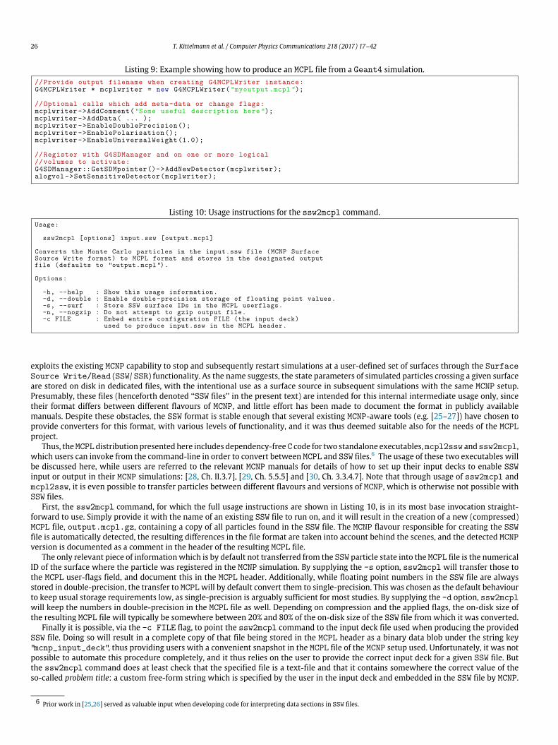
In Listing 9 is shown how the G4MCPLWriterwill typically be configured and attached to logical volume(s) of the geometry.
3.2. MCNP interface
Most users of MCNP are currently employing one of three distinct flavours: MCNPX [21,22], MCNP5 [23] or MCNP6 [24]. In the mosttypical mode of working with any of these software packages, users edit and launch MCNP through the use of text-based configuration files(so-called input decks), in order to set up details of the simulation including geometry, particle generation, and data extraction. The lattertypically results in the creation of data files containing simulation results, ready for subsequent analysis.
Although it would be conceivable towrite in-process FORTRAN-compatible MCPL hooks for MCNP, such an approachwould require usersto undertake some formof compilation and linking procedure. Thiswould likely impose a change inworkingmode for themajority of MCNPusers, in addition to possibly requiring a special license for source-level access to MCNP. Instead, the MCNP–MCPL interface presented here
26 T. Kittelmann et al. / Computer Physics Communications 218 (2017) 17–42
Listing 9: Example showing how to produce an MCPL file from a Geant4 simulation.//Provide output filename when creating G4MCPLWriter instance:G4MCPLWriter * mcplwriter = new G4MCPLWriter( " myoutput.mcpl " );
//Optional calls which add meta-data or change flags:mcplwriter ->AddComment( " Some useful description here " );mcplwriter ->AddData( ... );mcplwriter ->EnableDoublePrecision();mcplwriter ->EnablePolarisation();mcplwriter ->EnableUniversalWeight(1.0);
//Register with G4SDManager and on one or more logical//volumes to activate:G4SDManager::GetSDMpointer()->AddNewDetector(mcplwriter);alogvol->SetSensitiveDetector(mcplwriter);
Listing 10: Usage instructions for the ssw2mcpl command.Usage:
ssw2mcpl [options] input.ssw [output.mcpl]
Converts the Monte Carlo particles in the input.ssw file (MCNP SurfaceSource Write format) to MCPL format and stores in the designated outputfile (defaults to " output.mcpl ").
Options:
-h, --help : Show this usage information.-d, --double : Enable double-precision storage of floating point values.-s, --surf : Store SSW surface IDs in the MCPL userflags.-n, --nogzip : Do not attempt to gzip output file.-c FILE : Embed entire configuration FILE (the input deck)
used to produce input.ssw in the MCPL header.
exploits the existing MCNP capability to stop and subsequently restart simulations at a user-defined set of surfaces through the SurfaceSource Write/Read (SSW/ SSR) functionality. As the name suggests, the state parameters of simulated particles crossing a given surfaceare stored on disk in dedicated files, with the intentional use as a surface source in subsequent simulations with the same MCNP setup.Presumably, these files (henceforth denoted ‘‘SSW files’’ in the present text) are intended for this internal intermediate usage only, sincetheir format differs between different flavours of MCNP, and little effort has been made to document the format in publicly availablemanuals. Despite these obstacles, the SSW format is stable enough that several existing MCNP-aware tools (e.g. [25–27]) have chosen toprovide converters for this format, with various levels of functionality, and it was thus deemed suitable also for the needs of the MCPLproject.
Thus, theMCPLdistribution presented here includes dependency-freeC code for two standalone executables,mcpl2ssw andssw2mcpl,which users can invoke from the command-line in order to convert between MCPL and SSW files.6 The usage of these two executables willbe discussed here, while users are referred to the relevant MCNP manuals for details of how to set up their input decks to enable SSWinput or output in their MCNP simulations: [28, Ch. II.3.7], [29, Ch. 5.5.5] and [30, Ch. 3.3.4.7]. Note that through usage of ssw2mcpl andmcpl2ssw, it is even possible to transfer particles between different flavours and versions of MCNP, which is otherwise not possible withSSW files.
First, the ssw2mcpl command, for which the full usage instructions are shown in Listing 10, is in its most base invocation straight-forward to use. Simply provide it with the name of an existing SSW file to run on, and it will result in the creation of a new (compressed)MCPL file, output.mcpl.gz, containing a copy of all particles found in the SSW file. The MCNP flavour responsible for creating the SSWfile is automatically detected, the resulting differences in the file format are taken into account behind the scenes, and the detected MCNPversion is documented as a comment in the header of the resulting MCPL file.
The only relevant piece of informationwhich is by default not transferred from the SSW particle state into the MCPL file is the numericalID of the surface where the particle was registered in the MCNP simulation. By supplying the -s option, ssw2mcpl will transfer those tothe MCPL user-flags field, and document this in the MCPL header. Additionally, while floating point numbers in the SSW file are alwaysstored in double-precision, the transfer to MCPLwill by default convert them to single-precision. This was chosen as the default behaviourto keep usual storage requirements low, as single-precision is arguably sufficient for most studies. By supplying the -d option, ssw2mcplwill keep the numbers in double-precision in the MCPL file as well. Depending on compression and the applied flags, the on-disk size ofthe resulting MCPL file will typically be somewhere between 20% and 80% of the on-disk size of the SSW file from which it was converted.
Finally it is possible, via the -c FILE flag, to point the ssw2mcpl command to the input deck file used when producing the providedSSW file. Doing so will result in a complete copy of that file being stored in the MCPL header as a binary data blob under the string key"mcnp_input_deck", thus providing users with a convenient snapshot in the MCPL file of the MCNP setup used. Unfortunately, it was notpossible to automate this procedure completely, and it thus relies on the user to provide the correct input deck for a given SSW file. Butthe ssw2mcpl command does at least check that the specified file is a text-file and that it contains somewhere the correct value of theso-called problem title: a custom free-form string which is specified by the user in the input deck and embedded in the SSW file by MCNP.
6 Prior work in [25,26] served as valuable input when developing code for interpreting data sections in SSW files.

T. Kittelmann et al. / Computer Physics Communications 218 (2017) 17–42 27
Listing 11: Usage instructions for the mcpl2ssw command.Usage:
mcpl2ssw [options] <input.mcpl> <reference.ssw> [output.ssw]
Converts the Monte Carlo particles in the input MCPL file to SSW format(MCNP Surface Source Write) and stores the result in the designated outputfile (defaults to " output.ssw ").
In order to do so and get the details of the SSW format correct, the usermust also provide a reference SSW file from the same approximate setup(MCNP version, input deck...) where the new SSW file is to be used. Thereference SSW file can of course be very small, as only the file header isimportant (the new file essentially gets a copy of the header found in thereference file, except for certain fields related to number of particleswhose values are changed).
Finally, one must pay attention to the Surface ID assigned to theparticles in the resulting SSW file: Either the user specifies a globalone with -s<ID>, or it is assumed that the MCPL userflags field in theinput file is actually intended to become the Surface ID. Note that notall MCPL files have userflag fields and that valid Surface IDs areintegers in the range 1-999999.
Options:
-h, --help : Show this usage information.-s<ID> : All particles in the SSW file will get this surface ID.-l<LIMIT> : Limit the number of particles transferred to the SSW file
(defaults to 2147483647, the maximal SSW capacity).
The input deck embedded in a given MCPL file can later be inspected from the command line by invoking the command ‘‘mcpltool -bmcnp_input_deck <file.mcpl>’’.
Usage of the mcpl2ssw command, for which the full usage instructions are shown in Listing 11, is slightly more involved: in additionto an input MCPL file, the user must also supply a reference SSW file in a format suitable for the MCNP setup in which the resulting SSWfile is subsequently intended to be used as input. The need for this added complexity stems from the constraint that the SSW format ismerely intended as an internal format in which it is possible to stop and restart particles while remaining within a given setup of an MCNPsimulation – meaning at the very least that the MCNP version and the configuration of the geometrical surfaces involved in the SurfaceSource Write/Read procedure must be unchanged. Thus, for maximal robustness, the user must supply a reference SSW file which wasproduced by the setup in which the SSW file created with mcpl2ssw is to be used (it does not matter howmany particles the reference filecontains). What will actually happen is that in addition to the particle state data itself, the newly created SSW file will contain the exactsame header as the one in the reference SSW file, apart from the fields related to the number of particles in the file.
Additionally, the user must consider carefully which MCNP surface IDs the particles from the MCPL file should be associated with, oncetransferred to the SSW file. By default it will assume that the MCPL user-flags field contains exactly this ID, but more often than not, userswill have to specify a global surface ID for all of the particles through the -s<ID> command-line option for the mcpl2ssw command.
Finally, note that SSW files do not contain polarisation information, and any such polarisation information in the input MCPL file willconsequently be discarded in the translation. Likewise, in cases where the input MCPL file contains one or more particles whose type doesnot have a representation in the targeted flavour of MCNP, they will be ignored with suitable warnings.
3.3. McStas and McXtrace interfaces
Recent releases of the neutron ray tracing software package McStas [17,18] (version 2.3 and later) and its X-ray sibling packageMcXtrace [19] (version 1.4 and later) include MCPL-interfaces. Although McStas and McXtrace are two distinct software packages,they are implemented upon a common technological platform, McCode, and the discussions here will for simplicity use the term McCodewhere the instructions are otherwise identical for users of the two packages.
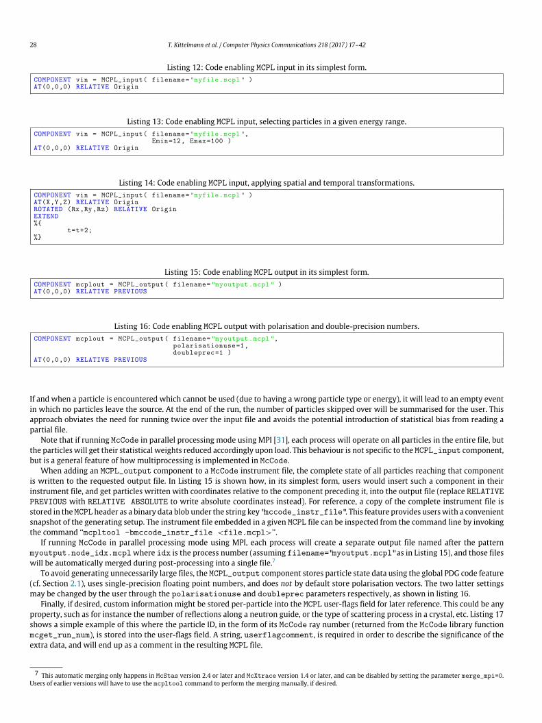
The particle model adopted in McCode is directly compatible with MCPL. In essence, apart from simple unit conversions, particles areread from or written to MCPL files at one or more predefined logical points defined in the McCode configuration files (so-called instrumentfiles). Specifically, two new components, MCPL_input and MCPL_output, are provided, which users can activate by adding entries atrelevant points in their instrument files as is usual when working with McCode.
First, when using the MCPL_input component, particles are directly read from an MCPL input file and injected into the simulation atthe desired point, thus playing the role of a source. In Listing 12 is shown how, in its simplest form, users would insert an MCPL_inputcomponent in their instrument file. Thiswill result in the MCPL file being read in its entirety, and all found neutrons (for McStas) or gammaparticles (for McXtrace) traced through the McCode simulation. Listing 13 indicates how the user can additionally impose an allowedenergy range when loading particles by supplying the Emin and Emax parameters. The units aremeV and keV respectively for McStas andMcXtrace. Thus, the code in Listing 13 would select 12–100meV neutrons in McStas and 12–100keV gammas in McXtrace. A particlefrom the MCPL file is injected at the position indicated by its MCPL coordinates relative to the position of the MCPL_input componentin the McCode instrument. Thus, a user can impose coordinate transformations by altering the positioning of MCPL_input as shown inListing 14, which would shift the initial position of the particles by (X, Y , Z) and rotate their initial velocities around the x, y and z axes(in that order) by respectively Rx, Ry and Rz degrees. Furthermore, Listing 14 shows a way to introduce a time shift of 2 s to all particles,using an EXTEND code block.
For technical reasons, the number of particles to be simulated in McCode must be fixed at initialisation time. Thus, the number ofparticles will be set to the total number of particles in the input file, as this is provided through the corresponding MCPL header field.
28 T. Kittelmann et al. / Computer Physics Communications 218 (2017) 17–42
Listing 12: Code enabling MCPL input in its simplest form.COMPONENT vin = MCPL_input( filename= " myfile.mcpl " )AT(0,0,0) RELATIVE Origin
Listing 13: Code enabling MCPL input, selecting particles in a given energy range.COMPONENT vin = MCPL_input( filename= " myfile.mcpl " ,
Emin=12, Emax=100 )AT(0,0,0) RELATIVE Origin
Listing 14: Code enabling MCPL input, applying spatial and temporal transformations.COMPONENT vin = MCPL_input( filename= " myfile.mcpl " )AT(X,Y,Z) RELATIVE OriginROTATED (Rx,Ry,Rz) RELATIVE OriginEXTEND%{
t=t+2;%}
Listing 15: Code enabling MCPL output in its simplest form.COMPONENT mcplout = MCPL_output( filename= " myoutput.mcpl " )AT(0,0,0) RELATIVE PREVIOUS
Listing 16: Code enabling MCPL output with polarisation and double-precision numbers.COMPONENT mcplout = MCPL_output( filename= " myoutput.mcpl " ,
polarisationuse=1,doubleprec=1 )
AT(0,0,0) RELATIVE PREVIOUS
If and when a particle is encountered which cannot be used (due to having a wrong particle type or energy), it will lead to an empty eventin which no particles leave the source. At the end of the run, the number of particles skipped over will be summarised for the user. Thisapproach obviates the need for running twice over the input file and avoids the potential introduction of statistical bias from reading apartial file.
Note that if running McCode in parallel processing mode using MPI [31], each process will operate on all particles in the entire file, butthe particles will get their statistical weights reduced accordingly upon load. This behaviour is not specific to the MCPL_input component,but is a general feature of how multiprocessing is implemented in McCode.
When adding an MCPL_output component to a McCode instrument file, the complete state of all particles reaching that componentis written to the requested output file. In Listing 15 is shown how, in its simplest form, users would insert such a component in theirinstrument file, and get particles written with coordinates relative to the component preceding it, into the output file (replace RELATIVEPREVIOUS with RELATIVE ABSOLUTE to write absolute coordinates instead). For reference, a copy of the complete instrument file isstored in the MCPL header as a binary data blob under the string key "mccode_instr_file". This feature provides userswith a convenientsnapshot of the generating setup. The instrument file embedded in a given MCPL file can be inspected from the command line by invokingthe command ‘‘mcpltool -bmccode_instr_file <file.mcpl>’’.
If running McCode in parallel processing mode using MPI, each process will create a separate output file named after the patternmyoutput.node_idx.mcplwhere idx is the process number (assuming filename="myoutput.mcpl" as in Listing 15), and those fileswill be automatically merged during post-processing into a single file.7
To avoid generating unnecessarily large files, the MCPL_output component stores particle state data using the global PDG code feature(cf. Section 2.1), uses single-precision floating point numbers, and does not by default store polarisation vectors. The two latter settingsmay be changed by the user through the polarisationuse and doubleprec parameters respectively, as shown in listing 16.
Finally, if desired, custom information might be stored per-particle into the MCPL user-flags field for later reference. This could be anyproperty, such as for instance the number of reflections along a neutron guide, or the type of scattering process in a crystal, etc. Listing 17shows a simple example of this where the particle ID, in the form of its McCode ray number (returned from the McCode library functionmcget_run_num), is stored into the user-flags field. A string, userflagcomment, is required in order to describe the significance of theextra data, and will end up as a comment in the resulting MCPL file.
7 This automatic merging only happens in McStas version 2.4 or later and McXtrace version 1.4 or later, and can be disabled by setting the parameter merge_mpi=0.Users of earlier versions will have to use the mcpltool command to perform the merging manually, if desired.

T. Kittelmann et al. / Computer Physics Communications 218 (2017) 17–42 29
Listing 17: Code enabling MCPL output with custom user-flags information./* some upstream component setting a variable (customvar) */COMPONENT some_comp = Some_Component( /* some parameters here */ )AT (0,0,0) ABSOLUTEEXTEND %{
customvar=(uint32_t) mcget_run_num();%}
/* MCPL output capturing customvar into MCPL user-flags */COMPONENT vout = MCPL_output( filename= " myoutput.mcpl " ,
userflag=customvar ,userflagcomment= " Particle Id " )
AT(0,0,0) RELATIVE PREVIOUS
4. Example scientific use cases
The possible uses for MCPL are envisioned to be many and varied, facilitating both straight-forward transfers of particle data betweendifferent simulations, as well as data reuse and cross-code comparisons. Actual scientific studies are already being performed with thehelp of MCPL, demonstrating the suitability of the format ‘‘in the field’’. By way of example, it will be discussed in the following how MCPLis used in two such ongoing studies.
4.1. Optimising the detectors for the LoKI instrument at ESS
The ongoing construction of the European Spallation Source (ESS) [11,12] has initiated significant development of novel neutronictechnologies in the past 5 years. The performance requirements for neutron instruments at the ESS, in particular those resulting from theunprecedented cold and thermal neutron brightness, are at or beyond the capabilities of detector technologies currently available [32].Additionally, shortage of 3He [33,34], uponwhich the vast majority of previous detectors were based, augments the need for developmentof new efficient and cost-effective detectors based on other isotopes with high neutronic conversion cross sections.
A typical approach to instrument design and optimisation at ESS involves the development of a McStas-based simulation ofthe instrument. Such a simulation includes an appropriate neutron source description and detailed models of the major instrumentcomponents, such as benders, neutron guides, chopper systems, collimators, sample environment and sample. See [35] for an introductionto the role of the various instrument components. Detector components in McStas are, however, typically not implemented with anydetailed modelling, and are simply registering all neutrons as they arrive. Thus, while the setup in McStas allows for an efficient andprecise optimisation of most of the instrument parameters, detailed detector optimisation studies must out of necessity be carried out ina separate simulation package, such as Geant4.
As the detector development progresses in parallel with the general instrument design, it is crucial to be able to optimise the detectorsetup for the exact instrument conditions under investigation in McStas. The MCPL format, along with the interfaces discussed inSections 3.1 and 3.3, facilitates this by allowing for easy transfer of neutron states from the McStas instrument simulation into Geant4simulations with detailed setups of proposed detector designs.
Technically, this is done by placing the MCPL_output component just after the relevant sample component in the McStas instrumentfile. Additionally, using the procedure for creation and storage of custom MCPL user-flags also discussed in Section 3.3, it is possible todifferentiate neutrons that scattered on the sample from thosewhich continued undisturbed, and to carry this information into theGeant4simulations. This information is needed to understand the impact of the direct beam on the low angle measurements, in order to studythe requirements for a so-called zero-angle detector.
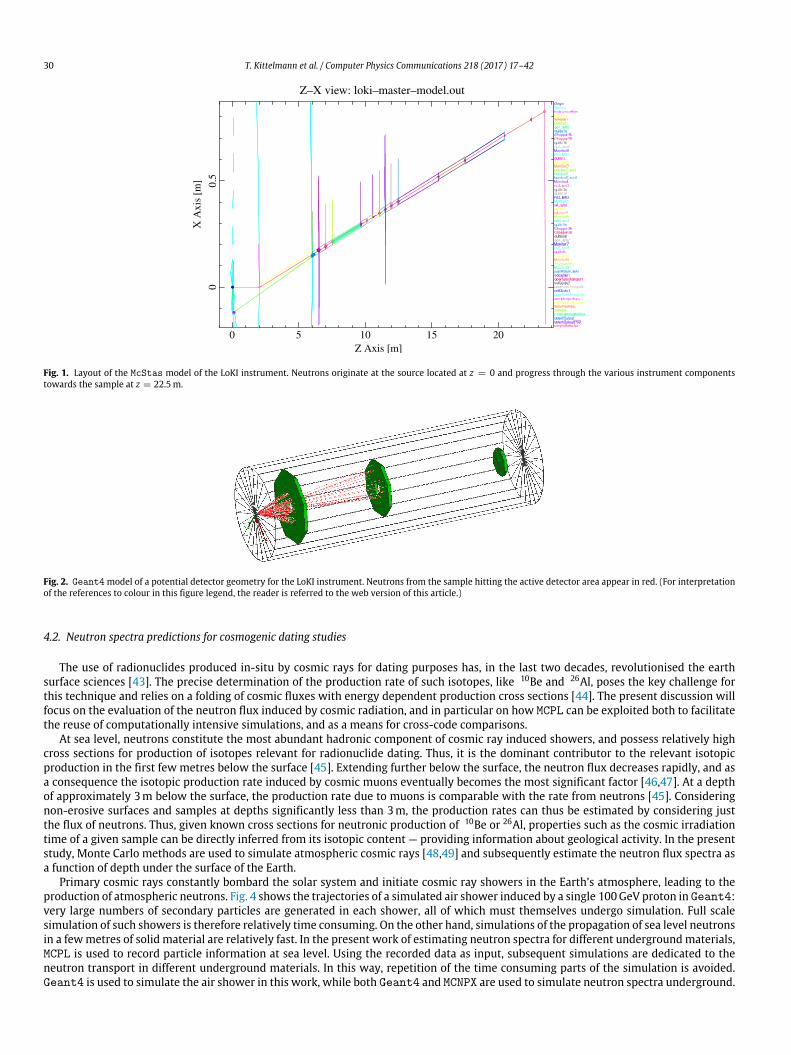
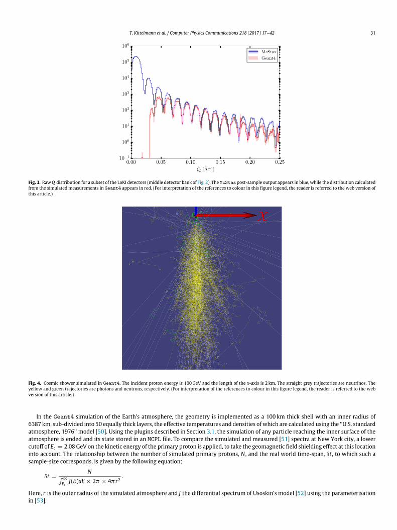
For example, in order to optimise the detector technology that the LoKI instrument [36–38]might adopt, a series of McStas simulationsof the instrument components and the interactions in realistic samples [39] are performed (see Fig. 1 for a view of the instrument inMcStas). The parameters of the instrument and the samples in the McStas model are chosen in such a way, that various aspects ofthe detector performance can be investigated, including rate capability and spatial resolution. The neutrons emerging from the sample inMcStas are then transferred via MCPL to the detector simulation in Geant4, where a detailed detector geometry and appropriatematerialsare implemented (see Fig. 2 for a visualisation of the Geant4model).
Neutrons traversing the detector geometry in Geant4 undergo interactions with thematerials they pass on their flight-path, accordingto the physics processes and respective cross sections available in the setup. Special attention is needed when configuring the Geant4physics modelling, to ensure that all processes relevant for neutron detection are taken into account and handled correctly. Specifically,the setup utilises the high-precision neutron models in Geant4 extended with [40], and is implemented in [10]. In the solid-converterbased detectors under consideration, a neutron absorption results in emission of charged products which then travel a certain rangeinside the detector and deposit energy in a counting gas. It is possible to extract position and time information from the energy depositionprofile and use these space–time coordinates for further analysis, in the same way that measurements in a real detector would be treated.This way it becomes possible to reproduce the distributions of observable quantities relevant for Small Angle Neutron Scattering (SANS)analysis [41,42].
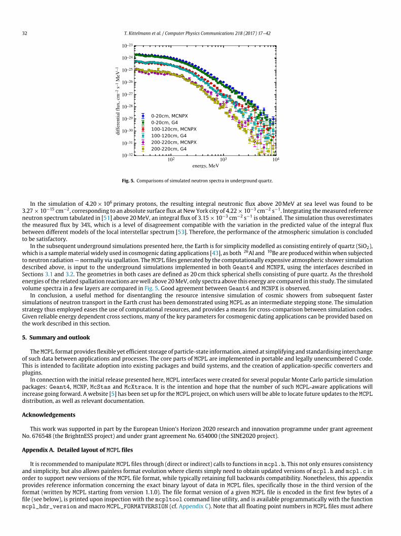
One such observable quantity is the Q distribution [35, Ch. 2.3.3], where Q is defined as the momentum change of the neutron as itscatters on the sample, divided by h̄: Q ≡ |∆p⃗|/h̄. Fig. 3 demonstrates such a distribution, based on the simulated output of the middledetector bank of LoKI (cf. Fig. 2), for a certain instrument setup — including a sample modelled as consisting of spheres with radii of 200Å.The raw Q distribution is calculated both based on the neutron states as they emerge from the sample in McStas, and from the simulatedmeasurements in Geant4. With such a procedure, resolution-smearing effects can be correctly attributed to their sources, geometricalacceptance and detector efficiency can be studied in detail, and the impact of engineering features such as dead space can be accuratelyconsidered.
30 T. Kittelmann et al. / Computer Physics Communications 218 (2017) 17–42
Fig. 1. Layout of the McStas model of the LoKI instrument. Neutrons originate at the source located at z = 0 and progress through the various instrument componentstowards the sample at z = 22.5m.
Fig. 2. Geant4model of a potential detector geometry for the LoKI instrument. Neutrons from the sample hitting the active detector area appear in red. (For interpretationof the references to colour in this figure legend, the reader is referred to the web version of this article.)
4.2. Neutron spectra predictions for cosmogenic dating studies
The use of radionuclides produced in-situ by cosmic rays for dating purposes has, in the last two decades, revolutionised the earthsurface sciences [43]. The precise determination of the production rate of such isotopes, like 10Be and 26Al, poses the key challenge forthis technique and relies on a folding of cosmic fluxes with energy dependent production cross sections [44]. The present discussion willfocus on the evaluation of the neutron flux induced by cosmic radiation, and in particular on how MCPL can be exploited both to facilitatethe reuse of computationally intensive simulations, and as a means for cross-code comparisons.
At sea level, neutrons constitute the most abundant hadronic component of cosmic ray induced showers, and possess relatively highcross sections for production of isotopes relevant for radionuclide dating. Thus, it is the dominant contributor to the relevant isotopicproduction in the first few metres below the surface [45]. Extending further below the surface, the neutron flux decreases rapidly, and asa consequence the isotopic production rate induced by cosmic muons eventually becomes the most significant factor [46,47]. At a depthof approximately 3m below the surface, the production rate due to muons is comparable with the rate from neutrons [45]. Consideringnon-erosive surfaces and samples at depths significantly less than 3m, the production rates can thus be estimated by considering justthe flux of neutrons. Thus, given known cross sections for neutronic production of 10Be or 26Al, properties such as the cosmic irradiationtime of a given sample can be directly inferred from its isotopic content — providing information about geological activity. In the presentstudy, Monte Carlo methods are used to simulate atmospheric cosmic rays [48,49] and subsequently estimate the neutron flux spectra asa function of depth under the surface of the Earth.
Primary cosmic rays constantly bombard the solar system and initiate cosmic ray showers in the Earth’s atmosphere, leading to theproduction of atmospheric neutrons. Fig. 4 shows the trajectories of a simulated air shower induced by a single 100GeV proton in Geant4:very large numbers of secondary particles are generated in each shower, all of which must themselves undergo simulation. Full scalesimulation of such showers is therefore relatively time consuming. On the other hand, simulations of the propagation of sea level neutronsin a fewmetres of solid material are relatively fast. In the present work of estimating neutron spectra for different undergroundmaterials,MCPL is used to record particle information at sea level. Using the recorded data as input, subsequent simulations are dedicated to theneutron transport in different underground materials. In this way, repetition of the time consuming parts of the simulation is avoided.Geant4 is used to simulate the air shower in this work, while both Geant4 and MCNPX are used to simulate neutron spectra underground.
T. Kittelmann et al. / Computer Physics Communications 218 (2017) 17–42 31
Fig. 3. RawQ distribution for a subset of the LoKI detectors (middle detector bank of Fig. 2). The McStas post-sample output appears in blue, while the distribution calculatedfrom the simulated measurements in Geant4 appears in red. (For interpretation of the references to colour in this figure legend, the reader is referred to the web version ofthis article.)
Fig. 4. Cosmic shower simulated in Geant4. The incident proton energy is 100GeV and the length of the x-axis is 2 km. The straight grey trajectories are neutrinos. Theyellow and green trajectories are photons and neutrons, respectively. (For interpretation of the references to colour in this figure legend, the reader is referred to the webversion of this article.)
In the Geant4 simulation of the Earth’s atmosphere, the geometry is implemented as a 100km thick shell with an inner radius of6387km, sub-divided into 50 equally thick layers, the effective temperatures and densities of which are calculated using the ‘‘U.S. standardatmosphere, 1976’’ model [50]. Using the plugins described in Section 3.1, the simulation of any particle reaching the inner surface of theatmosphere is ended and its state stored in an MCPL file. To compare the simulated and measured [51] spectra at New York city, a lowercutoff of Ec = 2.08 GeV on the kinetic energy of the primary proton is applied, to take the geomagnetic field shielding effect at this locationinto account. The relationship between the number of simulated primary protons, N , and the real world time-span, δt , to which such asample-size corresponds, is given by the following equation:
δt =N∫
∞
EcJ(E)dE × 2π × 4πr2
.
Here, r is the outer radius of the simulated atmosphere and J the differential spectrum of Usoskin’s model [52] using the parameterisationin [53].
32 T. Kittelmann et al. / Computer Physics Communications 218 (2017) 17–42
Fig. 5. Comparisons of simulated neutron spectra in underground quartz.
In the simulation of 4.20×10⁶ primary protons, the resulting integral neutronic flux above 20MeV at sea level was found to be3.27×10−15 cm−2, corresponding to an absolute surface flux at NewYork city of 4.22×10⁻³ cm−2 s−1. Integrating themeasured referenceneutron spectrum tabulated in [51] above 20MeV, an integral flux of 3.15×10⁻³ cm−2 s−1 is obtained. The simulation thus overestimatesthe measured flux by 34%, which is a level of disagreement compatible with the variation in the predicted value of the integral fluxbetween different models of the local interstellar spectrum [53]. Therefore, the performance of the atmospheric simulation is concludedto be satisfactory.
In the subsequent underground simulations presented here, the Earth is for simplicity modelled as consisting entirely of quartz (SiO2),which is a samplematerial widely used in cosmogenic dating applications [43], as both 26Al and 10Be are producedwithinwhen subjectedto neutron radiation—normally via spallation. The MCPL files generated by the computationally expensive atmospheric shower simulationdescribed above, is input to the underground simulations implemented in both Geant4 and MCNPX, using the interfaces described inSections 3.1 and 3.2. The geometries in both cases are defined as 20 cm thick spherical shells consisting of pure quartz. As the thresholdenergies of the related spallation reactions arewell above 20MeV, only spectra above this energy are compared in this study. The simulatedvolume spectra in a few layers are compared in Fig. 5. Good agreement between Geant4 and MCNPX is observed.
In conclusion, a useful method for disentangling the resource intensive simulation of cosmic showers from subsequent fastersimulations of neutron transport in the Earth crust has been demonstrated using MCPL as an intermediate stepping stone. The simulationstrategy thus employed eases the use of computational resources, and provides a means for cross-comparison between simulation codes.Given reliable energy dependent cross sections, many of the key parameters for cosmogenic dating applications can be provided based onthe work described in this section.
5. Summary and outlook
TheMCPL format provides flexible yet efficient storage of particle-state information, aimed at simplifying and standardising interchangeof such data between applications and processes. The core parts of MCPL are implemented in portable and legally unencumbered C code.This is intended to facilitate adoption into existing packages and build systems, and the creation of application-specific converters andplugins.
In connection with the initial release presented here, MCPL interfaces were created for several popular Monte Carlo particle simulationpackages: Geant4, MCNP, McStas and McXtrace. It is the intention and hope that the number of such MCPL-aware applications willincrease going forward. A website [5] has been set up for the MCPL project, on which users will be able to locate future updates to the MCPLdistribution, as well as relevant documentation.
Acknowledgements
This work was supported in part by the European Union’s Horizon 2020 research and innovation programme under grant agreementNo. 676548 (the BrightnESS project) and under grant agreement No. 654000 (the SINE2020 project).
Appendix A. Detailed layout of MCPL files
It is recommended to manipulate MCPL files through (direct or indirect) calls to functions in mcpl.h. This not only ensures consistencyand simplicity, but also allows painless format evolution where clients simply need to obtain updated versions of mcpl.h and mcpl.c inorder to support new versions of the MCPL file format, while typically retaining full backwards compatibility. Nonetheless, this appendixprovides reference information concerning the exact binary layout of data in MCPL files, specifically those in the third version of theformat (written by MCPL starting from version 1.1.0). The file format version of a given MCPL file is encoded in the first few bytes of afile (see below), is printed upon inspection with the mcpltool command line utility, and is available programmatically with the functionmcpl_hdr_version and macro MCPL_FORMATVERSION (cf. Appendix C). Note that all floating point numbers in MCPL files must adhere

T. Kittelmann et al. / Computer Physics Communications 218 (2017) 17–42 33
Table A.1Detailed layout of the first part of the header section of an MCPL file.
Header layout (first part)
Position Size Type Description
0 4B – Magic number identifying file as an MCPL file. Value is always0x4d43504c (‘‘MCPL’’ in ASCII).
4 3B – File format version encoded as 3 digit zero-prefixed ASCII number(e.g. ‘‘003’’).
7 1B – Endianness of numbers in file, 0x4c (ASCII ‘‘L’’) for little or 0x42(ASCII ‘‘B’’) for big.
8 8B UINT64 Number of particles in file.16 4B UINT32 Number of custom comments in file, NCMTS.20 4B UINT32 Number of custom binary data blobs in file, NBLOBS.24 4B UINT32 Flag signifying whether user-flags are enabled (0x1) or disabled (0x0).28 4B UINT32 Flag signifying whether polarisation vectors are enabled (0x1) or
disabled (0x0).32 4B UINT32 Flag signifying whether floating point numbers in the particle data
section are in double- (0x0) or single-precision (0x1).36 4B INT32 Value of universal PDG code. A value of 0x0 means that particles in the
file all have their own PDG code field.40 4B UINT32 Data length per particle (redundant information, as it can be inferred
from the other flags and values).44 4B UINT32 Flag signifying whether a universal weight is present in the header
(0x1) or if particles in the file all have their own weight field (0x0).
Table A.2Detailed layout of the second part of the header section of an MCPL file. The presence and count of entries here dependson values found in the first part of the header section (cf. Table A.1).
Header layout (second part)
Size Type Description
0B or 8B FP64 Value of the universal weight, if enabled.4B+ DATA ARRAY Data is a string holding the user provided ‘‘Source name’’. This is
always present, but might be empty.NCMTS × 4B+ DATA ARRAYS One data array for each comment, holding the user provided
comments as strings.NBLOBS × 4B+ DATA ARRAYS One data array for each binary data blob, holding the user provided
blob keys as strings.NBLOBS × 4B+ DATA ARRAYS One data array for each binary data blob, holding the actual binary data
(in the same order as the blob keys).
to the IEEE-754 floating point standard [7] for single- (32 bit) or double-precision (64 bit) as relevant. All signed integers in the file mustfollow the ubiquitous ‘‘two’s complement’’ representation.
The first 48 bytes of an MCPL file follow a fixed layout, as indicated in Table A.1, providing flags and values needed to read and interpretboth the particle data section and the remainder of the header section. Note that abbreviations used for type information in tables inthis appendix are UINT32 and UINT64 for 32 and 64 bit unsigned integers respectively, INT32 for 32 bit signed integers and FP64 fordouble-precision 64 bit floating point numbers.
The layout of the second part of the header section is indicated in Table A.2, and includes both optional and repeated entries and entrieswith flexible length. Entries with type listed as ‘‘DATA ARRAY’’ are arbitrary length byte-arrays in which the first four bytes are unsigned32 bit integers indicating the byte length of the data payload which follows just after. Note that strings are stored like any other data, withthe only twist being that terminating NULL characters are not stored.
Next, after the header section, the remainder of the file consists of the particle data section. It contains one entry for each particle in thefile, with detailed layout of each as indicated in Table A.3. Here, FP is either single- (32 bit) or double-precision (64 bit) numbers, dependingon the relevant flag in the file header. Concerning the 3 floating point numbers used to represent the packed direction vector and kineticenergy, the scheme is as discussed in Appendix B: the first and second of the 3 floating point numbers are respectively FP1 and FP2 fromTable B.1, while the third is a number whose magnitude is given by the particle’s kinetic energy and whose sign bit is used to store the lastbit of information needed for the direction vector, indicated in the ‘‘+1 bit’’ column of Table B.1. Specifically, the sign bit is set when thenumber indicated in the ‘‘+1 bit’’ column is negative.
Appendix B. Unit vector packing
From a purely mathematical perspective, it is trivial to ‘‘pack’’ unit vectors specified in three-dimensional Cartesian coordinates into atwo-dimensional coordinate space, and it can for instance be achieved by the standard transformation between Cartesian and Sphericalcoordinates. However, when considering floating point numbers rather than the ideal mathematical abstraction of the complete set ofreal numbers, issues of numerical imprecision during the packing and subsequent unpacking transformations become crucial. Where itmatters, the discussion in this appendix will, like the MCPL format in general, assume floating point numbers to adhere to the relevantIEEE floating point standard [7].
A few different packing algorithms will be compared in this appendix. First of all, the spherical transformation between Cartesian unitvectors (ux, uy, uz) and spherical coordinates (θ, φ) is investigated, using the C math library functions acos, atan2, sin and cos in anobviousmannerwhen implementing the transformations. In addition to the significant computational overhead involvedwhen evaluating

34 T. Kittelmann et al. / Computer Physics Communications 218 (2017) 17–42
Table A.3Detailed layout of the data associated with each particle in an MCPL file.
Particle data layout
Presence Count & type Description
OPTIONAL 3 × FP Polarisation vector (if enabled in file).ALWAYS 3 × FP Position vectorALWAYS 3 × FP Packed direction vector and kinetic energy.ALWAYS 1 × FP Time.OPTIONAL 1 × FP Weight (if file does not have universal weight).OPTIONAL 1 × INT32 PDG code (if file does not have universal PDG code).OPTIONAL 1 × UINT32 User-flags (if enabled in file).
Table B.1Breakdown of the Adaptive Projection Packing method, in which a unit vector, (ux, uy, uz ) is stored into two floatingpoint numbers, FP1 and FP2, and one extra bit of information.
Adaptive Projection Packing
Scenario FP1 FP2 +1 bit Packed signature
|ux| largest 1/uz uy sign(ux) |FP1| > 1, |FP2| < 1|uy| largest ux 1/uz sign(uy) |FP1| < 1, |FP2| > 1|uz | largest ux uy sign(uz ) |FP1| < 1, |FP2| < 1
trigonometric functions, numerical uncertainties also tend to blow up when a Cartesian coordinate is very small. For instance, considera unit vector with uz = ϵ for some |ϵ| ≪ 1. Then, θ = arccos(ϵ) which is to lowest order equal to π/2 − ϵ, a subtraction which out ofnecessity will cause a loss of precision when it is stored as a floating point number: if ϵ is N orders of magnitude smaller than π/2, thenthe stored result will be insensitive to the N least significant digits of information in the storage of ϵ. The calculation of φ suffers fromsimilar problems.
The next packing algorithm to be considered is what will be denoted the Static Projection method in the following. It represents thestraight-forward and widespread solution of storing two Cartesian components, ux and uy, directly and recovering the magnitude of thethird by the expression |uz | =
√1 − u2
x − u2y . This method, which incidentally is the one used internally in the SSW files produced by MCNP
(cf. Section 3.2), requires a single bit of additional storage to be available, in order to recover the sign of uz as well as its magnitude. Thisrequirement of an extra bit of storage is seen in several packing schemes and is not necessarily a problem, as will be discussed later. Whatis problematic, however, is that the calculation of
√1 − u2
x − u2y will result in large numerical uncertainties when the magnitude of uz is
small, as it implies the subtraction of large and nearly equal quantities and a resulting loss of significant digits in the result.Finally, inspired by a recent survey of unit vector packing techniques [54], a packing scheme using a so-called Octahedral Projection [55]
was also investigated. It is a variant of the Static Projection method in which the original point on the unit sphere is first projected ontoan octahedral surface before the resulting x and y coordinates are stored. Thus, the stored variables are (ox, oy) = (ux/n, uy/n) wheren = |ux| + |uy| + |uz |. Unpacking proceeds by first recovering the point on the octahedron as (ox, oy, 1 − |ox| − |oy|), and then projectingback out to the unit sphere with a simple normalisation, requiring the evaluation of a square root. Although the algorithm has improvedperformance over the methods already discussed, it once again suffers from numerical precision issues when applied to certain unitvectors. Consider for instance the unit vector (
√1 − ϵ2, 0, ϵ) for a very small but positive epsilon. Packing will result in oy = 0 and
ox = 1/(√1 − ϵ2 + ϵ) ≈ 1 − ϵ, storage of which discards the N least significant digits of ϵ, when ϵ is N orders of magnitude smaller than
unity. Finally, it should be mentioned that like the Static Projection method, the Octahedral Projection method also needs the sign of uzstored in a bit elsewhere. The present discussion thus ignores the method described in [54,55] of encoding the sign of uz by folding (ox, oy)into a separate part of the plane when uz < 0, as this operation introduces additional numerical imprecision and an undesired asymmetryinto the algorithm.
Although the three pre-existing packing methods discussed so far all represent potentially useful approaches to unit vector packingdepending on the particular needs of a given use-case, they were nonetheless deemed undesirable for a general purpose scientific formatlike MCPL. This is because MCPL is intended for usage in a wide variety of simulation scenarios, including those where some componentsof the directional unit vectors of stored particles could be truly minuscule but non-zero in magnitude. In order to better fulfil therequirements, a new unit vector packing algorithm was devised for MCPL. It is tentatively named Adaptive Projection Packing, and will bepresented in the following. The algorithm is based upon the simple observation that although the Static Projectionmethod has issueswhen|uz | ≪ 1, it provides very precise results when uz is the component with the largest magnitude. Thus, rather than always storing ux and uy,performance can be significantly improved by letting the packing algorithm select the two components with the smallest magnitudes andstore those. That leaves the issue that the unpacking algorithmmust be able to recognise which components were stored. The solution tothat is based upon the fact that all three components can have at most unit magnitude, and that |uz | ≤ 1/
√2 whenever it must be stored,
implying that 1/uz will have amagnitude larger than 1. Thus, by storing 1/uz in place of the one of ux and uy which is greater inmagnitude,the unpacking algorithm can easily tell which components are stored in which of the two packed numbers, merely by looking at how theirmagnitudes compare to unity (the code should obviously store the floating point representation of∞when uz = 0). The resulting encodingscheme is summarised in Table B.1: one of three storage scenarios is picked by the packing code, depending on themagnitudes of the threeunit vector components. The unique packed signature of each scenario, listed in the last column, enables them to be easily distinguishedby unpacking code. Although obviously more complicated than the Static Projection method, the added computational cost of using theAdaptive Projection method is at most a few branches and a division, which is found in the context of MCPL to be comparable to the costof the Octahedral Projection method and much faster than the Spherical coordinate method due to the expensive trigonometric functioncalls. In any case, the overhead is found to be insignificant given the intended usage in MCPL.

T. Kittelmann et al. / Computer Physics Communications 218 (2017) 17–42 35
Fig. B.1. Average packing precision of the considered unit vector packingmethods, as discussed in the text, for both double-precision (64 bit, full curves) and single-precision(32 bit, dashed opaque curves). The Adaptive Projection (blue, green) and No packing (black) curves are almost coinciding.
As indicated in Table B.1, the issue of needing one extra bit of storage space to hold the sign of the component which was projectedaway, has naturally been inherited from the Static Projectionmethod. Although finding anunusedbit could certainly present a challenge forsome applications of unit vector packing, it is not actually an issue for the MCPL format where an extra bit of information can be encodedinto the sign of the floating point number otherwise used to store the kinetic energy of the particle (cf. Table 2). This bit is otherwiseunused, since kinetic energy is a non-negative quantity by definition, and is available for usage even if particle states are specified witha kinetic energy of exactly zero. The latter follows from the IEEE floating point standard [7], which ensures availability of the sign biteven for zero (i.e. it provides a signed zero floating point implementation with distinct bit patterns for −0 and +0). Although it is thusnot needed for MCPL, it should be noted for completeness that it is straight-forward to implement a variant of the Adaptive Projectionmethodwhich simply allocates the ‘‘extra’’ bit of storage internally in one of the two resulting floating point numbers. This can be achievedby encoding the information into the least significant bit of the significand of either FP1 or FP2, thus sacrificing a small – but hopefullyinconsequential – amount of precision in the process.
In order to compare the performance of the considered packing algorithms quantitatively, the packing precision when a unit vectoru is transformed by the packing and unpacking into up is defined in the following. First, the packing precision of a single component,i ∈ {x, y, z}, is defined as δi ≡ min(1, |up
i /ui| − 1), except when ui = 0 in which case it is defined to be 0 if upi = ui, and 1 otherwise. The
packing precision for the entire vector is then defined as being the worst precision of any component, δ ≡ maxi δi. The resulting valueswill all lie in the unit interval and if for instance δ = 10−16, the packing algorithm in question can be said to have preserved the vectorwith at least 16 significant digits in all components. The reason for not picking a somewhat simpler figure of merit, such as the angularseparation between u and up, is that it would be insensitive to components which are very small in magnitude.
To be able to provide meaningful results for all considered packing methods, the analysis presented in the following was carriedout using software [56] capable of arbitrary precision floating-point arithmetic. Additionally it should be noted that, as the focus of thepresent analysis is on precision and storage consumption for a format like MCPL, the algorithms packing numbers into single-precision(32 bit) floating point storage are actually implemented using double-precision (64 bit) floating point code for all intermediate calculations.For other particular use-cases, such as graphics rendering with surface normals on a particular GPU, one could of course imagine alsoimplementing the packing code itself using single-precision everywhere.
Motivated by the fact that the considered packingmethods all have particular issues or strategieswhen uz is small inmagnitude, Fig. B.1illustrates their performance when applied to vectors with specific (possibly tiny) values of uz . For each given value of uz , a test set of 104
unit vectors is formed by sampling an azimuthal angle φ uniformly in [0, 2π ), and letting (ux, uy) =√1 − u2
z · (cosφ, sinφ). Each packingmethod is then applied to the test set, and the average value of the resulting packing precisions is plotted. The plot clearly confirmsthat while the Octahedral Projection method outperforms the Spherical coordinate and Static Projection methods, they all degrade inperformance as the magnitude of uz tends to zero. This is qualitatively different from the Adaptive Projection method, which showsconstant performance over the entire range, at a level which is practically indistinguishable from the case of not using any packing —i.e. storing the Cartesian coordinates directly into 3 dedicated floating point numbers. Note that for clarity the plot is only shown herefor positive uz larger than 10−20, but it was verified in a full analysis that, as expected, the flat level of the Adaptive Projection curves isindependent of the sign of uz , and continues unchanged over the entire dynamic range of normalised floating point numbers, down toabout 10−38 and 10−308 respectively for single- and double-precision.
As a natural figure of merit, Table B.2 shows the average packing precision of the considered methods when applied to a sample of 108
unit vectors sampled at random from an isotropic distribution. Although all methods provide some level of precision, it is clear that onlyAdaptive Projection Packing provides performance comparable to not using packing at all. In fact, for single-precision storage, AdaptiveProjection Packing in the 2FP+1bit variant relevant for MCPL, even seems to be outperforming the case of not using any packing. Thissomewhat counter-intuitive result is understood to arise from the fact that the unpacking code is implemented in full double-precision,
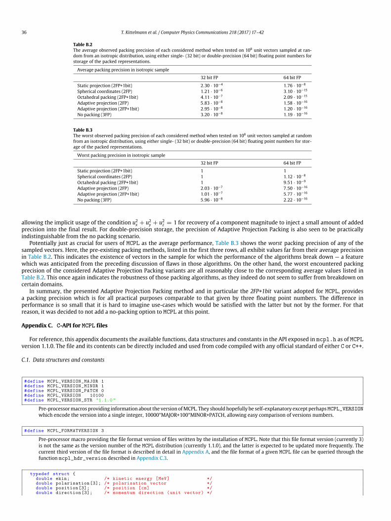
36 T. Kittelmann et al. / Computer Physics Communications 218 (2017) 17–42
Table B.2The average observed packing precision of each considered method when tested on 108 unit vectors sampled at ran-dom from an isotropic distribution, using either single- (32 bit) or double-precision (64 bit) floating point numbers forstorage of the packed representations.
Average packing precision in isotropic sample
32 bit FP 64 bit FP
Static projection (2FP+1bit) 2.30 · 10−4 1.76 · 10−8
Spherical coordinates (2FP) 1.21 · 10−6 3.10 · 10−15
Octahedral packing (2FP+1bit) 4.11 · 10−7 2.09 · 10−15
Adaptive projection (2FP) 5.83 · 10−8 1.58 · 10−16
Adaptive projection (2FP+1bit) 2.95 · 10−8 1.20 · 10−16
No packing (3FP) 3.20 · 10−8 1.19 · 10−16
Table B.3The worst observed packing precision of each considered method when tested on 108 unit vectors sampled at randomfrom an isotropic distribution, using either single- (32 bit) or double-precision (64 bit) floating point numbers for stor-age of the packed representations.
Worst packing precision in isotropic sample
32 bit FP 64 bit FP
Static projection (2FP+1bit) 1 1Spherical coordinates (2FP) 1 1.12 · 10−8
Octahedral packing (2FP+1bit) 1 9.51 · 10−9
Adaptive projection (2FP) 2.03 · 10−7 7.50 · 10−16
Adaptive projection (2FP+1bit) 1.01 · 10−7 5.77 · 10−16
No packing (3FP) 5.96 · 10−8 2.22 · 10−16
allowing the implicit usage of the condition u2x + u2
y + u2z = 1 for recovery of a component magnitude to inject a small amount of added
precision into the final result. For double-precision storage, the precision of Adaptive Projection Packing is also seen to be practicallyindistinguishable from the no packing scenario.
Potentially just as crucial for users of MCPL as the average performance, Table B.3 shows the worst packing precision of any of thesampled vectors. Here, the pre-existing packing methods, listed in the first three rows, all exhibit values far from their average precisionin Table B.2. This indicates the existence of vectors in the sample for which the performance of the algorithms break down — a featurewhich was anticipated from the preceding discussion of flaws in those algorithms. On the other hand, the worst encountered packingprecision of the considered Adaptive Projection Packing variants are all reasonably close to the corresponding average values listed inTable B.2. This once again indicates the robustness of those packing algorithms, as they indeed do not seem to suffer from breakdown oncertain domains.
In summary, the presented Adaptive Projection Packing method and in particular the 2FP+1bit variant adopted for MCPL, providesa packing precision which is for all practical purposes comparable to that given by three floating point numbers. The difference inperformance is so small that it is hard to imagine use-cases which would be satisfied with the latter but not by the former. For thatreason, it was decided to not add a no-packing option to MCPL at this point.
Appendix C. C-API for MCPL files
For reference, this appendix documents the available functions, data structures and constants in the API exposed in mcpl.h as of MCPLversion 1.1.0. The file and its contents can be directly included and used from code compiled with any official standard of either C or C++.
C.1. Data structures and constants
#define MCPL_VERSION_MAJOR 1#define MCPL_VERSION_MINOR 1#define MCPL_VERSION_PATCH 0#define MCPL_VERSION 10100#define MCPL_VERSION_STR " 1.1.0 "
Pre-processormacros providing information about the version ofMCPL. They should hopefully be self-explanatory except perhapsMCPL_VERSIONwhich encode the version into a single integer, 10000*MAJOR+100*MINOR+PATCH, allowing easy comparison of versions numbers.
#define MCPL_FORMATVERSION 3
Pre-processor macro providing the file format version of files written by the installation of MCPL. Note that this file format version (currently 3)is not the same as the version number of the MCPL distribution (currently 1.1.0), and the latter is expected to be updated more frequently. Thecurrent third version of the file format is described in detail in Appendix A, and the file format of a given MCPL file can be queried through thefunction mcpl_hdr_version described in Appendix C.3.
typedef struct {double ekin; /* kinetic energy [MeV] */double polarisation[3]; /* polarisation vector */double position[3]; /* position [cm] */double direction[3]; /* momentum direction (unit vector) */
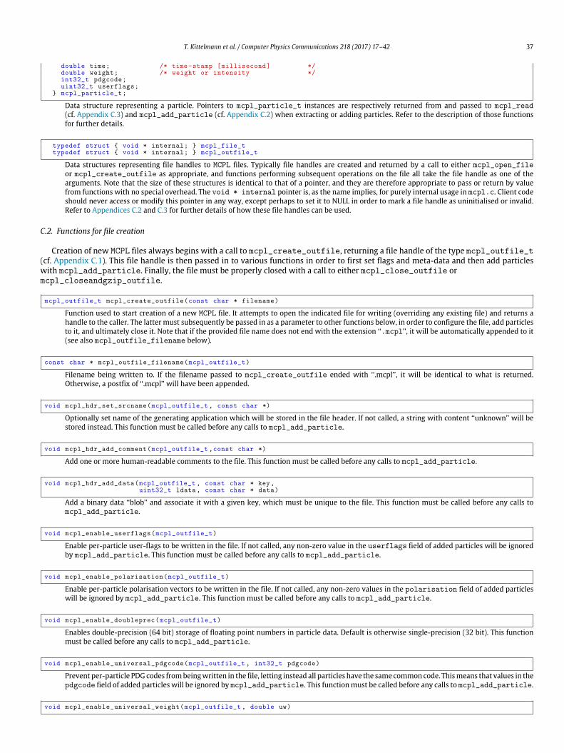
T. Kittelmann et al. / Computer Physics Communications 218 (2017) 17–42 37
double time; /* time-stamp [millisecond] */double weight; /* weight or intensity */int32_t pdgcode;uint32_t userflags;
} mcpl_particle_t;
Data structure representing a particle. Pointers to mcpl_particle_t instances are respectively returned from and passed to mcpl_read(cf. Appendix C.3) and mcpl_add_particle (cf. Appendix C.2) when extracting or adding particles. Refer to the description of those functionsfor further details.
typedef struct { void * internal; } mcpl_file_ttypedef struct { void * internal; } mcpl_outfile_t
Data structures representing file handles to MCPL files. Typically file handles are created and returned by a call to either mcpl_open_fileor mcpl_create_outfile as appropriate, and functions performing subsequent operations on the file all take the file handle as one of thearguments. Note that the size of these structures is identical to that of a pointer, and they are therefore appropriate to pass or return by valuefrom functions with no special overhead. The void * internal pointer is, as the name implies, for purely internal usage in mcpl.c. Client codeshould never access or modify this pointer in any way, except perhaps to set it to NULL in order to mark a file handle as uninitialised or invalid.Refer to Appendices C.2 and C.3 for further details of how these file handles can be used.
C.2. Functions for file creation
Creation of new MCPL files always begins with a call to mcpl_create_outfile, returning a file handle of the type mcpl_outfile_t(cf. Appendix C.1). This file handle is then passed in to various functions in order to first set flags and meta-data and then add particleswith mcpl_add_particle. Finally, the file must be properly closed with a call to either mcpl_close_outfile ormcpl_closeandgzip_outfile.
mcpl_outfile_t mcpl_create_outfile(const char * filename)
Function used to start creation of a new MCPL file. It attempts to open the indicated file for writing (overriding any existing file) and returns ahandle to the caller. The latter must subsequently be passed in as a parameter to other functions below, in order to configure the file, add particlesto it, and ultimately close it. Note that if the provided file name does not end with the extension ‘‘.mcpl’’, it will be automatically appended to it(see also mcpl_outfile_filename below).
const char * mcpl_outfile_filename(mcpl_outfile_t)
Filename being written to. If the filename passed to mcpl_create_outfile ended with ‘‘.mcpl’’, it will be identical to what is returned.Otherwise, a postfix of ‘‘.mcpl’’ will have been appended.
void mcpl_hdr_set_srcname(mcpl_outfile_t , const char *)
Optionally set name of the generating application which will be stored in the file header. If not called, a string with content ‘‘unknown’’ will bestored instead. This function must be called before any calls to mcpl_add_particle.
void mcpl_hdr_add_comment(mcpl_outfile_t ,const char *)
Add one or more human-readable comments to the file. This function must be called before any calls to mcpl_add_particle.
void mcpl_hdr_add_data(mcpl_outfile_t , const char * key,uint32_t ldata, const char * data)
Add a binary data ‘‘blob’’ and associate it with a given key, which must be unique to the file. This function must be called before any calls tomcpl_add_particle.
void mcpl_enable_userflags(mcpl_outfile_t)
Enable per-particle user-flags to be written in the file. If not called, any non-zero value in the userflags field of added particles will be ignoredby mcpl_add_particle. This function must be called before any calls to mcpl_add_particle.
void mcpl_enable_polarisation(mcpl_outfile_t)
Enable per-particle polarisation vectors to be written in the file. If not called, any non-zero values in the polarisation field of added particleswill be ignored by mcpl_add_particle. This function must be called before any calls to mcpl_add_particle.
void mcpl_enable_doubleprec(mcpl_outfile_t)
Enables double-precision (64 bit) storage of floating point numbers in particle data. Default is otherwise single-precision (32 bit). This functionmust be called before any calls to mcpl_add_particle.
void mcpl_enable_universal_pdgcode(mcpl_outfile_t , int32_t pdgcode)
Prevent per-particle PDG codes frombeingwritten in the file, letting instead all particles have the same common code. Thismeans that values in thepdgcode field of added particles will be ignored by mcpl_add_particle. This functionmust be called before any calls to mcpl_add_particle.
void mcpl_enable_universal_weight(mcpl_outfile_t , double uw)
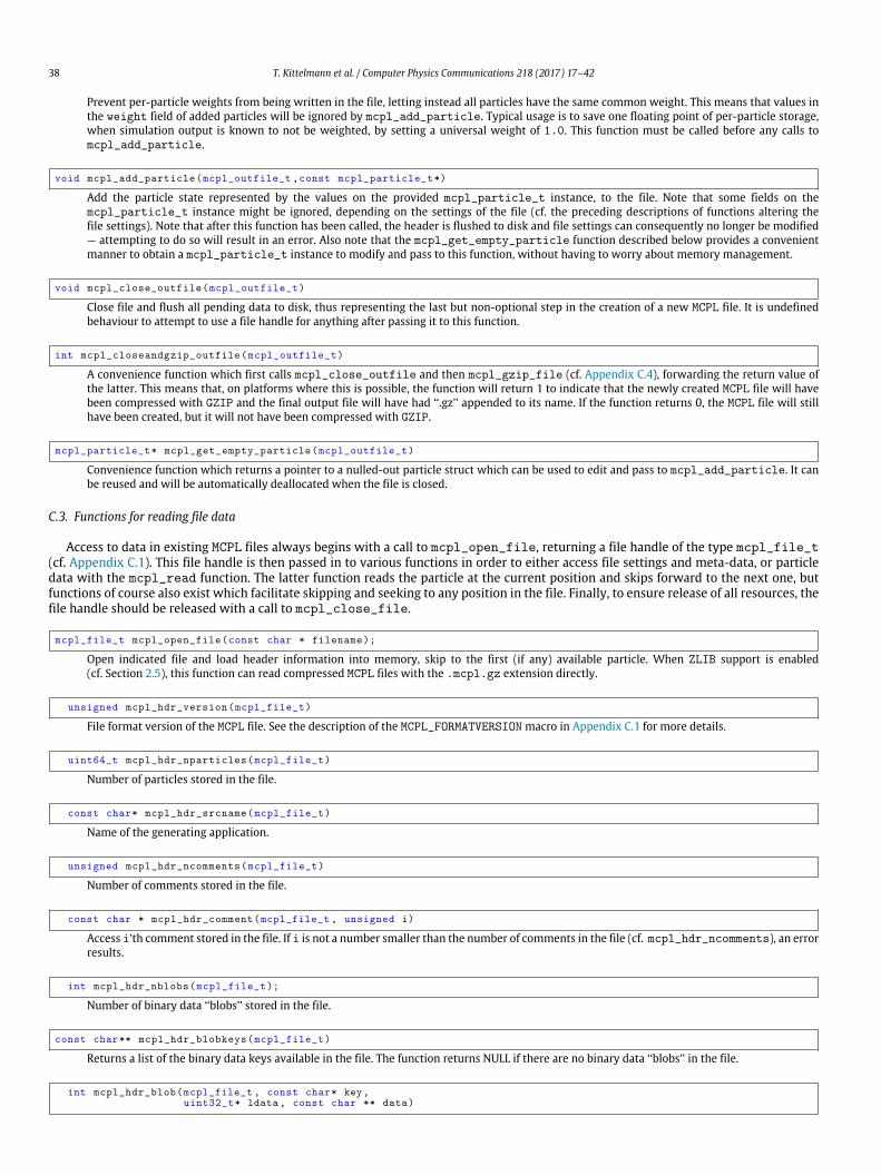
38 T. Kittelmann et al. / Computer Physics Communications 218 (2017) 17–42
Prevent per-particle weights from being written in the file, letting instead all particles have the same common weight. This means that values inthe weight field of added particles will be ignored by mcpl_add_particle. Typical usage is to save one floating point of per-particle storage,when simulation output is known to not be weighted, by setting a universal weight of 1.0. This function must be called before any calls tomcpl_add_particle.
void mcpl_add_particle(mcpl_outfile_t ,const mcpl_particle_t*)
Add the particle state represented by the values on the provided mcpl_particle_t instance, to the file. Note that some fields on themcpl_particle_t instance might be ignored, depending on the settings of the file (cf. the preceding descriptions of functions altering thefile settings). Note that after this function has been called, the header is flushed to disk and file settings can consequently no longer be modified— attempting to do so will result in an error. Also note that the mcpl_get_empty_particle function described below provides a convenientmanner to obtain a mcpl_particle_t instance to modify and pass to this function, without having to worry about memory management.
void mcpl_close_outfile(mcpl_outfile_t)
Close file and flush all pending data to disk, thus representing the last but non-optional step in the creation of a new MCPL file. It is undefinedbehaviour to attempt to use a file handle for anything after passing it to this function.
int mcpl_closeandgzip_outfile(mcpl_outfile_t)
A convenience function which first calls mcpl_close_outfile and then mcpl_gzip_file (cf. Appendix C.4), forwarding the return value ofthe latter. This means that, on platforms where this is possible, the function will return 1 to indicate that the newly created MCPL file will havebeen compressed with GZIP and the final output file will have had ‘‘.gz’’ appended to its name. If the function returns 0, the MCPL file will stillhave been created, but it will not have been compressed with GZIP.
mcpl_particle_t* mcpl_get_empty_particle(mcpl_outfile_t)
Convenience function which returns a pointer to a nulled-out particle struct which can be used to edit and pass to mcpl_add_particle. It canbe reused and will be automatically deallocated when the file is closed.
C.3. Functions for reading file data
Access to data in existing MCPL files always begins with a call to mcpl_open_file, returning a file handle of the type mcpl_file_t(cf. Appendix C.1). This file handle is then passed in to various functions in order to either access file settings and meta-data, or particledata with the mcpl_read function. The latter function reads the particle at the current position and skips forward to the next one, butfunctions of course also exist which facilitate skipping and seeking to any position in the file. Finally, to ensure release of all resources, thefile handle should be released with a call to mcpl_close_file.
mcpl_file_t mcpl_open_file(const char * filename);
Open indicated file and load header information into memory, skip to the first (if any) available particle. When ZLIB support is enabled(cf. Section 2.5), this function can read compressed MCPL files with the .mcpl.gz extension directly.
unsigned mcpl_hdr_version(mcpl_file_t)
File format version of the MCPL file. See the description of the MCPL_FORMATVERSIONmacro in Appendix C.1 for more details.
uint64_t mcpl_hdr_nparticles(mcpl_file_t)
Number of particles stored in the file.
const char* mcpl_hdr_srcname(mcpl_file_t)
Name of the generating application.
unsigned mcpl_hdr_ncomments(mcpl_file_t)
Number of comments stored in the file.
const char * mcpl_hdr_comment(mcpl_file_t , unsigned i)
Access i’th comment stored in the file. If i is not a number smaller than the number of comments in the file (cf. mcpl_hdr_ncomments), an errorresults.
int mcpl_hdr_nblobs(mcpl_file_t);
Number of binary data ‘‘blobs’’ stored in the file.
const char** mcpl_hdr_blobkeys(mcpl_file_t)
Returns a list of the binary data keys available in the file. The function returns NULL if there are no binary data ‘‘blobs’’ in the file.
int mcpl_hdr_blob(mcpl_file_t , const char* key,uint32_t* ldata, const char ** data)
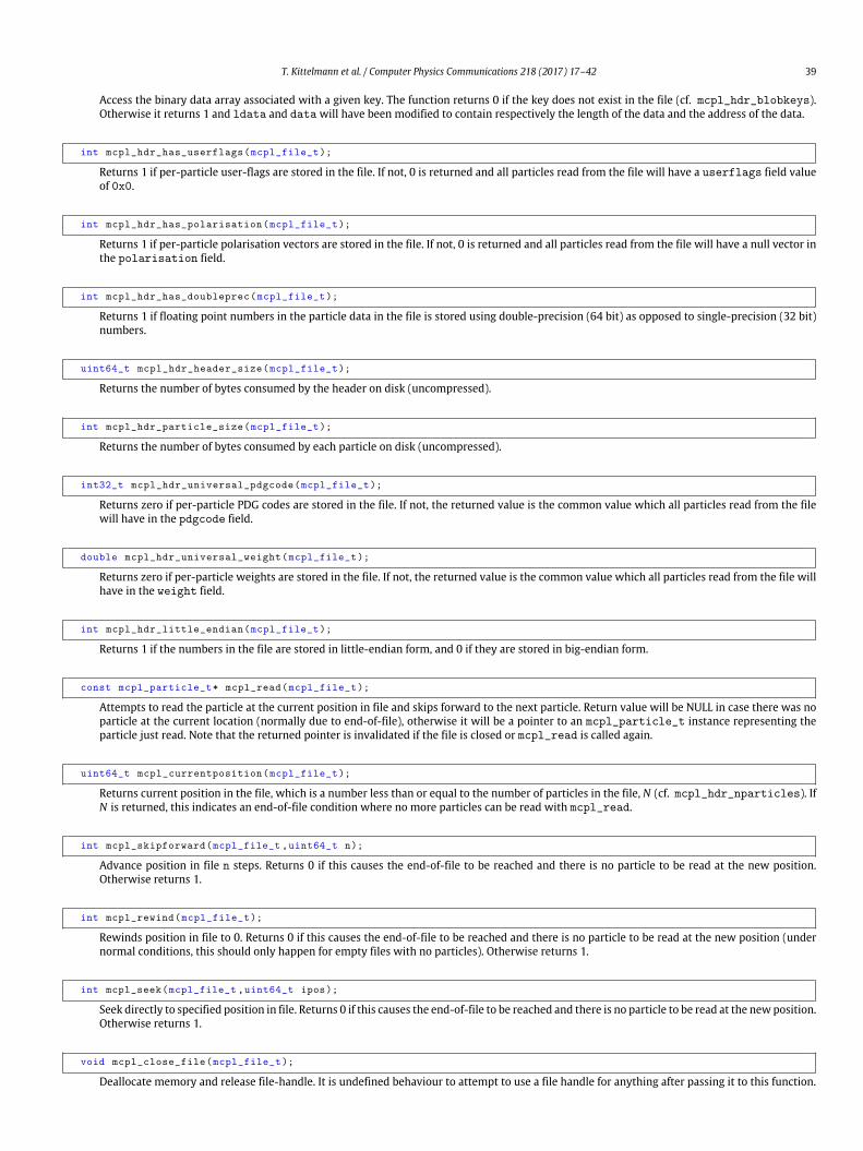
T. Kittelmann et al. / Computer Physics Communications 218 (2017) 17–42 39
Access the binary data array associated with a given key. The function returns 0 if the key does not exist in the file (cf. mcpl_hdr_blobkeys).Otherwise it returns 1 and ldata and datawill have been modified to contain respectively the length of the data and the address of the data.
int mcpl_hdr_has_userflags(mcpl_file_t);
Returns 1 if per-particle user-flags are stored in the file. If not, 0 is returned and all particles read from the file will have a userflags field valueof 0x0.
int mcpl_hdr_has_polarisation(mcpl_file_t);
Returns 1 if per-particle polarisation vectors are stored in the file. If not, 0 is returned and all particles read from the file will have a null vector inthe polarisation field.
int mcpl_hdr_has_doubleprec(mcpl_file_t);
Returns 1 if floating point numbers in the particle data in the file is stored using double-precision (64 bit) as opposed to single-precision (32 bit)numbers.
uint64_t mcpl_hdr_header_size(mcpl_file_t);
Returns the number of bytes consumed by the header on disk (uncompressed).
int mcpl_hdr_particle_size(mcpl_file_t);
Returns the number of bytes consumed by each particle on disk (uncompressed).
int32_t mcpl_hdr_universal_pdgcode(mcpl_file_t);
Returns zero if per-particle PDG codes are stored in the file. If not, the returned value is the common value which all particles read from the filewill have in the pdgcode field.
double mcpl_hdr_universal_weight(mcpl_file_t);
Returns zero if per-particle weights are stored in the file. If not, the returned value is the common value which all particles read from the file willhave in the weight field.
int mcpl_hdr_little_endian(mcpl_file_t);
Returns 1 if the numbers in the file are stored in little-endian form, and 0 if they are stored in big-endian form.
const mcpl_particle_t* mcpl_read(mcpl_file_t);
Attempts to read the particle at the current position in file and skips forward to the next particle. Return value will be NULL in case there was noparticle at the current location (normally due to end-of-file), otherwise it will be a pointer to an mcpl_particle_t instance representing theparticle just read. Note that the returned pointer is invalidated if the file is closed or mcpl_read is called again.
uint64_t mcpl_currentposition(mcpl_file_t);
Returns current position in the file, which is a number less than or equal to the number of particles in the file, N (cf. mcpl_hdr_nparticles). IfN is returned, this indicates an end-of-file condition where no more particles can be read with mcpl_read.
int mcpl_skipforward(mcpl_file_t ,uint64_t n);
Advance position in file n steps. Returns 0 if this causes the end-of-file to be reached and there is no particle to be read at the new position.Otherwise returns 1.
int mcpl_rewind(mcpl_file_t);
Rewinds position in file to 0. Returns 0 if this causes the end-of-file to be reached and there is no particle to be read at the new position (undernormal conditions, this should only happen for empty files with no particles). Otherwise returns 1.
int mcpl_seek(mcpl_file_t ,uint64_t ipos);
Seek directly to specified position in file. Returns 0 if this causes the end-of-file to be reached and there is no particle to be read at the new position.Otherwise returns 1.
void mcpl_close_file(mcpl_file_t);
Deallocate memory and release file-handle. It is undefined behaviour to attempt to use a file handle for anything after passing it to this function.
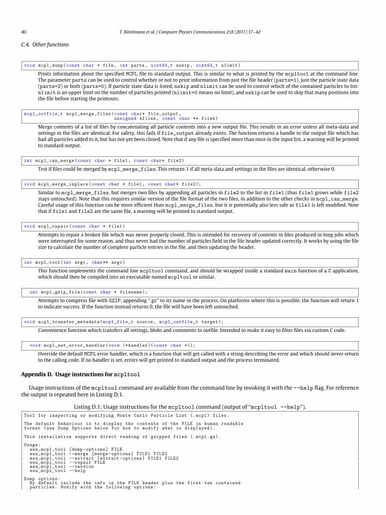
40 T. Kittelmann et al. / Computer Physics Communications 218 (2017) 17–42
C.4. Other functions
void mcpl_dump(const char * file, int parts, uint64_t nskip, uint64_t nlimit)
Prints information about the specified MCPL file to standard output. This is similar to what is printed by the mcpltool at the command line.The parameter parts can be used to control whether or not to print information from just the file header (parts=1), just the particle state data(parts=2) or both (parts=0). If particle state data is listed, nskip and nlimit can be used to control which of the contained particles to list:nlimit is an upper limit on the number of particles printed (nlimit=0means no limit), and nskip can be used to skip that many positions intothe file before starting the printouts.
mcpl_outfile_t mcpl_merge_files(const char* file_output ,unsigned nfiles, const char ** files)
Merge contents of a list of files by concatenating all particle contents into a new output file. This results in an error unless all meta-data andsettings in the files are identical. For safety, this fails if file_output already exists. The function returns a handle to the output file which hashad all particles added to it, but has not yet been closed. Note that if any file is specified more than once in the input list, a warning will be printedto standard output.
int mcpl_can_merge(const char * file1, const char* file2)
Test if files could be merged by mcpl_merge_files. This returns 1 if all meta-data and settings in the files are identical, otherwise 0.
void mcpl_merge_inplace(const char * file1, const char* file2);
Similar to mcpl_merge_files, but merges two files by appending all particles in file2 to the list in file1 (thus file1 grows while file2stays untouched). Note that this requires similar version of the file format of the two files, in addition to the other checks in mcpl_can_merge.Careful usage of this function can be more efficient than mcpl_merge_files, but it is potentially also less safe as file1 is left modified. Notethat if file1 and file2 are the same file, a warning will be printed to standard output.
void mcpl_repair(const char * file1)
Attempts to repair a broken file which was never properly closed. This is intended for recovery of contents in files produced in long jobs whichwere interrupted for some reason, and thus never had the number of particles field in the file header updated correctly. It works by using the filesize to calculate the number of complete particle entries in the file, and then updating the header.
int mcpl_tool(int argc, char** argv)
This function implements the command line mcpltool command, and should be wrapped inside a standard main function of a C application,which should then be compiled into an executable named mcpltool or similar.
int mcpl_gzip_file(const char * filename);
Attempts to compress file with GZIP, appending ‘‘.gz’’ to its name in the process. On platforms where this is possible, the function will return 1to indicate success. If the function instead returns 0, the file will have been left untouched.
void mcpl_transfer_metadata(mcpl_file_t source, mcpl_outfile_t target);
Convenience function which transfers all settings, blobs and comments to outfile. Intended to make it easy to filter files via custom C code.
void mcpl_set_error_handler(void (*handler)(const char *));
Override the default MCPL error handler, which is a function that will get called with a string describing the error and which should never returnto the calling code. If no handler is set, errors will get printed to standard output and the process terminated.
Appendix D. Usage instructions for mcpltool
Usage instructions of the mcpltool command are available from the command line by invoking it with the --help flag. For referencethe output is repeated here in Listing D.1.
Listing D.1: Usage instructions for the mcpltool command (output of ‘‘mcpltool --help’’).Tool for inspecting or modifying Monte Carlo Particle List (.mcpl) files.
The default behaviour is to display the contents of the FILE in human readableformat (see Dump Options below for how to modify what is displayed).
This installation supports direct reading of gzipped files (.mcpl.gz).
Usage:ess_mcpl_tool [dump-options] FILEess_mcpl_tool --merge [merge-options] FILE1 FILE2ess_mcpl_tool --extract [extract-options] FILE1 FILE2ess_mcpl_tool --repair FILEess_mcpl_tool --versioness_mcpl_tool --help
Dump options:By default include the info in the FILE header plus the first ten containedparticles. Modify with the following options:
T. Kittelmann et al. / Computer Physics Communications 218 (2017) 17–42 41
-j, --justhead : Dump just header info and no particle info.-n, --nohead : Dump just particle info and no header info.-lN : Dump up to N particles from the file (default 10). You
can specify -l0 to disable this limit.-sN : Skip past the first N particles in the file (default 0).-bKEY : Dump binary blob stored under KEY to standard output.
Merge options:-m, --merge FILEOUT FILE1 FILE2 ... FILEN
Creates new FILEOUT with combined particle contents fromspecified list of N existing and compatible files.
-m, --merge --inplace FILE1 FILE2 ... FILENAppends the particle contents in FILE2 ... FILEN intoFILE1. Note that this action modifies FILE1!
Extract options:-e, --extract FILE1 FILE2
Extracts particles from FILE1 into a new FILE2.-lN, -sN Select range of particles in FILE1 (as above).-pPDGCODE select particles of type given by PDGCODE.
Other options:-r, --repair FILE
Attempt to repair FILE which was not properly closed, by up-dating the file header with the correct number of particles.
-v, --version : Display version of MCPL installation.-h, --help : Display this usage information (ignores all other options).
References
[1] D.A. Kling, et al., Proceedings of the Monte Carlo 2000 Conference, Lisbon, 23–26 October 2000, Springer, 2000.[2] T. Sjöstrand, et al., in: G. Altarelli, et al. (Eds.), Z physics at LEP 1, vol. 3, CERN, Geneva, 1989, pp. 327–330. http://dx.doi.org/10.5170/CERN-1989-008-V-3.[3] M. Dobbs, J.B. Hansen, Comput. Phys. Comm. 134 (1) (2001) 41–46. http://dx.doi.org/10.1016/S0010-4655(00)00189-2.[4] J. Alwall, et al., Comput. Phys. Comm. 176 (4) (2007) 300–304. http://dx.doi.org/10.1016/j.cpc.2006.11.010.[5] T. Kittelmann, et al., Website of MCPL: Monte Carlo Particle Lists, 2016. URL: https://mctools.github.io/mcpl/.[6] K.A. Olive, et al. (Particle Data Group), Chin. Phys. C 38 (9) (2014) 090001. http://dx.doi.org/10.1088/1674-1137/38/9/090001.[7] IEEE Task P754, IEEE 754-2008, Standard for Floating-Point Arithmetic, pub-IEEE-STD, 2008, p. 58. http://dx.doi.org/10.1109/IEEESTD.2008.4610935.[8] S. Agostinelli, et al., Nucl. Instrum. Methods A 506 (2003) 250–303. http://dx.doi.org/10.1016/S0168-9002(03)01368-8.[9] J. Allison, et al., IEEE Trans. Nucl. Sci. 53 (2006) 270. http://dx.doi.org/10.1109/TNS.2006.869826.
[10] T. Kittelmann, et al., J. Phys: Conf. Ser. 513 (2014) 022017. http://dx.doi.org/10.1088/1742-6596/513/2/022017.[11] S. Peggs, et al., ESS Conceptual Design Report, ESS 2012-001, 2012. URL: http://europeanspallationsource.se/scientific-technical-documentation.[12] S. Peggs, et al., ESS Technical Design Report, ESS 2013-001, 2013. URL: http://europeanspallationsource.se/scientific-technical-documentation.[13] L.P. Deutsch, GZIP File Format Specification Version 4.3, 1952, 1996. http://dx.doi.org/10.17487/RFC1952.[14] L.P. Deutsch, DEFLATE Compressed Data Format Specification version 1.3, 1951, 1996. http://dx.doi.org/10.17487/RFC1951.[15] Jean-Loup Gailly and Mark Adler, ZLIB Compression library, 2013. URL: http://zlib.net/, v1.2.8.[16] L.P. Deutsch, J.-L. Gailly, ZLIB Compressed Data Format Specification Version 3.3, 1996. http://dx.doi.org/10.17487/RFC1950.[17] K. Lefmann, K. Nielsen, Neutron News 10 (3) (1999) 20–23. http://dx.doi.org/10.1080/10448639908233684.[18] P. Willendrup, E. Farhi, K. Lefmann, Physica B 350 (Suppl. 1–3) (2004) E735–E737. http://dx.doi.org/10.1016/j.physb.2004.03.193.[19] E. Bergbäck Knudsen, et al., J. Appl. Crystallogr. 46 (3) (2013) 679–696. http://dx.doi.org/10.1107/S0021889813007991.[20] K. Martin, B. Hoffman, Mastering CMake: A Cross-Platform Build System, Kitware Inc., 2015.[21] L.S. Waters, et al., Proceedings, Workshop, Batavia, USA, September 6–8, 2006, AIP Conf. Proc. 896 (2007) 81–90. http://dx.doi.org/10.1063/1.2720459.[22] D.B. Pelowitz, et al., MCNPX 2.7.0 Extensions, 2011.[23] B.K. Forrest Brown, J. Bull, MCNP5-1.60 Release Notes, LA-UR-10-06235, 2010.[24] J. Goorley, et al., Initial MCNP6 Release Overview - MCNP6 version 1.0, LA-UR-13-22934, 2013.[25] E. Klinkby, et al., Nucl. Instrum. Methods A 700 (2013) 106–110. http://dx.doi.org/10.1016/j.nima.2012.10.052.[26] K. Batkov, et al., mctools - Some Monte Carlo tools for MCNP(X), PHITS and FLUKA, GitHub repository, GitHub, 2015. https://github.com/kbat/mc-tools.[27] The PyNE Development Team, PyNE: The Nuclear Engineering Toolkit, 2014. URL: http://pyne.io.[28] X-5 Monte Carlo Team, MCNP - A General N-Particle Transport Code, Version 5, 2003. Volume II: User’s Guide, LA-CP-03-0245.[29] D.B. Pelowitz, MCNPX User’s Manual, Version 2.6.0, LA-CP-07-1473, 2008.[30] D.B. Pelowitz, et al., MCNP6 Users Manual, Version 1.0, LA-CP-13-00634, 2013.[31] M.P.I. Forum, MPI: A Message-Passing Interface Standard, Version 3.1, High Performance Computing Center Stuttgart (HLRS), 2015.[32] O. Kirstein, et al., Proc. Sci. (Vertex 2014) (2014) 029. arXiv:1411.6194.[33] A. Cho, Science 326 (5954) (2009) 778–779. http://dx.doi.org/10.1126/science.326_778.[34] T.M. Persons, G. Aloise, Technology Assessment: Neutron Detectors: Alternatives to Using Helium-3, GAO-11-753, 2011.[35] B. Willis, C. Carlile, Experimental Neutron Scattering, Oxford University Press, 2009.[36] A. Jackson, et al., Proceedings ICANS XXI, 2015. http://dx.doi.org/10.11484/jaea-conf-2015-002.[37] K. Kanaki, et al., J. Appl. Crystallogr. 46 (4) (2013) 1031–1037. http://dx.doi.org/10.1107/S0021889813011862.[38] K. Kanaki, et al., J. Appl. Crystallogr. 46 (4) (2013) 1528. http://dx.doi.org/10.1107/S0021889813022826.[39] SasView, SasView Model Functions, 2014. URL: http://www.sasview.org/sasview/user/models/model_functions.html, v3.0.0.[40] T. Kittelmann, M. Boin, Comput. Phys. Comm. 189 (0) (2015) 114–118. http://dx.doi.org/10.1016/j.cpc.2014.11.009.[41] L. Feigin, D. Svergun, Structure Analysis by Small-Angle X-Ray and Neutron Scattering, Springer, 1987.[42] T. Imae, et al., Neutrons in Soft Matter, Wiley, 2011.[43] T.J. Dunai, Cosmogenic Nuclides: Principles, Concepts and Applications in the Earth Surface Sciences, Cambridge University Press, 2010.[44] R. Reedy, Nucl. Instrum. Methods B 293 (2013) 470–474. http://dx.doi.org/10.1016/j.nimb.2011.08.034.[45] J. Gosse, F. Phillips, Quat. Sci. Rev. 20 (2001) 1475–1560.[46] B. Heisinger, et al., Earth Planet. Sci. Lett. 200 (2002) 345–355.[47] B. Heisinger, et al., Earth Planet. Sci. Lett. 200 (2002) 357–369.[48] J. Masarik, J. Beer, J. Geophys. Res. 104 (D10) (1999) 12099–12111.[49] J. Masarik, J. Beer, J. Geophys. Res. 114 (2009) D11103. http://dx.doi.org/10.1029/2008JD010557.[50] A. Jursa (Ed.), Handbook of Geophysics and the Space Environment, Air Force Geophys. Lab., Bedford, 1985.[51] M. Gordon, et al., IEEE Trans. Nucl. Sci. 51 (6) (2004) 3427–3434. http://dx.doi.org/10.1109/TNS.2004.839134.[52] I. Usoskin, et al., J. Geophys. Res. 110 (2005) A12108. http://dx.doi.org/10.1029/2005JA011250.

42 T. Kittelmann et al. / Computer Physics Communications 218 (2017) 17–42
[53] K. Herbst, et al., J. Geophys. Res. 115 (2010) D00I20. http://dx.doi.org/10.1029/2009JD012557.[54] Z.H. Cigolle, S. Donow, D. Evangelakos, M. Mara, M. McGuire, Q. Meyer, J. Comput. Graph. Tech. 3 (2) (2014) 1–30. URL: http://jcgt.org/published/0003/02/01/.[55] T. Engelhardt, C. Dachsbacher, Proceedings of the Vision, Modeling, and Visualization Conference 2008, VMV 2008, Konstanz, Germany, 2008, pp. 383–388.[56] F. Johansson, et al., mpmath: a Python library for arbitrary-precision floating-point arithmetic (version 0.19) mpmath, 2014. URL: http://mpmath.org/.


