November 2007

Monte Carlo Option Pricing

Victor Podlozhnyuk vpodlozhnyuk@nvidia.com Mark Harris mharris@nvidia.com

November 2007

Document Change History

Version Date Responsible Reason for Change

1.0 20/03/2007 vpodlozhnyuk Initial release

1.1 21/11/2007 mharris Rewrite with new optimizations and accuracy discussion

NVIDIA Corporation 2701 San Tomas Expressway

Santa Clara, CA 95050 www.nvidia.com

Abstract

The pricing of options has been a very important problem encountered in financial engineering since the advent of organized option trading in 1973. As more computation has been applied to finance-related problems, finding efficient implementations of option pricing models on modern architectures has become more important. This white paper describes an implementation of the Monte Carlo approach to option pricing in CUDA. For complete implementation details, please see the “MonteCarlo” example in the NVIDIA CUDA SDK.

November 2007

Introduction

The most common definition of an option is an agreement between two parties, the option seller and the option buyer, whereby the option buyer is granted a right (but not an obligation), secured by the option seller, to carry out some operation (or exercise the option) at some moment in the future. [1]

Options come in several varieties: A call option grants its holder the right to buy some underlying asset (stock, real estate, or any other good with inherent value) at a fixed predetermined price at some moment in the future. The predetermined price is referred to as the strike price, and the future date is called the expiration date. Similarly, a put option gives its holder the right to sell the underlying asset at a strike price on the expiration date.

For a call option, the profit made on the expiration date—assuming a same-day sale transaction—is the difference between the price of the asset on the expiration date and the strike price, minus the option price. For a put option, the profit made on the expiration date is the difference between the strike price and the price of the asset on the expiration date, minus the option price.

The price of the asset at expiration and the strike price therefore strongly influence how much one would be willing to pay for an option.

Other factors are:

The time to the expiration date, T: Longer periods imply wider range of possible values for the underlying asset on the expiration date, and thus more uncertainty about the value of the option.

The risk-free rate of return, R, which is the annual interest rate of Treasury Bonds or

other “risk-free” investments: any amount P of dollars is guaranteed to be worth RT

eP • dollars T years from now if placed today in one of theses investments. In other words, if an

asset is worth P dollars T years from now, it is worth RT

eP−

• today, which must be taken in account when evaluating the value of the option today.

Exercise restrictions: So far only so-called European options, which can be exercised only on the expiration date, have been discussed. But options with different types of exercise restriction also exist. For example, American-style options are more flexible as they may be exercised at any time up to and including expiration date and as such, they are generally priced at least as high as corresponding European options.

November 2007

The Monte Carlo Method in Finance

The price of the underlying asset tS follows a geometric Brownian motion with constant

driftµ and volatilityv : tttt dWSvdtSdS += µ (where tW is the Wiener random process:

),0(~0 TNWWX T −= ).

The solution of this equation is:

)(

00WWvT

Tt

t

t TeSSdWvdtS

dS −+=⇒+=

µµ .

Using the Wiener process, we can simplify this to:

)1,0(

0

),0(

0

),0(

0

2

NTvT

T

TvNT

T

TvNT

T

eSS

eSS

eSS

+

+

+

=

=

=

µ

µ

µ

(1)

The expected future value is:

TvTvTTvNT

T eSeeSeEeSSE)5.0(

0

5.0

0

),0(

0

222

)()(+

=⋅=⋅=µµµ

By definition, 2

0 5.0)( vreSSErT

T −=⇒= µ , so )1,0()5.0(

0

2NTvTvr

T eSS+−

= . This is the

possible end stock price depending on the random sample N(0, 1), which you can think of as “describing” how exactly the stock price moved.

The possible prices of derivatives at the period end are derived from the possible price of the underlying asset. For example, the price of a call option is

)0,max(),( XSTSV Tcall −= . If the market stock price at the exercise date is greater than

the strike price, a call option makes its holder a profit of XST − dollars, and zero

otherwise. Similarly, the price of a put option is )0,max(),( Tput SXTSV −= . If the

strike price at the exercise date is greater than the market stock price, a put option makes its

holder a profit of TSX − , and zero otherwise.

One method to mathematically estimate the expectation of ),( TSVcall and ),( TSVput is to

generate a large number of N(0, 1) random samples, calculate the derivative end-period prices corresponding to each of the samples, and average the generated prices:

∑=

=

N

i

imean TSVN

TSV1

),(1

),( (2)

This is the core of the Monte Carlo approach to option pricing.

Discounting the approximate future price by the discount factor Tr

e⋅−we get an

approximation of the present-day fair derivative price: Tr

meanfair eTSVSV⋅−

= ),()0,(

November 2007

In our chosen example problem, pricing European options, closed-form expressions for

)),(( TSVE call and )),(( TSVE put are known from the Black-Scholes formula [2, 3]. We

use these closed-form solutions to compute reference values for comparison against our Monte Carlo simulation results. However, the Monte Carlo approach is often applied to more complex problems, such as pricing American options, for which closed-form expressions are unknown.

Implementation

The first stage of the computation is the generation of a normally distributed pseudo-random number sequence. For this sample we use a parallel version of the Mersenne Twister random number generator [4] to generate a uniformly distributed [0, 1] sequence, and the Cartesian form of the Box-Müller transformation [5] to transform the distribution into a normal one. For more details on the efficient CUDA implementation of the Mersenne Twister and Box-Müller transformation please refer to the “MersenneTwister” sample in the CUDA SDK.

Multiple Blocks Per Option

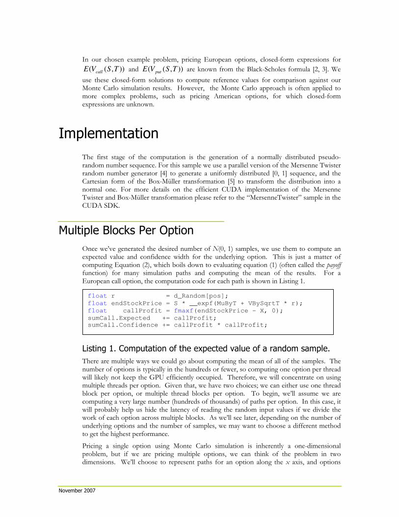
Once we’ve generated the desired number of N(0, 1) samples, we use them to compute an expected value and confidence width for the underlying option. This is just a matter of computing Equation (2), which boils down to evaluating equation (1) (often called the payoff function) for many simulation paths and computing the mean of the results. For a European call option, the computation code for each path is shown in Listing 1.

Listing 1. Computation of the expected value of a random sample.

There are multiple ways we could go about computing the mean of all of the samples. The number of options is typically in the hundreds or fewer, so computing one option per thread will likely not keep the GPU efficiently occupied. Therefore, we will concentrate on using multiple threads per option. Given that, we have two choices; we can either use one thread block per option, or multiple thread blocks per option. To begin, we’ll assume we are computing a very large number (hundreds of thousands) of paths per option. In this case, it will probably help us hide the latency of reading the random input values if we divide the work of each option across multiple blocks. As we’ll see later, depending on the number of underlying options and the number of samples, we may want to choose a different method to get the highest performance.

Pricing a single option using Monte Carlo simulation is inherently a one-dimensional problem, but if we are pricing multiple options, we can think of the problem in two dimensions. We’ll choose to represent paths for an option along the x axis, and options

float r = d_Random[pos];

float endStockPrice = S * __expf(MuByT + VBySqrtT * r);

float callProfit = fmaxf(endStockPrice - X, 0);

sumCall.Expected += callProfit; sumCall.Confidence += callProfit * callProfit;

November 2007

along the y axis. This makes it easy to determine our grid layout: we’ll launch a grid X blocks wide by Y blocks tall, where Y is the number of options we are pricing.

We also use the number of options to determine X; we want X×Y to be large enough to have plenty of thread blocks to keep the GPU busy. After some experiments on a Tesla C870 GPU, we determined a simple heuristic that gives good performance in general: if the number of options is less than 16, we use 64 blocks per option, and otherwise we use 16. Or, in code:

const int blocksPerOption = (OPT_N < 16) ? 64 : 16;

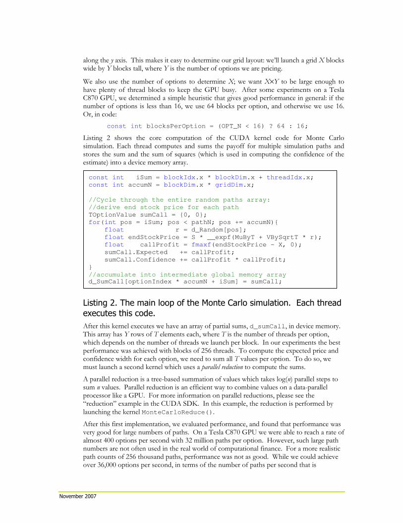
Listing 2 shows the core computation of the CUDA kernel code for Monte Carlo simulation. Each thread computes and sums the payoff for multiple simulation paths and stores the sum and the sum of squares (which is used in computing the confidence of the estimate) into a device memory array.

Listing 2. The main loop of the Monte Carlo simulation. Each thread

executes this code.

After this kernel executes we have an array of partial sums, d_sumCall, in device memory. This array has Y rows of T elements each, where T is the number of threads per option, which depends on the number of threads we launch per block. In our experiments the best performance was achieved with blocks of 256 threads. To compute the expected price and confidence width for each option, we need to sum all T values per option. To do so, we must launch a second kernel which uses a parallel reduction to compute the sums.

A parallel reduction is a tree-based summation of values which takes log(n) parallel steps to sum n values. Parallel reduction is an efficient way to combine values on a data-parallel processor like a GPU. For more information on parallel reductions, please see the “reduction” example in the CUDA SDK. In this example, the reduction is performed by launching the kernel MonteCarloReduce().

After this first implementation, we evaluated performance, and found that performance was very good for large numbers of paths. On a Tesla C870 GPU we were able to reach a rate of almost 400 options per second with 32 million paths per option. However, such large path numbers are not often used in the real world of computational finance. For a more realistic path counts of 256 thousand paths, performance was not as good. While we could achieve over 36,000 options per second, in terms of the number of paths per second that is

const int iSum = blockIdx.x * blockDim.x + threadIdx.x;

const int accumN = blockDim.x * gridDim.x;

//Cycle through the entire random paths array:

//derive end stock price for each path

TOptionValue sumCall = {0, 0};

for(int pos = iSum; pos < pathN; pos += accumN){

float r = d_Random[pos];

float endStockPrice = S * __expf(MuByT + VBySqrtT * r);

float callProfit = fmaxf(endStockPrice - X, 0);

sumCall.Expected += callProfit;

sumCall.Confidence += callProfit * callProfit;

}

//accumulate into intermediate global memory array d_SumCall[optionIndex * accumN + iSum] = sumCall;

November 2007

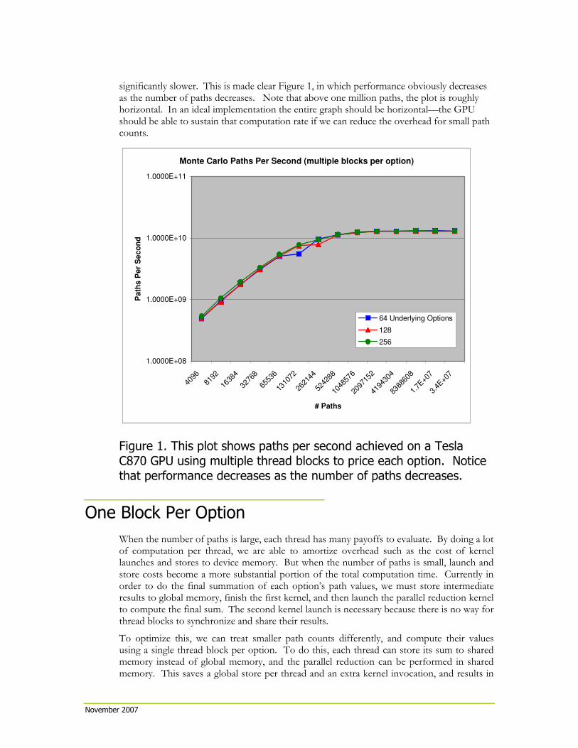
significantly slower. This is made clear Figure 1, in which performance obviously decreases as the number of paths decreases. Note that above one million paths, the plot is roughly horizontal. In an ideal implementation the entire graph should be horizontal—the GPU should be able to sustain that computation rate if we can reduce the overhead for small path counts.

Monte Carlo Paths Per Second (multiple blocks per option)

1.0000E+08

1.0000E+09

1.0000E+10

1.0000E+11

4096

8192

1638

4

3276

8

6553

6

1310

72

2621

44

5242

88

1048

576

2097

152

4194

304

8388

608

1.7E

+07

3.4E

+07

# Paths

Pa

ths

Pe

r S

ec

on

d

64 Underlying Options

128

256

Figure 1. This plot shows paths per second achieved on a Tesla

C870 GPU using multiple thread blocks to price each option. Notice

that performance decreases as the number of paths decreases.

One Block Per Option

When the number of paths is large, each thread has many payoffs to evaluate. By doing a lot of computation per thread, we are able to amortize overhead such as the cost of kernel launches and stores to device memory. But when the number of paths is small, launch and store costs become a more substantial portion of the total computation time. Currently in order to do the final summation of each option’s path values, we must store intermediate results to global memory, finish the first kernel, and then launch the parallel reduction kernel to compute the final sum. The second kernel launch is necessary because there is no way for thread blocks to synchronize and share their results.

To optimize this, we can treat smaller path counts differently, and compute their values using a single thread block per option. To do this, each thread can store its sum to shared memory instead of global memory, and the parallel reduction can be performed in shared memory. This saves a global store per thread and an extra kernel invocation, and results in

November 2007

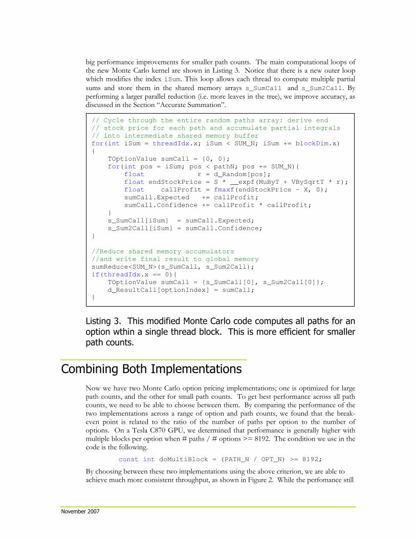
big performance improvements for smaller path counts. The main computational loops of the new Monte Carlo kernel are shown in Listing 3. Notice that there is a new outer loop which modifies the index iSum. This loop allows each thread to compute multiple partial sums and store them in the shared memory arrays s_SumCall and s_Sum2Call. By performing a larger parallel reduction (i.e. more leaves in the tree), we improve accuracy, as discussed in the Section “Accurate Summation”.

Listing 3. This modified Monte Carlo code computes all paths for an

option wthin a single thread block. This is more efficient for smaller path counts.

Combining Both Implementations

Now we have two Monte Carlo option pricing implementations; one is optimized for large path counts, and the other for small path counts. To get best performance across all path counts, we need to be able to choose between them. By comparing the performance of the two implementations across a range of option and path counts, we found that the break-even point is related to the ratio of the number of paths per option to the number of options. On a Tesla C870 GPU, we determined that performance is generally higher with multiple blocks per option when # paths / # options >= 8192. The condition we use in the code is the following.

const int doMultiBlock = (PATH_N / OPT_N) >= 8192;

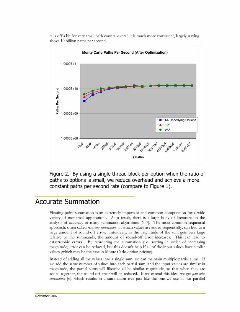
By choosing between these two implementations using the above criterion, we are able to achieve much more consistent throughput, as shown in Figure 2. While the perfomance still

// Cycle through the entire random paths array: derive end

// stock price for each path and accumulate partial integrals

// into intermediate shared memory buffer

for(int iSum = threadIdx.x; iSum < SUM_N; iSum += blockDim.x)

{

TOptionValue sumCall = {0, 0};

for(int pos = iSum; pos < pathN; pos += SUM_N){

float r = d_Random[pos];

float endStockPrice = S * __expf(MuByT + VBySqrtT * r);

float callProfit = fmaxf(endStockPrice - X, 0);

sumCall.Expected += callProfit;

sumCall.Confidence += callProfit * callProfit;

}

s_SumCall[iSum] = sumCall.Expected;

s_Sum2Call[iSum] = sumCall.Confidence;

}

//Reduce shared memory accumulators

//and write final result to global memory

sumReduce<SUM_N>(s_SumCall, s_Sum2Call);

if(threadIdx.x == 0){

TOptionValue sumCall = {s_SumCall[0], s_Sum2Call[0]};

d_ResultCall[optionIndex] = sumCall; }

November 2007

tails off a bit for very small path counts, overall it is much more consistent, largely staying above 10 billion paths per second.

Monte Carlo Paths Per Second (After Optimization)

1.0000E+08

1.0000E+09

1.0000E+10

1.0000E+11

4096

8192

1638

4

3276

8

6553

6

1310

72

2621

44

5242

88

1048

576

2097

152

4194

304

8388

608

1.7E

+07

3.4E

+07

# Paths

Path

s P

er

Seco

nd

64 Underlying Options

128

256

Figure 2. By using a single thread block per option when the ratio of

paths to options is small, we reduce overhead and achieve a more

constant paths per second rate (compare to Figure 1).

Accurate Summation

Floating point summation is an extremely important and common computation for a wide variety of numerical applications. As a result, there is a large body of literature on the analysis of accuracy of many summation algorithms [6, 7]. The most common sequential approach, often called recursive summation, in which values are added sequentially, can lead to a large amount of round-off error. Intuitively, as the magnitude of the sum gets very large relative to the summands, the amount of round-off error increases. This can lead to catastrophic errors. By reordering the summation (i.e. sorting in order of increasing magnitude) error can be reduced, but this doesn’t help if all of the input values have similar values (which may be the case in Monte Carlo option pricing).

Instead of adding all the values into a single sum, we can maintain multiple partial sums. If we add the same number of values into each partial sum, and the input values are similar in magnitude, the partial sums will likewise all be similar magnitude, so that when they are added together, the round-off error will be reduced. If we extend this idea, we get pair-wise summation [6], which results in a summation tree just like the one we use in our parallel

November 2007

reduction. Thus, not only is parallel reduction efficient on GPUs, but it can improve accuracy!

In practice, we found that by increasing the number of leaf nodes in our parallel reduction, we can significantly improve the accuracy of summation (as measured by the L1-norm of the error when comparing our GPU Monte Carlo against a double-precision CPU Monte Carlo implementation). Specifically, we reduced the L1-norm error from 7.6e-7 to 6e-8 by increasing the size of the shared memory reduction array s_SumCall from 128 to 1024 elements. The “MonteCarlo” SDK sample does not do this by default because the accuracy improvement is small compared to the error when comparing to Black-Scholes results, and because the additional accuracy comes at a performance cost of about 5%. This additional accuracy may, however, be important in real-world applications, so we provide it as an option in the code. The size of the reduction array in the code can be modified using the SUM_N parameter to sumReduce().

Monte Carlo on Multiple GPUs

Monte Carlo option pricing is “embarrassingly parallel”, because the pricing of each option is independent of all others. Therefore the computation can be distributed across multiple CUDA-capable GPUs present in the system. Monte Carlo pricing of European options with multi-GPU support is demonstrated in the “MonteCarloMultiGPU” example in the CUDA SDK. This example shares most of its CUDA code with the “MonteCarlo” example. To provide parallelism across multiple GPUs, the set of input options is divided into contiguous subsets (the number of subsets equals the number of CUDA-capable GPUs installed in the system), which are then passed to host threads driving individual GPU CUDA contexts. CUDA API state is encapsulated inside a CUDA context, so there is always a one-to-one correspondence between host threads and CUDA contexts.

Conclusion

This white paper and the “MonteCarlo” code sample in the NVIDIA SDK demonstrate that CUDA-enabled GPUs are capable of efficient and accurate Monte Carlo options pricing even for small path counts. We have shown how using performance analysis across a wide variety of problem sizes can point the way to important code optimizations. We have also demonstrated how performing more of the summation using parallel reduction and less using sequential summation in each thread can improve accuracy.

November 2007

Bibliography

1. Lai, Yongzeng and Jerome Spanier. “Applications of Monte Carlo/Quasi-Monte Carlo Methods in Finance: Option Pricing”, http://citeseer.ist.psu.edu/264429.html

2. Black, Fischer and Myron Scholes. "The Pricing of Options and Corporate Liabilities". Journal of Political Economy Vol. 81, No. 3 (1973), pp. 637-654.

3. Craig Kolb, Matt Pharr. “Option pricing on the GPU”. GPU Gems 2. (2005) Chapter 45.

4. Matsumoto, M. and T. Nishimura, "Mersenne Twister: A 623-dimensionally equidistributed uniform pseudorandom number generator", ACM Transactions on Modeling and Computer Simulation Vol. 8, No. 1 (1998), pp. 3-30.

5. Box, G. E. P. and Mervin E. Müller, “A Note on the Generation of Random Normal Deviates”, The Annals of Mathematical Statistics, Vol. 29, No. 2 (1958), pp. 610-611

6. Linz, Peter. “Accurate Floating-Point Summation”. Communications of the ACM, 13 (1970), pp. 361-362.

7. Higham, Nicholas J. “The accuracy of floating point summation”. SIAM Journal on Scientific Computing, Vol. 14, No. 4 (1993), pp. 783-799.

November 2007

Notice

ALL NVIDIA DESIGN SPECIFICATIONS, REFERENCE BOARDS, FILES, DRAWINGS, DIAGNOSTICS, LISTS, AND OTHER DOCUMENTS (TOGETHER AND SEPARATELY, “MATERIALS”) ARE BEING PROVIDED “AS IS.” NVIDIA MAKES NO WARRANTIES, EXPRESSED, IMPLIED, STATUTORY, OR OTHERWISE WITH RESPECT TO THE MATERIALS, AND EXPRESSLY DISCLAIMS ALL IMPLIED WARRANTIES OF NONINFRINGEMENT, MERCHANTABILITY, AND FITNESS FOR A PARTICULAR PURPOSE.

Information furnished is believed to be accurate and reliable. However, NVIDIA Corporation assumes no responsibility for the consequences of use of such information or for any infringement of patents or other rights of third parties that may result from its use. No license is granted by implication or otherwise under any patent or patent rights of NVIDIA Corporation. Specifications mentioned in this publication are subject to change without notice. This publication supersedes and replaces all information previously supplied. NVIDIA Corporation products are not authorized for use as critical components in life support devices or systems without express written approval of NVIDIA Corporation.

Trademarks

NVIDIA, the NVIDIA logo, GeForce, NVIDIA Quadro, and NVIDIA CUDA are trademarks or registered trademarks of NVIDIA Corporation in the United States and other countries. Other company and product names may be trademarks of the respective companies with which they are associated.

Copyright

© 2007 NVIDIA Corporation. All rights reserved.