Monte Carlo Methods

Ajay Balaji

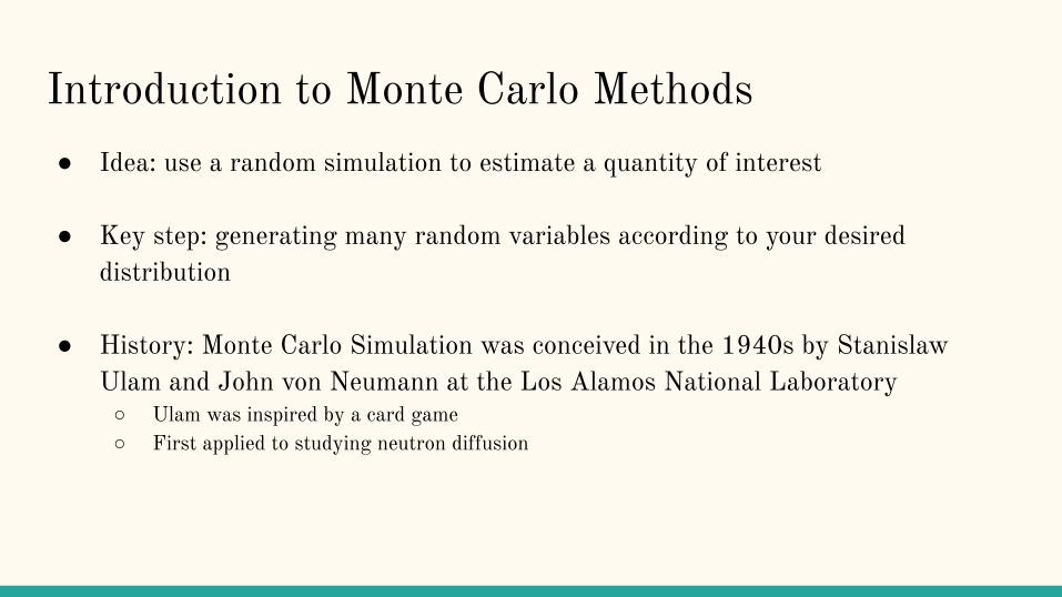
Introduction to Monte Carlo Methods● Idea: use a random simulation to estimate a quantity of interest

● Key step: generating many random variables according to your desired distribution

● History: Monte Carlo Simulation was conceived in the 1940s by Stanislaw Ulam and John von Neumann at the Los Alamos National Laboratory○ Ulam was inspired by a card game○ First applied to studying neutron diffusion

Applications● Monte Carlo methods are extremely flexible and used in a wide variety of fields● From Wikipedia:

● Whenever you want to study a distribution, MC could be useful○ Study properties, perform optimization, see how things evolve over time, etc

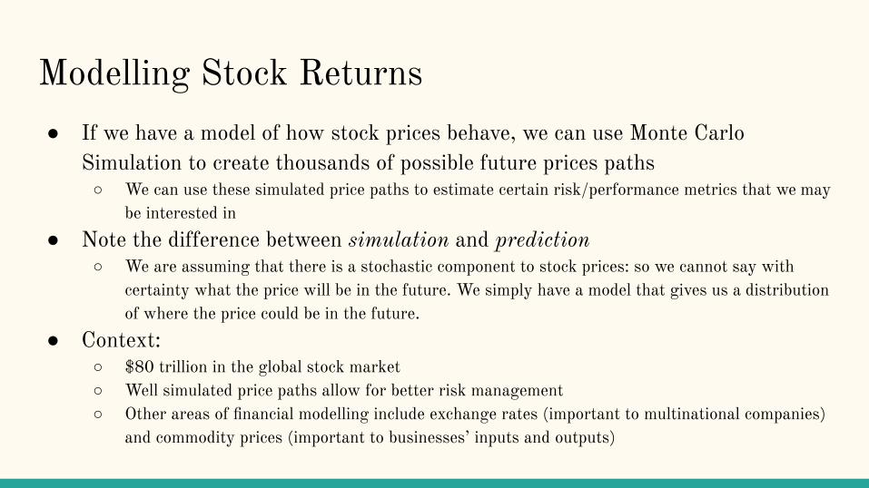
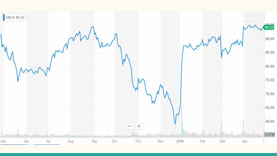
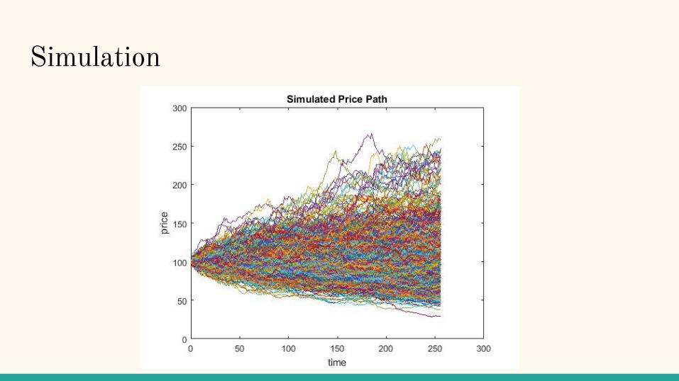
Modelling Stock Returns● If we have a model of how stock prices behave, we can use Monte Carlo

Simulation to create thousands of possible future prices paths○ We can use these simulated price paths to estimate certain risk/performance metrics that we may

be interested in● Note the difference between simulation and prediction

○ We are assuming that there is a stochastic component to stock prices: so we cannot say with certainty what the price will be in the future. We simply have a model that gives us a distribution of where the price could be in the future.

● Context:○ $80 trillion in the global stock market○ Well simulated price paths allow for better risk management○ Other areas of financial modelling include exchange rates (important to multinational companies)

and commodity prices (important to businesses’ inputs and outputs)

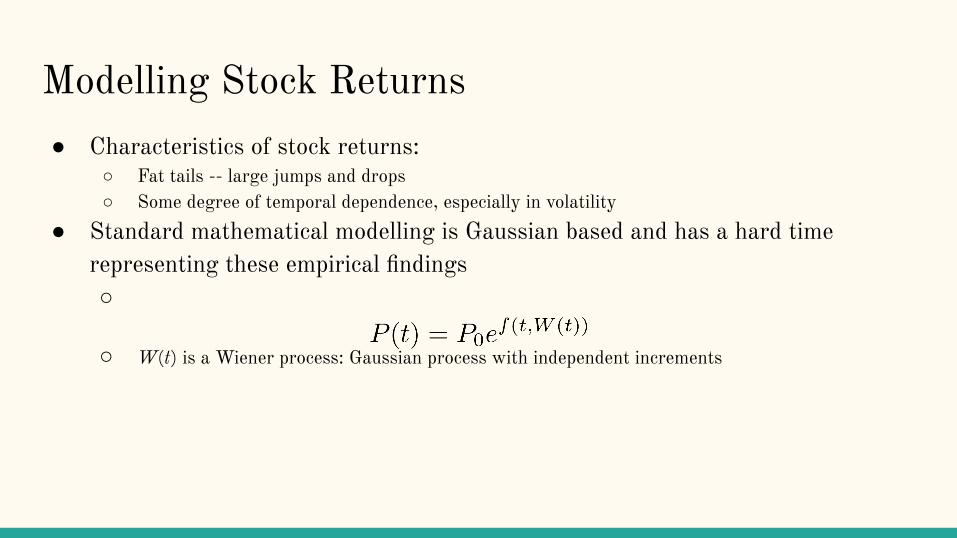
Modelling Stock Returns● Characteristics of stock returns:

○ Fat tails -- large jumps and drops○ Some degree of temporal dependence, especially in volatility

● Standard mathematical modelling is Gaussian based and has a hard time representing these empirical findings○

○ W(t) is a Wiener process: Gaussian process with independent increments

Modelling Stock Returns (cont)

Modelling Stock Returns (cont)

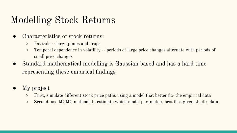
Modelling Stock Returns● Characteristics of stock returns:

○ Fat tails -- large jumps and drops○ Temporal dependence in volatility -- periods of large price changes alternate with periods of

small price changes● Standard mathematical modelling is Gaussian based and has a hard time

representing these empirical findings

● My project○ First, simulate different stock price paths using a model that better fits the empirical data○ Second, use MCMC methods to estimate which model parameters best fit a given stock’s data

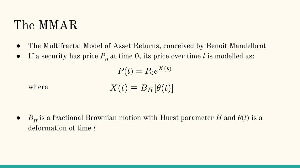
● The Multifractal Model of Asset Returns, conceived by Benoit Mandelbrot● If a security has price P0 at time 0, its price over time t is modelled as:

where

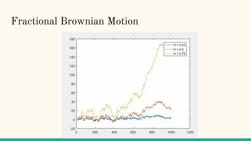
● BH is a fractional Brownian motion with Hurst parameter H and θ(t) is a deformation of time t

The MMAR

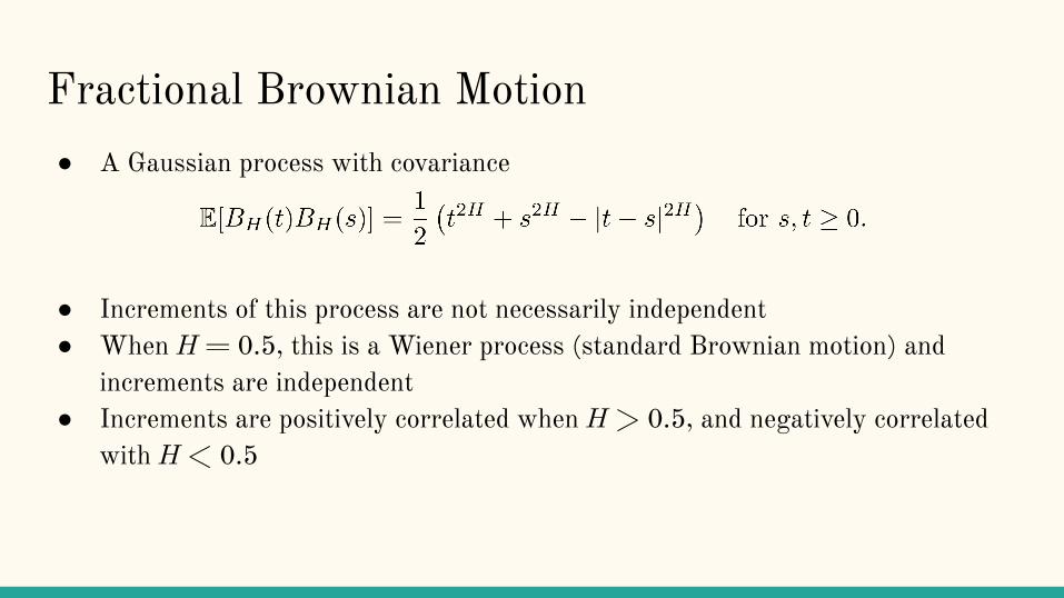
● A Gaussian process with covariance

● Increments of this process are not necessarily independent● When H = 0.5, this is a Wiener process (standard Brownian motion) and

increments are independent● Increments are positively correlated when H > 0.5, and negatively correlated

with H < 0.5

Fractional Brownian Motion

Fractional Brownian Motion

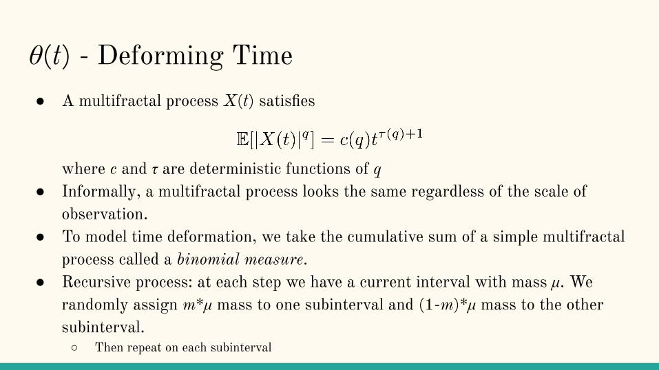
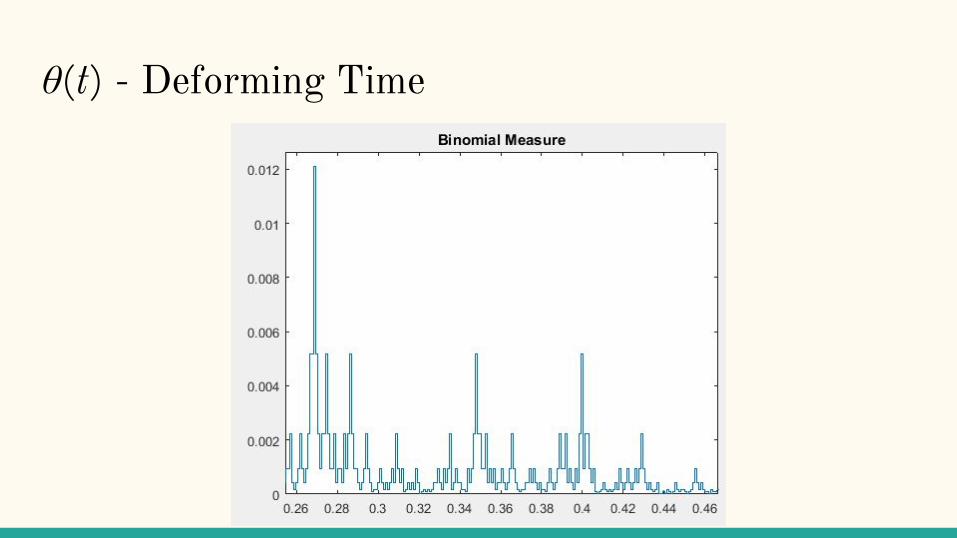
θ(t) - Deforming Time● A multifractal process X(t) satisfies

where c and τ are deterministic functions of q ● Informally, a multifractal process looks the same regardless of the scale of

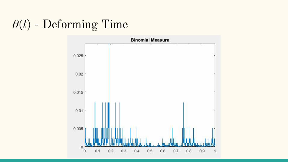
observation.● To model time deformation, we take the cumulative sum of a simple multifractal

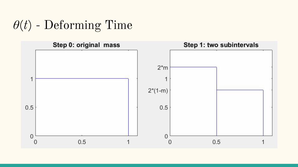
process called a binomial measure. ● Recursive process: at each step we have a current interval with mass μ. We

randomly assign m*μ mass to one subinterval and (1-m)*μ mass to the other subinterval.○ Then repeat on each subinterval

θ(t) - Deforming Time

θ(t) - Deforming Time

θ(t) - Deforming Time

θ(t) - Deforming Time

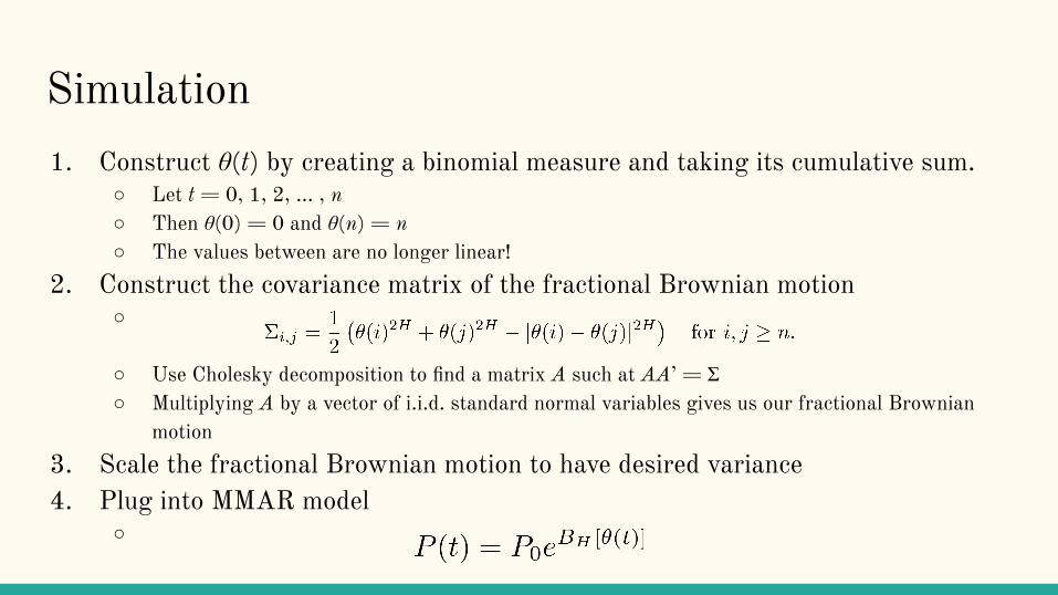
Simulation1. Construct θ(t) by creating a binomial measure and taking its cumulative sum.

○ Let t = 0, 1, 2, … , n○ Then θ(0) = 0 and θ(n) = n○ The values between are no longer linear!

2. Construct the covariance matrix of the fractional Brownian motion○

○ Use Cholesky decomposition to find a matrix A such at AA’ = Σ○ Multiplying A by a vector of i.i.d. standard normal variables gives us our fractional Brownian

motion3. Scale the fractional Brownian motion to have desired variance4. Plug into MMAR model

○

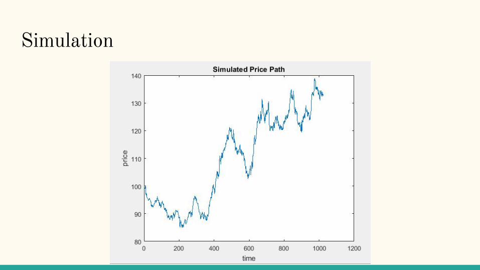
Simulation

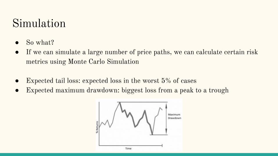
Simulation● So what?● If we can simulate a large number of price paths, we can calculate certain risk

metrics using Monte Carlo Simulation

● Expected tail loss: expected loss in the worst 5% of cases● Expected maximum drawdown: biggest loss from a peak to a trough

Simulation

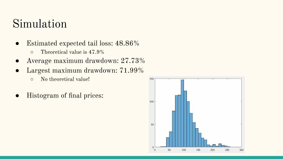
Simulation● Estimated expected tail loss: 48.86%

○ Theoretical value is 47.9%● Average maximum drawdown: 27.73%● Largest maximum drawdown: 71.99%

○ No theoretical value!

● Histogram of final prices:

Simulating a Portfolio● Consider a portfolio of n stocks, with covariance matrix Σ and weights w1, …,

wn○

● Some complications:○ Σ is a function of the stock prices and/or is random○ The weights of the portfolio are periodically updated○ Stock prices receive random occasional shocks (company earnings

announcements, political events, etc)

● What is the expected value?

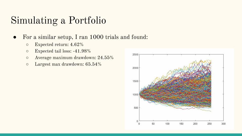
Simulating a Portfolio● For a similar setup, I ran 1000 trials and found:

○ Expected return: 4.62%○ Expected tail loss: -41.98%○ Average maximum drawdown: 24.55%○ Largest max drawdown: 65.54%

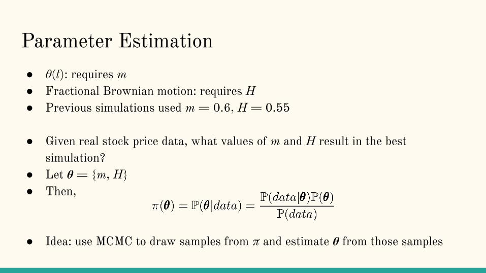
Parameter Estimation● θ(t): requires m● Fractional Brownian motion: requires H● Previous simulations used m = 0.6, H = 0.55

● Given real stock price data, what values of m and H result in the best simulation?

● Let θ = {m, H}● Then,

● Idea: use MCMC to draw samples from π and estimate θ from those samples

Markov Chain Monte Carlo● Goal: sample from a target distribution 𝛑(x)● Idea: simulate a Markov chain such that 𝛑(x) is the stationary distribution of

this chain

● A Markov chain is a sequence of random variables x(0), x(1), … that satisfy:

○ The next state depends only on the current state○ Associated transition matrix P gives transition probabilities from one state to another:

○ Certain Markov chains will converge to a stationary distribution for large values of t

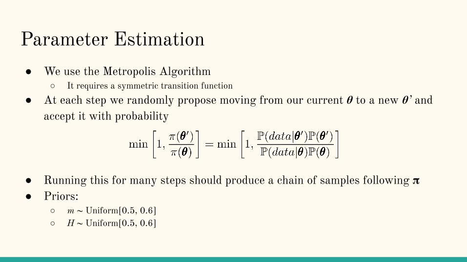
Parameter Estimation● We use the Metropolis Algorithm

○ It requires a symmetric transition function● At each step we randomly propose moving from our current θ to a new θ’ and

accept it with probability

● Running this for many steps should produce a chain of samples following 𝛑● Priors:

○ m ~ Uniform[0.5, 0.6]○ H ~ Uniform[0.5, 0.6]

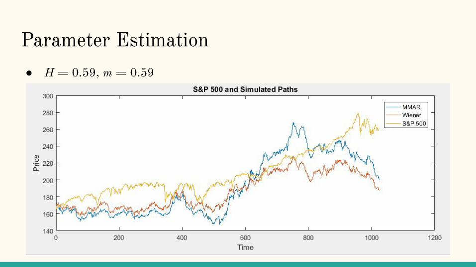
Parameter Estimation● H = 0.59, m = 0.59

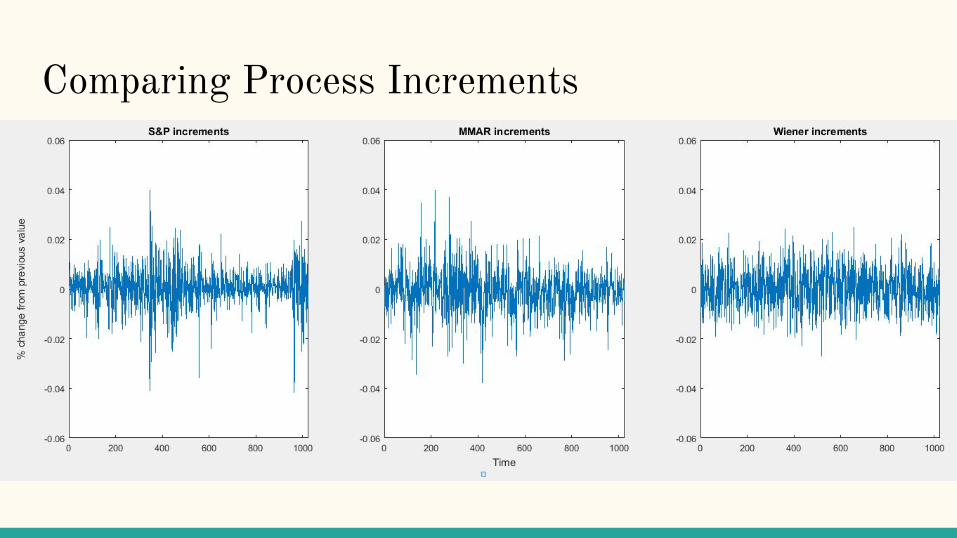
Comparing Process Increments

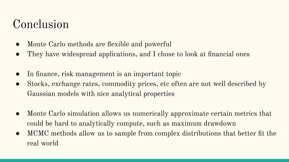
Conclusion● Monte Carlo methods are flexible and powerful● They have widespread applications, and I chose to look at financial ones

● In finance, risk management is an important topic● Stocks, exchange rates, commodity prices, etc often are not well described by

Gaussian models with nice analytical properties

● Monte Carlo simulation allows us numerically approximate certain metrics that could be hard to analytically compute, such as maximum drawdown

● MCMC methods allow us to sample from complex distributions that better fit the real world

Appendix

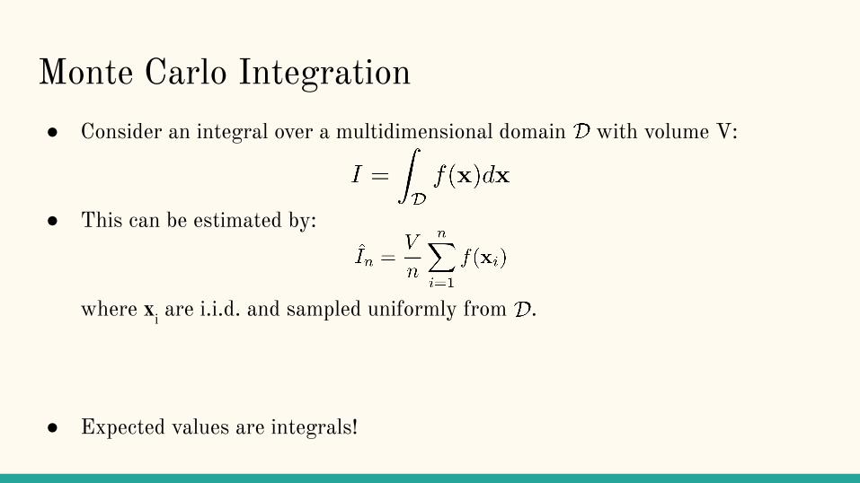
Monte Carlo Integration● Consider an integral over a multidimensional domain with volume V:

● This can be estimated by:

where xi are i.i.d. and sampled uniformly from .

● Expected values are integrals!

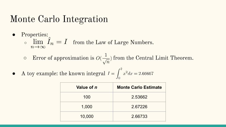
Monte Carlo Integration● Properties:

○ from the Law of Large Numbers.

○ Error of approximation is from the Central Limit Theorem.

● A toy example: the known integral

Value of n Monte Carlo Estimate

100 2.53662

1,000 2.67226

10,000 2.66733

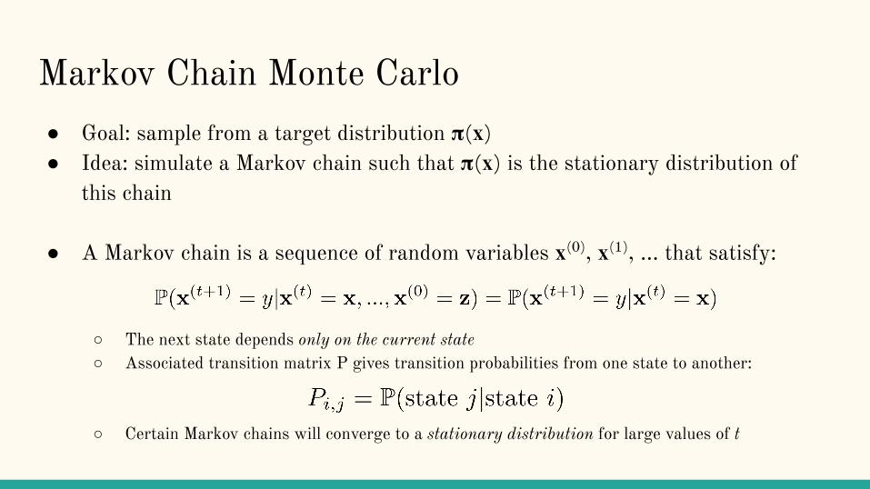
Markov Chain Monte Carlo● Goal: sample from a target distribution 𝛑(x)● Idea: simulate a Markov chain such that 𝛑(x) is the stationary distribution of

this chain

● A Markov chain is a sequence of random variables x(0), x(1), … that satisfy:

○ The next state depends only on the current state○ Associated transition matrix P gives transition probabilities from one state to another:

○ Certain Markov chains will converge to a stationary distribution for large values of t

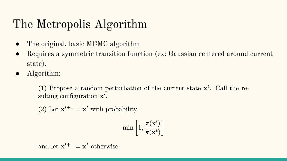
The Metropolis Algorithm● The original, basic MCMC algorithm● Requires a symmetric transition function (ex: Gaussian centered around current

state).● Algorithm:

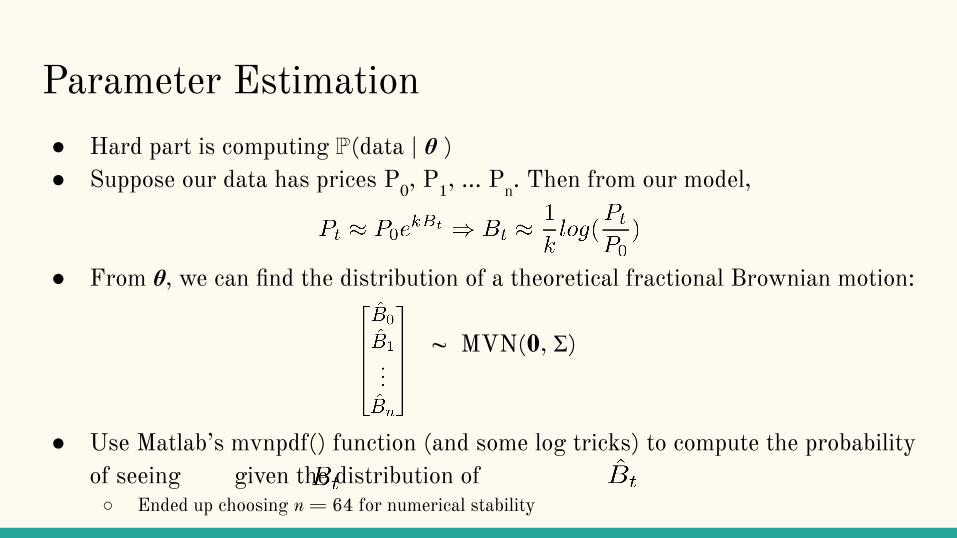
Parameter Estimation● Hard part is computing ℙ(data | θ )● Suppose our data has prices P0, P1, … Pn. Then from our model,

● From θ, we can find the distribution of a theoretical fractional Brownian motion:

~ MVN(0, Σ)

● Use Matlab’s mvnpdf() function (and some log tricks) to compute the probability of seeing given the distribution of ○ Ended up choosing n = 64 for numerical stability

References● Mandelbrot, Benoit B. and Fisher, Adlai J. and Calvet, Laurent E., A

Multifractal Model of Asset Returns (September 15, 1997). Cowles Foundation Discussion Paper No. 1164; Sauder School of Business Working Paper.

● Liu, Jun S. Monte Carlo strategies in scientific computing. Springer Science & Business Media, 2008.