Embed Size (px)
Citation preview

CS348b Lecture 10
Monte Carlo 3
Earlier lectures
■Monte Carlo I: integration using randomness
■Monte Carlo II: variance reduction
■ Basic signal processing and sampling
Today
■ Discrepancy and Quasi-Monte Carlo
■ Low-discrepancy constructions
■ Efficient implementation
Pat Hanrahan / Matt Pharr, Spring 2018

Equi-Areal Disk Sampling
CS348b Lecture 10 Pat Hanrahan / Matt Pharr, Spring 2018
✓ = 2⇡⇠1
r =p⇠2
0.2 0.4 0.6 0.8 1.0
0.2
0.4
0.6
0.8
1.0
⇠i 2 [0, 1)2

CS348b Lecture 10 Pat Hanrahan / Matt Pharr, Spring 2018
Uniform Hemisphere Sampling
p(!) =1
2⇡
(⇠1, ⇠2) ! (q
1� ⇠21 cos(2⇡⇠2),q
1� ⇠21 sin(2⇡⇠2),q
1� ⇠21)
0.2 0.4 0.6 0.8 1.0
0.2
0.4
0.6
0.8
1.0

CS348b Lecture 10 Pat Hanrahan / Matt Pharr, Spring 2018
Cosine-Weighted Hemisphere
✓ = 2⇡⇠1
r =p
⇠2
(x, y, z) = (r sin ✓, r cos ✓,p1� r2)
0.2 0.4 0.6 0.8 1.0
0.2
0.4
0.6
0.8
1.0
p(!) =cos ✓
⇡

CS348b Lecture 10
Four 2D Point Sets
Pat Hanrahan / Matt Pharr, Spring 2018
0.2 0.4 0.6 0.8 1.0
0.2
0.4
0.6
0.8
1.0
0.2 0.4 0.6 0.8 1.0
0.2
0.4
0.6
0.8
0.2 0.4 0.6 0.8 1.0
0.2
0.4
0.6
0.8
1.0
0.2 0.4 0.6 0.8 1.0
0.2
0.4
0.6
0.8
1.0

CS348b Lecture 10
Point Set Evaluation: Discrepancy
Pat Hanrahan / Matt Pharr, Spring 2018
x
y
( , )( , )
( , ) number of samples in
n x yx y xy
N
A xyn x y A
Δ = −
=
,max ( , )N x y
D x y= Δ

CS348b Lecture 10
Discrepancy
Pat Hanrahan / Matt Pharr, Spring 2018
Larscher- Pillichshammer
0.2 0.4 0.6 0.8 1.0
0.2
0.4
0.6
0.8
1.0
0.2 0.4 0.6 0.8 1.0
0.2
0.4
0.6
0.8
Stratified
0.2 0.4 0.6 0.8 1.0
0.2
0.4
0.6
0.8
Random
0.041 0.081 0.148

CS348b Lecture 10
Low-Discrepancy Definition
An (infinite) sequence of n samples in dimension d is low discrepancy if:
Pat Hanrahan / Matt Pharr, Spring 2018
Dn = O
✓(log n)d
n
◆
Dn = O
✓(log n)d�1
n
◆
A (finite) set of n samples in dimension d is low discrepancy if:
CS348b Lecture 10
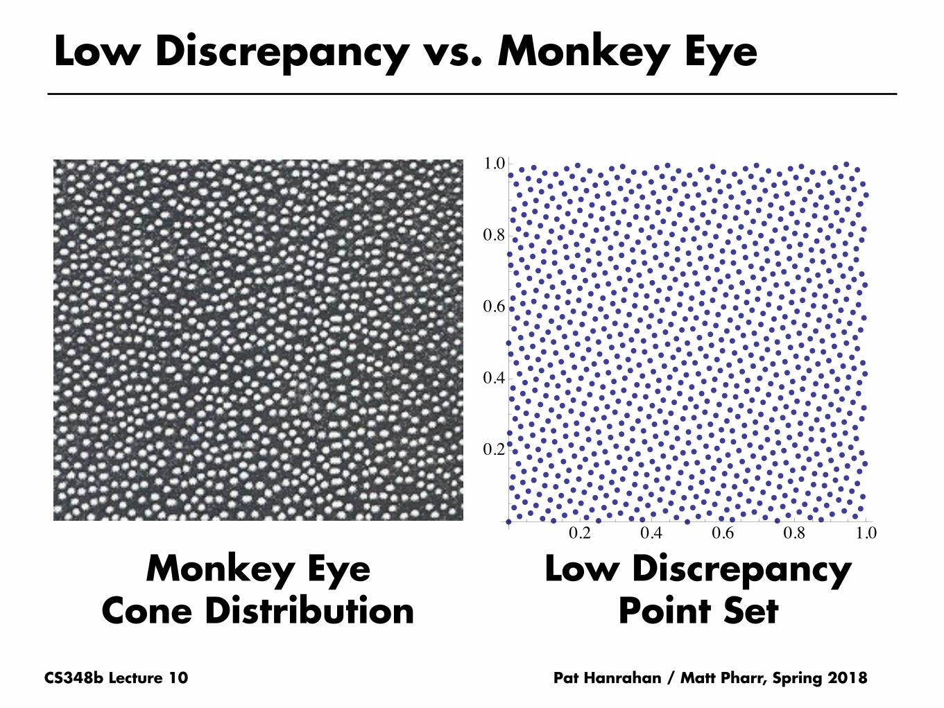
Low Discrepancy vs. Monkey Eye
Pat Hanrahan / Matt Pharr, Spring 2018
0.2 0.4 0.6 0.8 1.0
0.2
0.4
0.6
0.8
1.0
Monkey Eye Cone Distribution
Low Discrepancy Point Set
CS348b Lecture 10
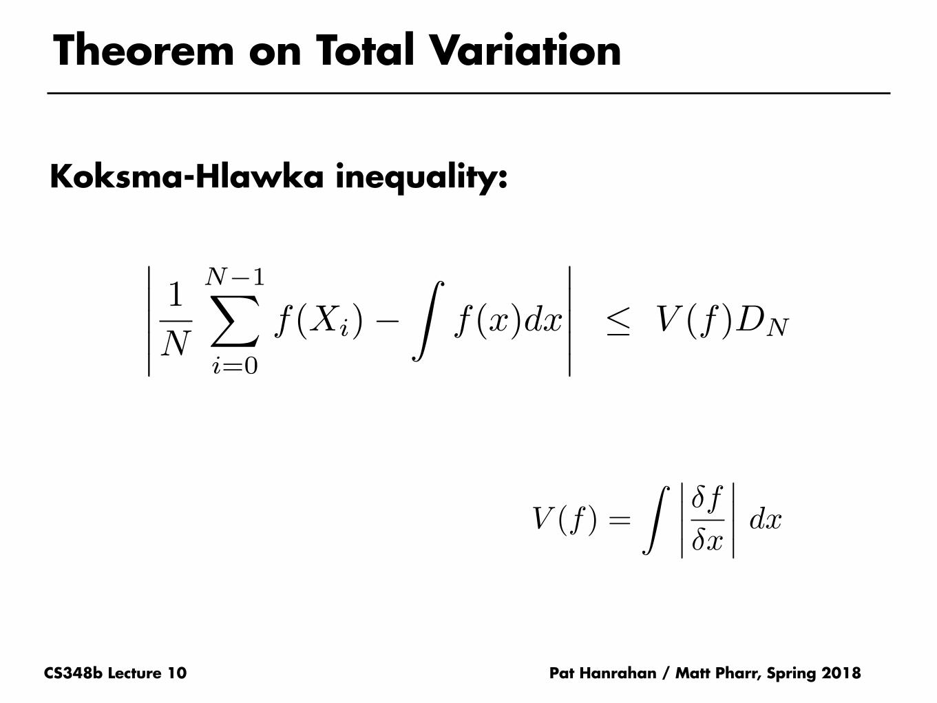
Theorem on Total Variation
Koksma-Hlawka inequality:
Pat Hanrahan / Matt Pharr, Spring 2018
�����1
N
N�1X
i=0
f(Xi)�Z
f(x)dx
����� V (f)DN
V (f) =
Z �����f
�x
���� dx

CS348b Lecture 10
Quasi-Monte Carlo Limitations
Pat Hanrahan / Matt Pharr, Spring 2018
although error bounded as: |e| V (f)DN
⇠ (log N)d
N
further, can use this inequality to show that QMC convergence is:
so, d must be small and N large to beat MC
not a tight bound!
even worse, is sometimes unbounded V (f)

CS348b Lecture 10
Measuring Point Set Quality
Some problems with low discrepancy
■ Anisotropic: rotating the points changes discrepancy
■Not shift-invariant: similarly for translation
In general, can have low discrepancy yet still have points clumped together
Pat Hanrahan / Matt Pharr, Spring 2018

Low-Discrepancy Sequences
CS348b Lecture 10
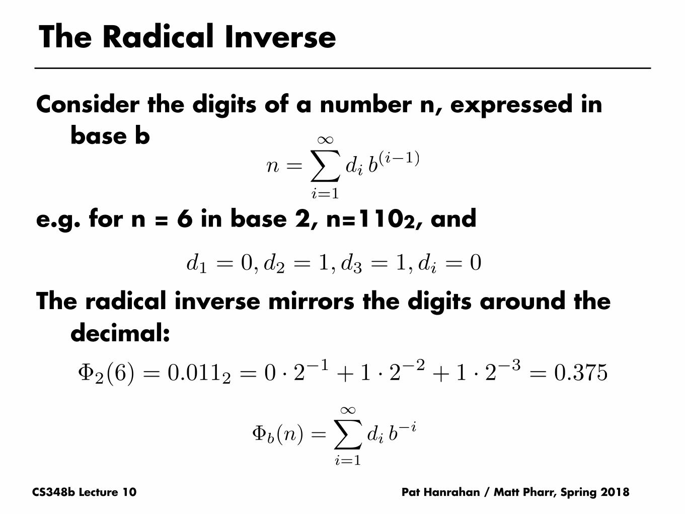
The Radical Inverse
Consider the digits of a number n, expressed in base b
e.g. for n = 6 in base 2, n=1102, and
The radical inverse mirrors the digits around the decimal:
Pat Hanrahan / Matt Pharr, Spring 2018
n =1X
i=1
di b(i�1)
d1 = 0, d2 = 1, d3 = 1, di = 0
�2(6) = 0.0112 = 0 · 2�1 + 1 · 2�2 + 1 · 2�3 = 0.375
�b(n) =1X
i=1
di b�i

CS348b Lecture 10
1D Low Discrepancy: van der Corput
Pat Hanrahan / Matt Pharr, Spring 2018
n
0 0
1 0.5
2 0.25
3 0.75
4 0.125
5 0.625
6 0.375
7 0.875
... ...
�2(n)

CS348b Lecture 10
Efficient Base 2 Radical Inverse
Assume a fixed number of bits (say 32):
We have the sum:
Pull out a factor of :
Can also express in terms of bit shifts:
Pat Hanrahan / Matt Pharr, Spring 2018
�b(n) =32X
i=1
di b�i
d1 2�1 + d2 2
�2 + · · ·+ d32 2�32
2�32 2�32(d1 231 + d2 2
30 + · · ·+ d32)
2�32((d1 << 31) + (d2 << 30) + · · ·+ d32)

CS348b Lecture 10
Efficient Base 2 Radical Inverse
We have the digits already in the bits of n
So
■ Reverse the bits
■Multiply by
Pat Hanrahan / Matt Pharr, Spring 2018
2�32((d1 << 31) + (d2 << 30) + · · ·+ d32)
n =1X
i=1
di b(i�1)
32 31 30 29 28 27 26 25 24 23 22 21 20 19 18 17 16 15 14 13 12 11 10 9 8 7 6 5 4 3 2 1
2�32

CS348b Lecture 10
uint32_t ReverseBits(uint32_t n) {
n = (n << 16) | (n >> 16);
n = ((n & 0x00ff00ff) << 8) | ((n & 0xff00ff00) >> 8);
n = ((n & 0x0f0f0f0f) << 4) | ((n & 0xf0f0f0f0) >> 4);
n = ((n & 0x33333333) << 2) | ((n & 0xcccccccc) >> 2);
n = ((n & 0x55555555) << 1) | ((n & 0xaaaaaaaa) >> 1);
return n;
}
Pat Hanrahan / Matt Pharr, Spring 2018
3231 3029 2827 2625 2423 2221 2019 1817 1615 1413 12 11 10 9 8 7 6 5 4 3 2 1
1615 1413 12 11 10 9 8 7 6 5 4 3 2 1 3231 3029 2827 2625 2423 2221 2019 1817
1615 1413 12 11 10 9 8 7 6 5 4 3 2 1 3231 3029 2827 2625 2423 2221 2019 1817
8 7 6 5 4 3 2 1 1615 1413 12 11 10 9 2423 2221 2019 1817 3231 3029 2827 2625
8 7 6 5 4 3 2 1 1615 1413 12 11 10 9 2423 2221 2019 1817 3231 3029 2827 2625
4 3 2 1 8 7 6 5 12 11 10 9 1615 1413 2019 1817 2423 2221 2827 2625 3231 3029
4 3 2 1 8 7 6 5 12 11 10 9 1615 1413 2019 1817 2423 2221 2827 2625 3231 3029
2 1 4 3 6 5 8 7 10 9 12 11 1413 1615 1817 2019 2221 2423 2625 2827 3029 3231
2 1 4 3 6 5 8 7 10 9 12 11 1413 1615 1817 2019 2221 2423 2625 2827 3029 3231
1 2 3 4 5 6 7 8 9 10 11 12 1314 1516 1718 1920 2122 2324 2526 2728 2930 3132
Reversing Bits in Parallel

CS348b Lecture 10
Efficient van Der Corput
Pat Hanrahan / Matt Pharr, Spring 2018
float RadicalInverse2(uint32_t v) {
v = ReverseBits(v);
const float Inv2To32 = 1.f / (1ull << 32);
return v * Inv2To32;
}
uint32_t ReverseBits(uint32_t n) {
n = (n << 16) | (n >> 16);
n = ((n & 0x00ff00ff) << 8) | ((n & 0xff00ff00) >> 8);
n = ((n & 0x0f0f0f0f) << 4) | ((n & 0xf0f0f0f0) >> 4);
n = ((n & 0x33333333) << 2) | ((n & 0xcccccccc) >> 2);
n = ((n & 0x55555555) << 1) | ((n & 0xaaaaaaaa) >> 1); return n;
}

CS348b Lecture 10
Radical Inverse Base 3
Pat Hanrahan / Matt Pharr, Spring 2018
n
0 0
1 0.333..
2 0.666…
3 0.111…
4 0.444…
5 0.777…
6 0.222…
7 0.555…
8 0.888…
�3(n)

Low discrepancy sequence
■ Arbitrary number of dimensions
■ Arbitrary number of points
CS348b Lecture 10
where the bases for each of the dimensions
are relatively prime
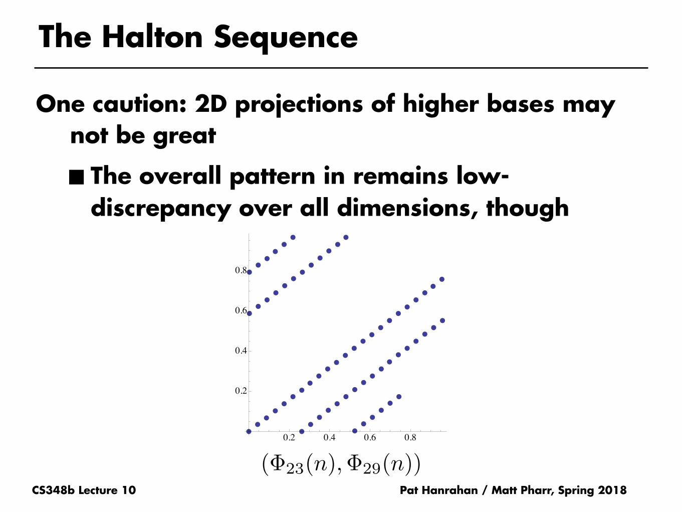
The Halton Sequence
Pat Hanrahan / Matt Pharr, Spring 2018
0.2 0.4 0.6 0.8 1.0
0.2
0.4
0.6
0.8
(�2(n),�3(n))
(�b1(n),�b2(n),�b3(n), . . .)
CS348b Lecture 10
The Halton Sequence
One caution: 2D projections of higher bases may not be great
■ The overall pattern in remains low-discrepancy over all dimensions, though
Pat Hanrahan / Matt Pharr, Spring 2018
0.2 0.4 0.6 0.8
0.2
0.4
0.6
0.8
(�23(n),�29(n))
CS348b Lecture 10
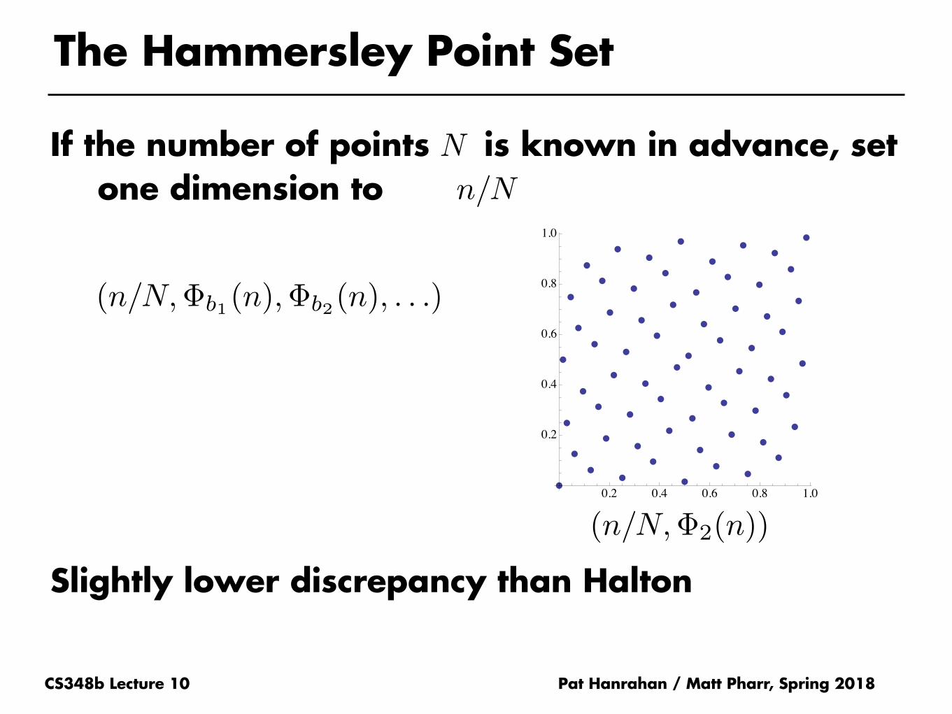
The Hammersley Point Set
If the number of points is known in advance, set one dimension to
Slightly lower discrepancy than Halton
Pat Hanrahan / Matt Pharr, Spring 2018
0.2 0.4 0.6 0.8 1.0
0.2
0.4
0.6
0.8
1.0
(n/N,�2(n))
(n/N,�b1(n),�b2(n), . . .)
n/N
N

CS348b Lecture 10
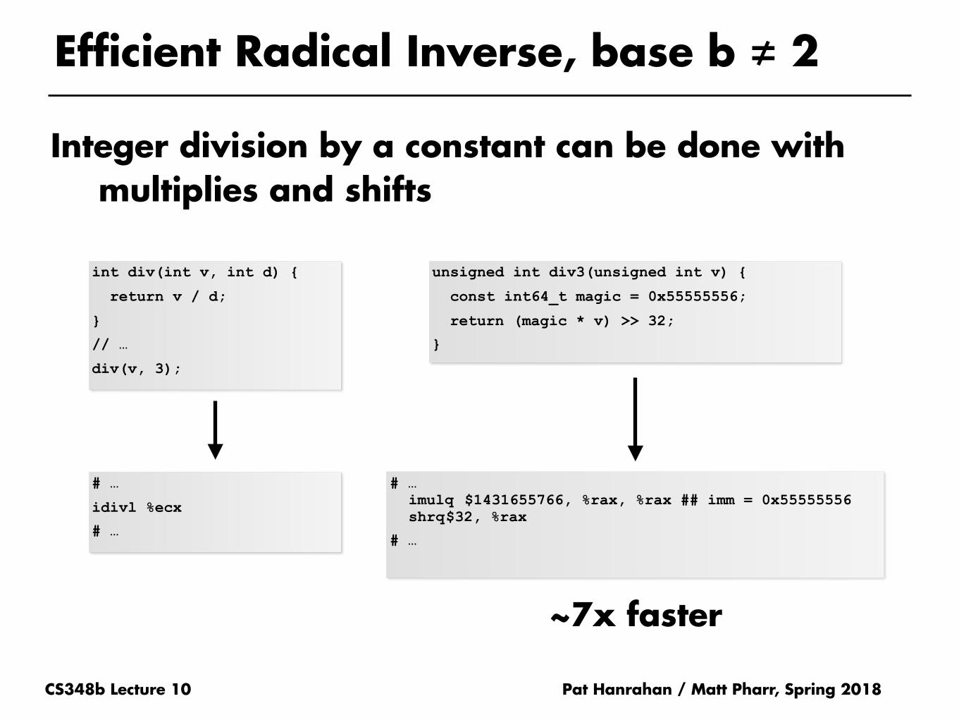
Integer division by a constant can be done with multiplies and shifts
Pat Hanrahan / Matt Pharr, Spring 2018
Efficient Radical Inverse, base b ≠ 2
unsigned int div3(unsigned int v) {
const int64_t magic = 0x55555556;
return (magic * v) >> 32;
}
q =
�232 + 2
3
n
232
⌫=
�n
3+
2n
3⇥ 232
⌫
=jn3
kif n < 232
CS348b Lecture 10
Integer division by a constant can be done with multiplies and shifts
Pat Hanrahan / Matt Pharr, Spring 2018
int div(int v, int d) {
return v / d;
}
// …
div(v, 3);
# …
idivl %ecx
# …
# … imulq $1431655766, %rax, %rax ## imm = 0x55555556 shrq $32, %rax
# …
~7x faster
Efficient Radical Inverse, base b ≠ 2
unsigned int div3(unsigned int v) {
const int64_t magic = 0x55555556;
return (magic * v) >> 32;
}

CS348b Lecture 10
Generator Matrices
Given a base b and a matrix C, define:
■where di are the base-b digits of n
■ and arithmetic is done over the ring
■ For our purposes, just do everything “mod b”
This generates a set of bm points
Appropriately-chosen C matrices generate various low-discrepancy point sets
Pat Hanrahan / Matt Pharr, Spring 2018
Zb
c(n) = (b�1, b�2, . . . , b�m)C
0
BBB@
d1d2...
dm
1
CCCA

CS348b Lecture 10
Generator Matrices
We’ll focus only on b=2, which allows particularly efficient implementation
Pat Hanrahan / Matt Pharr, Spring 2018
c(n) = (2�1, 2�2, . . . , 2�m)C
0
BBB@
d1d2...
dm
1
CCCA

CS348b Lecture 10
Sobol’ Point Sets
Sobol’ first showed how to find generator matrices for LD point sets in base 2
■ Can scale low-discrepancy samples in 1000s of dimensions
Pat Hanrahan / Matt Pharr, Spring 2018
1 10 20 32
1
10
20
32
1 10 20 32
1
10
20
32
1 10 20 32
1
10
20
32
1 10 20 32
1
10
20
32
1 10 20 32
1
10
20
32
1 10 20 32
1
10
20
32
1 10 20 32
1
10
20
32
1 10 20 32
1
10
20
32
1 10 20 32
1
10
20
32
1 10 20 32
1
10
20
32
C0 C1 C2 C3 C4
...

CS348b Lecture 10
32 2D Sobol’ Points
Pat Hanrahan / Matt Pharr, Spring 2018
0.2 0.4 0.6 0.8
0.2
0.4
0.6
0.8
CS348b Lecture 10
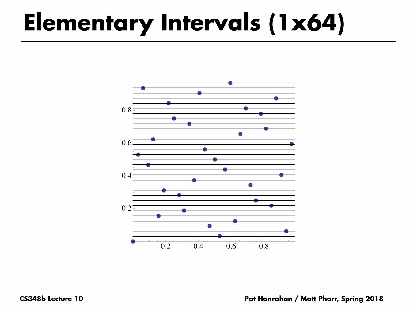
Elementary Intervals (1x64)
Pat Hanrahan / Matt Pharr, Spring 2018
0.2 0.4 0.6 0.8
0.2
0.4
0.6
0.8

CS348b Lecture 10
Elementary Intervals (2x32)
Pat Hanrahan / Matt Pharr, Spring 2018
0.2 0.4 0.6 0.8
0.2
0.4
0.6
0.8

CS348b Lecture 10
Elementary Intervals (4x8)
Pat Hanrahan / Matt Pharr, Spring 2018
0.2 0.4 0.6 0.8
0.2
0.4
0.6
0.8

CS348b Lecture 10
Elementary Intervals (8x4)
Pat Hanrahan / Matt Pharr, Spring 2018
0.2 0.4 0.6 0.8
0.2
0.4
0.6
0.8

CS348b Lecture 10
Elementary Intervals (16x2)
Pat Hanrahan / Matt Pharr, Spring 2018
0.2 0.4 0.6 0.8
0.2
0.4
0.6
0.8

CS348b Lecture 10
Elementary Intervals (32x1)
Pat Hanrahan / Matt Pharr, Spring 2018
0.2 0.4 0.6 0.8
0.2
0.4
0.6
0.8

Uniform Random Samples, n=16 MSE 0.00227214
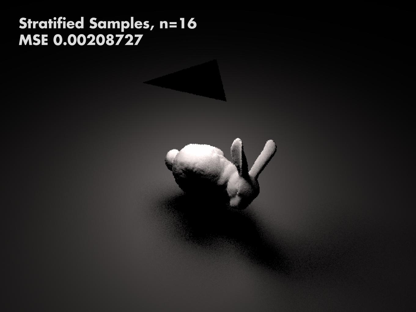
Stratified Samples, n=16 MSE 0.00208727

Low Discrepancy Samples, n=16 MSE 0.00201494

Uniform Random Samples, n=16 MSE 0.000421827

Stratified Samples, n=16 MSE 0.000253177

Low Discrepancy Samples, n=16 MSE 0.000164011
CS348b Lecture 10
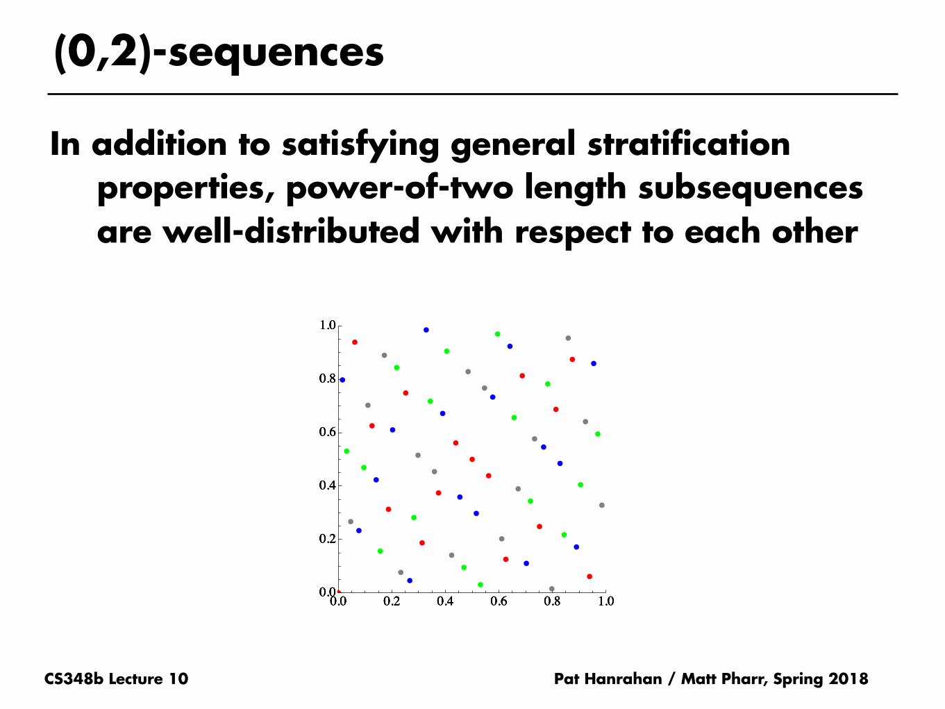
(0,2)-sequences
In addition to satisfying general stratification properties, power-of-two length subsequences are well-distributed with respect to each other
Pat Hanrahan / Matt Pharr, Spring 2018
0.0 0.2 0.4 0.6 0.8 1.00.0
0.2
0.4
0.6
0.8
1.0
0.0 0.2 0.4 0.6 0.8 1.00.0
0.2
0.4
0.6
0.8
1.0
0.0 0.2 0.4 0.6 0.8 1.00.0
0.2
0.4
0.6
0.8
1.0
0.0 0.2 0.4 0.6 0.8 1.00.0
0.2
0.4
0.6
0.8
1.0

CS348b Lecture 10
Pixel * Light Sampling
Pat Hanrahan / Matt Pharr, Spring 2018
0.0 0.2 0.4 0.6 0.8 1.00.0
0.2
0.4
0.6
0.8
1.0
0.0 0.2 0.4 0.6 0.8 1.00.0
0.2
0.4
0.6
0.8
1.0
0.0 0.2 0.4 0.6 0.8 1.00.0
0.2
0.4
0.6
0.8
1.0
0.0 0.2 0.4 0.6 0.8 1.00.0
0.2
0.4
0.6
0.8
1.0

CS348b Lecture 10
Maximized Minimum Distance
Grünschloß and Keller: exhaustive search over generator matrices
Pat Hanrahan / Matt Pharr, Spring 2018
0.2 0.4 0.6 0.8 1.0
0.2
0.4
0.6
0.8
1.0
Sobol’Min Dist 0.044
0.2 0.4 0.6 0.8 1.0
0.2
0.4
0.6
0.8
1.0
Min Dist 0.112
Still stratified over elementary intervals
C6 =
0
BBBBBB@
1 0 0 0 0 01 1 0 0 0 01 1 1 0 0 00 0 0 1 1 00 0 1 0 1 00 0 0 0 0 1
1
CCCCCCA

CS348b Lecture 10
Sobol’ Points Power Spectrum
Pat Hanrahan / Matt Pharr, Spring 2018
Sobol’

CS348b Lecture 10
Low Discrepancy + Blue Noise
Pat Hanrahan / Matt Pharr, Spring 2018
Ahmed et al. 2016
CS348b Lecture 10
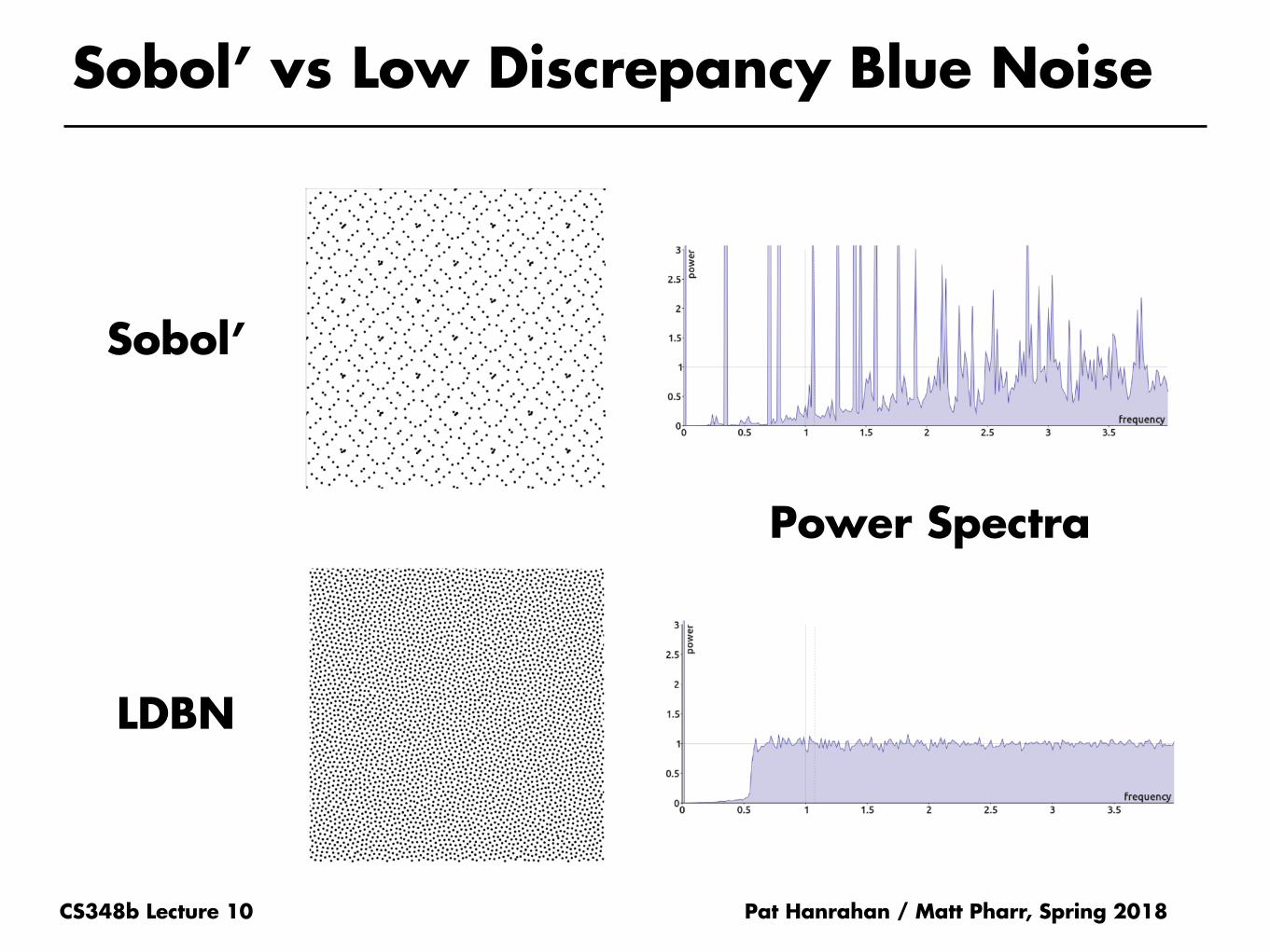
Sobol’ vs Low Discrepancy Blue Noise
Pat Hanrahan / Matt Pharr, Spring 2018
Sobol’
LDBN
Power Spectra

(Live demo)
CS348b Lecture 10
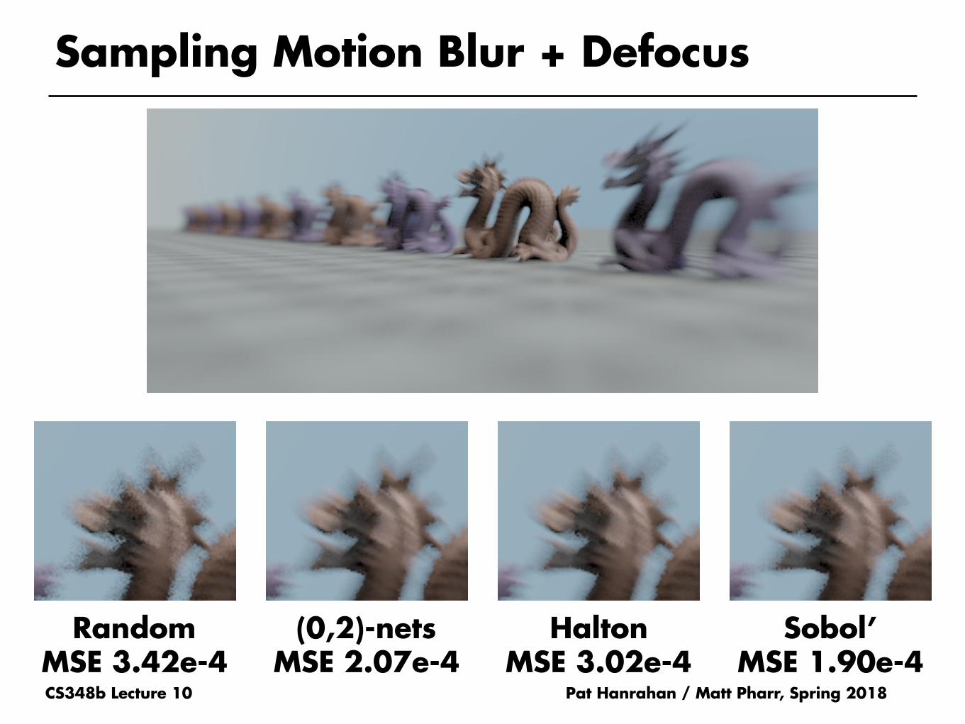
Sampling Motion Blur + Defocus
Pat Hanrahan / Matt Pharr, Spring 2018
Sobol’ MSE 1.90e-4
Halton MSE 3.02e-4
(0,2)-nets MSE 2.07e-4
Random MSE 3.42e-4
CS348b Lecture 10
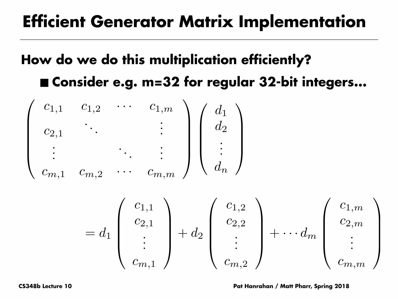
Efficient Generator Matrix Implementation
How do we do this multiplication efficiently?
■ Consider e.g. m=32 for regular 32-bit integers...
Pat Hanrahan / Matt Pharr, Spring 2018
0
BBBB@
c1,1 c1,2 · · · c1,m
c2,1. . .
......
. . ....
cm,1 cm,2 · · · cm,m
1
CCCCA
0
BBB@
d1d2...dn
1
CCCA
= d1
0
BBB@
c1,1c2,1...
cm,1
1
CCCA+ d2
0
BBB@
c1,2c2,2...
cm,2
1
CCCA+ · · · dm
0
BBB@
c1,mc2,m...
cm,m
1
CCCA

CS348b Lecture 10
Recall that we’re doing all of this arithmetic mod 2
■ All values are either 0 or 1...
Pat Hanrahan / Matt Pharr, Spring 2018
d1
0
BBB@
c1,1c2,1...
cm,1
1
CCCA+ d2
0
BBB@
c1,2c2,2...
cm,2
1
CCCA+ · · · dm
0
BBB@
c1,mc2,m...
cm,m
1
CCCA
+ 0 1
0 0 1
1 1 0
* 0 1
0 0 0
1 0 1
▪ What logical ops are + and *, mod 2, equivalent to?
Efficient Generator Matrix Implementation
CS348b Lecture 10 Pat Hanrahan / Matt Pharr, Spring 2018
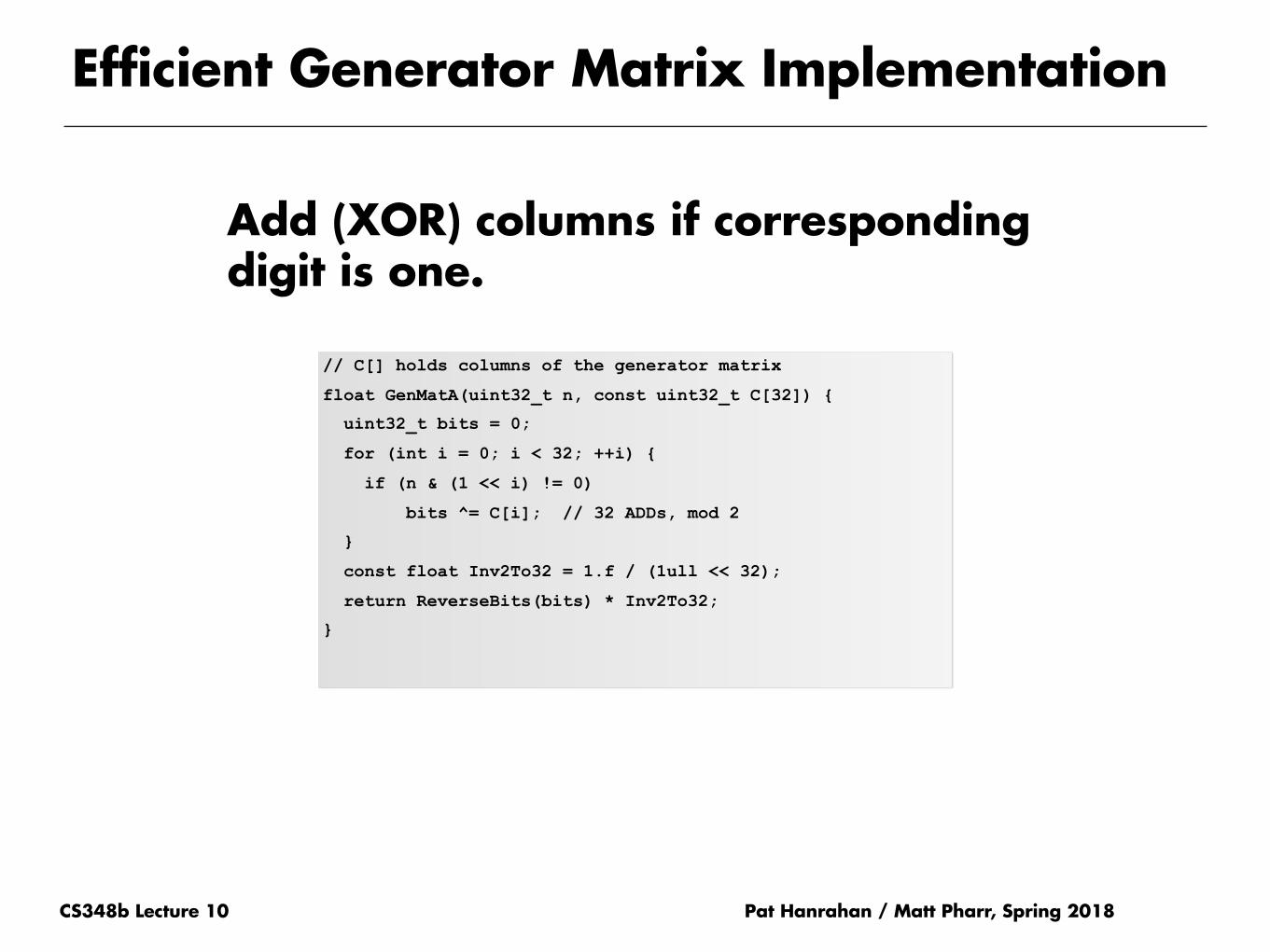
// C[] holds columns of the generator matrix
float GenMatA(uint32_t n, const uint32_t C[32]) {
uint32_t bits = 0;
for (int i = 0; i < 32; ++i) {
if (n & (1 << i) != 0)
bits ^= C[i]; // 32 ADDs, mod 2
}
const float Inv2To32 = 1.f / (1ull << 32);
return ReverseBits(bits) * Inv2To32;
}
Add (XOR) columns if corresponding digit is one.
Efficient Generator Matrix Implementation

CS348b Lecture 10 Pat Hanrahan / Matt Pharr, Spring 2018
float GenMatB(uint32_t n, const uint32_t C[32]) {
uint32_t bits = 0, i = 0;
while (n != 0) {
if (n & 1)
bits ^= C[i];
n >>= 1;
++i;
}
const float Inv2To32 = 1.f / (1ull << 32);
return ReverseBits(bits) * Inv2To32;
}
Better: stop when n=0
Efficient Generator Matrix Implementation

CS348b Lecture 10 Pat Hanrahan / Matt Pharr, Spring 2018
float GenMatB(uint32_t n, const uint32_t C[32]) {
uint32_t bits = 0, i = 31;
while (n != 0) {
if (n & 1)
bits ^= C[i];
n >>= 1;
--i;
}
const float Inv2To32 = 1.f / (1ull << 32);
return bits * Inv2To32;
}
Avoid the bit reverse by reversing the columns of the matrix
Efficient Generator Matrix Implementation

CS348b Lecture 10
Even Faster Evaluation with Grey Codes
Grey codes: permutation of integers within blocks of size 2n such that adjacent values only differ in a single bit
Very simple to compute:
Pat Hanrahan / Matt Pharr, Spring 2018
int GreyCode(int v) {
return v ^ (v >> 1);
}
n binary Grey code
0 0 0
1 1 1
2 10 11
3 11 10
4 100 110
5 101 111
6 110 101
7 111 100
8 1000 1100
... ... ...
CS348b Lecture 10
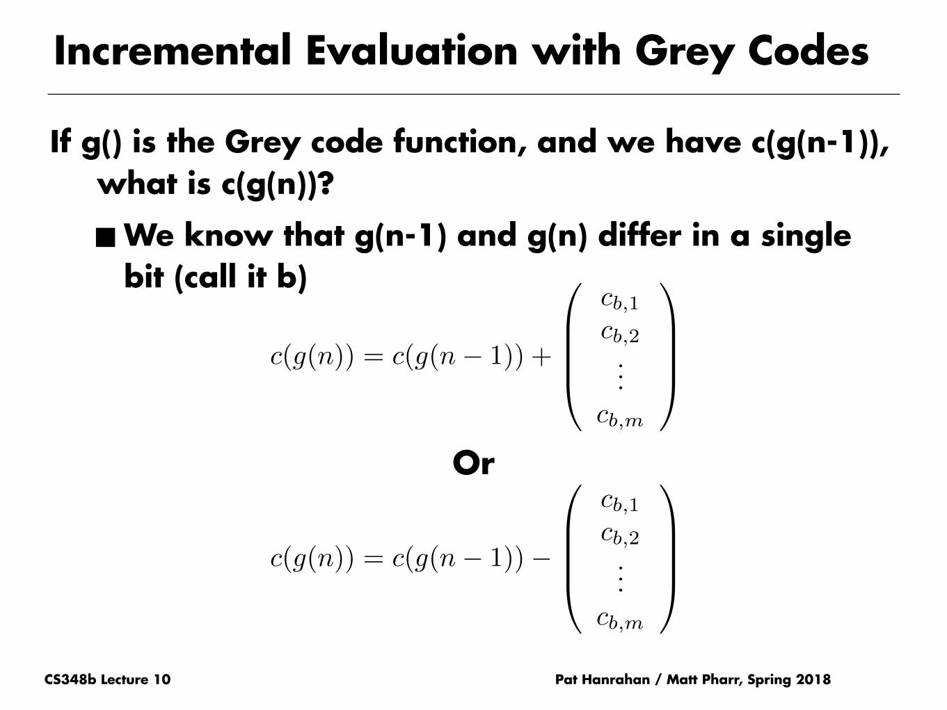
Incremental Evaluation with Grey Codes
If g() is the Grey code function, and we have c(g(n-1)), what is c(g(n))?
■We know that g(n-1) and g(n) differ in a single bit (call it b)
Pat Hanrahan / Matt Pharr, Spring 2018
c(g(n)) = c(g(n� 1)) +
0
BBB@
cb,1cb,2...
cb,m
1
CCCA
c(g(n)) = c(g(n� 1))�
0
BBB@
cb,1cb,2...
cb,m
1
CCCA
Or
CS348b Lecture 10
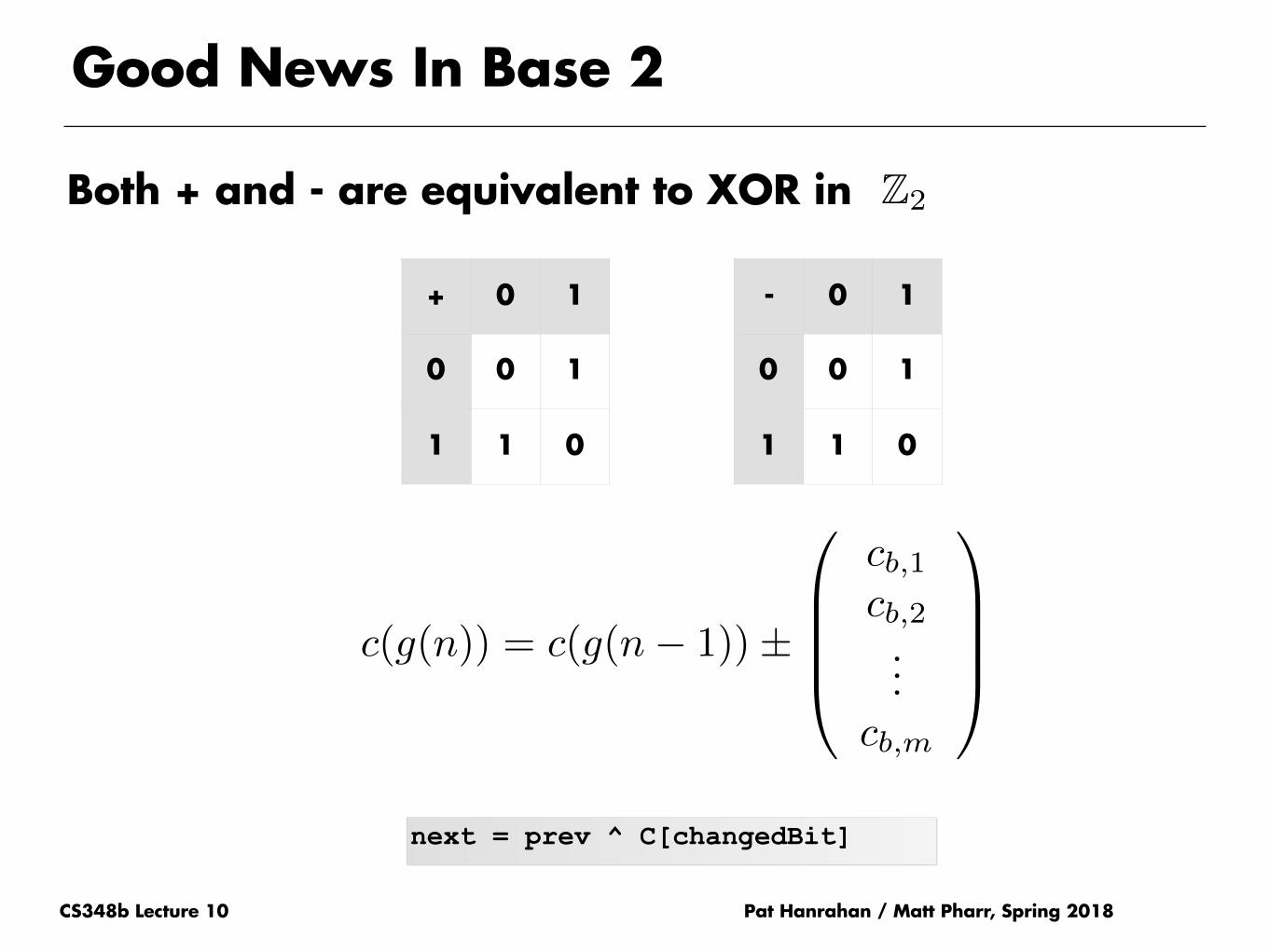
Good News In Base 2
Both + and - are equivalent to XOR in
Pat Hanrahan / Matt Pharr, Spring 2018
+ 0 1
0 0 1
1 1 0
- 0 1
0 0 1
1 1 0
Z2
next = prev ^ C[changedBit]
c(g(n)) = c(g(n� 1))±
0
BBB@
cb,1cb,2...
cb,m
1
CCCA

CS348b Lecture 10
Even Faster Evaluation with Grey Codes
Pat Hanrahan / Matt Pharr, Spring 2018
Which Bit Changed?
n/a
0
1
0
2
0
1
0
3
...
# of trailing 0s in the binary
representation of n
n binary Grey code
0 0 0
1 1 1
2 10 11
3 11 10
4 100 110
5 101 111
6 110 101
7 111 100
8 1000 1100
... ... ...
CS348b Lecture 10
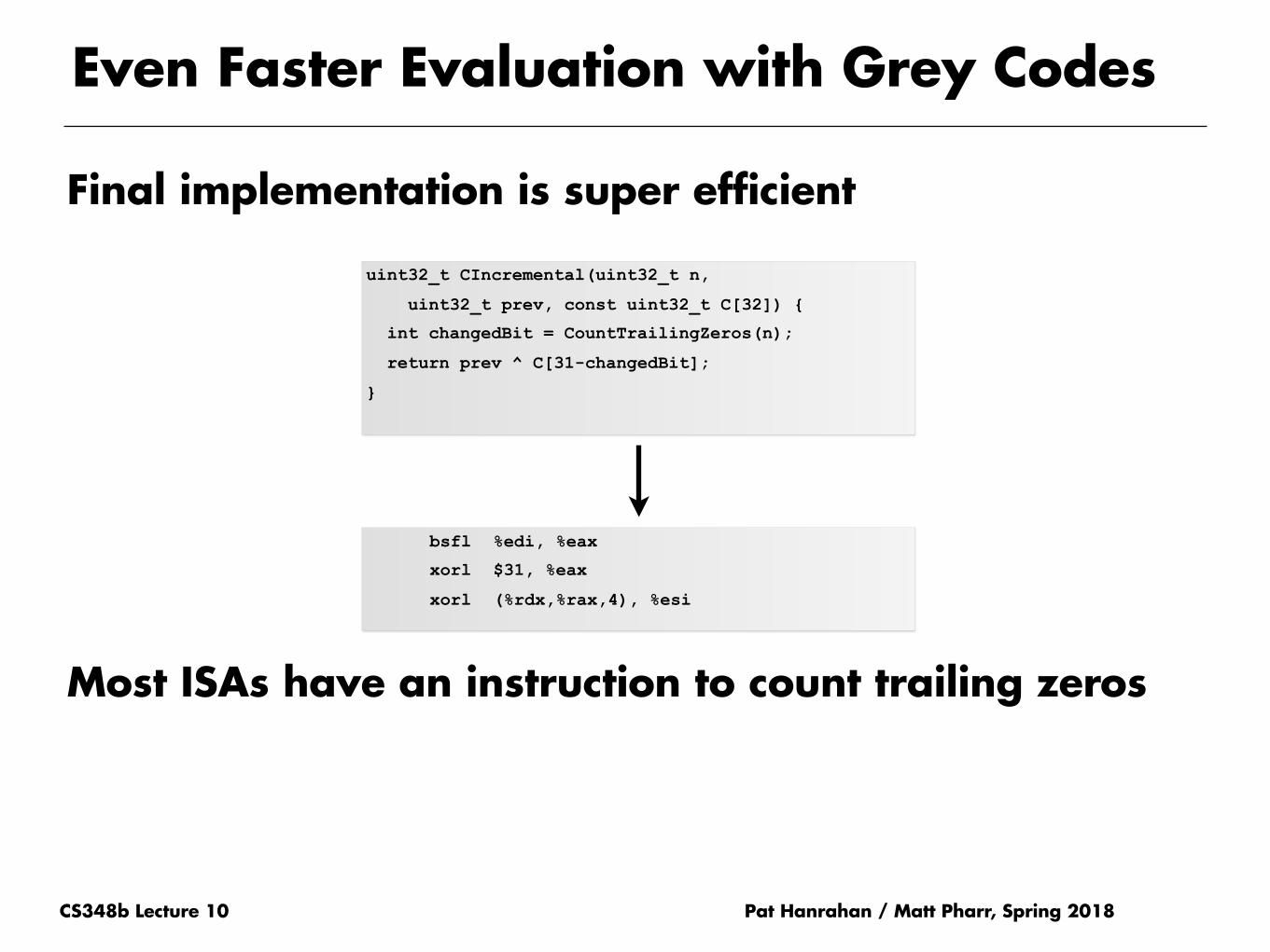
Even Faster Evaluation with Grey Codes
Final implementation is super efficient
Most ISAs have an instruction to count trailing zeros
Pat Hanrahan / Matt Pharr, Spring 2018
uint32_t CIncremental(uint32_t n,
uint32_t prev, const uint32_t C[32]) {
int changedBit = CountTrailingZeros(n);
return prev ^ C[31-changedBit];
}
bsfl %edi, %eax
xorl $31, %eax
xorl (%rdx,%rax,4), %esi


