Money, Finance and Growth

Ping Wang©

Department of EconomicsWashington University in St. Louis

April 2017

A. Introduction

I. Empirical Regularities

1. Money and growth (Friedman-Schwartz; Walsh, ch. 1):

a. positive correlation in levelsb. largely negative correlation in growth ratesc. presence of a liquidity effect

1

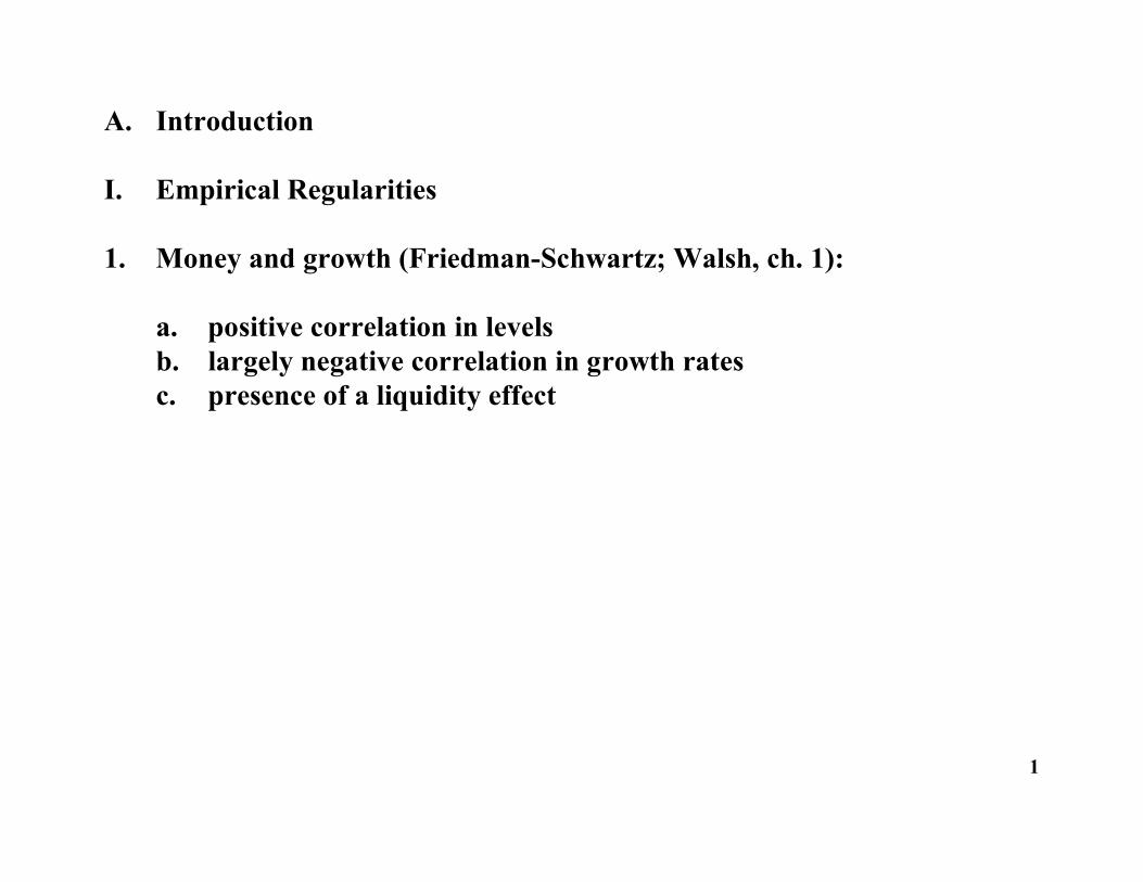
Summer-Heston data (1960-85, excluding poor quality data, 60 countries):

Note: (i) High inflation countries: 28 = Indonesia, 46 = Iceland, 57 = Turkey,17 = Mexico, 21 = Columbia;

(ii) High growth countries: 26 = Hong Kong, 34 = Singapore, 3 =Morocco, 30 = South Korea, 29 = Japan.

2

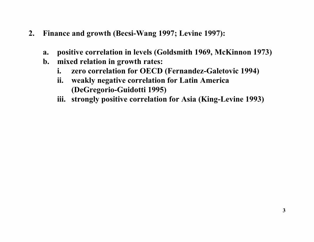
2. Finance and growth (Becsi-Wang 1997; Levine 1997):

a. positive correlation in levels (Goldsmith 1969, McKinnon 1973)b. mixed relation in growth rates:

i. zero correlation for OECD (Fernandez-Galetovic 1994)ii. weakly negative correlation for Latin America

(DeGregorio-Guidotti 1995) iii. strongly positive correlation for Asia (King-Levine 1993)

3

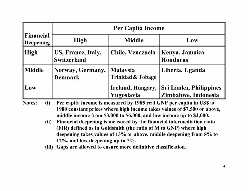
FinancialDeepening

Per Capita Income

High Middle Low

High US, France, Italy,Switzerland

Chile, Venezuela Kenya, JamaicaHonduras

Middle Norway, Germany,Denmark

MalaysiaTrinidad & Tobago

Liberia, Uganda

Low Ireland, Hungary,Yugoslavia

Sri Lanka, PhilippinesZimbabwe, Indonesia

Notes: (i) Per capita income is measured by 1985 real GNP per capita in US$ at1980 constant prices where high income takes values of $7,500 or above,middle income from $3,000 to $6,000, and low income up to $2,000.

(ii) Financial deepening is measured by the financial intermediation ratio(FIR) defined as in Goldsmith (the ratio of M to GNP) where highdeepening takes values of 13% or above, middle deepening from 8% to12%, and low deepening up to 7%.

(iii) Gaps are allowed to ensure more definitive classification.

4

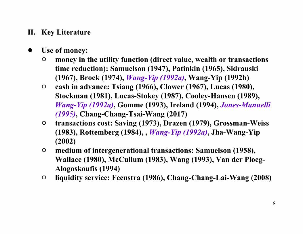
II. Key Literature

! Use of money: " money in the utility function (direct value, wealth or transactions

time reduction): Samuelson (1947), Patinkin (1965), Sidrauski(1967), Brock (1974), Wang-Yip (1992a), Wang-Yip (1992b)

" cash in advance: Tsiang (1966), Clower (1967), Lucas (1980),Stockman (1981), Lucas-Stokey (1987), Cooley-Hansen (1989),Wang-Yip (1992a), Gomme (1993), Ireland (1994), Jones-Manuelli(1995), Chang-Chang-Tsai-Wang (2017)

" transactions cost: Saving (1973), Drazen (1979), Grossman-Weiss(1983), Rottemberg (1984), , Wang-Yip (1992a), Jha-Wang-Yip(2002)

" medium of intergenerational transactions: Samuelson (1958),Wallace (1980), McCullum (1983), Wang (1993), Van der Ploeg-Alogoskoufis (1994)

" liquidity service: Feenstra (1986), Chang-Chang-Lai-Wang (2008)

5

" money and search: Wicksell (1898), Jones (1976), Wang (1987),Kiyotaki-Wright (1989, 1993), Trejos-Wrigth (1995), Lagos-Wright (2002), Laing-Li-Wang (2007, 2013)

! Major Roles of Financial Intermediation: " liquidity management: Diamond-Dybvig (1993),

Bencinvinga-Smith (1991)" risk pooling: Townsend (1978), Greenwood-Jovanovic (1990),

Bencivenga-Smith (1993)" productive loan services: Tssidon (1992), Aghion-Bolton (1997)" effective monitoring: Williamson (1986), Greenwood-Jovanovic

(1990), and the literature on:- borrowing/collateral/pledgeability constraints- venture capitalism- micro finance

" funds pooling: Besley (1994), Becsi-Wang-Wynne (1999), and theliterature on micro finance

6

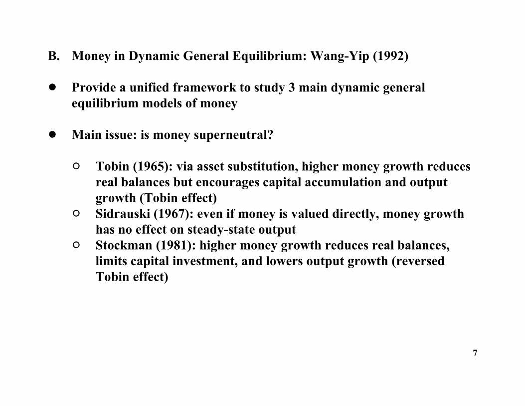
B. Money in Dynamic General Equilibrium: Wang-Yip (1992)

! Provide a unified framework to study 3 main dynamic generalequilibrium models of money

! Main issue: is money superneutral?

" Tobin (1965): via asset substitution, higher money growth reducesreal balances but encourages capital accumulation and outputgrowth (Tobin effect)

" Sidrauski (1967): even if money is valued directly, money growthhas no effect on steady-state output

" Stockman (1981): higher money growth reduces real balances,limits capital investment, and lowers output growth (reversedTobin effect)

7

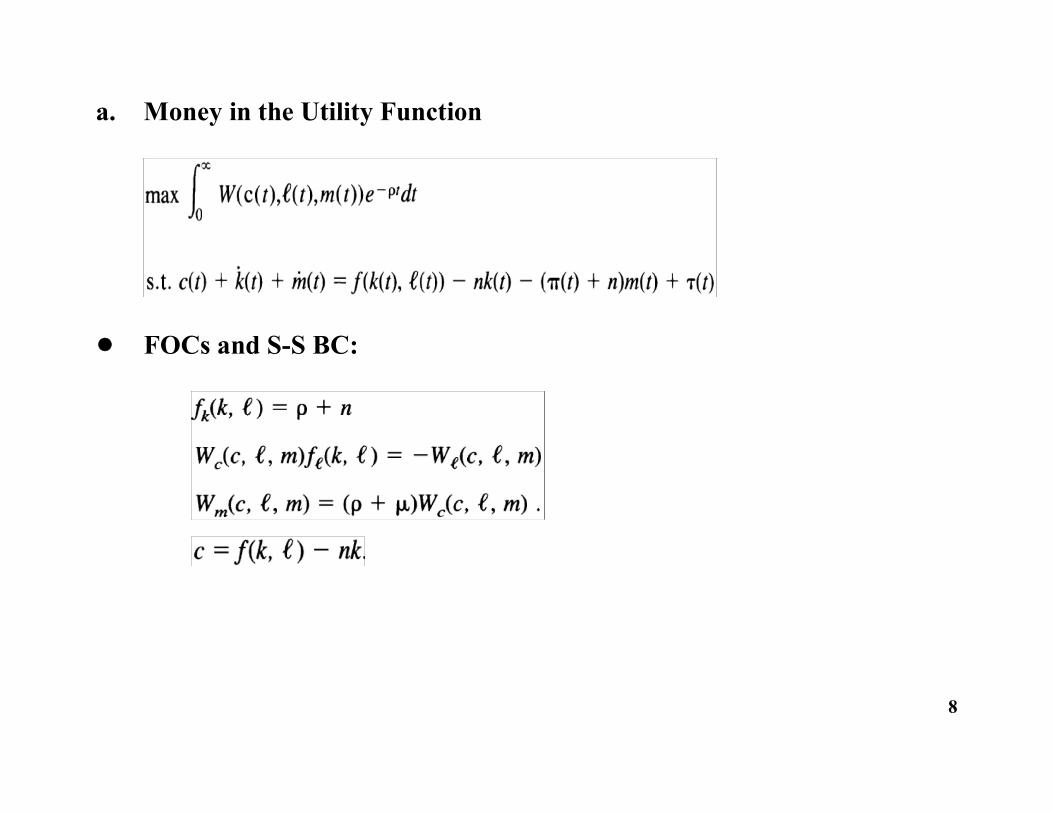
a. Money in the Utility Function

! FOCs and S-S BC:

8

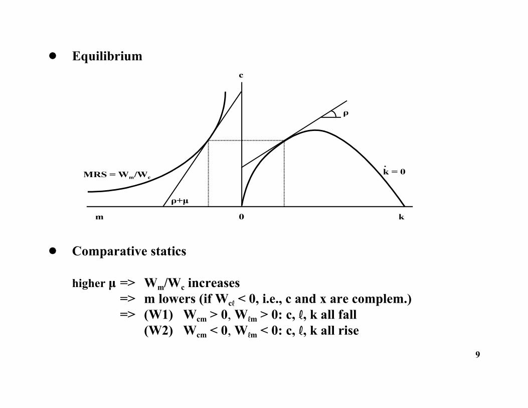
! Equilibrium

! Comparative statics

higher μ => Wm/Wc increases=> m lowers (if Wc < 0, i.e., c and x are complem.)=> (W1) Wcm > 0, Wm > 0: c, , k all fall

(W2) Wcm < 0, Wm < 0: c, , k all rise

9

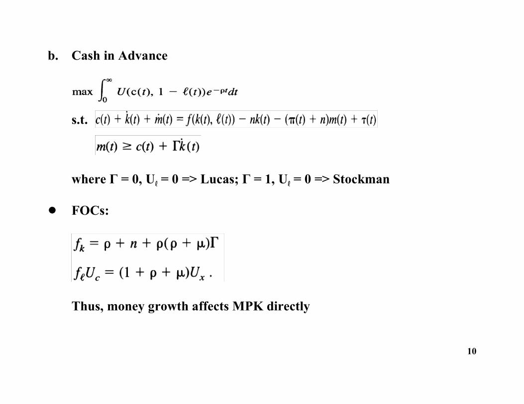
b. Cash in Advance

s.t.

where Γ = 0, U = 0 => Lucas; Γ = 1, U = 0 => Stockman

! FOCs:

Thus, money growth affects MPK directly

10

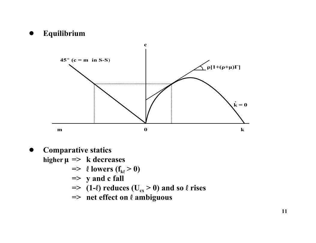
! Equilibrium

! Comparative staticshigher μ => k decreases

=> lowers (fk > 0)=> y and c fall => (1-) reduces (Ucx > 0) and so rises=> net effect on ambiguous

11

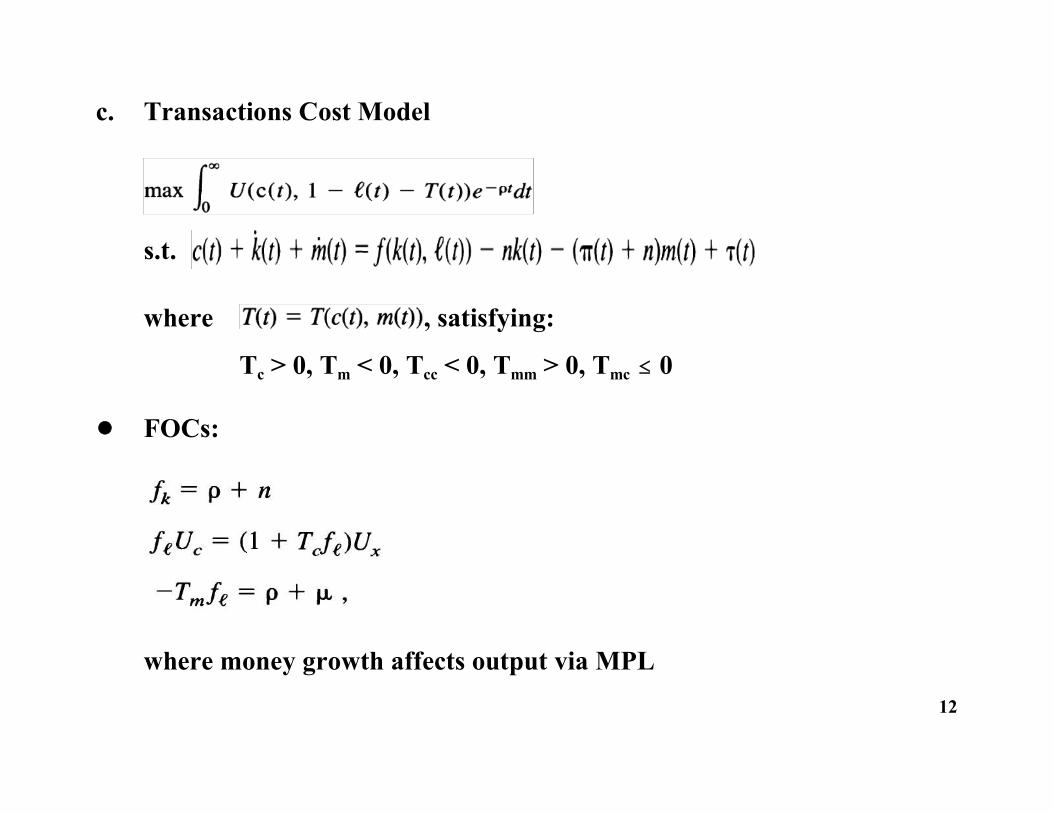
c. Transactions Cost Model

s.t.

where , satisfying:

Tc > 0, Tm < 0, Tcc < 0, Tmm > 0, Tmc 0

! FOCs:

where money growth affects output via MPL12

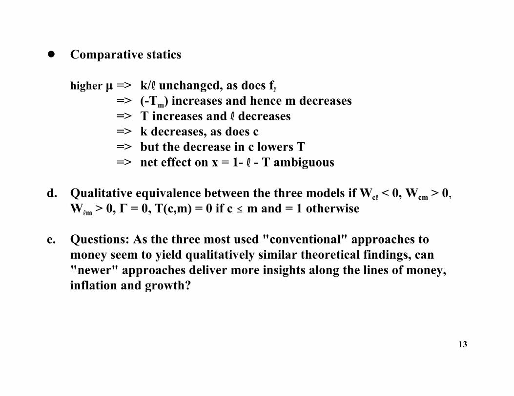
! Comparative statics

higher μ => k/ unchanged, as does f => (-Tm) increases and hence m decreases

=> T increases and decreases=> k decreases, as does c=> but the decrease in c lowers T=> net effect on x = 1- - T ambiguous

d. Qualitative equivalence between the three models if Wc < 0, Wcm > 0,Wm > 0, Γ = 0, T(c,m) = 0 if c m and = 1 otherwise

e. Questions: As the three most used "conventional" approaches tomoney seem to yield qualitatively similar theoretical findings, can"newer" approaches deliver more insights along the lines of money,inflation and growth?

13

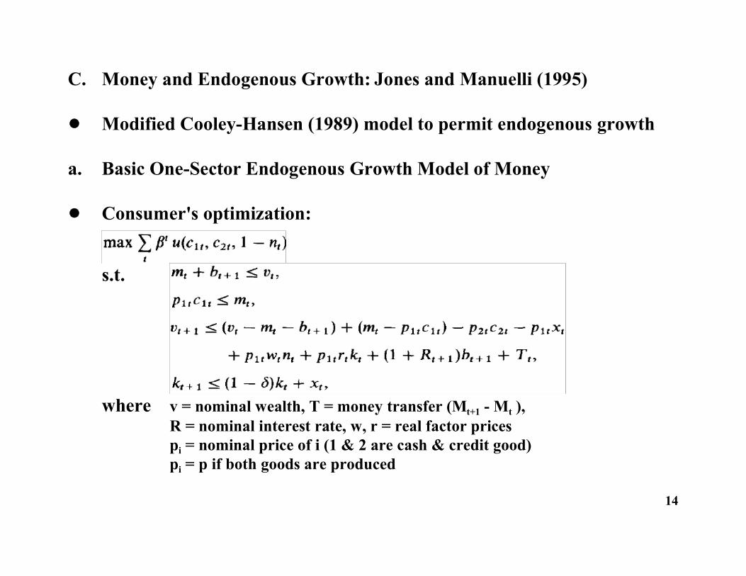
C. Money and Endogenous Growth: Jones and Manuelli (1995)

! Modified Cooley-Hansen (1989) model to permit endogenous growth

a. Basic One-Sector Endogenous Growth Model of Money

! Consumer's optimization:

s.t.

where v = nominal wealth, T = money transfer (Mt+1 - Mt ), R = nominal interest rate, w, r = real factor pricespi = nominal price of i (1 & 2 are cash & credit good)pi = p if both goods are produced

14

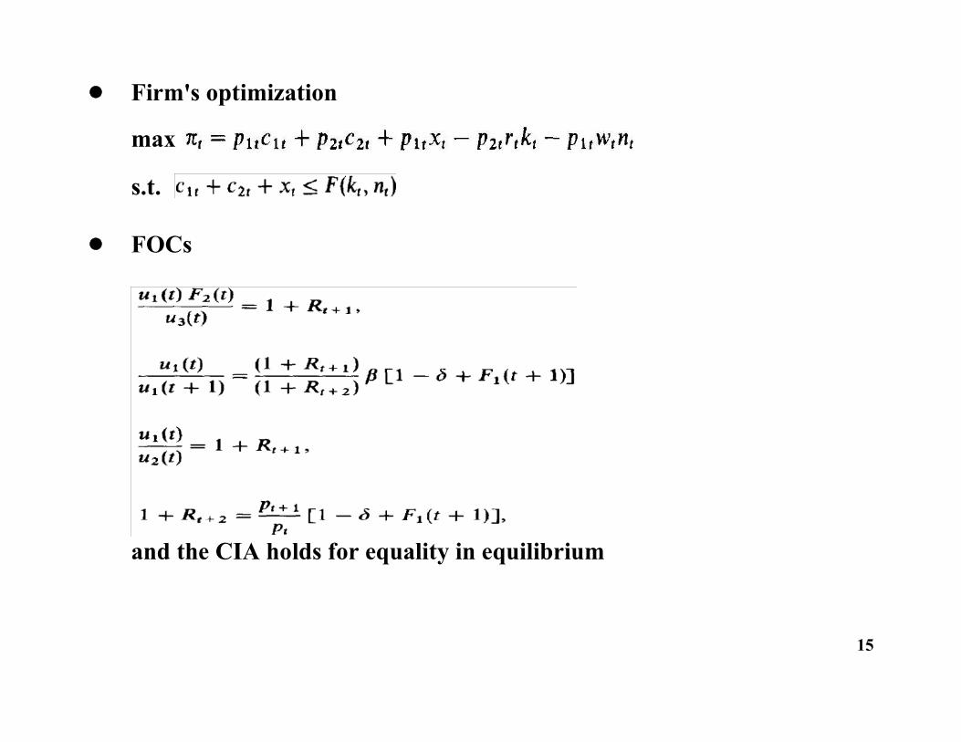
! Firm's optimization

max

s.t.

! FOCs

and the CIA holds for equality in equilibrium

15

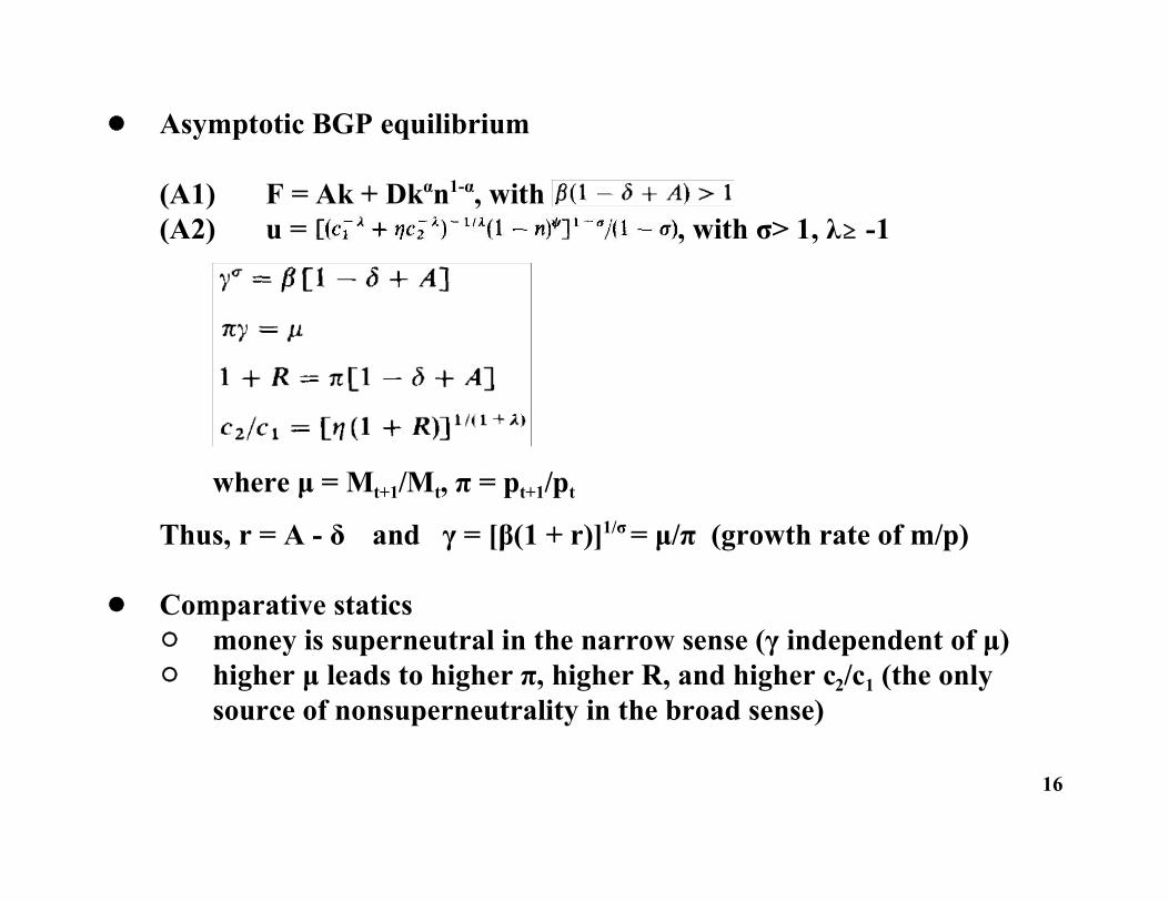
! Asymptotic BGP equilibrium

(A1) F = Ak + Dkαn1-α, with (A2) u = , with σ> 1, λ -1

where μ = Mt+1/Mt, π = pt+1/pt

Thus, r = A - δ and γ = [β(1 + r)]1/σ = μ/π (growth rate of m/p)

! Comparative statics" money is superneutral in the narrow sense (γ independent of μ)" higher μ leads to higher π, higher R, and higher c2/c1 (the only

source of nonsuperneutrality in the broad sense)

16

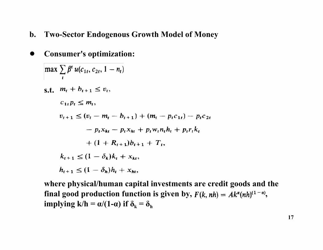
b. Two-Sector Endogenous Growth Model of Money

! Consumer's optimization:

s.t.

where physical/human capital investments are credit goods and thefinal good production function is given by, ,implying k/h = α/(1-α) if δk = δh

17

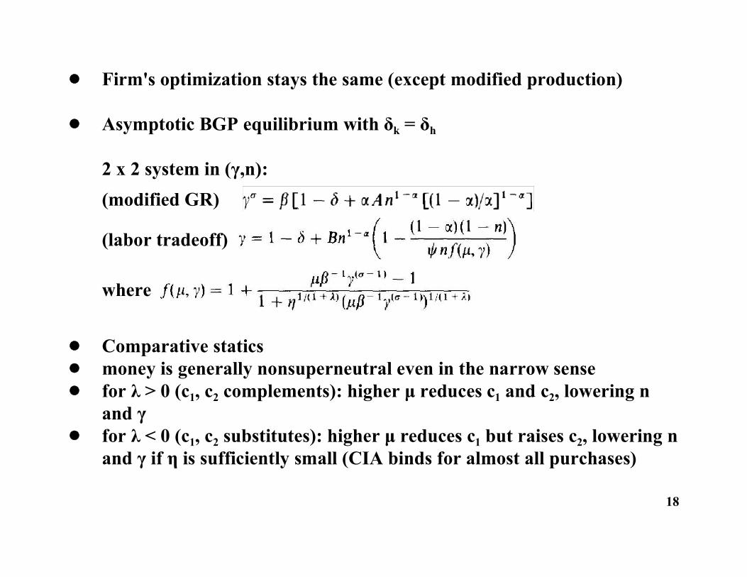
! Firm's optimization stays the same (except modified production)

! Asymptotic BGP equilibrium with δk = δh

2 x 2 system in (γ,n):(modified GR)

(labor tradeoff)

where

! Comparative statics! money is generally nonsuperneutral even in the narrow sense! for λ > 0 (c1, c2 complements): higher μ reduces c1 and c2, lowering n

and γ! for λ < 0 (c1, c2 substitutes): higher μ reduces c1 but raises c2, lowering n

and γ if η is sufficiently small (CIA binds for almost all purchases)

18

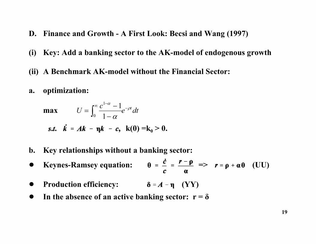
D. Finance and Growth - A First Look: Becsi and Wang (1997)

(i) Key: Add a banking sector to the AK-model of endogenous growth

(ii) A Benchmark AK-model without the Financial Sector:

a. optimization:

max U c e dtt

1

0

11

k(0) =k0 > 0.

b. Key relationships without a banking sector:

! Keynes-Ramsey equation: => (UU)

! Production efficiency: (YY)! In the absence of an active banking sector: r = δ

19

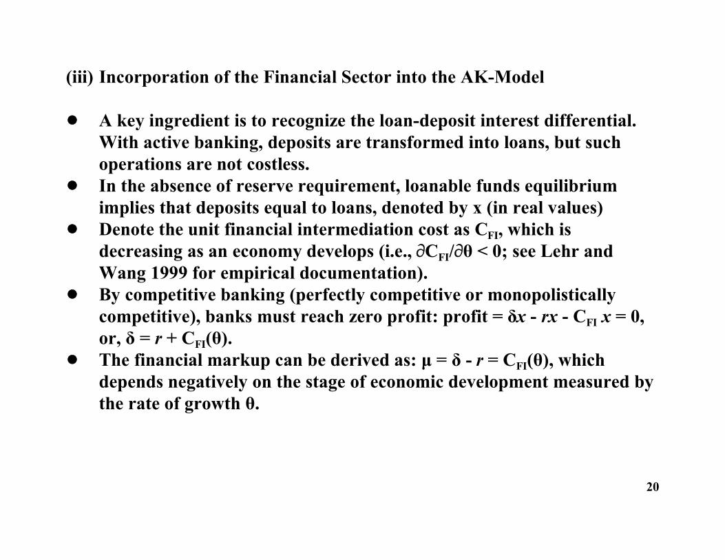
(iii) Incorporation of the Financial Sector into the AK-Model

! A key ingredient is to recognize the loan-deposit interest differential. With active banking, deposits are transformed into loans, but suchoperations are not costless.

! In the absence of reserve requirement, loanable funds equilibriumimplies that deposits equal to loans, denoted by x (in real values)

! Denote the unit financial intermediation cost as CFI, which isdecreasing as an economy develops (i.e., CFI/θ < 0; see Lehr andWang 1999 for empirical documentation).

! By competitive banking (perfectly competitive or monopolisticallycompetitive), banks must reach zero profit: profit = δx - rx - CFI x = 0,or, δ = r + CFI(θ).

! The financial markup can be derived as: μ = δ - r = CFI(θ), whichdepends negatively on the stage of economic development measured bythe rate of growth θ.

20

21

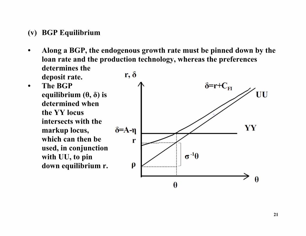
(v) BGP Equilibrium • Along a BGP, the endogenous growth rate must be pinned down by the

loan rate and the production technology, whereas the preferences determines the deposit rate.

• The BGP equilibrium (θ, δ) is determined when the YY locus intersects with the markup locus, which can then be used, in conjunction with UU, to pin down equilibrium r.

! Comparative statics:" production innovation: A => δ , r , μ , θ " banking innovation: exog. CFI => δ unchanged, r , μ , θ " annuity innovation: ρ => δ, θ , r , μ " effective monitoring: A and CFI => δ , r , μ , θ " technological and annuity innovation: A and ρ => δ , r ? (

if direct effect dominates), μ , θ " limited bank entry: more local market power => μ , θ ? (Smith

vs. Schumpeter)

22

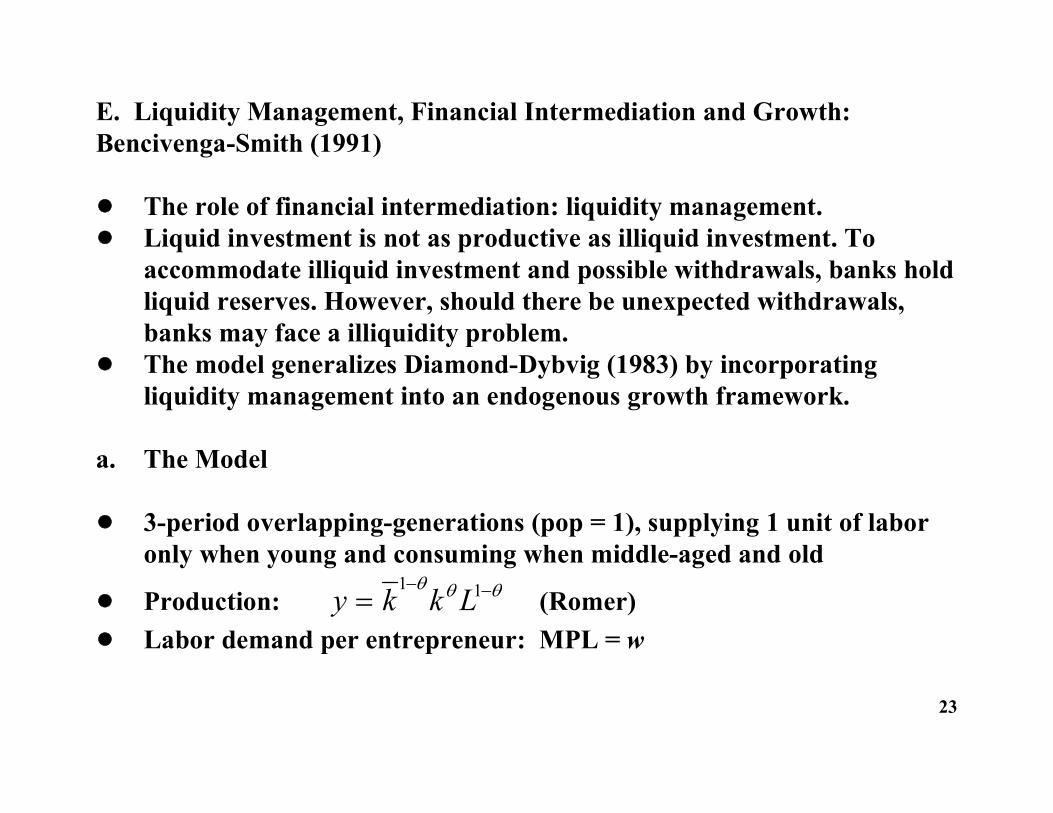
E. Liquidity Management, Financial Intermediation and Growth:Bencivenga-Smith (1991)

! The role of financial intermediation: liquidity management. ! Liquid investment is not as productive as illiquid investment. To

accommodate illiquid investment and possible withdrawals, banks holdliquid reserves. However, should there be unexpected withdrawals,banks may face a illiquidity problem.

! The model generalizes Diamond-Dybvig (1983) by incorporatingliquidity management into an endogenous growth framework.

a. The Model

! 3-period overlapping-generations (pop = 1), supplying 1 unit of laboronly when young and consuming when middle-aged and old

! Production: (Romer)y k k L 1 1

! Labor demand per entrepreneur: MPL = w

23

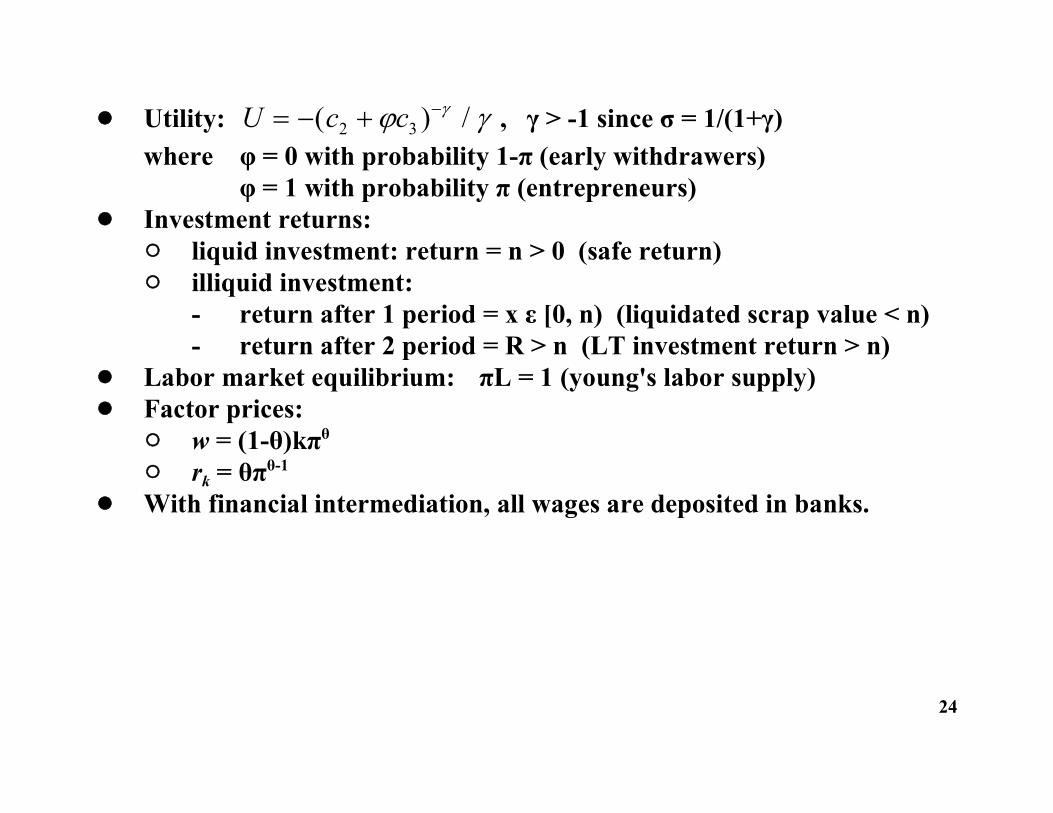
! Utility: , γ > -1 since σ = 1/(1+γ)U c c ( ) /2 3

where φ = 0 with probability 1-π (early withdrawers)φ = 1 with probability π (entrepreneurs)

! Investment returns:" liquid investment: return = n > 0 (safe return)" illiquid investment:

- return after 1 period = x ε [0, n) (liquidated scrap value < n)- return after 2 period = R > n (LT investment return > n)

! Labor market equilibrium: πL = 1 (young's labor supply)! Factor prices:

" w = (1-θ)kπθ

" rk = θπθ-1

! With financial intermediation, all wages are deposited in banks.

24

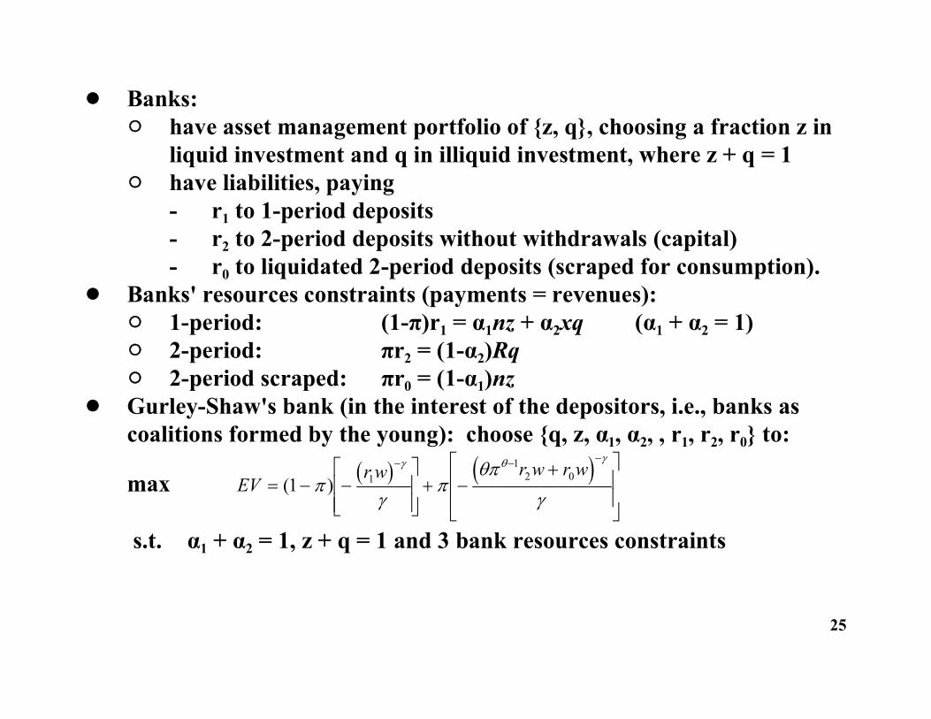
! Banks: " have asset management portfolio of {z, q}, choosing a fraction z in

liquid investment and q in illiquid investment, where z + q = 1" have liabilities, paying

- r1 to 1-period deposits- r2 to 2-period deposits without withdrawals (capital)- r0 to liquidated 2-period deposits (scraped for consumption).

! Banks' resources constraints (payments = revenues):" 1-period: (1-π)r1 = α1nz + α2xq (α1 + α2 = 1)" 2-period: πr2 = (1-α2)Rq" 2-period scraped: πr0 = (1-α1)nz

! Gurley-Shaw's bank (in the interest of the depositors, i.e., banks ascoalitions formed by the young): choose {q, z, α1, α2, , r1, r2, r0} to:

max EV

r w r w r w

( )1 11

2 0

s.t. α1 + α2 = 1, z + q = 1 and 3 bank resources constraints

25

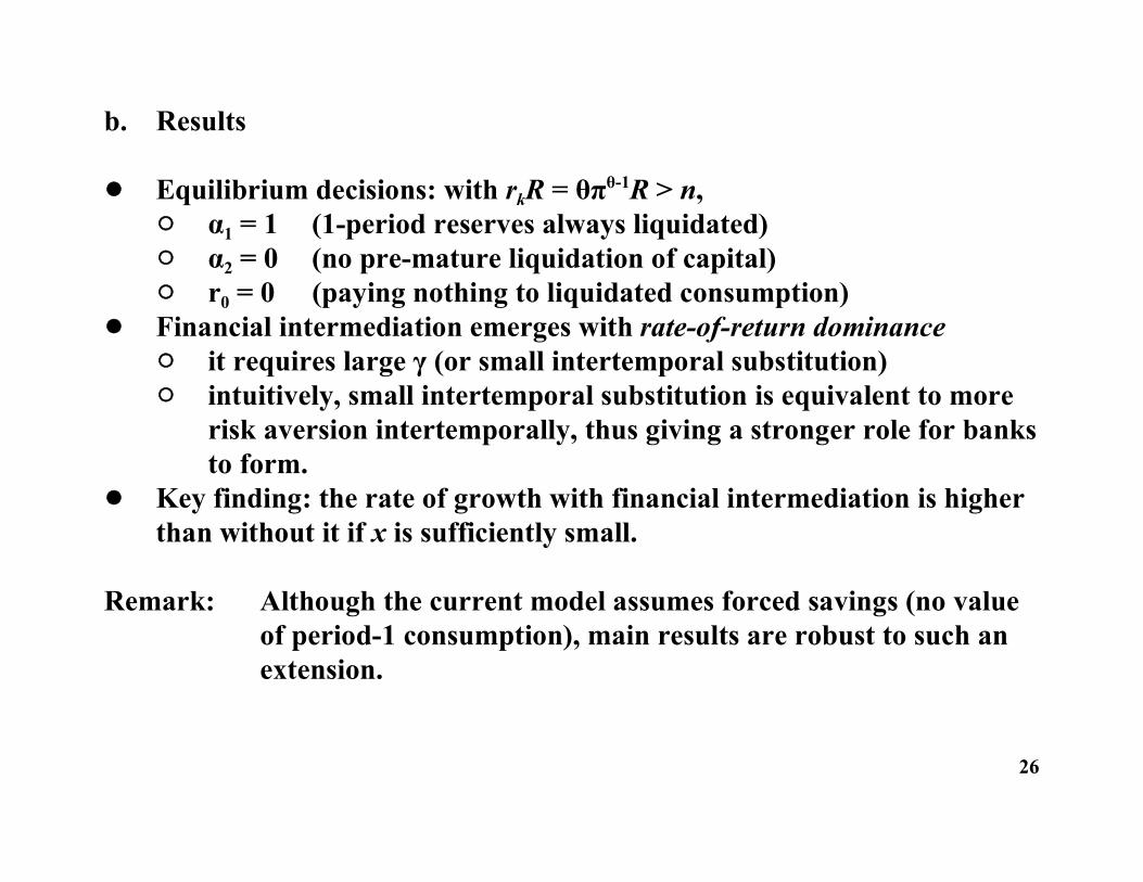
b. Results

! Equilibrium decisions: with rkR = θπθ-1R > n," α1 = 1 (1-period reserves always liquidated)" α2 = 0 (no pre-mature liquidation of capital)" r0 = 0 (paying nothing to liquidated consumption)

! Financial intermediation emerges with rate-of-return dominance" it requires large γ (or small intertemporal substitution) " intuitively, small intertemporal substitution is equivalent to more

risk aversion intertemporally, thus giving a stronger role for banksto form.

! Key finding: the rate of growth with financial intermediation is higherthan without it if x is sufficiently small.

Remark: Although the current model assumes forced savings (no valueof period-1 consumption), main results are robust to such anextension.

26

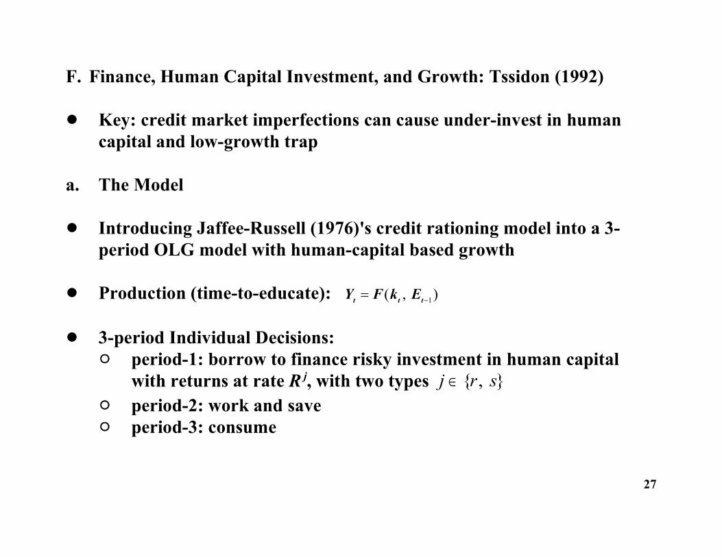
F. Finance, Human Capital Investment, and Growth: Tssidon (1992)

! Key: credit market imperfections can cause under-invest in humancapital and low-growth trap

a. The Model

! Introducing Jaffee-Russell (1976)'s credit rationing model into a 3-period OLG model with human-capital based growth

! Production (time-to-educate): Y F k Et t t ( , )1

! 3-period Individual Decisions:" period-1: borrow to finance risky investment in human capital

with returns at rate R j, with two types j r s { , }" period-2: work and save" period-3: consume

27

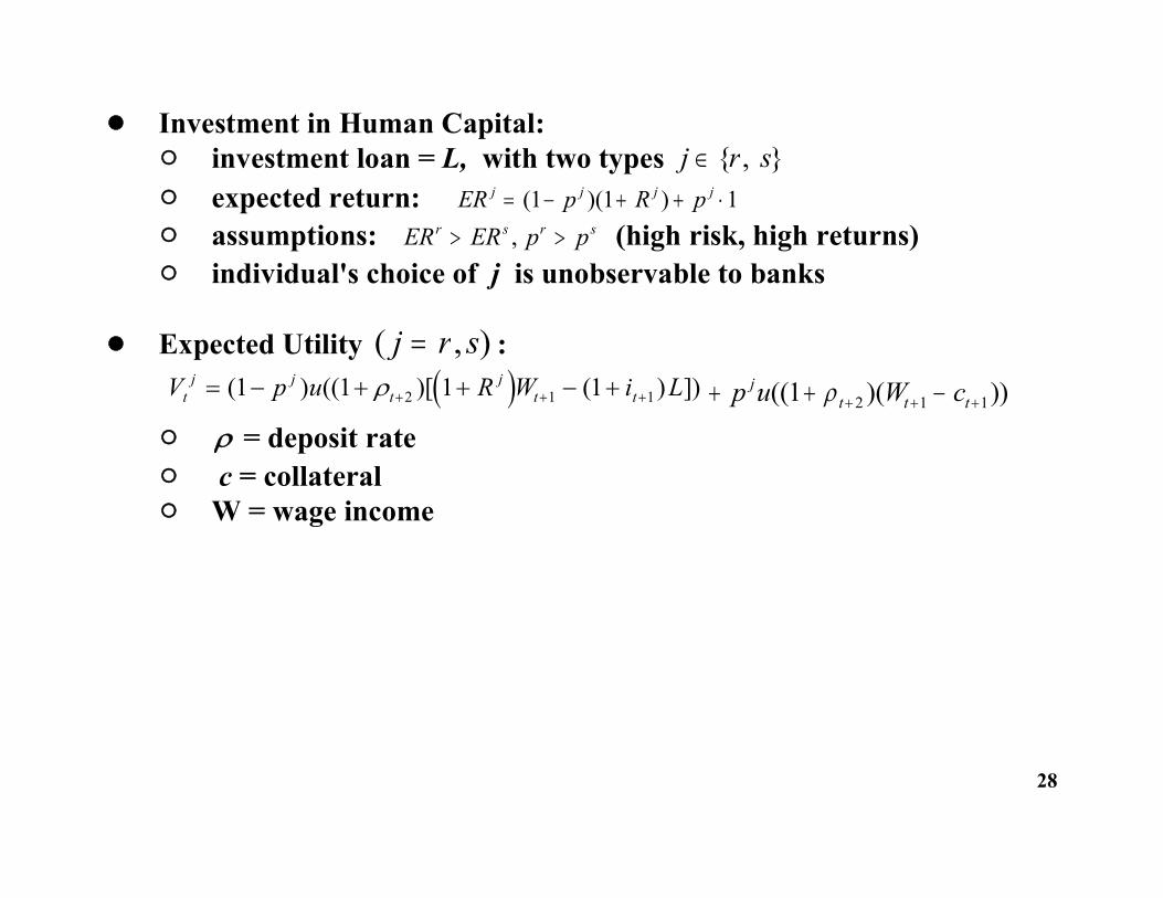
! Investment in Human Capital:" investment loan = L, with two types j r s { , }" expected return: ER p R pj j j j ( )( )1 1 1" assumptions: (high risk, high returns)ER ER p pr s r s , " individual's choice of j is unobservable to banks

! Expected Utility :( , )j r s V p u R W i Lt

j jt

jt t ( ) (( )[ ( ) ])1 1 1 12 1 1 p u W cj

t t t(( )( ))1 2 1 1

" = deposit rate" c = collateral" W = wage income

28

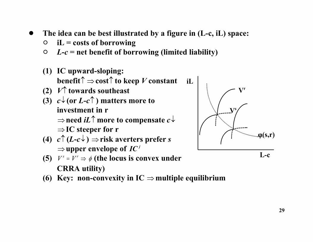
! The idea can be best illustrated by a figure in (L-c, iL) space:" iL = costs of borrowing" L-c = net benefit of borrowing (limited liability)

(1) IC upward-sloping: benefit cost to keep V constant

(2) V towards southeast(3) c (or L-c ) matters more to

investment in rneed iL more to compensate c IC steeper for r

(4) c (L-c ) risk averters prefer s upper envelope of IC j

(5) (the locus is convex underV Vs r CRRA utility)

(6) Key: non-convexity in IC multiple equilibrium

29

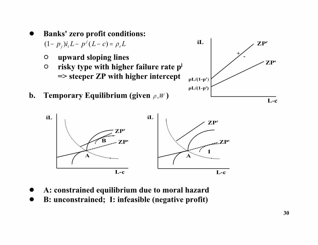
! Banks' zero profit conditions: ( ) ( )1 p i L p L c Lj t

jt

" upward sloping lines" risky type with higher failure rate pj

=> steeper ZP with higher intercept

b. Temporary Equilibrium (given ) ,W

! A: constrained equilibrium due to moral hazard! B: unconstrained; I: infeasible (negative profit)

30

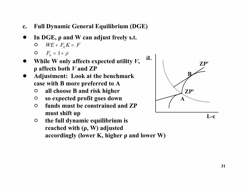
c. Full Dynamic General Equilibrium (DGE)

! In DGE, ρ and W can adjust freely s.t." WE F K Fk " Fk 1

! While W only affects expected utility V,ρ affects both V and ZP

! Adjustment: Look at the benchmarkcase with B more preferred to A" all choose B and risk higher" so expected profit goes down " funds must be constrained and ZP

must shift up" the full dynamic equilibrium is

reached with (ρ, W) adjustedaccordingly (lower K, higher ρ and lower W)

31

d. Main Findings

! Moral hazard credit rationing equilibrium at A: " low human capital" low MPK (or )" low-growth trap

! Policy Prescription:" provision of education loans with better monitoring or law

enforcement" this will reduce moral hazard problems, thus promoting

investment in high risk but high return higher education" as a result, it enhances economic growth, avoiding the low human

capital-low growth trap

32

G. Finance, Investment, and Growth: Aghion-Bolton (1997)

! The Aghion-Bolton model can be regarded as an extension of Baneree-Newman (1993) by allowing full dynamics of wealth evolution with:(i) endogenous occupational choice (ii) credit market imperfections(iii) nonstationary distribution (cf. Hopenhyne-Prescott)

33

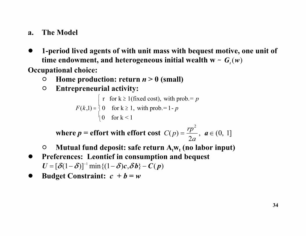
a. The Model

! 1-period lived agents of with unit mass with bequest motive, one unit oftime endowment, and heterogeneous initial wealth w G wt ( )

Occupational choice:" Home production: return n > 0 (small)" Entrepreneurial activity:

F kp

p( , )1 00

r for k 1(fixed cost), with prob.= for k 1, with prob.= 1- for k < 1

where p = effort with effort cost C p rpa

( ) ,2

2a ( , ]0 1

" Mutual fund deposit: safe return Atwt (no labor input)! Preferences: Leontief in consumption and bequest

U c b C p [ ( )] min{( ) , } ( ) 1 11

! Budget Constraint: c + b = w

34

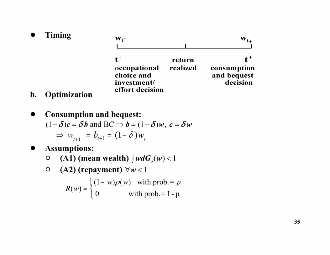
! Timing

b. Optimization

! Consumption and bequest: ( ) ( ) ,1 1 c b b w c w and BC

w b wt t t1 1 1( )

! Assumptions:" (A1) (mean wealth) wdG w0 1( ) " (A2) (repayment) w 1

R ww w p

( )( ) ( )

10

with prob.= with prob.= 1- p

35

! Occupational choice and investment decision: " Potential borrower (w <1): maxp

implying

" Rich lender : maxp implying ( )w 1

36

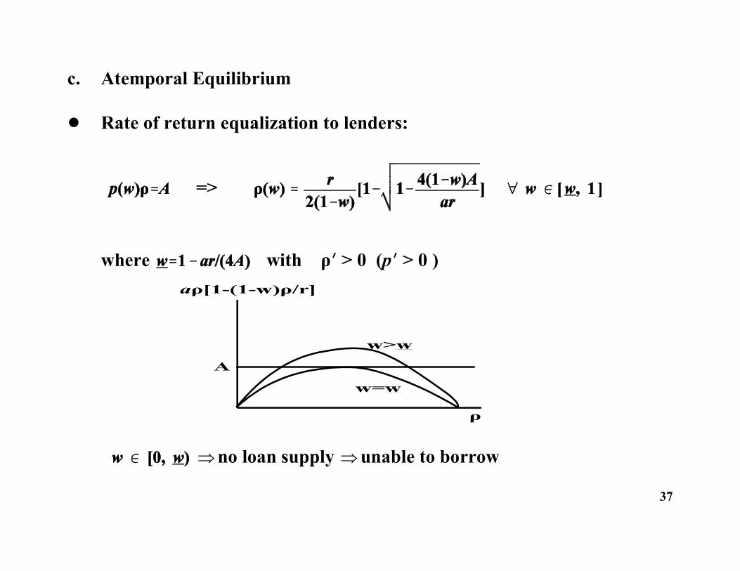
c. Atemporal Equilibrium

! Rate of return equalization to lenders:

=>

where with ρ > 0 (p > 0 )

no loan supply unable to borrow

37

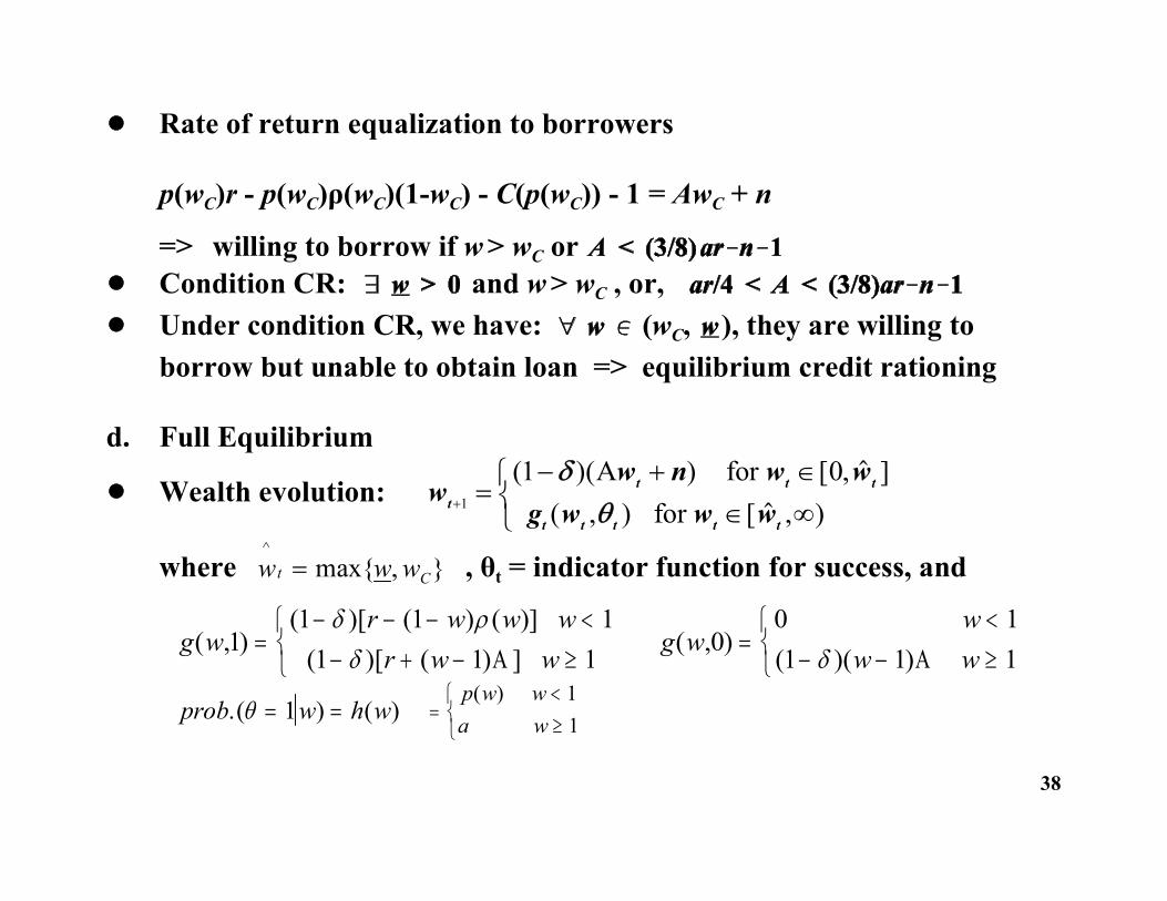
! Rate of return equalization to borrowers

p(wC)r - p(wC)ρ(wC)(1-wC) - C(p(wC)) - 1 = AwC + n

=> willing to borrow if w > wC or ! Condition CR: and w > wC , or, ! Under condition CR, we have: (wC, ), they are willing to

borrow but unable to obtain loan => equilibrium credit rationing

d. Full Equilibrium

! Wealth evolution: ww n w w

g w w wtt t t

t t t t t

1

1 0( )( ) [ , ]( , )

for

for [ , )

where , θt = indicator function for success, andw w wt C

^max{ , }

g wr w w wr w w( , )

( )[ ( ) ( )]( )[ ( ) ]1

1 1 11 1

1

g ww

w w( , ) ( )( )00 11 1 1

prob w h w.( ) ( ) 1

p w wa w

( ) 11

38

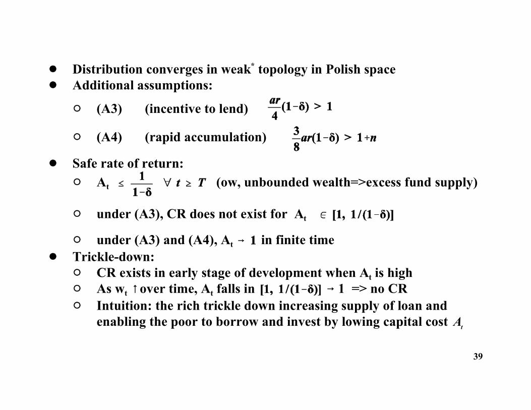
! Distribution converges in weak* topology in Polish space! Additional assumptions:

" (A3) (incentive to lend)

" (A4) (rapid accumulation)

! Safe rate of return: " At (ow, unbounded wealth=>excess fund supply)

" under (A3), CR does not exist for At

" under (A3) and (A4), At in finite time ! Trickle-down:

" CR exists in early stage of development when At is high" As wt over time, At falls in 1 => no CR" Intuition: the rich trickle down increasing supply of loan and

enabling the poor to borrow and invest by lowing capital cost At

39