Embed Size (px)
Citation preview

MOLECULAR MODELING OF PROTEINS AND MATHEMATICALPREDICTION OF PROTEIN STRUCTURE
ARNOLD NEUMAIER ∗
Abstract. This paper discusses the mathematical formulation of and solution attempts for theso-called protein folding problem. The static aspect is concerned with how to predict the folded(native, tertiary) structure of a protein, given its sequence of amino acids. The dynamic aspect asksabout the possible pathways to folding and unfolding, including the stability of the folded protein.
From a mathematical point of view, there are several main sides to the static problem:– the selection of an appropriate potential energy function;– the parameter identification by fitting to experimental data; and– the global optimization of the potential.The dynamic problem entails, in addition, the solution of (because of multiple time scales very
stiff) ordinary or stochastic differential equations (molecular dynamics simulation), or (in case ofconstrained molecular dynamics) of differential-algebraic equations. A theme connecting the staticand dynamic aspect is the determination and formation of secondary structure motifs.
The present paper gives a self-contained introduction to the necessary background from physicsand chemistry and surveys some of the literature. It also discusses the various mathematical problemsarising, some deficiencies of the current models and algorithms, and possible (past and future) attacksto arrive at solutions to the protein folding problem.
Key words. protein folding, molecular mechanics, transition states, stochastic differentialequations, dynamic energy minimization, harmonic approximation, multiple time scales, stiffness,differential-algebraic equation, molecular dynamics simulations, potential energy surface, parameterestimation, conformational entropy, secondary structure, tertiary structure, native structure, confor-mational entropy, global optimization, simulated annealing, genetic algorithm, smoothing method,diffusion equation method, branch and bound, backbone potential models, lattice models, contactpotential, threading, solvation energy, combination rule
AMS subject classifications. primary 92C40; secondary 65L05, 90C26
1. Introduction. It is God’s privilege to conceal things,but the kings’ pride is to research them.(Proverbs 25:2; ascribed to KingSolomon of Israel, ca. 1000 B.C.)
This paper is the result of my investigations into the problems involved in themathematical prediction of (tertiary, 3-dimensional) protein structure given the (pri-mary, linear) structure defined by the sequence of amino acids of the protein. Thisso-called protein folding problem is one of the most challenging problems in current bio-chemistry, and is a very rich source of interesting problems in mathematical modelingand numerical analysis, requiring an interplay of techniques in eigenvalue calculations,stiff differential equations, stochastic differential equations, local and global optimiza-tion, nonlinear least squares, multidimensional approximation of functions, design ofexperiment, and statistical classification of data. Even topological concepts like theMorse index (Mezey [205]) and invariants in knot theory (Jones polynomials) havebeen discussed in this context; see, e.g., Sumners [311]. An extensive recent report[218] from the U.S. National Research Council on the mathematical challenges fromtheoretical and computational chemistry shows the protein folding problem embeddedinto a large variety of other mathematical challenges in chemistry.
The aims of the present paper are to introduce mathematicians to the subject,to provide enough background that the problems in the mathematical modeling of
∗ Institut fur Mathematik, Universitat Wien, Strudlhofgasse 4, A-1090 Wien, Austria.email: [email protected] WWW: http://solon.cma.univie.ac.at/∼neum/
1

2 A. NEUMAIER
proteins become transparent, to expose the merits and deficiencies of current models,to describe the numerical difficulties in structure prediction when a model is speci-fied, and to point out possible ways of improving model formulation and predictiontechniques.
Molecular biology is mankind’s attempt to figure out how God engineered Hisgreatest invention – life. As with all great inventions, details are top secret; however,even top secrets may become known. I find it a great privilege to live in a time whereGod allows us to gain some insight into His construction plans, only a short step awayfrom giving us the power to control life processes genetically. I hope it will be to thebenefit of mankind, and not to its destruction.
After the successful deciphering of the genetic code that defines how the aminoacid sequences of proteins are coded in the DNA, one of the major missing steps inunderstanding the chemical basis of life is the protein folding problem: the task ofunderstanding and predicting how the information coded in the amino acid sequenceof proteins at the time of their formation translates into the 3-dimensional structure ofthe biologically active protein. (Actually, there are also folding problems in connectionwith nucleotide sequences in DNA and RNA, but this survey is limited to proteinfolding only. For the mathematics of nuclein acids and genome analysis see, e.g., arecent U.S. National Research Council report by Lander & Waterman [178].)
Proteins are the machines and building blocks of living cells. If we compare aliving body to our world, each cell corresponds to a town, and the proteins are thehouses, bridges, cars, cranes, roads, airplanes, etc. There are huge numbers of differentproteins, each one performing its specific task.
Since it is known already how to use genetic engineering to produce proteins witha given amino acid sequence, knowledge of how such a protein would fold would allowone to predict its chemical and biological properties. If we were able to solve theprotein folding problem, it would greatly simplify the tasks of interpreting the datacollected by the human genome project, understanding the mechanism of hereditaryand infectuous diseases, designing drugs with specific therapeutical properties (see,e.g., Balbes et al. [12]), and of growing biological polymers with specific materialproperties.
The literature on the various aspects of protein folding is enormous, and I madeno attempt of being complete in the coverage of papers; instead I simply quote thepapers that I have found useful in the preparation of this study. Given the currentamount of activity in this broad field and my own time limitations, it is probablyinevitable that I also omitted one or the other recent paper with new developments,and I’d appreciate being informed about any serious omissions.
However, I tried to draw a complete picture of the physical and chemical back-ground needed to understand modeling details and to be able to read more special-ized literature. To allow an assessment of the approximations made in the traditionalmodeling process and to aid investigations in other molecular modeling problems notdirectly related to protein folding, I also included (less complete) remarks and point-ers to the literature regarding attempts of more detailed or accurate modeling (e.g.,quantum corrections) even if these are (in the near future) unlikely to be relevant topractical calculations with macromolecules. Thus the paper can also be viewed as acase study in mathematical modeling of a complex scientific problem.
For further information, we refer to the introductory paper Richards [252] inScientific American, to the books by Brooks et al. [34] and Creighton [62], whichcontain thorough treatments of the subject, to the Reviews in Computational Chem-

MOLECULAR MODELING OF PROTEINS 3
istry edited by Lipkowitz & Boyd [191] with many excellent articles on relatedtopics, to the recent survey of Chan & Dill [48], which contains many additionalpointers to the recent literature related to the physics, chemistry and biology of pro-tein folding, and to Pardalos et al. [229] for algorithmic aspects of the optimizationproblems associated with the problem. Two books providing a general background incomputational chemistry are Clark [53] (an introductory overview with little theory)and, more oriented towards biological applications, Warshel [339].
Further useful books on the subject are [30, 34, 44, 110, 138, 253], and anothersurvey, emphasizing the biological aspects, is Jaenicke [156].
More and more, useful material becomes available electronically on the WorldWide Web. At http://solon.cma.univie.ac.at/ neum/protein.html, there is anecessarily biased and incomplete list of links, collected while working on this study.
Acknowledgments. Much of the research necessary for writing this survey wasdone during a year I spent at AT&T Bell Laboratories, Murray Hill.
I’d like to thank David Gay and Margaret Wright for introducing me to thesubject, Frank Stillinger for providing me with background literature and for patientlyanswering my questions, and Tamar Schlick for her many comments on a draft versionof the paper and additional pointers to the literature.
Thanks also go to an anonymous referee who made many suggestions that widenedthe perspective of the survey so that it covers the entire field of protein structure pre-diction; and to Erich Bornberg-Bauer who interpreted the referee’s condensed remarksby providing the literature relevant to meet his requests, and who produced most ofthe figures.
2. Proteins. Chemical structure. From a purely chemical point of view, aprotein is simply a polymer consisting of a long chain of amino acid residues. Moreprecisely, polymers of this type are called di-, tri-, oligo-, or polypeptides if they consistof 2, 3, several, or many residues, respectively. Each amino acid (except proline) hasthe structure given in Figure 1, where R stands for the side chain characteristic forspecific amino acids.
αH N C C O H
R
H H O
Fig. 1. An amino acid with side chain R
The proteins in living cells contain 20 different residues, with side chains having1-18 atoms. The residues are usually abbreviated with three identifying letters of thecorresponding amino acid, giving the list
{Ala, Arg, Asn, Asp, Cys, Gln, Glu, Gly, His, Ile,

4 A. NEUMAIER
Leu, Lys, Met, Phe, Pro, Ser, Thr, Trp, Tyr, Val}.
(A set of (ECEPP-)geometries for these amino acids can be found, e.g., in Momanyet al. [210]. For generalities on biochemical nomenclature see [155].
Under the influence of RNA containing the genetic information coding for theamino acid sequence, amino acids polymerize in a specific sequence to a chain withthe structure as given in Figure 2. Bonds joining two residues (called peptide bonds)hydrolize (i.e., break under consumption of a water molecule) in a sufficiently acidenvironment, and this can be used to determine the precise sequence of residues ina given protein. Sometimes, the end groups of a protein, the NH2 amino group andthe COOH carboxyl group, are substituted by other groups; e.g., so-called blockedpolypeptides have CH3 methyl groups at both ends. Since amino acid residues areasymmetric, two distinct proteins correspond to a chain of residues and the chain inreversed order.
amide group H H O R
R H H O
peptide unit
αα
residue residue
i+1
i side chain
side chain
H ... N C C N C C ... O Hpeptide bond
carboxyl group
Fig. 2. The chemical structure of a protein
The repeating –NCαC′– chain of a protein is called its backbone. Although lookinglinear in the diagram displaying the bond structure, interatomic forces bend and twistthe chain in a way characteristic for each protein. They cause the protein molecule tocurl up into a specific three-dimensional geometric configuration called the folded stateof the protein. This configuration and the chemically active groups on the surface ofthe folded protein determine its biological function.
Consequently, biochemists are very keen in wanting to understand how the pri-mary structure (the sequence of the residues) gives rise to the tertiary structure (thefolded state). Intermediate between the two is the secondary structure, i.e., local sys-tematic patterns or motifs like helices, recognizable in shorter pieces of many proteins.The quaternary structure, i.e., the pattern in which proteins crystallize, is less inter-esting from a biological point of view. (The naming reflects the fact that the primarystructure, coded in the cell genome, is the basic information from which the synthe-sis of proteins in a cell proceeds. While folding, secondary structure appears and ismodified until the folded tertiary structure is established; the quaternary structure isthe latest stage, if it is attained at all.)
The smallest proteins, hormones, have about 25 − 100 residues, typical globularproteins about 100−500; fibrous proteins may have more than 3000 residues. Thus thenumber of atoms involved ranges from somewhat less than 500 to more than 10000.One of the smallest proteins, BPTI (bovine pancreatic trypsin inhibitor), with 58

MOLECULAR MODELING OF PROTEINS 5
αβ
x i
x j
x kω
x
p
r
q
Fig. 3. Bond vectors, bond angles, and the dihedral angle
residues and 580 atoms only, has become a well-studied model protein from both thecomputational and the experimental point of view; very accurate data for the crystalstructure are available. Another small protein that has found considerable attentionis Crambin (with 46 residues).
Local geometry. The geometry is captured mathematically by assigning to theith atom a 3-dimensional coordinate vector
xi =
xi1xi2xi3
specifying the position of the atom in space. If two atoms with labels j and k arejoined by a chemical bond, we consider the corresponding bond vector
r = xk − xj ,
with bond length
‖r‖ =√
(r, r),
where
(p, q) := p1q1 + p2q2 + p3q3
is the standard inner product in IR3.Similarly, for two adjacent bonds i-j and k-l, we have the bond vectors
p = xj − xi, q = xl − xk.
The bond angle α =<)(i-j-k) can then be computed from the formulas
cosα =(p, r)
‖p‖‖r‖ , sinα =‖p× r‖‖p‖‖r‖ ,
(together with α ∈ [0o, 180o]), where
p× r =
p2r3 − p3r2
p3r1 − p1r3
p1r2 − p2r1

6 A. NEUMAIER
C N
O
Φ
R
C
H
HR
H
α N C
αC
O
H
peptide bond
ΨΦ
ωΨ
Fig. 4. Backbone dihedral angles of a protein
is the cross product in IR3. The bond angle β =<)(j-k-l) is similarly found from
cosβ =(q, r)
‖q‖‖r‖ , sinβ =‖q × r‖‖q‖‖r‖ .
Finally, the dihedral angle ω =<)(i-j-k-l) ∈ [−180o, 180o] (or the complementarytorsion angle 180o − ω) measures the relative orientation of two adjacent angles in achain i-j-k-l of atoms. It is defined as the angle between the normals through theplanes determined by the atoms i, j, k and j, k, l, respectively, and can be calculatedfrom
cosω =(p× r, r × q)‖p× r‖‖r × q‖ , sinω =
(q × p, r)‖r‖‖p× r‖‖r × q‖ .
In particular, the sign of ω is given by that of the triple product (q × p, r).A full set of bond lengths, bond angles and dihedral angles already fixes the ge-
ometry of a molecule (and often overdetermines it). However, the geometry is quitesensitive to small changes in the angles, and, to reduce the sensitivity, it is usefulto specify in addition a number of so-called out-of-plane bending or improper torsionangles τ =<)(i-j-k-l), that are defined in a similar way for any tetrahedron formedby an atom k with three adjacent atoms i, j, l. Clearly, bond lengths, bond angles,dihedral angles and improper torsion angles are invariant under translation, rotation,and path reversal. However, dihedral and improper torsion angles change sign un-der reflection; their signs therefore model the chirality (left- or right-handedness) ofsubconfigurations.
In a protein, the bond angles are usually denoted by the letter θ, and the dihedralangles describing the torsion around the backbone N–Cα, Cα–C’, and C’–N bonds bythe letters ϕ, ψ and ω, respectively; dihedral angles in the side chain by χ.
Under biological conditions, the bond lengths and bond angles are fairly rigid(with a standard deviation of less than 0.2A for bond lengths and of about 2o forbond angles, see Hendrickson[137]; recent experimental values are reported, e.g., inEngh & Huber [90]). Therefore, the dihedral angles along the backbone (usuallylabeled as in Figure 4) determine the main features of the final geometric shape ofthe folded protein.
Structural information for the proteins with known geometry is collected worldwide in the quickly growing Brookhaven Protein Data Bank (Bernstein [19]), acces-
MOLECULAR MODELING OF PROTEINS 7
sible through the WWW at http://www.pdb.bnl.gov; see also Walsh [338], Stampfet al. [302].
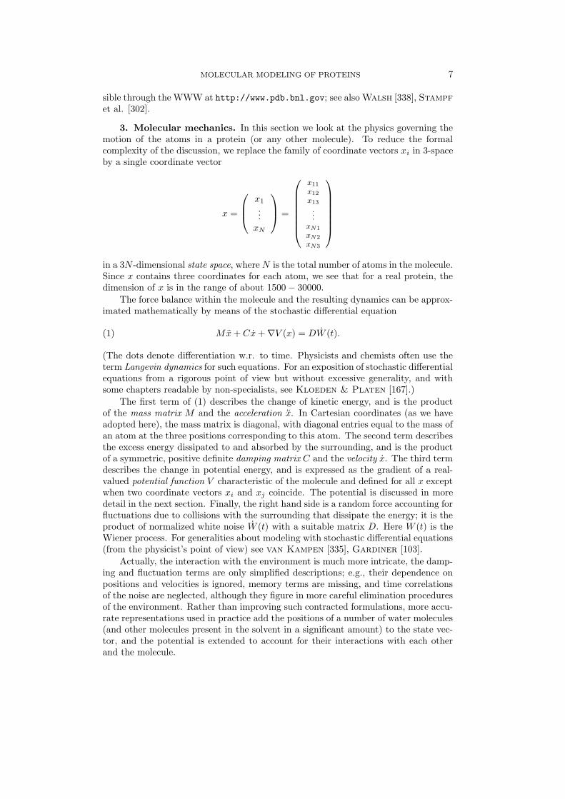
3. Molecular mechanics. In this section we look at the physics governing themotion of the atoms in a protein (or any other molecule). To reduce the formalcomplexity of the discussion, we replace the family of coordinate vectors xi in 3-spaceby a single coordinate vector
x =
x1
...xN
=
x11
x12
x13
.
.
.xN1
xN2
xN3
in a 3N -dimensional state space, where N is the total number of atoms in the molecule.Since x contains three coordinates for each atom, we see that for a real protein, thedimension of x is in the range of about 1500− 30000.
The force balance within the molecule and the resulting dynamics can be approx-imated mathematically by means of the stochastic differential equation
Mx+ Cx+∇V (x) = DW (t).(1)
(The dots denote differentiation w.r. to time. Physicists and chemists often use theterm Langevin dynamics for such equations. For an exposition of stochastic differentialequations from a rigorous point of view but without excessive generality, and withsome chapters readable by non-specialists, see Kloeden & Platen [167].)
The first term of (1) describes the change of kinetic energy, and is the productof the mass matrix M and the acceleration x. In Cartesian coordinates (as we haveadopted here), the mass matrix is diagonal, with diagonal entries equal to the mass ofan atom at the three positions corresponding to this atom. The second term describesthe excess energy dissipated to and absorbed by the surrounding, and is the productof a symmetric, positive definite damping matrix C and the velocity x. The third termdescribes the change in potential energy, and is expressed as the gradient of a real-valued potential function V characteristic of the molecule and defined for all x exceptwhen two coordinate vectors xi and xj coincide. The potential is discussed in moredetail in the next section. Finally, the right hand side is a random force accounting forfluctuations due to collisions with the surrounding that dissipate the energy; it is theproduct of normalized white noise W (t) with a suitable matrix D. Here W (t) is theWiener process. For generalities about modeling with stochastic differential equations(from the physicist’s point of view) see van Kampen [335], Gardiner [103].
Actually, the interaction with the environment is much more intricate, the damp-ing and fluctuation terms are only simplified descriptions; e.g., their dependence onpositions and velocities is ignored, memory terms are missing, and time correlationsof the noise are neglected, although they figure in more careful elimination proceduresof the environment. Rather than improving such contracted formulations, more accu-rate representations used in practice add the positions of a number of water molecules(and other molecules present in the solvent in a significant amount) to the state vec-tor, and the potential is extended to account for their interactions with each otherand the molecule.
8 A. NEUMAIER
Because of the orthogonal symmetry of the multivariate Wiener process, thestochastic differential equation (1) only depends on the covariance matrix of the noiseterm ε(t) = DW (t),
DDT = 〈εεTdt〉
(where 〈...〉 denotes expectation, and DT denotes the transpose of D) called the diffu-sion matrix of the fluctuation term. Conservation of energy on the microscopic levelrequires that the diffusion matrix is related to the damping matrix by the fluctuation-dissipation theorem
DDT = 2kBTC,(2)
involving the temperature T and the Boltzmann constant kB . For discussions of itsvalidity see, e.g., Deutch & Oppenheim [77] and Bossis et al. [27].
The matrices C and D which model the coupling to the environment are typicallymatrices with small entries. Since little is known about this coupling, C is usuallymodeled by a small scalar multiple of the (diagonal) mass matrix,
C = γM,
with the damping coefficient γ as a free parameter determined by some heuristic (see,e.g., [358]), and the random part is then determined by (2) as D =
√2kBTγM
1/2 (thechoice of another solution of (2) is equivalent to this one). As long as the couplingto the environment is small, this can be justified to some degree since the qualitativefeatures of the dynamics are independent of the precise form of the damping andrandom forces, being mainly governed by the form of the potential.
One can argue for the above default choice from the form of the equation. Indeed,if C ÀM , the second-order term can be neglected except in an initial phase, and onewould naturally expect that the resulting first order equation follows the solution ofthe initial value problem
Mz +∇V (z) = 0, z(0) = z0,(3)
although on a different time scale. (After a suitable transformation, this can beinterpreted as the steepest descent path in the physically relevant, mass-scaled coor-dinates.) This requires that C is a scalar multiple of the mass matrix M . An evensimpler heuristic argument simply demands that the acceleration x is damped in thedirection of the negative velocity x only, giving the same dependence of C on M .
However, the choice of C affects the boundaries of the catchment regions for thedynamics, hence may be relevant for more detailed investigations. Realistic choicesfor C are position (and probably also velocity) dependent non-diagonal matrices.These can be derived in terms of time correlation functions from the interactionwith the solvent; see Deutch & Oppenheim [77], Ciccotti & Ryckaert [51] andChapter 9 of Allen & Tildesley [3]. An estimation of the required time correlationfunctions can be obtained by molecular dynamics simulations involving explicit solventmolecules.
The low temperature limit. In the low temperature limit T → 0, the covari-ance matrix (2) vanishes; so this limit corresponds to the absence of random forces.In this limit, (1) becomes the ordinary differential equation
Mx+ Cx+∇V (x) = 0.(4)

MOLECULAR MODELING OF PROTEINS 9
In this case, the sum of kinetic and potential energy,
E =1
2xTMx+ V (x),
has time derivative E = xTMx +∇V (x)T x = −xTCx. Since C is positive definite,this expression is negative, and vanishes only at zero velocity, when all energy ispotential energy. Thus the molecule continually loses energy until (in the infinitetime limit) it comes to rest at a stationary point of the potential, ∇V (x) = 0 (by (4)).This stationary point generally is a local minimum of the potential, since otherwiseit is unstable under even tiny random fluctuations.
Under realistic conditions, the temperature is positive, and random forces willcontinue to add kinetic energy to the molecule, so that it will describe random os-cillations around the local minimum. And after sufficient time, rare large randomforces may allow the molecule to stray very far from the local minimum, possibly intoanother valley corresponding to another geometric configuration.
For reasonably rigid molecules, characterized by the fact that there is a unique lo-cal (and hence global) minimizer in the part of state space accessible to the molecules,this determines the kinetics of the molecules up to temperatures sufficiently high tobreak some of the chemical bonds, thus altering the nature of the molecules. There-fore, the geometry defined by the minimizer of the potential energy surface, referredto as the stable state of the molecule, gives a correct geometric description of theaverage shape of rigid molecules.
However, proteins, as other polymers, are not rigid but can be easily twistedalong the bonds of the backbone. As a consequence, the potential energy surfacebecomes very complicated and exhibits a large number of local minima. Thus, fromtime to time, and more frequently at higher temperature where the random forces arelarger, large random excitations allow the molecule to escape from the neighborhoodof one local minimum and reach the neighborhood of another one. In the language ofchemistry, the local minima of the potential (and their neighborhoods) are now onlymetastable states, and the occasional escapes to other local minima are referred to asstate transitions.
State transitions. The frequency of transitions depends on the temperatureand on the energy barrier along the energetically most favorable path between twoadjacent local minima. Any such path has its highest point on the energy surface at asaddle point called a transition state. (The most natural definition – the literature issomewhat vague here – of this path, the so-called reaction coordinate, is a continuouslydifferentiable, non-constant solution of
(det∇2V (z))Mz +∇V (z) = 0,(5)
passing a number of stationary points, among them the two local minima, and thesaddle point as the unique stationary point in-between. Here ∇2V (z) denotes theHessian matrix of second derivatives of V at z.)
A state transition thus proceeds from the neighborhood of one metastable state,passing near a transition state, and moving towards a neighboring metastable state.The book Mezey [205] contains a thorough treatment of the topology of potentialenergy surfaces, their stationary points and their catchment regions. In particular, itturns out that the transition states (saddle points) are stationary points of the poten-tial whose Hessian has just one negative eigenvalue while the Hessian at metastable

10 A. NEUMAIER
∆
fast
slow
x
V(x)
E
E
E
1
2
12 ∆E
E
Fig. 5. Transition energies between adjacent local minima
states (local minima) has, of course, no negative eigenvalues. (For methods to calcu-late saddle points and associated reaction paths see McKee & Page [204], Culotet al. [68], and the references there. These methods appear to be much less developedand are at present much less reliable than methods for minimization.)
The energy difference ∆E between the energies at a local minimum and at atransition state is called the activation energy for the transition. Using suitable ap-proximations (see, e.g., van Kampen [335], Section XI.6-7 or Gardiner [103]), onecan derive from the stochastic differential equation (1) the Arrhenius law, that pre-dicts the mean transition frequency k as
k =kBT
hexp
(− ∆E
kBT
),(6)
with h being Planck’s constant. Note that in the literature on reaction dynamics,energies are often normalized to correspond to one mole of a substance instead of tosingle molecules; then the constant appropriate in place of the Boltzmann constant isthe gas constant R, and the Arrhenius law takes the more familiar form
k =RT
hexp
(−∆E
RT
).
The exponential term shows that transitions become vastly more difficult and morerare as the activation energy increases, while at higher temperatures, transitions be-come easier. This is in accordance with the intuition that at higher temperaturesmore random energy is available, which more frequently exceeds the amount requiredto pass the transition state.
We now consider two adjacent local minima with potential energies E1 and E2
and the corresponding transition state with energy E12. (See Figure 5 for a crosssection of the energy surface along the reaction coordinate.) Suppose that E1 < E2.The activation energy ∆E1→2 = E12 − E1 needed to cross from state 1 to state 2is larger than the activation energy ∆E2→1 = E12 − E2 needed to cross from state2 to state 1. Using the Arrhenius law (6) we find that the corresponding transitionfrequencies satisfy
k2→1 : k1→2 = 1 : exp
(E2 − E1
kBT
)
MOLECULAR MODELING OF PROTEINS 11
transitions
metastable
stable
nearlyunstable
rare transitions
frequent
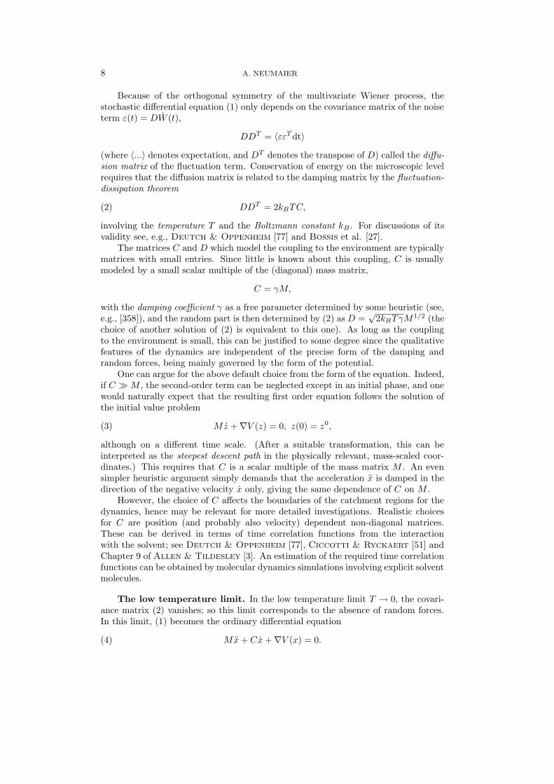
Fig. 6. A metastable state with high energy barrier
independent of the transition state energy. In particular, unless both metastablestates have nearly the same potential energy, transitions from the state with thehigher energy to that with the lower energy are much more frequent than transitionsto a higher energy level.
This implies that over sufficiently long time scales, a molecule spends most of itstime in the deepest valley near the global minimizer of the potential. It also showsthat in a collection of many (independent) molecules of the same kind, most moleculesare in a conformation close to the state with absolutely smallest potential energy. Thisis the reason why most experts (exceptions will be discussed later) expect that thegeometry defined by the global minimum of the potential energy surface is the correctgeometry describing the conformation observed in folded proteins. However, if theenergy barrier of a metastable state is sufficiently high, transition frequencies may beso low that within a biologically meaningful time the metastable state behaves likethe stable state given by the global minimum.
It should be noted that the Arrhenius law, based on classical dynamics andbistable potentials (i.e., with only two local minima), is only approximately valid.For a discussion of quantum corrections see vanGunsteren & Berendsen [334]and Voth & O’Gorman [337]. A complete review of the subject from the classicaland the quantum point of view is given by Hanggi et al. [125].
4. The harmonic approximation. In a molecular system (such as a protein)where the atoms are highly mobile, the potential energy surface has a complicatedshape; the varied topography of our earth gives an impression of what is possiblein two dimensions, and the possibilities in the high-dimensional state space are evengreater. Therefore it seems impossible to attain the ideal of studying all featuresof the dynamics; in practice one must be content with the exploration of samplepaths through the state space by means of so-called molecular dynamics calculations[26, 138, 142, 202]. These ‘solve’ the stochastic differential equation by simulatingsample paths of (1) using pseudo-random techniques. (Actually, the texts on molec-ular dynamics calculations are not clear about this relation; they usually treat thestochastic terms in an ad hoc manner that makes it difficult to assess the accuracyof the results obtained.) A detailed description of the intricacies of Monte Carlo andmolecular dynamics simulations is given in the book by Allen & Tildesley [3]; auseful survey is van Gunsteren [331]. For a discussion of numerical methods forgeneral stochastic differential equations see, e.g., Greiner et al. [121], Honerkamp

12 A. NEUMAIER
[145], Iniesta & de la Torre [151], Kloeden et al. [168], Sobczyk [300], andvan Gunsteren & Berendsen [333]. For an error analysis of numerical methodsfor stochastic differential equations see the book by Kloeden & Platen [167] andreferences there, and Bishop & Frinks [21]. The gap to the present knowledge inthe numerical analysis of deterministic differential equations (see, e.g., Hairer et al.[128, 129]) seems enormous, leaving much scope for research.
However, the high frequency behavior of the motion of molecules at low temper-ature can be studied in a simpler way by means of the so-called harmonic approxima-tion. The reason is that at high frequencies, only tiny motions are possible, and atlow temperature, the motion is confined with high probability to a neighborhood of alocal minimizer xloc. Thus it is justified to expand the potential into a Taylor seriesaround xloc, truncating it after the quadratic term. Since the gradient vanishes at alocal minimizer, we obtain the approximation
V (x) ≈ V (xloc) +1
2(x− xloc)TK(x− xloc).(7)
Here K = ∇2(xloc), the Hessian of the potential, is (in the absence of degeneracy) apositive definite symmetric matrix, called the stiffness matrix. Under our assumptionswe may also neglect damping and random forces, and obtain from (1) the lineardifferential equation for the harmonic approximation,
Mx+K(x− xloc) = 0.(8)
This differential equation has the general solution
x = xloc +∑
l
eiωltul,(9)
where the frequencies ωl and the normal modes ul (describing the vibration patternscorresponding to these frequencies) are the eigenvalues and corresponding eigenvectorsof M−1K. (Here we assumed for simplicity that no multiple eigenvalues occur.) Thefrequencies are observable as spectral lines, and (by linear response theory) the normalmodes are observable, too.
The highest frequencies occurring in proteins are of the order of 1014/sec andthe corresponding normal modes essentially correspond to stretching a C-H bond(with small compensating changes in the other bonds and the angles). Vibrationscorresponding to bond-angle bending have frequencies of the order of 1013/sec. Non-vibrational internal motions are geometrically distinguishable at time scales of around1011/sec Creighton [63]. These involve non-local changes and roughly correspondto lower frequency normal modes. While low frequencies are irrelevant for the realdynamics since the assumptions used to derive the harmonic approximation are nolonger valid, the invariant subspace spanned by all low frequency eigenvectors is thespace in which the long time dynamics takes place.
For large molecules, the eigenvalue problem is in itself already a nontrivial numer-ical task, with work growing like O(n3) for n degrees of freedom if the full spectrumis wanted. To obtain only the low frequency eigenmodes, iterative methods like theLanczos algorithm or subspace iteration can be used; see, e.g., Parlett [231]. Thework can also be reduced by various approximations. Fixing bond lengths and bondangles removes the high frequency spectrum (Levitt et al. [187], Gibrat et al.[108]). Splitting the molecule into suitable pieces allows an approximate divide-and-conquer approach by solving eigenvalue problems for the pieces and for a condensedmatrix (Hao & Harvey [131]).

MOLECULAR MODELING OF PROTEINS 13
Time scales. The frequency analysis has consequences for the molecular dynam-ics simulations. Indeed, current algorithms for tracking sample paths for solutions ofstochastic differential equations need to proceed in time steps significantly smallerthan the smallest time scale of the oscillations in order to properly trace the effect ofthe interaction between these oscillations and the random forces. Thus, time steps ofthe order of 10−15sec are called for. Since, as will be explained in the next section,the potential evaluation needed for each time step is rather expensive, only of theorder of 107 time steps can be performed in a reasonable amount of time on presentday computers, corresponding to an interval of up to a few nanoseconds.
These numbers mainly intend to give an idea of typical scales; detailed numbersdepend of course on the computer used, on the algorithms used, on the size of theprotein, on the potential employed, and on the time one is prepared to wait for theresults. In 1985, the limit was at only about 0.3 nanoseconds (Levy et al. [188]);now there are studies covering several nanoseconds (e.g., Tobias et al. [319], Guoet al [124], Soman et al. [301]) and, according to Godzik et al. [115], 100nsare feasible in a lattice approximatimation. Progress in algorithmic ingenuity andcomputer technology will push up the limit further. A recent survey of folding studiesis Caflisch & Karplus [42]; see also Daggett & Levitt [69].
On the other hand, the experimentally accessible time resolution (see, e.g., Rad-ford & Dobson [246]) is of the order of milliseconds, and typical times observedexperimentally for a protein to fold (in the absence of catalyzing enzymes) are in theorder of ∼ 10−1 − 103 seconds. This shows that we are still very far away from a com-putational treatment of the dynamics of protein folding. A critical evaluation of theresults currently obtainable with molecular dynamics simulations on some practicalproblems in drug design is given in Koppen [170]. See also McCammon & Har-vey [202], McCammon & Karplus [203]. Time saving techniques using so-calledmultiple time-steps are based on the fact that different parts of the forces change atdifferent time scales; see Teleman & Jonsson [317], Tuckerman et al. [322, 323],and Watanabe & Karplus [340].
The fastest time scales can be suppressed by fixing the fastest changing variables,especially bond lengths. (Fixing also bond angles distorts the dynamics significantly;see van Gunsteren & Berendsen2 [333].) Enforcing a vector of constraint equa-tions B(x) = 0 in a dynamical equation requires adding to the differential equation aforce term proportional to the gradient of B(x). (This can be justified by variationalprinciples.) The result is the differential-algebraic equation
Mx+ Cx+∇V (x)−∇B(x)λ = DW (t),B(x) = const.
(10)
for the pair (x, λ) consisting of the state vector and the Lagrange multiplier. In thechemical literature, people speak of constrained dynamics; see, e.g., Ryckaert etal. [258], vanGunsteren & Berendsen [332, 333] and Miyamoto & Kollman[208]. A mathematical analysis of the widely used SHAKE algorithm [258] is givenby Barth et al. [14]. For the mathematics and the solution of (non-stochastic)differential-algebraic equations in general, see the books by Brenan, Campbelland Petzold [31] and Hairer et al. [127], and the survey article Marz [193].
Some speed can also be gained by considering instead of a full molecular represen-tation of the protein a reduced representation in terms of extended atoms, where thehydrogen atoms responsible for the highest frequencies are not modeled explicitly butare treated as part of the atoms they are bonded to, thus producing extended atoms

14 A. NEUMAIER
like CH2, OH, NH, etc. and using large time steps. However, the results obtained inthis way can only be considered as rough approximations. (The models discussed inMomany et al. [212] and Troyer & Cohen [321] make even more drastic simplifica-tions to reduce the size of the problem further. See also Chan & Dill [48].) Mongeet al. [213] gains speed in a different way by assuming known secondary structure (cf.Section 7), that is frozen to limit the number of degrees of freedom.
An important development concerns the numerical methods for solving stochasticdifferential equations, that at present are mostly explicit methods. To cope with theoscillatory stiffness introduced by frequencies on multiple time scales, implicit meth-ods used successfully for the numerical solution of stiff systems of ordinary differentialequations [129], in particular so-called A-stable methods, can be adapted to take ac-count of random forces. Implicit Euler-steps were studied in Peskin & Schlick[237]. The solution of the resulting implicit equations can be achieved by local opti-mization of a dynamical energy function (Schlick [272]); see Appendix 1 for moredetails. Since the high frequencies are damped, this approach is suitable for macro-scopic models where the high frequencies are absent, or virtually uncoupled, from theslow modes. For applications to DNA supercoiling, see [275, 248].
An interesting possibility explored in Zhang & Schlick [358] is to combine theharmonic approach and the stochastic molecular dynamics approach to get a directhandle on the fast oscillations and simulate essentially the behavior on the slow modes.Zhang & Schlick [359] improve this further by solving the linearized stochasticdifferential equations exactly. Together, these developments offer a promising wayout of the limitations described above, and allow already much larger step sizes ofup to 10−12sec, valuable for sampling. Indeed, significant speedup was achieved veryrecently by a simplified version of this approach in barth et al. [15]. The resultingscheme can be considered as a method with two different timesteps: δτ = 0.5 ×10⁻¹⁵sec for solving the harmonic model, and δt = 5 × 10⁻¹⁵sec for updating theharmonic model.
Multiple time scales also arise in the dynamics of electrical circuits; multiratestrategies developed in that context (see, e.g., the papers by Denk, by Gunther &Rentrop and by Wriedt in Bank et al., [13]) may also prove useful to the dynamicsof proteins.
Robustness questions of numerical methods, related to the symplectic (Hamil-tonian) nature of the (undamped) dynamics and discussed, e.g., in Sanz-Serna [263]and Skeel et al. [292], may also turn out to be relevant. Numerical methods tayloredto Hamiltonian problems are treated in a recent book by Sanz-Serna & Calvo [264].Hamiltonian formulations are also worthy of investigation in the case of constraineddynamics. The use of symplectic integrators in molecular dynamics calculations isdiscussed in Gray et al. [119].
A good discussion of the numerical problems involved in tracing the dynamicsof molecules, together with further references, is given in the section on moleculardynamics algorithms of [218].
5. Modeling the potential. Strictly speaking, the dynamics of atoms in amolecule is governed by the quantum theory of the participating electrons. For chemi-cal applications, the so-called Born-Oppenheimer approximation is usually consideredto be adequate. In the Born-Oppenheimer approximation, one obtains the energyV (x1, . . . , xN ) at fixed nucleus positions xi as the smallest eigenvalue of an associatedpartial differential operator for the electron wave function (the Hamiltionian of theelectron system). Approximations of such eigenvalues (and of their partial derivatives

MOLECULAR MODELING OF PROTEINS 15
with respect to the nucleus positions) can be computed by so-called ab initio methods.However, for complex molecules, quantum mechanical calculations are far beyond thecomputational resources likely to be available in the near future.
Hence chemists usually use a classical description of molecules in terms of bondsand effective atomic interactions, the only trace left of the electrons being partialcharges on the atoms. Quantum theoretical calculations are restricted to the calcu-lations of properties of small constituent parts of the molecule (such as amino acids),and phenomenological models are constructed from the data obtained in this way andfrom experiment to allow extrapolation to larger molecules. Some general referenceson molecular modeling are Burkert & Allinger [37], Gund & Gund [122] andHirst [138].
The interactions of the atoms in proteins can be classified into bonded and non-bonded interactions. Bonded interactions depend on the nature of the bond: Atthe energies and time scales of interest, covalent bonds (the bonds drawn as linesin chemical formulas) are considered un-breakable, disulfide bonds (joining two closesulfur atoms, S - - - S) are slow to form and to break, and hydrogen bonds (joininghydrogen atoms with close oxygen atoms, H · · · O) are fairly easily formed and broken.
Atoms far apart are subject to non-bonded interactions: If both atoms carrypartial charges, there is the long range, slowly decaying electrostatic (Coulomb) in-teraction, and for all pairs of atoms there is the short range, fast decaying van derWaals interaction.
Hydrogen bonds and non-bonded interactions are particularly relevant for theinteraction of the molecule with the atoms of the solvent (water). The Coulombinteraction is modified by polarization effects due to the presence of solvent, and thisis modeled in the simplest case by a (often distance-dependent) dielectric constantD. However, this is somewhat inadequate, and there have been a number of recentstudies that treat the electrostatic effects due to the solvents by adding energy termsdefined by so-called continuum solvation models. Two promising methods are in use(see Cramer & Truhlar [60] for a detailed, up-to-date review): Cheaper models arebased on solvent-accessible surface area (Richmond [251], Wesson & Eisenberg[343], Schiffer et al. [270]); cf. Appendix 2. More realistic models (e.g., Gilsonet al. [113], Nicholls & Honig [223, 147]) are based on an approximate solution ofthe Poisson-Boltzmann equation
∇ · [ε(x)∇ϕ(x)]− κ(x)2 sinh(ϕ(x)) = −4πρ(x).
The solution of this nonlinear partial differential equation for the electrostatic poten-tial ϕ(x), given model assumptions defining the spatial dielectric function ε(x) (oftendiscontinuous at the molecule boundary), the Debye-Huckel parameter κ(x) (oftentaken constant), and the charge distribution ρ(x) (typically a sum of partial chargedelta functions), is a nontrivial numerical problem. (For background information ondielectrics, see, e.g., Frohlich [101]. In a constant external electric field E, thereis an additional electrostatic contribution −µ(x) · E to the potential involving themolecular dipole moment µ(x), but we do not discuss this further since usually anelectrically neutral environment is assumed.) For molecular dynamics studies of sol-vent effects, obtained by embedding the protein molecule in a large set of explicitwater molecules, see, e.g., Schreiber & Steinhauser [278, 279, 280] and Tapia[315].
The static forces in a molecule are fully determined by the formula defining thepotential V (x), so modeling the molecule simply amounts to specifying the contribu-tion of the various interactions to the potential. The models – also called force fields –
16 A. NEUMAIER
V (x) =∑
bonds
cl(b− b0)2 (b a bond length)
+∑
bond angles
ca(θ − θ0)2 (θ a bond angle)
+∑
impropertorsion angles
ci(τ − τ0)2 (τ an improper torsion angle)
+∑
dihedral angles
trig(ω) (ω a dihedral angle)
+∑
charged pairs
QiQj
Drij(rij the Euclidean distance from i to j)
+∑
unbonded pairs
cwϕ
(Ri +Rj
rij
)(Ri the radius of atom i).
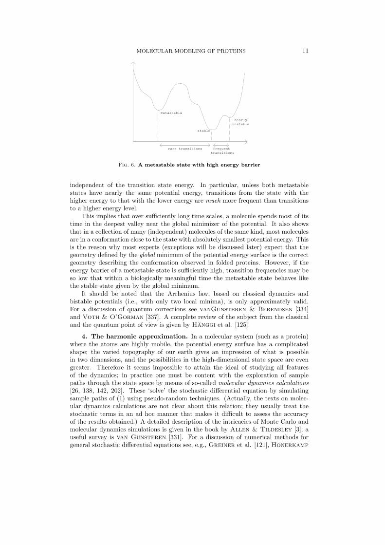
Table 1The CHARMM potential
currently in use (see [7, 33, 52, 72, 212, 219, 341, 342]; a short comparative descriptionof many force fields is given in the discussion part of Cornell et al. [58]) derive theirbasic structure from the times when molecular mechanics was only used to match theobserved structural and spectral data for rigid molecules (or molecules of very limitedmobility) to the available theory. In particular, local expansions around equilibriumdata could be used without difficulties, and this still shows in the current models.
However, local expansions are much more questionable for global optimizationand global dynamical calculations since the potential must now be approximated cor-rectly over much larger regions. We shall therefore describe in some detail one par-ticular modeling approach implemented in the molecular mechanics software packageCHARMM (Brooks et al. [33]), mention some of the numerical difficulties reportedin the use of this package, and discuss the problems associated with the use of theCHARMM potential for global purposes. The analysis leads naturally to the proposalof a revised model that avoids both the numerical difficulties and the non-physicalaspects of this model.
The CHARMM potential. The CHARMM model represents the potentialessentially as a sum of six kind of terms given in Table 1.
The Qi are partial charges assigned to the atoms in order to approximate theelectrostatic potential of the electron cloud, and D is the dielectric constant. Thequantities indexed by 0 are reference bond lengths, bond angles, and improper tor-sion angles near their equilibrium values; different constants apply depending on thenames of the atoms in the various atomic sequences, and sometimes on their loca-tion in the functional group, too. The coefficients of the trigonometric terms trig(ω),(linear combinations of cosines of multiples of ω), and the force constants c· (whose
MOLECULAR MODELING OF PROTEINS 17
magnitude reflects the strength of the respective forces) are determined, too, by thenames of the atoms corresponding to the term in question. That these constantsare indeed independent of the molecule is a basic assumption of molecular mechan-ics called transferability, an assumption not always unquestioned (Veenstra et al.[336]).
Some further terms, accounting specifically for disulfide bonds and hydrogenbonds, are also present, but will not be discussed here. (For the modeling of hy-drogen bonds see, e.g., Scheiner [267] and Ladanyi & Skaf [176].) There are alsomore complicated alternative versions for the electrostatic interaction; cf. Williams[345].
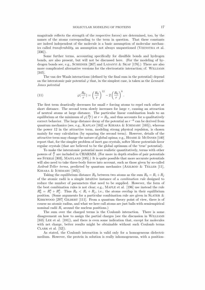
The van der Waals interactions (defined by the final sum in the potential) dependon the interatomic pair potential ϕ that, in the simplest case, is taken as the Lennard-Jones potential
ϕ(R0
r) =
(R0
r
)12
− 2
(R0
r
)6
.(11)
The first term drastically decreases for small r forcing atoms to repel each other atshort distance. The second term slowly increases for large r, causing an attractionof neutral atoms at large distance. The particular linear combination leads to anequilibrium at the minimum of ϕ(R0
r ) at r = R0, and thus accounts for a qualitativelycorrect behavior. The large distance decay of the potential as r−6 can be derived fromquantum mechanics (see, e.g., Kaplan [162] or Kihara & Ichimaru [165]), whereasthe power 12 in the attractive term, modeling strong physical repulsion, is chosenmainly for easy calculation (by squaring the second term). However, details of theattractive term may change the nature of global opima; e.g., Hoare & McInnes [140]report that, for the simpler problem of inert gas crystals, softer Morse potentials favorregular crystals (that are believed to be the global optimum of the ‘true’ potential).
To make the interatomic potential more realistic quantitatively, terms with otherpowers of R
r are included in CHARMM. (For more in depth studies of pair potentialssee Steele [303], Maitland [195].) It is quite possible that more accurate potentialswill also need to take three-body forces into account, such as those given by so-calledAxilrod-Teller terms, predicted by quantum mechanics (Axilrod & Teller [11],Kihara & Ichimaru [165]).
Taking the equilibrium distance R0 between two atoms as the sum R0 = Ri +Rjof the atomic radii is a simple intuitive instance of a combination rule designed toreduce the number of parameters that need to be supplied. However, the form ofthe best combination rules is not clear; e.g., Maple et al. [196] use instead the ruleR6
0 = R6i + R6
j . Thus R0 < Ri + Rj , i.e., the atoms overlap in their equilibriumposition. (Some arguments for a particular combination rule are given in Slater &Kirkwood [297] Gilbert [111]. From a quantum theory point of view, there is ofcourse no atomic radius, and what we here call atoms are just balls with semiempiricalnominal radii Ri around the nucleus positions.)
The sum over the charged terms is the Coulomb interaction. There is somedisagreement on how to assign the partial charges (see the discussion in Williams[345] Lee et al. [181]), and there is even some indication that, except for moleculeswith net charge, better results might be obtainable without such Coulomb termsClark et al. [52]).
As stated, the Coulomb interaction is valid only for a homogeneous dielectricmedium. However, the protein in solution is really inhomogeneous, with a position-

18 A. NEUMAIER
dependent dielectric constant that near the atoms of the protein is only about oneeighth of that of the solvent water. It is not clear how this affects the effectiveCoulomb interaction between the atoms of the proteins, and so far, only heuristiccorrections (such as a distance-dependent D) are in use. The free energy of solvationcan also be accounted for by terms proportional to the surface area exposed to thesolvent; see, e.g., Wesson & Eisenberg [343] Perrot et al. [235], Scheraga [269]and Schiffer et al. [270]. See also the molecular surface review by Conolly [56].Possibly, the solvation energy can also be accounted for by modifications of the pairpotentials and the combination rules; see Appendix 2. For the explicit modeling ofwater molecules, which is much more expensive but avoids all these problems, seeStillinger [305] and Warshel [339].
To speed up the potential evaluation, the potential is further modified by intro-ducing a cutoff distance beyond which the interatomic potential is neglected. (Recentevaluations of the effect of cut-offs on molecular dynamics simulation include Smith& Pettit [299], Steinbach & Brooks [304] and Schreiber & Steinhauser[278, 279, 280].) With such a cutoff, only a small part of the O(n2) terms in thelast sum in the potential of Table 1 need to be calculated. To make full use of theresulting sparsity (which varies from iteration to iteration), efficient data structuresmust be maintained; see, e.g., Schreiber et al. [281]. More recently, fast multipoleexpansions [25, 120, 284] and variants [70, 91] of the Ewald method (Ewald [92])were used as an alternative to cut-off methods, with a significant increase in qualityYork et al. [353, 354]. An improvement of a divide-and-conquer method by Appel[8] for fast potential evaluation is discussed in Xue et al. [352]. While useful for thesimulation of fluids, the break-even point seems to be too high to make it useful forprotein calculations.
Improving potential features. It is easy to see that the first three sums inthe potential derive their form from a truncated Taylor expansion around equilibriumvalues. Linear terms are missing since they can be incorporated into the quadraticterm by changing the value of the equilibrium constants. But cross terms like (ω −ω0)(θ−θ0), considered in Hagler [126] and to be expected in any multivariate Taylorexpansion (Bowen & Allinger [28]), are missing, too, and the main reason (to bediscovered by reading between the lines of a number of standard texts on molecularmechanics) seems to be that – in the past – the available data were not sufficient toestimate the corresponding coefficients!
However, cross terms lead to much better agreement with vibrational spectrosco-py measurements (Derreumaux & Vergoten [75], Maple et al. [196]. Moreover,cross terms can drastically modify the global behavior, especially because of the non-linearities in the non-bonded contributions, and if we ever want to obtain reliablequantitative predictions from global molecular mechanics calculations, these issuesmust be addressed much more carefully.
Since much more data are available now (and even more can be generated byab initio calculations) than at the time when the form of the potential was fixed bytradition, the old reasons for such drastic simplifications are no longer appropriate.The literature discusses some other possibilities: Adding so-called Urey-Bradley in-teraction terms (Urey & Bradley [326] and references in Chapter III of Brookset al. [34]), of the form
c‖rik − r0‖2
MOLECULAR MODELING OF PROTEINS 19
for atoms bonded as i-j-k has, locally, an effect similar to adding cross terms betweenbond lengths and bond angles. Maple et al. [196] add even some cubic interactionterms, and show that these significantly improve the fit to ab initio data. Fogarasi& Pulay [98] mention (at the end of section III) that using inverse bond lengthsinstead of bond lengths may be advantageous, and by the same reasoning one canalso argue for bond length denominators in cross terms.
For the forces accounting for the relatively easy twisting along the bonds it waswell-known that Taylor expansions were not realistic, and this accounts for the moresophisticated trigonometric terms involving the dihedral angles. However, since bondlengths, bond angles, and improper torsion angles involving the peptide bonds aremuch more rigid, the need for analogous corrections on the corresponding contribu-tions was not apparent as long as the potentials were only used for local (spectral)analysis. However, it is easy to see that globally, the terms for bond angles andimproper torsion angles are non-physical: For example, the physically equivalent an-gles θ = 160o and 200o give rise to different potentials. The minimal change neededto restore a global physically meaningful interpretation is to replace the bond anglecontributions by c(cos θ − cos θ0)2 and the improper torsion angle contributions byc(sin(τ − τ0))2, for suitable constants c. This is (approximately) realized in the forcefield used in [226, 271, 277].
Another defect of the dihedral angles (and similar remarks apply to impropertorsion angles) is the fact that these angles are geometrically undetermined when abond angle is 180o; the formulas then give the expression 0/0 for cosω and sinω. Thisinvites numerical disaster: for angles close to 180o, these quotients are numericallyvery unstable. Thus rounding errors lead to low accuracy or even essentially randomvalues for the dihedral angles, resulting in random energy contributions. Althoughequilibrium angles are typically far away from 180o, this is an important defect inglobal applications; for example it ruins (or produces unpredictable results in) anylocal optimization routine if one of the angles in an intermediate calculation (suchas a line search) happens to come close to 180o. Brooks et al. [33] observe (on p.191/2) “singularities when angles become planar (which is rather common)”; theycorrect for it in an ad hoc way by using Taylor expansions.
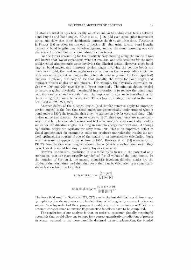
However, the natural resolution of this difficulty is to use in the potential onlyexpressions that are geometrically well-defined for all values of the bond angles. Inthe notation of Section 2, the natural quantities involving dihedral angles are theproducts sinα sinβ sinω and sinα sinβ cosω that can be calculated in a numericallystable fashion from the formulas
sinα sinβ sinω =(q × p, r)‖p‖‖q‖‖r‖ ,
sinα sinβ cosω =(p× r, r × q)‖p‖‖q‖‖r‖2 .
The force field used by Schlick [271, 277] avoids the instabilities in a different wayby replacing the denominators in the definition of all angles by constant referencevalues. As a byproduct of these proposed modifications, the evaluation of V (x) evenbecomes cheaper since no inverse trigonometric functions have to be computed.
The conclusion of our analysis is that, in order to construct globally meaningfulpotentials that would allow one to hope for a correct quantitative predictions of proteinstructure, we need to use more carefully designed terms implementing the bonded

20 A. NEUMAIER
interactions. In particular, the coefficients of such a revised model must be newlyadapted to the data available at present. For additional, experimental support of thisconclusion see Roterman et al. [256].
6. Parameter estimation. Currently, the determination of the coefficients ina potential energy model is based on data obtained by one of the following methods:
– X-ray crystallography gives the equilibrium positions of the atoms in crystallizedproteins (or rather their average over the high frequency vibrations, which introduceserrors due to anharmonic effects). A basic text is Giacovazzo [106]; specifically forproteins see, e.g., Zanotti [357], Fortier et al. [99].
– Nuclear magnetic resonance (NMR) spectroscopy, (see, e.g., Jardetzky &Lane [157], Torda & van Gunsteren [320]), gives position data of proteins insolution.
– Ab initio quantum mechanical calculations [80, 98, 196, 211, 236] give ener-gies, energy gradients, and even energy Hessians (i.e., second derivative matrices) atarbitrarily selected positions of the atoms, for molecules in the gas phase;
– Measurements of energy spectra give rather precise eigenvalues of the Hessian;– Thermodynamical analysis gives specific heats, heats of formation, conforma-
tional stability information, related to the potential in a more indirect way, via sta-tistical mechanics.
The model parameters are adapted to data from one or several of these sources byusing a mixture of least squares fitting and more heuristic or interactive procedures.Starting values for the coefficients come from general knowledge about atomic radii,average bond lengths and angles, and (for the force constants) from the frequenciesof the oscillations of these quantities. The resulting rough parameters are then fittedto the data using a least squares approach.
The state of the art of numerical methods for least squares calculations is surveyedin Bjorck [22, 23] for the linear case. In addition, recent work by Matstoms [201]on multifrontal orthogonal factorizations for large and sparse least squares problemsis relevant. The nonlinear case is reduced to the linear case, most commonly by meansof damped Gauss-Newton steps, see, e.g., Dennis & Schnabel [74], Fletcher [97].
For a survey of parameter fitting procedures used in molecular mechanics seeHopfinger & Pearlstein [148]. More heuristic techniques are used to correctthe parameters to match spectral data available, e.g., for the amino acids; see, e.g.,[33, 175]. A detailed description of the development of a potential model is givenby Lifson [190]. From a mathematical point of view, the ab initio approach (withsecond derivative information) poses interesting questions about multidimensionalHermite interpolation (or approximation) and the optimal choice of trial points forthe quantum mechanical calculations; since the least squares problems are here linear,traditional methods for the optimal design of experiments (see, e.g., Atkinson [9],Atwood [10], Pukelsheim [241] and the books by Fedorov [94] or Silvey [286])should lead to improved fits for the same amount of work.
The assessment of the sensitivity of the parameters with respect to the input datagenerally received very little attention. Maple et al. [196] mention the calculation ofparameter uncertainties, but give no details on their magnitude. One reason for theimportance of parameter uncertainties is that parameters with large uncertainties areunlikely to be transferable. Thacher et al. [318] discuss other applications of thesesensitivities.
The sensitivity of equilibrium internal coordinates with respect to changes in thevalues of the parameters is discussed in Susnov [314].

MOLECULAR MODELING OF PROTEINS 21
Knowledge of such sensitivity information gives information on the quality of themodel potential, and helps to assess the relative importance of the various terms inthe potential; cf. Rabitz [243]. Together with the parameter uncertainties it alsogives an idea of the accuracy obtainable in potential minimizations, and hence of theaccuracy to which these minimizations are worth computing.
In principle, sensitivity information can be obtained together with the leastsquares calculation (see, e.g., Draper & Smith [83]); but the improvements gainedthrough the spectral information can be similarly assessed only when this informationis combined with the position data available in a larger (and more nonlinear) leastsquares problem.
Ab initio potentials. Problems of a different kind appear in attempts to derivethe potential from basic principles. Strictly speaking, the quantum mechanical abinitio potential is not the right potential to use in molecular mechanics applicationssince it gives as potential energy the quantity referred to by chemists as the enthalpyH. But the potential relevant for calculations at fixed finite temperature T > 0,the Gibbs free energy G = H − TS, has a correction term involving the conforma-tional entropy S of the system. The conformational entropy is proportional to thelogarithm of the number of microscopically distinguishable configurations belongingto an observed macrostate and is thus roughly proportional to the logarithm of thevolume of the catchment region of a metastable state. Thus large flat minima (havinga large catchment region) or large regions covered by many shallow local minima (cor-responding to a glassy regime) are energetically more favorable than a narrow globalminimum if this has only a slightly smaller potential.
Some early calculations are reported by Farnell et al. [93]. To estimate theconformational entropy, Creighton [62], p. 161, apparently only counts local min-imizers, taking his intuition from simple random polymers where these minima canbe assumed to be equidistributed with similar-sized catchment regions. For the muchmore complex energy surfaces of proteins, this assumption seems questionable. Go& Scheraga [118] (see also Scheraga [268], who surveys alternative approachesto entropy, too) use second derivative information on all nearly global minima (atx(1), x(2), . . .) to approximate the conformational entropy of a minimum at x(m) by
Sm = −kB log pm + kB log∑
k
pk,(12)
where
pm =exp(−V (x(m))
kBT)
√det∇2V (x(m))
.(13)
(The log∑
term can be ignored since it shifts the entropy and hence the free energyby the same term for all minima.) This formula derives from statistical mechanicsby replacing the potential near each nearly global minimum by its quadratic Taylorexpansion. Anharmonicities (i.e., effects due to non-quadratic higher order terms)are thus not taken into account. Molecular dynamics simulations, started at a nearlyglobal minimizer and exploring the neighborhood over a sufficiently long time interval,would in principle allow the determination also of anharmonic contributions to theconformational entropy. (Formula (12) makes only sense at the local minima them-selves. For non-equilibrium configurations, one has to work with partition functions,that are more difficult to handle; cf. again [118].)

22 A. NEUMAIER
Currently, entropy considerations are often addressed computationally in a qual-itative fashion only, using very simple (e.g., lattice) models together with techniquesfrom statistical mechanics. A survey of typical results obtainable in that way, andmany further references on the statistical mechanics approach, are given in Wolynes[347].
Entropy of mixing with the solvent is another term that may play a role; seeChen et al. [49]. See also Abagyan [1] for a discussion of the various terms thatneed to be added to the ab initio potential to get a more realistic potential.
For semiempirical potentials fitted to experimental data, these fine points appearsomewhat less important in view of the other approximations made: the resultingpotentials are always effective potentials adapted to the form of potential used andthe experimental conditions from which the data are derived. However, this impliesthat caution is needed when combining data from different sources.
7. The native state. We concluded Section 3 with the remark that most ex-perts expect that the geometry defined by the global minimum of the potential energysurface is the correct geometry describing the conformation observed in folded pro-teins. In the present section we look at the structure of the potential landscape. Wealso take a critical look at the statement that the folded state is given by the globalminimum, and discuss some alternatives considered in the literature.
The most challenging feature of the protein folding problem is the fact that theobjective function has a huge number of local minima, so that a local optimization islikely to get stuck in an arbitrary one of them, possibly far away from the desired globalminimum. People working in the field expect an exponential number of local minima.Estimates I have seen range from 1.4n to 10n for a protein with n residues; the highestestimate is from Creighton [62], p. 161. For very general energy minimizationproblems, combinatorial difficulty (NP-hardness) can be proved by showing that thetraveling salesman problem can be phrased as a minimization of the sum of two-bodyinteraction energies (Wille & Vennik [344]), but the potential is very contrived,and the result implies nothing for more realistic situations.
For less structured problems with more symmetries, like the problem of the opti-mal configuration for a cluster of n identical atoms with a Lennard-Jones interaction(11), the number of local minima appears to grow even more violently; an estimate
by Hoare [139] is O(1.03n2
). However, most of these local minima would have alarge potential energy and thus be irrelevant for global optimization; the number oflow-lying minima is more likely to grow simply exponential in n, too. A remarkableobservation of Hoare & McInnes [140] reveals that using in place of the Lennard-Jones pair interactions more realistic Morse functons gives cluster potentials with amuch smaller number of local minima. Thus it may be that, also in the protein foldingcase, more realistic potentials will be easier to handle than current simpler models.
A bead model. To get a feeling for the origin of the exponential number oflocal minima, consider the following intuitive bead model, that ignores all non-localinteraction and simulates the local interaction by a rubber band. Imagine a chainof n irregularly shaped beads (20 different kinds, corresponding to the amino acids)threaded along a rubber band knotted at one end and held at the other end. Therubber band tries to contract, and the beads arrange themselves in a way as tominimize the potential energy (tension). Now consider fixing the top i beads ofthe chain while rotating the (i + 1)st bead along the chain together with the restof the chain below. Because of the irregular shape of the beads, the rotated bead
MOLECULAR MODELING OF PROTEINS 23
and the bead above it move somewhat apart to allow the rotation, but after somelocal irregularity is overcome the beads can come closer together again. Thus theenergy increases at first, passes a saddle point (a local maximum along the reactioncoordinate), and moves towards a new local minimum. Depending on the shapeof the two adjacent beads, there may be a different number mi of locally optimalarrangements of the two beads. Noticing that rotations at different beads can beperformed independently, we see that the total number of different local optima ism1 · . . . ·mn−1, and if each mi is greater than one, this gives an exponential numberof possibilities.
Of course, this model is very simplistic; interaction in a realistic molecule ismuch more complex and also non-local. But the model allows one to understandthe qualitative origin of the large diversity of local minima possible and is likely tobe realistic in this respect. So-called genetic algorithms for global optimization (seebelow) attempt to make use of the insight from such simple analogies by allowingmutations and crossing over between candidates for good local optima in the hope toderive even better ones.
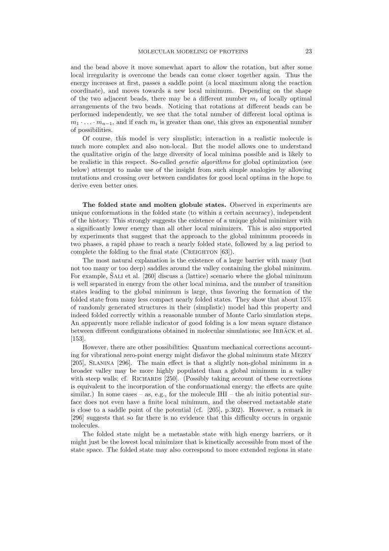
The folded state and molten globule states. Observed in experiments areunique conformations in the folded state (to within a certain accuracy), independentof the history. This strongly suggests the existence of a unique global minimizer witha significantly lower energy than all other local minimizers. This is also supportedby experiments that suggest that the approach to the global minimum proceeds intwo phases, a rapid phase to reach a nearly folded state, followed by a lag period tocomplete the folding to the final state (Creighton [63]).
The most natural explanation is the existence of a large barrier with many (butnot too many or too deep) saddles around the valley containing the global minimum.For example, Sali et al. [260] discuss a (lattice) scenario where the global minimumis well separated in energy from the other local minima, and the number of transitionstates leading to the global minimum is large, thus favoring the formation of thefolded state from many less compact nearly folded states. They show that about 15%of randomly generated structures in their (simplistic) model had this property andindeed folded correctly within a reasonable number of Monte Carlo simulation steps.An apparently more reliable indicator of good folding is a low mean square distancebetween different configurations obtained in molecular simulations; see Irback et al.[153].
However, there are other possibilities: Quantum mechanical corrections account-ing for vibrational zero-point energy might disfavor the global minimum state Mezey[205], Slanina [296]. The main effect is that a slightly non-global minimum in abroader valley may be more highly populated than a global minimum in a valleywith steep walls; cf. Richards [250]. (Possibly taking account of these correctionsis equivalent to the incorporation of the conformational energy; the effects are quitesimilar.) In some cases – as, e.g., for the molecule IHI – the ab initio potential sur-face does not even have a finite local minimum, and the observed metastable stateis close to a saddle point of the potential (cf. [205], p.302). However, a remark in[296] suggests that so far there is no evidence that this difficulty occurs in organicmolecules.
The folded state might be a metastable state with high energy barriers, or itmight just be the lowest local minimizer that is kinetically accessible from most of thestate space. The folded state may also correspond to more extended regions in state

24 A. NEUMAIER
space where there are many close local minima of approximately the same energy asat the global minimum.
This last situation corresponds to what physicists refer to as glassy behavior(see the statistical dynamics treatment surveyed in Wolynes [347] and referencesthere), and there are some indications from molecular dynamics simulations (Elber& Karplus [89], Honeycutt & Thirumalai [146]) that this might be the situationin typical energy surfaces of proteins. (Temperature effects also play a role, seeAbkevich et al. [2].) On the other hand, calculations of Iori et al. [152], usinga different model, arrive at the opposite conclusion.
Camacho & Thirumalai [43] find that, in lattice models, there appear to beexponentially many local minimum structures and exponentially many compact struc-tures, but the number of compact local minimum structures seens to be nearly inde-pendent of the number of residues.
More recent studies (Karplus et al. [163], Leopold et al. [185] Onuchic et al.[227], Sali et al. [260, 261, 262], Wolynes et al. [348]; see also Hao & Scheraga[132] and a very informative survey by Dill et al. [78]) seem to reach an agreementin that the native state is a pronounced global minimizer that is reached dynamicallythrough a large number of transition states by an essentially random search through ahuge set of secondary, low energy minima (representing a glassy molten globule state),separated from the global minimum by a large energy gap. In simulations with crudelattice models (see, e.g., Dill et al. [78], pp. 594-595 for the merits and faults ofthis simplifying assumption), this scenario appears to be the necessary and sufficientconditions for folding in a reasonable time. (Crude off-lattice models also appear toconfirm this statement; see Irback et al. [153, 154].)
It explains the so-called Levinthal paradox (Levinthal [186]) that the time aprotein needs to fold is by far not large enough to explore even a tiny fraction of alllocal minima only. However, fast collapse to a compact molten globule state, followedby a random search through the much smaller number of low energy minima couldaccount for the observed time scales, and the energy gap provides the stability ofthe native state over the molten globule state. The time-limiting step is provided bythe task to drive the molten globule into one of the transition states to the nativegeometry. Experimental characterizations of molten globule states are discussed inDobson [81] and Miranker & Dobson [207].
On the other hand, the studies mentioned disagree on many of the details, andthe simplified drawings of the qualitative form of the potential energy surface aremutually incompatible between different schools.
This shows that the interpretation of the literature on this point is difficult. Atthe present stage of development, unless the models are extremely simple, numericalcalculations do not allow one to check reliably whether a global minimizer has beenfound; all that can be said is that the minimizers found were the best ones in anincomplete search. Discrepancies with experiments or with theoretical expectationsmight as well be interpreted as artifacts created by deficiencies of the potential used;the model accuracy is probably not higher than the distance between several near-global minima. And the papers with the more impressive simulations do not evenclaim that their (lattice) models represent more than only rough qualitative aspectsof real proteins.
A serious limitation of many simulation studies is the fact that the presence of asolvent is poorly accounted for in the models used for folding simulations. Methodsbased on the Poisson-Boltzmann equation or the solvent-accessible surface are too
MOLECULAR MODELING OF PROTEINS 25
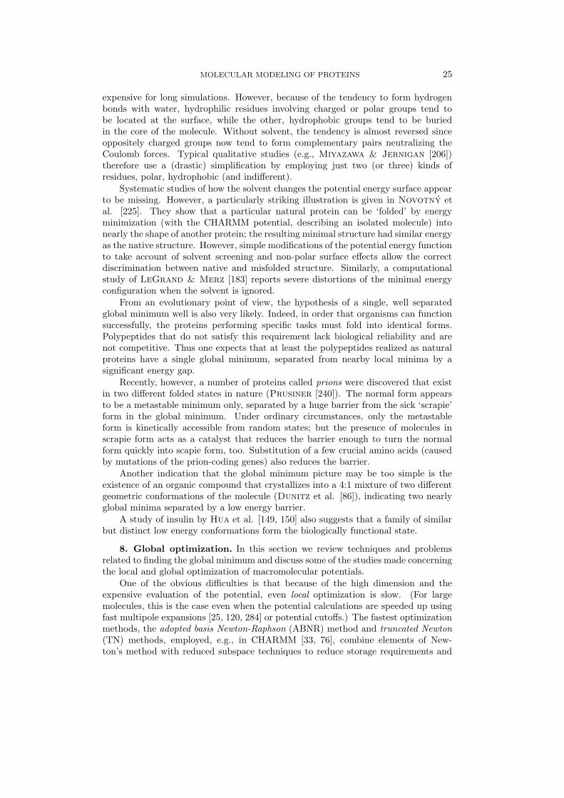
expensive for long simulations. However, because of the tendency to form hydrogenbonds with water, hydrophilic residues involving charged or polar groups tend tobe located at the surface, while the other, hydrophobic groups tend to be buriedin the core of the molecule. Without solvent, the tendency is almost reversed sinceoppositely charged groups now tend to form complementary pairs neutralizing theCoulomb forces. Typical qualitative studies (e.g., Miyazawa & Jernigan [206])therefore use a (drastic) simplification by employing just two (or three) kinds ofresidues, polar, hydrophobic (and indifferent).
Systematic studies of how the solvent changes the potential energy surface appearto be missing. However, a particularly striking illustration is given in Novotny etal. [225]. They show that a particular natural protein can be ‘folded’ by energyminimization (with the CHARMM potential, describing an isolated molecule) intonearly the shape of another protein; the resulting minimal structure had similar energyas the native structure. However, simple modifications of the potential energy functionto take account of solvent screening and non-polar surface effects allow the correctdiscrimination between native and misfolded structure. Similarly, a computationalstudy of LeGrand & Merz [183] reports severe distortions of the minimal energyconfiguration when the solvent is ignored.
From an evolutionary point of view, the hypothesis of a single, well separatedglobal minimum well is also very likely. Indeed, in order that organisms can functionsuccessfully, the proteins performing specific tasks must fold into identical forms.Polypeptides that do not satisfy this requirement lack biological reliability and arenot competitive. Thus one expects that at least the polypeptides realized as naturalproteins have a single global minimum, separated from nearby local minima by asignificant energy gap.
Recently, however, a number of proteins called prions were discovered that existin two different folded states in nature (Prusiner [240]). The normal form appearsto be a metastable minimum only, separated by a huge barrier from the sick ‘scrapie’form in the global minimum. Under ordinary circumstances, only the metastableform is kinetically accessible from random states; but the presence of molecules inscrapie form acts as a catalyst that reduces the barrier enough to turn the normalform quickly into scapie form, too. Substitution of a few crucial amino acids (causedby mutations of the prion-coding genes) also reduces the barrier.
Another indication that the global minimum picture may be too simple is theexistence of an organic compound that crystallizes into a 4:1 mixture of two differentgeometric conformations of the molecule (Dunitz et al. [86]), indicating two nearlyglobal minima separated by a low energy barrier.
A study of insulin by Hua et al. [149, 150] also suggests that a family of similarbut distinct low energy conformations form the biologically functional state.
8. Global optimization. In this section we review techniques and problemsrelated to finding the global minimum and discuss some of the studies made concerningthe local and global optimization of macromolecular potentials.
One of the obvious difficulties is that because of the high dimension and theexpensive evaluation of the potential, even local optimization is slow. (For largemolecules, this is the case even when the potential calculations are speeded up usingfast multipole expansions [25, 120, 284] or potential cutoffs.) The fastest optimizationmethods, the adopted basis Newton-Raphson (ABNR) method and truncated Newton(TN) methods, employed, e.g., in CHARMM [33, 76], combine elements of New-ton’s method with reduced subspace techniques to reduce storage requirements and
26 A. NEUMAIER
to limit the amount of work done at each iteration. A comparison of these methodsdeveloped by chemists with some of the recent methods for large scale optimizationdeveloped by the optimization community, in particular truncated Newton methods(Nash [217], Schlick & Overton [276], Schlick & Fogelson [274]), is given ina recent survey article by Schlick [273]. For an adaptation of the truncated Newtonoptimization package TNPACK [274] to the molecular mechanics package CHARMM[33] see Derreumaux et al. [76].
However, since the objective function has a huge number of local minima, a lo-cal optimization is likely to get stuck before the global minimum is reached. Thussome kind of global search is needed to find the global minimum with some reli-ability. Leach [180], Scheraga [268], and Pardalos et al. [229] survey, fromdifferent perspectives, the different methods for global optimization that have beenused so far on molecular conformation problems. Together with the proceedingsof the workshop on global minimization of nonconvex energy functions by Par-dalos et al. [230], these give an up to date bibliography on this part of the lit-erature. Online information on global optimization in general (including public do-main software packages) can be found on the World Wide Web, e.g., at the addresshttp://solon.cma.univie.ac.at/∼neum/glopt.html.
Instead of describing technical details of the various methods (these vary fromauthor to author, and can be found in the citations above), I want to present a vividinformal view of the most useful basic techniques, their strengths and weaknesses.The methods that are considered by the folding community most useful at presentare simulated annealing, genetic algorithms, and smoothing methods. All three arebased on analogies to natural processes where more or less global optima are reached.
Simulated annealing. Introduced by Kirkpatrick [166], simulated annealingtakes its intuition from the fact that the heating (annealing) and slowly cooling ametal brings it into a more uniformly crystalline state, that is believed to be the statewhere the free energy of bulk matter takes its global minimum. (Incidentally, evenfor the simplest potentials, it is still an unsolved problem whether this is indeed truewith mathematical rigor. For some results in this direction, see Radin & Schulmann[247]). The role of temperature is to allow the configurations to reach higher energystates with a probability given by Boltzmann’s exponential law, so that they canovercome energy barriers that would otherwise force them into local minima. Thisis quite unlike line search methods and trust region methods on which good localoptimization programs are based (see, e.g., Gill et al. [112]).
In its original form, the simulated annealing method is provably convergent (ina probabilistic sense) but exceedingly slow; various ad hoc enhancements make itmuch faster. In particular, except for simple problems, success depends very much onthe implementation used. For results of simulated annealing techniques for proteinstructure prediction see, e.g., Kawai [164], Shin & Jhon [285].
Genetic algorithms. Introduced by Holland [143], genetic algorithms makeuse of analogies to biological evolution by allowing mutations and crossing over be-tween candidates for good local optima in the hope to derive even better ones. Ateach stage, a whole population of configurations are stored. Mutations have a similareffect as random steps in simulated annealing, and the equivalent of lowering of thetemperature is a rule for more stringent selection of surviving or mating individuals.
The ability to leave regions of attraction to local minimizers is, however, drasti-cally enhanced by crossing over. This is an advantage if, with high probability, the

MOLECULAR MODELING OF PROTEINS 27
crossing rules produce offspring of similar or even better fitness (objective functionvalue); if not, it is a severe disatvantage. Therefore the efficiency of a genetic algo-rithm (compared with simulated annealing type methods) depends in a crucial wayon the proper selection of crossing rules. The effect of interchanging coordinates isbeneficial mainly when these coordinates have a nearly independent influence on thefitness, whereas if their influence is highly correlated (such as for functions with deepand narrow valleys not parallel to the coordinate axes), genetic algorithms have muchmore difficulties. Thus, unlike simulated annealing, successful tuning of genetic al-gorithms requires a considerable amount of insight into the nature of the problem athand. For a more detailed discussion of genetic algorithms in general see Davis [73];for applications to protein folding see, e.g., Brodmeier & Pretsch [32], Kawai[164], Le Grand & Merz [183], ShinJhon [285].
Both simulated annealing methods and genetic algorithms are, in their simplerforms, easy to understand and easy to implement, features that invite potential usersof optimization methods to experiment with their own versions. The methods oftenwork, if only slowly, and lacking better alternatives, they are very useful tools forbiochemists, where the primary interest is to find (near-)solutions now, even whenthe reliability is uncertain.
To make simulated annealing methods and genetic algorithms efficient, clever en-hancements are essential. However, theoretical work on explaining the effectiveness ofuseful enhancements is completely lacking. I also haven’t seen careful comparisons ofthe various options available and their comparative evaluation on standard collectionsof test problems.
Smoothing methods. First suggested by Stillinger [306] and Stillinger &Weber [308], smoothing methods are based on the intuition that, in nature, macro-scopic features are usually an average effect of microscopic details; averaging smoothesout the details in such a way as to reveal the global picture. A huge valley seen fromfar away has a well-defined and simple shape; only by looking more closely, the manylocal minima are visible, more and more at smaller and smaller scales. The hope isthat by smoothing rugged potential energy surface, most or all local minima disap-pear, and the remaining major features of the surface only show a single minimizer.By adding more and more details, the approximations made by the smoothing areundone, and finally one ends up at the global minimizer of the original surface.
While it is quite possible for such a method to miss the global minimum (so thatfull reliability cannot be guaranteed, and is not achieved in the tests reported by theirauthors), a proper implementation of this idea at least gives very good local minimawith a fraction of the function evaluations needed for the blind annealing and geneticmethods. It should be possible to further increase the reliability of the methodsby using a limited amount of global search in each optimization stage, though thisappears not to have been done so far.
A conceptually attractive smoothing technique is the diffusion equation method(Piela et al., [239], Li & Scheraga [189]), where the original potential function V (x)is smeared out by artificial diffusion. The solution V (x, t) of the diffusion equation
Vxx(x, t) = Vt(x, t)
with initial condition V (x, 0) = V (x), that can be solved explicitly if V (x) is a linearcombination of Gaussians in ‖xi − xk‖, gets smoother and smoother as t gets larger;for large enough t, it is even unimodal. Thus V (x, t) can be minimized by local

28 A. NEUMAIER
methods when t is sufficiently large, and using the minimizer at a given t as a startingpoint for a local optimization at a smaller t, a sequence of local minimizers of V (x, t)for successively smaller t is obtained until finally, with t = 0, a minimizer of theoriginal potential is reached. Unfortunately, for general functions, smoothing is veryexpensive, and at present the methods are practically useful mainly when the potentialis a sum of univariate functions of distances between atomic coordinates. With minorerrors, the potentials currently used in protein modeling can be approximated in thisway.
Positive and negative results for both Lennard-Jones clusters and oligopeptidesare reported in Kostrowicki et al. [172, 173]. Modifications to take account of therigid structure of bond lengths and bond angles are discussed in Kostrowicki &Scheraga [174]. Similar techniques for smoothing have been proposed and appliedto potential energy surfaces by Coleman et al. [55], Moree & Wu [214, 215],Shalloway [283] and Wu [349].
A different smoothing technique is proposed in Dill et al. [79]. They constructa surrogate potential surface by fitting an underestimating function to known localoptima, hoping that the global optimum lies near the minimizer of this surrogatefunction. A kind of hybrid method between simulated annealing and smoothing isthe quantum mechanical annealing technique of Straub et al. [4, 192, 310].
While the above techniques are motivated by nature it is important to rememberthat processes in nature need not be the most efficient ones; at best it can be as-sumed to be efficient given the conditions under which they have to operate. (Much ofour present technology has vastly surpassed natural efficiency, by unnatural means.)Even assuming that nature solves truly global optimization problems (a disputableassumption), simple lower estimates for the number of elementary steps – roughlycorresponding to function evaluations – available to natural processes to converge are(in chemistry and in biology) in the range of 1015 or even more. Thus to be successfulon the computers of today or the near future, we must find methods that are muchfaster, exploring the configuration space in a planned, intelligent way, not with a blindcombination of chance and necessity. And the challenge is to devise methods that canbe analyzed sufficiently well to guarantee reliablility and success.
Some other recent papers don’t fit one of the above general paradigmas. Byrd etal. [39, 40, 41] and van der Hoek [329] employ a mixed stochastic sampling, localoptimization and global subset optimization strategy specially adapted to parallelcomputing. Vajda & Delisi [327] use dynamic programming. Billeter [20] workswith an ellipsoid algorithm.
Branch and bound methods. Traditionally, see, e.g., Nemhauser & Wolsey[220], branch and bound methods are the method of choice for solving global opti-mization problems of a combinatorial nature, formulated as mixed integer programs.Since protein folding problems have a combinatorial aspect, branch and bound meth-ods appear to be suitable for this task as well. However, since the coordinates arecontinuous variables instead of discrete ones, the methods do not immediately extendto potential minimization.
Though at present limited to small oligopeptides, the branch and bound meth-ods developed by Maranas & Floudas [197, 198, 199, 200] are potentially mostinteresting since they lead to lower bounds on the minimal energy. They are the onlycurrent methods that allow an assessment of the quality of the local minima obtained,and combined with the sufficient conditions for global minima derived in Neumaier

MOLECULAR MODELING OF PROTEINS 29
[222], they may allow one to actually prove global optimality of the best local opti-mizers obtained, and thus may remove the aura of ambiguity inherent in all ‘global’calculations of the past.
In the worst case, branch and bound methods take an exponential amount ofwork; but while this might well be realistic for the case of Lennard-Jones clusters,there are signs that the situation is much better than worst case with potentialsfor proteins. Indeed, a recent study by Buturovic et al. [38] abstracted from thecontinuous global optimization problem a cruder combinatorial version based on areduction of the Ramachandran plots (explained in the next section) to a discreteset of points, and showed that an exhaustive search for the solution of the resultingcombinatorial optimization problem was feasible for several small proteins. With morerefined techniques for the construction of underestimating functions, there is hope forrepeating the calculations without the need for such drastic simplifications. Manyof the heuristic techniques used currently for searching the conformational space ofmolecules (see Leach [180] and Saunders et al. [265]) can be adapted to or combinedwith the branch and bound approach to take advantage of the structural insights ofcurrent chemistry.
Branch and bound methods will ultimately allow one not only to calculate theglobal minimum reliably, but also to find all local minima and saddle points withina certain energy margin of the global minimum. This is essentially the problem offinding all zeros of the nonlinear system ∇V (x) = 0 that satisfy a constraint on thesignature of the Hessian and on the value of V . Such problems can already be han-dled in low dimensions by branch and bound methods, combined with techniques forinterval analysis (Hansen [130], Neumaier [221]), and it should be possible to com-bine these techniques with the underestimation techniques of Maranas & Floudas[197, 198, 199]. Some results of a branch and bound method on oligopeptides aregiven in Androulakis et al. [5].
Since this would provide information about the low-lying transition states andmetastable states, developing these branch and bound methods to work for higher-dimensional problems will allow one to study not only the folded equilibrium statebut also the final stages of folding and the early stages of unfolding. (However,Eksterowicz & Houk [88] observed that semiempirical potentials derived fromstable molecules may be not accurate enough for the calculation of transition states.See also Anet [6].)
Since no near global minimum will be missed, calculation of the entropy contri-butions (12), (13) will allow finding the global minimum of the Gibbs free energy,that is more likely to match the true folded state. See Saunders et al. [265] for aperformance study of several methods for finding most (or perhaps even all) low-lyinglocal minima of a cycloheptadecane potential. (A huge number of near global min-ima – and a fortiori transition states, as expected for proteins if they exhibit glassybehavior, would, however, result in exponentially large space and time requirements.)
Constraints. In view of the expected huge number of local minima, techniquesthat reduce the size of the region in state space that must be searched for the globalminimum are very valuable (Head-Gordon et al. [134, 135, 133], van der Graaf& Baas [328]). Trivial restrictions that can be used are two-sided bounds on bondlengths and bond angles, and lower bounds on contact distances of arbitrary pairs.The bounds can be implemented either as hard bounds (via constraints) or as softbounds (via penalty terms). A book by Mockus [209] discusses stochastic methodsfor constrained global optimization.

30 A. NEUMAIER
More generally, bounds on distances would allow one to combine the optimizationapproach to molecular modeling and the distance geometry approach surveyed inCrippen [65], Crippen & Havel [66] and Blaney & Dixon [24]. Steps in thisdirection are discussed in Crippen [64] and Scarsdale et al. [266]; they assumethat further distance information is known about the molecule, e.g., from nuclearmagnetic resonance (NMR) spectroscopy.
In the absence of such detailed experimental information, the most likely candi-dates for a further significant reduction are constraints for the dihedral angles alongthe backbone. Indeed, biochemists have known for a long time experimentally thatthese dihedral angles are severely constrained. They discuss the pertaining informa-tion under the concept of secondary structure treated in the next section.
A little simpler is the constrained optimization problem known as side chainprediction. The task is to find the positions of the side chains of a protein, given thepositions of the backbone atoms. See, e.g., Lee & Subbiah [182], Tuffery et al.[324], Dunback & Karplus [84, 85].
The refinement of crystallographic data of limited (known) accuracy by meansof a model potential, cf. Brunger et al. [36], can also be treated as a globalconstrained optimization problem, and since the given data already strongly restrictthe conformation space, this problem may even be solvable in high dimensions. Thesame holds for the construction of Cartesian coordinates from distance data obtainedby nuclear magnetic resonance (NMR) spectroscopy (Scarsdale et al. [266], Torda& van Gunsteren [320]) by finding the global minimum of a weighted sum
Vdc =∑
i,ki6=k
cik(‖xi − xk‖−3 − r−3ik )2
to find the Cartesian coordinates that best match a set of measured distances rik.The related problem of finding the optimal superposition of two geometries for
a molecule is discussed in Kabsch [160]. This technique is important since it allowsthe comparison of experimental coordinates of a molecule with those derived fromcomputational predictions.
9. Simplified models. Various simplifications of the protein folding problemare studied in the literature in order to understand the global optimization processand to simplify the development and testing of optimization algorithms. The Lennard-Jones cluster problem (a problem also of independent interest in applications) hasextra symmetry. Hence more specialized techniques can be used (see, e.g., [224, 139,57, 351]) that allow one to reach rather low lying minimizers even for a huge numberof atoms ([350] reports calculations for up to 105 atoms). If one adds constraintsfor fixed bond lengths one gets the models discussed in Pardalos et al. [229]. Evensimpler are the ‘toy models’ of Stillinger et al. [307], the bead models of Fergusonet al. [95], and the lattice models considered by Phillips & Rosen [238]. A surveyof simplified models is given by Troyer & Cohen [321].
Some of the simplified models are accurate enough so that the resulting optimalstructures resemble the real native structures, and still simple enough so that theglobal optimization by one of the methods discussed above appears feasible. Togetherwith a final refinement of the structure by a local optimization, this is believed to givealready useful structural information, though structural mistakes cannot be excluded.
These models fall into several classes:

MOLECULAR MODELING OF PROTEINS 31
Full energy models. Simplified full energy models have fixed bond lengths,bond angles and some torsion angles (e.g., around the peptide bond). At this level ofapproximation, many of the difficulties explained in the section on potentials becomeirrelevant. The only degrees of freedom are an independent set of torsion angles, whichlimits the number of variables to ∼ 3n− 5n, where n is the number of residues. Suchmodels are regarded as highly reliable; but function evaluation is expensive due to therequired transformations between angles and Cartesian coordinates. The reconstruc-tion of met-enkephalin (5 residuess, 19 torsion angles) is reported in Kostrowicki &Scheraga [173], using the diffusion equation method; in the latter case, a near-globalminimum structurally similar to the native geometry is found.
Statistical backbone potential models. Here only the backbone (or the back-bone and a side chain center, or even only the set of Cα atoms) is modeled, with fixedbond lengths, bond angles and peptide bond torsion angles (or fixed distant of neigh-boring Cα’s, respectively). In both cases, the number of variables is reduced to 2n,and the potential has a simple form, determined by assuming that a set of knownstructures is an equilibrium ensemble of structures, so that the energy can be cal-culated from Boltzmann’s law and statistics on the known structures. In order toobtain a useful statistics, the protein structures used must be carefully selected; see,e.g., Hobohm et al. [141]. A more detailed overview can be found in Sippl [287].Other statistical force field construction techniques are discussed in Bauer & Beyer[17] and Ulrich et al. [325]. The fact that the potential is now directly derived fromgeometric data implies that it automatically takes account of solvation and entropycorrections; on the other hand, one only gets a mean potential of less resolution. Re-constructions using such mean potentials are reported by Sun [313] for mellitin (26residues), APPI (36 residues) and crambin (46 residues) using simulated annealing, bySun [312] for mellitin and apamin (18 residues) using genetic algorithms, by Gunn etal. [123] for myoglobin (153 residues) using a combination of simulated annealing andgenetic algorithms, and by Sippl et al. [289] for lysozyme, myoglobin and thymosin.In all these papers, results are only ‘native-like’ when compared with the experimentalstructures.
Related techniques based on backbone models with terms involving informationfrom Ramachandran plots (see next section) are discussed in Dill et al. [79]. As inearlier models (e.g., Honeycutt & Thirumalai [146]), the amino acids are treatedin a reduced descriprion only, based on their hydrophilic or hydrophobic affinity.
Lattice models with contact potentials. Here the molecule is forced to haveits atoms lying on lattice positions, and the potential is a sum of contact energiestaken from tables derived again from statistics on databases. Now function evalua-tion is extremely cheap (addition of table entries for close neighbors only, resultingin a speedup factor of two order of magnitudes), and the problem has become oneof combinatiorial optimization. The quality of a lattice model is mainly determinedby its coordination number, the number of permitted sites for a Cα atom in a residueadjacent to a residue with a Cα atom in a fixed position. Models used to studyqualitative questions of statistical mechanics (e.g., Sali et al. Sali2) usually use anearest neighbor cubic lattice (with coordination number 6). While these are occa-sionally used for structure prediction (e.g., Rabow & Scheraga [244], who alsoreport inadequacies of the Miyazawa-Jernigan-Cowell [59] contact potential), a goodrepresentation of Cα−Cα distances and angles requires at least a face-centered cubic(FCC) lattice approximation (Covell & Jernigan [59] with coordination number
32 A. NEUMAIER
42). More realistic approximations use a high coordination number of 56 (Kolinskiet al. [171]) or 90, with a corresponding increase in combinatorial complexity whichpartially offsets the gain in evaluation speed. Godzik et al. [114, 115, 116] survey thevarious lattice models, discuss their merits and deficiencies, and report on some fold-ing predictions. Another recent survey is Skolnick & Kolinski [294]. The brokentranslational and rotational symmetry causes problems when projecting a moleculargeometry into a lattice, see Rykunov et al. [259].
However, Skolnick et al. [295] recover speed and motion invariance by usinga three stage approach with an initial coarse lattice search, a fine lattice refinementphase and a final off-lattice optimization using full atom molecular dynamics. Theyreport that compared with direct optimization of a full atom model, a factor of 100in speed is gained.
All studies mentioned make smaller or larger structural mistakes, at least on someof the test examples. Therefore it is important to have independent ways of checkingwhether the structure found is likely to be the native structure or an artifact. Tworecent studies addressing this with statistical potentials are Maiorov & Crippen[194], Hendlich et al. [136] and Casari & Sippl [45].
Threading. A different approach to ensure natural folding is to try to matchknown folding structures to amino acid sequences with unknown geometry. This pro-cess becomes more interesting as the database of available protein geometries becomeslarger and more representative. (Because of its dependence on large databases, thisapproach is also termed ‘knowledge-based’.) It is likely to be particularly effective ifa homologous protein with a similar amino acid sequence – with mutations only in afew places – has a known fold; then there is a good chance that the new protein foldsin a closely related way.
Various folding structures are tried in turn until one is found that makes somemeasure of fit (usually a statistical potential) small enough. The matching process,done in one of the above approximations followed by local optimization, is calledinverse folding or threading; the latter name derives from intuition for the bead model,where the beads are threaded one by one onto a given wire frame. All reasonable fittingstructures are then subjected to a stability test (using molecular dynamics or MonteCarlo simulation) in order to check the correct energetic behavior of the computedstructures. (Inverse folding is also used to design protein sequences with a particularfolding pattern; see, e.g., Yue & Dill [356].) The decision whether a fit is reasonablemust again be based on statistical potentials.
Some papers describing achievements and problems in threading are Fetrow &Bryant [96], Goldstein et al. [117], Bowie & Eisenberg [29], Godzik et al. [114,115], Johnson et al. [158], Jones & Thornton [159], Lathrop & Smith [179],Sippl et al. [290, 291] and Wodak & Rooman [346]. Several successful predictionshave been reported; see, e.g., Crawford et al. [61], Bazan [18], Gerloff et al.[105] and Edwards & Perkins [87].
Lemer et al. [184] gives a critical evaluation of the quality of predictions in gen-eral. Zu-Kang & Sippl [360] discuss problems in identifying suitable superpositionsof protein structures. For successful inverse folding of general sequences, there arestill considerable obstacles to overcome, mainly because the irregular coil regions canhave variable length, so that the structural match must reckon with insertions anddeletions. Nevertheless, at present, inverse folding seems to be the most efficient wayof structural prediction; and it will become more reliable as more and more proteinswith known structure become available.

MOLECULAR MODELING OF PROTEINS 33
0 180-180
-180
ψ 0
180
oo o
o
o
o
α
α
β
L
R
φ
Fig. 7. A Ramachandran plot. The cross-shaped region centered near (ϕ,ψ) = 0 is for-bidden; the regions designated αL, αR and β correspond to left-handed helices, right-handed helicesand sheets, respectively.
However, there is a danger of misfolding a structure dissimilar to the knownones by forcing it to attain a known fold. Therefore the quest for finding reliablythe global minimum from the potential only will continue. And the improvement ofthe potentials used to gauge the quality of a proposed fold will remain the key to areduction of the error rate of current folding procedures.
Competitions. Competitions for (and evaluations of) the best prediction tech-niques are held every two years in Asilomar, California, USA; see the World WideWeb page http://iris4.carb.nist.gov/casp2/ of the Second Meeting on the Crit-ical Assessment of Techniques for Protein Structure Prediction.
10. Secondary structure. Since bond lengths, bond angles and side chain con-formations are reasonably rigid, the dihedral angles determine the rough structure ofthe folded protein. Since the dihedral angle at the peptide bond is usually around180o (except for residues involving proline, where it often is around 0o), it suffices foran overall view of the protein to know approximations to the sequence of angle pairs(ϕj , ψj) along the backbone.
Only a small subset of the set of all possible angle pairs is energetically favorable;most pairs are heavily penalized for steric (i.e., geometric) reasons, since atoms ofthe side chains are not allowed to come too close. The preferred regions are usuallyplotted in a so-called Ramachandran plot; see Figure 7. Only the smallest amino acid,Glycine, has larger preferred regions since its residue (a single hydrogen atom) is sosmall that steric effects are much milder.
Modulo 1800, the amount by which one amino acid is twisted with respect to theprevious one is approximately given by the sum ϕ+ψ. If several adjacent amino acidsrepeat roughly the same angle pair – a frequent situation in practice – then a regularlocal geometrical pattern emerges. These are usually referred to as sheets if
|ϕ+ ψ| < ≈ 30o,
as right-handed helices if
ϕ+ ψ < ≈ −50o,

34 A. NEUMAIER
and as left-handed helices if
ϕ+ ψ > ≈ 50o
(assuming for simplicity that the peptide bond dihedral angle ω is ≈ 180o). Actuallyseveral types of sheets and helices can be distinguished by a more careful classification(see, e.g., Creighton [62], Table 5-2).
Further geometrically recognizable local structures are reverse turns and bends,determined by appropriate (wide) ranges of two adjacent angle pairs ([62], Table 6-5).Other, irregular patterns are called coils. The assignment of such local geometricalpatterns (i.e., one of the labels helix, sheet, turn, coil) to the amino acids in theamino acid sequence of a protein is referred to as the secondary structure of theprotein. Dynamically, secondary structure is frequently formed in the early stages offolding.
Results from lattice computations by Chan & Dill [46, 47] suggest that theformation of secondary structure is primarily due to the compact nature of foldedproteins and not to the detailed form of the interaction. (But of course the detailedform will depend on it.) For some related results for tertiary structure see Covell& Jernigan [59].
Given the secondary structure, it is still a highly nontrivial task to derive thetertiary structure, i.e., the full protein geometry. See, e.g., Monge et al. [213].
Pattern recognition. There have been a number of attempts to predict thesecondary structure assignment directly from the sequence of amino acids, using pat-tern recognition techniques (often neural networks) trained on proteins with knowngeometric structure; see, e.g., [100, 108, 144, 169, 177, 242, 245, 316]. (The manytraditional statistical techniques for pattern recognition see, e.g., Fukunaga [102],Young & Fu [355], have hardly been tried.)
However, success was rather limited; see Schulz [282] and Stolorz et al. [309]for critical evaluations of the state of affairs in 1988 and 1991, but also Rose &Creamer [254] for a more (and most likely too) optimistic perspective for the fu-ture. Two recent 1995 reviews of secondary structure prediction are Barton [16] andRussell & Sternberg [257].
Currently, the best methods predict the correct assignment in only about 70% ofthe positions (Rost & Sander [255]). The missing 30% are, according to currentinterpretation, mainly due to global influences; a simple estimate in [282] shows thatmost subsequences of 8 or fewer residues must be expected to give rise to more thanone possible secondary structure sequence. A way to model some global influenceis by minimizing statistical potential functions where the residues are considered asunstructured units (Oobatake & Crippen [228], Crippen & Snow [67]); it shouldbe possible to combine this approach with pattern recognition techniques. Anothersource of ambiguity is the lack of clear delineations of precisely which sets of geometriesare classified to the various secondary structure labels; borderline geometries areinterpreted differently by different experts. Also, the core of helices and their endsbehave differently, the latter having a more varying range of angles associated withit.
The high error rate of 30% makes it impossible to even roughly determine theshape of the protein in a reliable way; see, e.g., Garnier [104]. Moreover, evengiven the backbone positions, the reconstruction of the full geometry of a proteinis still a nontrivial global optimization task (Lee & Subbiah [182], Dunback &
MOLECULAR MODELING OF PROTEINS 35
Karplus). Secondary structure considerations have been, however, more successfulin the converse problem of designing residue sequences that produce tertiary structuresof prescribed form; see, e.g., Regan [249].
But it is possible that the bad results reported are rather due to a too restric-tive view of how to model local structure. The typical method studied in the pasttries to predict the ith member Si ∈ {helix, sheet, turn, coil} of the secondarystructure sequence . . . Si−2 Si−1 Si Si+1 Si+2 . . . from a small local section (typi-cally with 10-25 residues) of the amino acid sequence . . . Ri−2 Ri−1 Ri Ri+1 Ri+2 . . .(Ri ∈ {Ala,. . .,Val}); different methods differ in details of how they modify this basicapproach (e.g., by grouping the amino acids into classes of similar ones, by encod-ing the amino acids in different ways numerically, by a posteriori adaptation of thesequence of secondary structure labels, etc.).
Local statistical dependencies. However, if one looks at typical problemsin physics with local and global aspects, e.g., finding the shape of a string fixedat both ends and loaded with different weights (an analogy to the different aminoacids), one finds that the shape of the string is only very loosely determined by thesequence of nearby weights, since the location of the end points has a large influenceon the shape. On the other hand, some relations between neighboring positions aredetermined completely by local information.
Of course, this analogy is very superficial, but it suggests the following naturalway of capturing some of the secondary structure information. Indeed, there seem tobe enough data available in the Brookhaven Protein Data Bank to be able to look forlocal statistical dependencies of the form
cosϕi (or sinϕi) ≈ ΦRi−1,Ri(ψi−1, ψi)(14)
and
cosψi (or sinψi) ≈ ΨRi+1,Ri(ϕi+1, ϕi)(15)
with suitable trigonometric polynomials Φ,Ψ in two variables depending on two ad-jacent residues.
While this is not enough to fix the secondary structure, it would be very usefulinformation that, together with suitable boundary conditions, has a chance to fix therough global structure of the protein. It also avoids the problem of ambiguity in theclassification of borderline geometries mentioned above. A step in this direction istaken by Kang et al. [161]
Moreover, and independently of this, conditions like (14) and (15), coupled withrealistic error bounds, would be very useful as constraints in global optimizationroutines, since they would drastically reduce the size of the region in state space thatmust be searched for the global minimum. Evidence for the potential effectiveness ofsuch an approach is the paper by Monge et al [213]. They freeze assumed secondarystructure to limit the number of degrees of freedom, and they discretize the dihedralangles along the backbone turns by selecting one of six particular angle pairs. Then aMonte Carlo search method is used to find good minimizers which resemble the truefolded geometry. A constrained approach would yield a more realistic version in placeof the frozen secondary structure, and a branch and bound methodology would yielda more satisfactory and adaptive way of handling the unconstrained turns.
36 A. NEUMAIER
11. Conclusions. We discussed the physical and chemical background of pro-tein folding, focussed on the mathematical models used, surveyed the prospects forglobal optimization of potential energy functions with many local minima, and lookedat the various approximations needed to make the problem tractable.
The discussion of the various problems involved in protein folding revealed anumber of weaknesses in the current models and in the schemes used for their analysis.Our presentation also indicated a number of new ideas that might overcome some ofthese weaknesses and ultimately lead to quantitatively predictive models within thelimits of present-day computational power.
The importance of the topic, the many open questions, the intricacies of model-ing, and the challenging computational aspects of protein folding make the subjecta paradise not only for researchers in biochemistry but, we hope, also for appliedmathematicians and numerical analysts.
Appendix 1: On the choice of the dynamic energy function. We presentan improved formulation of the dynamic energy minimization approach of Zhang &Schlick [358, 359] to the solution of the dynamical system
Mx+ Cx+∇V (x, t) = 0(16)
with initial conditions
x(t0) = x0, x(t0) = x0.
We assume that M and C are positive semidefinite, and, for each t, V (·, t) is twicecontinuously differentiable and bounded from below. (The time-dependent characterof the potential allows us later to include the stochastic case as well.)
Each time step consists in the calculation of an approximation x to x(t) at t =tl+1 := tl +hl, but, clearly, it suffices to look at the case t = t0 +h, thus saving manyindices. The key idea of the new approach is to determine x by minimizing
V (x) := V (x, t) +1
2h2(x− z)TN(x− z)(17)
for a suitable symmetric matrix N and a simpler approximation z to x. In the timeindependent case, (17) is motivated by the fact that for small h the second termdominates and forces x = z + O(h) , while for h → ∞ the second term drops awayand a local minimizer of V is approached. Thus (17) captures the qualitative behaviorexpected from a solution to (16).
N and z will be chosen to make the resulting approximation x accurate of highorder when h is small. Following Zhang & Schlick, we first solve a simpler approx-imate problem
My + Cy +∇W (y, t) = 0,(18)
y(t0) = x0, y(t0) = x0,(19)
where W is an approximate potential satisfying the consistency condition
∇W (x0, t0) = ∇V (x0, t0).(20)
A typical choice is
W (y, t) = ∇V (x0, t0)T (y − x0) +1
2(y − x0)TH(y − x0)
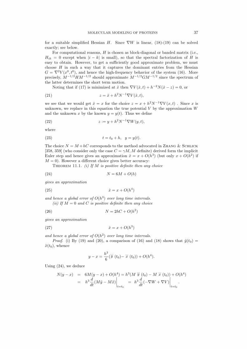
MOLECULAR MODELING OF PROTEINS 37
for a suitable simplified Hessian H. Since ∇W is linear, (18)-(19) can be solvedexactly; see below.
For computational reasons, H is chosen as block-diagonal or banded matrix (i.e.,Hik = 0 except when |i − k| is small), so that the spectral factorization of H iseasy to obtain. However, to get a sufficiently good approximate problem, we mustchoose H in such a way that it captures the dominant entries from the HessianG = ∇2V (x0, t0), and hence the high-frequency behavior of the system (16). Moreprecisely, M−1/2HM−1/2 should approximate M−1/2GM−1/2 since the spectrum ofthe latter determines the short term motion.
Noting that if (17) is minimized at x then ∇V (x, t) + h−2N(x− z) = 0, or
z = x+ h2N−1∇V (x, t),(21)
we see that we would get x = x for the choice z = x + h2N−1∇V (x, t) . Since x isunknown, we replace in this equation the true potential V by the approximation Wand the unknown x by the known y = y(t). Thus we define
z := y + h2N−1∇W (y, t),(22)
where
t = t0 + h, y = y(t).(23)
The choice N = M+hC corresponds to the method advocated in Zhang & Schlick[358, 359] (who consider only the case C = γM,M definite) derived form the implicitEuler step and hence gives an approximation x = x + O(h3) (but only x + O(h2) ifM = 0). However a different choice gives better accuracy:
Theorem 11.1. (i) If M is positive definite then any choice
N = 6M +O(h)(24)
gives an approximation
x = x+O(h4)(25)
and hence a global error of O(h3) over long time intervals.(ii) If M = 0 and C is positive definite then any choice
N = 2hC +O(h2)(26)
gives an approximation
x = x+O(h3)(27)
and hence a global error of O(h2) over long time intervals.Proof. (i) By (19) and (20), a comparison of (16) and (18) shows that y(t0) =
x(t0), whence
y − x =h3
6(...y (t0)− ...
x (t0)) +O(h4).
Using (24), we deduce
N(y − x) = 6M(y − x) +O(h4) = h3(M...y (t0)−M ...
x (t0)) +O(h4)
= h3 d
dt(My −Mx)
∣∣∣∣t=t0
= h3 d
dt(−∇W +∇V )
∣∣∣∣t=t0
.

38 A. NEUMAIER
Now (21) gives
x = z − h2N−1∇V (x, t) = y − h2N−1(∇V (x, t)−∇W (y, t))
= y − h2N−1
(hd
dt(∇V −∇W )
∣∣∣∣t=t0
+O(h2)
)
= y − (−(y − x) +O(h4)) +O(h4) = x+O(h4).
(ii) If M = 0 then (16), (18) and (19) force y(t0) = x(t0) (that can now no longerbe prescribed freely), whence
y − x =h2
2(y(t0)− x(t0)) +O(h3).
Using (26), we deduce
N(y − x) = h3C(y(t0)− x(t0)) +O(h4)
= h3 d
dt(Cy − Cx)
∣∣∣∣t=t0
+O(h4)
= h3 d
dt(−∇w +∇v)
∣∣∣∣t=t0
+O(h4),
and as before we get x = x + O(h3). A power of h is lost since N = O(h). Finally,the statements about the global errors follow along standard lines.
We conjecture that the choice
N = 6M + 2hC(28)
which gives the approximation (25) if M is definite and (27) if M = 0 will be a goodchoice that gives good long time results even in the case of strong damping C À M(when, after rescaling the time, a singularly perturbed version of (ii) results, and thechoice of an arbitrary N with (24) would be accurate only for times of the order ofC−1M).
Note that the theorem is valid for all consistent choices of W ; however, this choiceaffects the time scale on which the asymptotic result is valid. In order to be able to uselarge time steps, ∇2W should account well for all absolutely large eigenvalues of ∇2V ,thus eliminating them from the corrective dynamics handled by the minimization.
We now look at the solution of (18), (19) for the choice
W (y, t) = gT (y − x0) +1
2(y − x0)TH(y − x0),(29)
with a symmetric matrix H, in principle arbitrary but in practice an easily factorizableapproximation to ∇2V (x0, t0). Using a spectral factorization
M−12HM−
12 = QΛQT , QTQ = I, Λ diagonal(30)
and
S := M−12Q,(31)
we have
HS = MSΛ, (MS)−1 = ST .(32)

MOLECULAR MODELING OF PROTEINS 39
Hence multiplication of (29) with ST and use of the new variable u with
y = x0 + Su
reduces the system (18) to the form
u+ Γu+ Λu+ h = 0, h = ST g,
where Γ = STCS. In molecular dynamics simulations, where we have little informa-tion about C anyway, the choice
C = γM(33)
has been repeatedly used in the literature. For this choice, Γ = γI, and we get thedecoupled system
u+ γu+ Λu+ h = 0, h = ST g(34)
that is easy to solve. (For other choices of C, one would need to solve a quadraticeigenvalue problem in place of (30) in order to diagonalize the system, recast in firstorder form.)
In the case of a stochastic differential equation we have
V (x, t) = V (x)− ε(t)T (x− x0),
where
〈ε(t)ε(t)T dt〉 = 2kBT C.
It is then natural to keep this stochastic linear term also in W , thus using g− ε(t) inplace of g. We find in place of h the transformed forcing term
ST (g − ε(t)) = h− η(t)
with a random term η satisfying the relation
〈η(t)η(t)T dt〉 = 〈ST ε(t)ε(t)TSdt〉 = 2kBT STCS.
Hence, assuming again (33), we find
u+ γu+ Λu+ h = η(t), h = ST g,(35)
where
〈η(t)η(t)T dt〉 = 2γkBT I.
Thus the system is again fully decoupled and is easy to solve; for the details seeZhang & Schlick [359].
Using (22) and (23), we find from u = u(t) the vector
z = y + h2N−1(g +H(y − x0)) = y +h2
6 + 2hγM−1(g +HSu).

40 A. NEUMAIER
Hence, using (31) and (32),
z = y +h2
6 + 2hγS(Λu+ h),(36)
and in the stochastic case (35)
z = y +h2
6 + 2hγS(Λu+ h− η(t)).(37)
Since the formulas (34), (36) (or (35), (37) in the stochastic case) no longer dependon H, they remain valid even when only an approximate spectral factorization ofM−1HM−1 (but with orthogonal Q) is used. This is equivalent to using instead ofthe original H the matrix H = MSΛ(MS)T for which the spectral factorization (30)is valid.
Moreover, due to the fact that the matrix S is only used to calculate two matrixvector products, the spectral matrix Q need not be available explicitly. Instead itcan be held as a product of reflections and rotations, as obtained from the cheapereigenvalue calculation. (This is usually done by tridiagonalization and subsequentuse of the implicit QR algorithm; see e.g. Parlett [231]. There is a trade-off be-tween storing the rotations from the QR iteration or recomputing them at the timeof calculating ST g and later again for S(...).) This also assures that the linear map-ping Q determined in this way remains essentially orthogonal even in finite precisionarithmetic.
Appendix 2: Solvation energy and combination rules. We give here somearguments suggesting that by modifying the combination rules for the pair potentialparameters, a large part of the solvation effects can be taken into account automati-cally.
Suppose we have a molecule with coordinate vector x in a solvent whose molecularposition coordinates are part of the vector xsolv. The combined system is governed bya potential Vtot(x, xsolv), and a natural way to eliminate the solvent from considerationis to look at the reduced potential
V (x) := minxsolv
Vtot(x, xsolv).(38)
Thus we assume that at given molecule position, the solvent molecules take the po-sitions at the global minimum of the total energy, which amounts to looking at themolecule in a completely frozen solvent. If we could find a phenomenological de-scription of the reduced potential V (x), the solvent would not need to be consideredexplicitly.
Wesson & Eisenberg [343] suggest that the solvation energy could be ap-proximately modeled by adding to the potential Vmol(x) of the molecule in isolationadditional terms proportional to the surface area exposed to the solvent. We modifyhis approach and argue that it might be feasible to account for much of the solvationenergy by means of suitable corrections to the pair potentials in the force field, andby suitable adjustments of the combination rules for their parameters.
Indeed, suppose we have two atoms i and k with atomic radii Ri and Rk atdistance rik. Seen from the nucleus of atom i, atom k appears under an angle α givenby sin(α/2) = Rk/rik, and the corresponding cone cuts out on the surface of atom i

MOLECULAR MODELING OF PROTEINS 41
a cap of area
Aik = 2πR2i
(1− 1√
1 + (Rk/rik)2
).
Since the total surface area is Ai = 4πR2i , we find
Aik/Ai =1
2
(1− 1√
1 + (Rk/rik)2
)=: µ(rik/Rk)
as an approximation to the surface fraction of atom i excluded by atom k, at leastwhen rik is not large. For large rik, one would have to change µ so that it decaysat least like the inverse 6th power since particles are not expected to have a largerinfluence over large distances.
The total excluded fraction can now be approximated by summing over all atomsk 6= i, and the solvation energy contributed by atom i could be modeled by a multipleof the difference between this sum and 1, hence by
Esolv,i = σi
1−
∑
k 6=iµ
(rikRk
) ,
where σi is the solvation energy of an isolated atom i. Apart from constant termsthat don’t affect forces and energy differences, a natural form for a phenomenologicaltotal solvation energy term is therefore
Esolv = −∑
i
σi∑
k 6=iµ(rik/Rk),(39)
for suitable constants σi and a suitable quickly decaying function µ.
Hydrophilic and hydrophobic behavior. We now show that for a simplemodel situation, a solvation term (39) is indeed sufficient to model hydrophilic andhydrophobic effects. We consider a hypothetical situation where we have atoms oftwo kinds A and B that interact by two-particle forces only, given by a pair potentialW (r). The particles are assumed to have the same unit radius and identical behaviorwith respect to each other, irrespective of their kind. However, their behavior withrespect to the solvent (water) is assumed to be opposite: The A’s are hydrophobic,i.e., a larger excluded surface (less surface exposed to water) decreases the solvationenergy. On the other hand, the B’s are hydrophilic, i.e., a smaller excluded surface(more surface exposed to water) decreases the solvation energy. In our model (39),this is achieved by the choice σi = σA > 0 for hydrophobic atoms and σi = σB < 0for hydrophilic ones. Thus the potential energy (including the solvation terms) is
V =∑
x∈AVA(x) +
∑
x∈BVB(x),(40)
where, for simplicity, A and B now also denote the set of position vectors of atoms oftype A and B, respectively, and
VA(x) =∑
y 6=x
(1
2W (‖y − x‖)− σAµ(‖y − x‖)
),(41)

42 A. NEUMAIER
VB(x) =∑
y 6=x
(1
2W (‖y − x‖)− σBµ(‖y − x‖)
).(42)
Theorem 11.2. In any global minimum configuration,
minx∈A
D(x) ≥ maxx∈B
D(x),(43)
where
D(x) =∑
y 6=xµ(‖y − x‖).
In other words, the hydrophobic atoms occupy the positions with largest values ofD(x).
Proof. Consider a global minimum configuration, and suppose we swap the placesof a single pair of atoms in positions x1 ∈ A and x2 ∈ B. Then the potential (40)changes into a potential
V ′ = V − VA(x1)− VB(x2) + VA(x2) + VB(x1)= V + (VA(x2)− VB(x2))− (VA(x1)− VB(x1))= V − (σA − σB)(D(x2)−D(x1)).
Now σA > 0 > σB and V ′ ≥ V since we started at a global minimum. The formula forV ′ therefore implies that D(x2) ≤ D(x1). Since x1 ∈ A and x2 ∈ B were arbitrary,the theorem follows.
Now if µ(r) is a sufficiently fast decaying function, the dominant contributions toD(x) are those by the atoms closest to the atom at x. Therefore, in a large molecularcluster, D(x) is largest far away from the surface of the molecule and smallest atthe surface. Thus the hydrophobic atoms occupy the interior of the cluster, and thehydrophilic atoms are found at the surface. Thus the simple model correctly predictsthe structure expected from purely qualitative reasoning, and the result still leavesmuch room for the precise form of the solvation potential. Of course, in more complexsituations, various forces compete for their influence on the shape of the cluster, andmay cause modifications of this qualitative picture.
We can give the potential (40) a different interpretation by noting that the solva-tion terms just act as asymmetric corrections to the pair interactions: If we introducethe pair potentials
VAA(r) = W (r)− 2σAµ(r),
VBB(r) = W (r)− 2σBµ(r),
VAB(r) = W (r)− (σA + σB)µ(r),
we can write the total potential in the traditional form
V (x) =∑
i<k
Vik(‖xi − xk‖),

MOLECULAR MODELING OF PROTEINS 43
where
Vik =
{VAA if both atoms i and k are of type A,VBB if both atoms i and k are of type B,VAB otherwise.
Moreover, from the construction, we see that the new pair potentials satisfy thecombination rule
VAB =1
2(VAA + VBB).(44)
In particular, if we think of W (r) as a Lennard-Jones potential (11) and of µ(r) =const · r−6 (a cheap choice for µ; the small-distance singularity does not matter sincethe repulsion term dominates there), then the Vik are also Lennard-Jones potentials,but with modified radii, and with a combination rule different from what we wouldexpect from the unsolvated case. However, this suggests that, by fitting the radii andthe combination rules to experimental data instead of deriving them from geometricconsiderations, we might be able to catch a large part of the solvation energy withoutthe need for explicit solvation energy terms. Essentially we are fitting directly thereduced potential (38) with the data at hand, and for this we need more flexiblecombination rules.
REFERENCES
[1] R. A. Abagyan, Towards protein folding by global energy optimization, FEBS Letters 325(1993), pp. 17–22.
[2] V. I. Abkevich, A. M. Gutin and E. I. Shakhnovich, Free energy landscapes for proteinfolding kinetics: intermediates, traps, and multiple pathways in theory and lattice modelsimulations, J. Chem. Phys. 101 (1994), pp. 6052–6062.
[3] M. P. Allen and D. J. Tildesley, Computer Simulation of Liquids, Oxford Univ. Press,New York 1990.
[4] P. Amara, J. Ma and J. E. Straub, Global minimization on rugged energy landscapes, inGlobal Minimization of Nonconvex Energy Functions: Molecular Conformation and ProteinFolding, P. M. Pardalos et al., eds., Amer. Math. Soc., Providence, RI, 1996, pp. 1–15 .
[5] I. P. Androulakis, C. D. Maranas and C. A. Floudas, Global minimum potential energyconformations of oligopeptides, Manuscript (1995). ([email protected])
[6] F. L. Anet, Inflection points and chaotic behavior in searching the conformation space ofcyclononane, J. Am. Chem. Soc. 112 (1990), pp. 7172–7178.
[7] N. L. Allinger, Y. H. Yuh and J.-H. Lii, Molecular mechanics. The MM3 force field forhydrocarbons. 1–3, J. Amer. Chem. Soc. 111 (1989), pp. 8551–8566, 8566-8575, 8576-8582.
[8] A. W. Appel, An efficient program for many-body simulation, SIAM J. Sci. Stat. Comp. 6(1985), pp. 85–103.
[9] A. C. Atkinson, Developments in the design of experiments, Internat. Statist. Rev., 50 (1982),pp. 161–177.
[10] C. L. Atwood, Optimal and efficient designs of experiments, Ann. Math. Statist., 40 (1969),pp. 1570–1602.
[11] B. M. Axilrod and E. Teller, Interaction of the van der Waals’ type between three atoms,J. Chem. Phys. 11 (1943), pp. 299–300.
[12] L. M. Balbes, S. W. Mascarella and D. B. Boyd, A perspective of modern methods incomputer-aided drug design, in Reviews in Computational Physics, Vol. V, K. B. Lipkowitzand D. B. Boyd, eds., VCH Publ., New York 1994, pp. 337–379.
[13] R. E. Bank, R. Bulirsch, H. Gajewski and K. Merten, eds., Mathematical Modellingand Simulation of Electrical Circuits and Semiconductor Devices, Birkhauser, Basel 1994.
[14] E. Barth, K. Kuczera, B. Leimkuhler and R. D. Skeel, Algorithms for constrainedmolecular dynamics, J. Comp. Chem. 16 (1995), pp. 1192—1209.
[15] E. Barth, M. Mandziuk and T. Schlick, A separating framework for increasing the timestep in molecular dynamics, in Computer Simulation of Biomolecular Systems: Theoreticaland Experimental Applications, W. F. van Gunsteren et al., eds., ESCOM, Leiden, TheNetherlands, 1996 (in press).
44 A. NEUMAIER
[16] G. J. Barton, Protein secondary structure prediction, Curr. Opinion Struct. Biol. 5 (1995),pp. 372–376.
[17] A. Bauer and A. Beyer, An improved pair potential to recognize native protein folds, Pro-teins: Struct. Funct. Gen. 18 (1994), pp. 254–261.
[18] J. F. Bazan, Structural Design and Molecular Evolution of a Cytokine Receptor Superfamily,Proc. Natl. Acad. Sci. USA 87 (1990), pp. 6934–6938.
[19] F. C. Bernstein, T. F. Koetzle, G. J. Williams, E. Meyer, M. D. Bryce, J. R. Rogers,O. Kennard, T. Shikanouchi and M. Tasumi, The protein data bank: A computer-based archival file for macromolecular structures, J. Mol. Biol. 112 (1977), pp. 535–542.
[20] M. Billeter, T. F. Havel and K. Wutrich, The ellipsoid algorithm as a method for thedetermination of polypeptide conformations from experimental distance constraints andenergy minimization, J. Comp. Chem. 8 (1986), pp. 132–141.
[21] M. Bishop and S. Frinks, Error analysis in computer simulations, J. Chem. Phys. 87 (1987),pp. 3675–3676.
[22] A. Bjorck, Solution of equations in IRn, in Handbook of Numerical Analysis, P. G. Ciarletand J. L. Lions, eds., North Holland, Amsterdam 1990, pp. 465–652.
[23] A. Bjorck, Numerical Methods for Least Squares Problems, SIAM, Philadelphia 1996.[24] J. M. Blaney and J. S. Dixon, Distance geometry in molecular modeling, in Reviews in
Computational Physics, Vol V, K. B. Lipkowitz and D. B. Boyd, eds., VCH Publ., NewYork 1994.
[25] J. A. Board, J. W. Causey, T. F. Leathrum Jr., A. Windemuth and K. Schulten, Ac-celerated molecular dynamics simulation with the parallel fast multipole algorithm, Chem.Phys. Lett. 198 (1992), pp. 89–94.
[26] B. Borstnik, D. Pumpernik, D. Janezic and A. Azman, Molecular dynamics studiesof molecular interactions, Chapter 7 in Molecular Interaction, H. Ratajczak and W. J.Orville-Thomas, eds., Wiley, New York 1980.
[27] G. Bossis, B. Quentrec and J. P. Boon, Brownian dynamics and the fluctuation-dissipationtheorem, Mol. Phys. 45 (1982), pp. 191–196.
[28] J. P. Bowen and N. L. Allinger, Simplified models for understanding and predicting proteinstructure, in Reviews in Computational Chemistry, Vol. II, K. B. Lipkowitz and D. B. Boyd,eds., VCH Publ., New York 1991, pp. 57–80.
[29] J. U. Bowie and D. Eisenberg, Inverted protein structure prediction, Curr. Opinion Struct.Biol. 3 (1993), pp. 437–444.
[30] C. Branden and J. Tooze, Introduction to Protein Structure, Garland, New York 1991.[31] K. E. Brenan, S. L. Campbell and L. R. Petzold, Numerical Solution of Initial Value
Problems in Differential-Algebraic Equations, North-Holland, New York 1989.[32] T. Brodmeier and E. Pretsch, Application of genetic algorithms in molecular modeling, J.
Comp. Chem. 15 (1994), pp. 588–595.[33] B. R. Brooks, R. Bruccoleri, B. Olafson, D. States, S. Swaminathan and M.
Karplus, CHARMM: a program for macromolecular energy, minimization, and dynamicscalculations, J. Comp. Chem. 4 (1983), pp. 187–217.
[34] C. L. Brooks, M. Karplus and B. M. Pettitt, Proteins: a Theoretical Perspective ofDynamics, Structure, and Thermodynamics, Adv. Chem. Phys. 71, Wiley, New York 1988.
[35] A. Brunger, C. B. Brooks and M. Karplus, Stochastic boundary conditions for moleculardynamics simulations of ST2 water, Chem. Phys. Lett. 105 (1982), pp. 495–500.
[36] A. T. Brunger, J. Kuriyan and M. Karplus, Crystallographic R factor refinement bymolecular dynamics, Science 235 (1987), pp. 458.
[37] U. Burkert and N. L. Allinger, Molecular Mechanics, Amer. Chem. Soc., Washington,D. C. 1982.
[38] L. J. Buturovic, T. F. Smith and S. Vajda, Finite-state and reduced-parameter represen-tations of protein backbone conformations, J. Comp. Chem. 15(1994), pp. 300–312.
[39] R. H. Byrd, E. Eskow, R. B. Schnabel and S. L. Smith, Parallel global optimization:numerical methods, dynamic scheduling methods, and applications to molecular configu-ration, in Parallel Computation, B. Ford and A. Fincham (eds.), Oxford University Press,1993, pp. 187–207.
[40] R. H. Byrd, E. Eskow, A. van der Hoek, R. B. Schnabel and K. B. Oldenkamp, Aparallel global optimization method for solving molecular cluster and polymer conformationproblems, in Proc. 7th SIAM Conf. Parallel Processing Sci. Comput., SIAM, 1995, pp. 72–77.
[41] R. H. Byrd, E. Eskow, A. van der Hoek, R. B. Schnabel, C.-S. Shao and Z. Zou, Globaloptimization methods for protein folding problems, in Global Minimization of NonconvexEnergy Functions: Molecular Conformation and Protein Folding, P. M. Pardalos et al.,

MOLECULAR MODELING OF PROTEINS 45
eds., Amer. Math. Soc., Providence, RI, 1996, pp. 29–39.[42] A. Caflisch and M Karplus, Molecular dynamics studies of protein and peptide folding and
unfolding, Chapter 7 in The Protein Folding Problem and Tetiary Structure Prediction, K.Merz et al., eds, Birkhauser, Boston 1994.
[43] C. J. Camacho and D. Thirumalai, Minimum energy compact structures of random se-quences of heteropolymers, Phys. Rev. Lett. 71 (1993), pp. 2505–2508.
[44] C. R. Cantor and P. R. Schimmel, Biophysical Chemistry, Freeman, New York 180.[45] G. Casari and M. J. Sippl, Structure-derived hydrophobic potential, J. Mol. Biol. 224 (1992),
pp. 725–732.[46] H. F. Chan and K. A. Dill, Origins of structure in globular proteins, Proc. Natl. Acad. Sci.
USA 87 (1990), pp. 6388–6392.[47] H. F. Chan and K. A. Dill, Polymer principles in protein structure and stability, Ann. Rev.
Biophys. Chem. 20 (1991), pp. 447–490.[48] H. F. Chan and K. A. Dill, The protein folding problem, Physics Today (February 1993),
pp. 24–32.[49] C. Chen, Y. Zhu, J. A. King and L. B. Evans, A molecular thermodynamic approach to
predict the secondary structure of homopolypeptides in aqueous systems, Biopolymers 32(1992), pp. 1375–1392.
[50] G. Ciccotti, D. Frenkel and I. R. McDonald, Simulation of Liquids and Solids: Molec-ular Dynamics and Monte Carlo Methods in Statistical Mechanics, North-Holland Ams-terdam 1987.
[51] G. Ciccotti, and J. P. Ryckaert, On the derivation of the generalized Langevin equationfor interacting Brownian particles, J. Stat. Phys. 26 (1981), pp. 73–82.
[52] M. Clark, R. D. Cramer III and N. van Opdenbosch, Validation of the general purposeTripos 5.2 force field, J. Comput. Chem. 10 (1989), pp. 982–1012.
[53] T. Clark, A Handbook of Computational Chemistry: A Practical Guide to Chemical Structureand Energy Calculations, Wiley-Interscience, New York 1985.
[54] F. E. Cohen, L. M. Gregoret, S. R. Presnell and I. D. Kuntz, Theoretical approachesto protein structure prediction, in Protein Folding, L. M. Gierasch and J. King, eds., Amer.Ass. Adv. Sci., Washington 1990, pp. 251–258.
[55] T. Coleman, D. Shalloway and Z. Wu, A parallel build-up algorithm for global energyminimizations of molecular clusters using effective energy simulated annealing, J. GlobalOptim. 4 (1994), pp. 171–186.
[56] M. L. Conolly, Molecular surfaces: a review, Network Science, April 1996.(http://www.awod.com/netsci/Issues/Apr96/feature1.html)
[57] J. H. Conway, T. D. Duff, R. H. Hardin and N. A. Sloane, Minimal-energy clusters ofhard spheres, Discr. Comput. Geom., to appear.
[58] W. D. Cornell, P. Cieplak, C. I. Bayly, I. R. Gould, K. M. Merz, D. M. Ferguson,D. C. Spellmeyer, T. Fox, J. W. Caldwell and P. A. Kollmann, A second gen-eration force field for the simulation of proteins, nucleic acids, and organic molecules, J.Amer. Chem. Soc. 117 (1995), pp. 5179–5197.
[59] D. G. Covell and R. L. Jernigan, Conformations of folded proteins in restricted spaces,Biochemistry 29 (1990), pp. 3287–3294.
[60] C. J. Cramer and D. G. Truhlar, Continuum solvation models: classical and quantummechanical implementations, in Reviews in Computational Chemistry, Vol. VI, K. B. Lip-kowitz and D. B. Boyd, eds., VCH Publ., New York 1995, pp. 1–72.
[61] I. P. Crawford, T. Niermann and K. Kirschner, Predictions of secondary structure byevolutionary comparison: Application to the alpha subunit of tryptophan synthase, Pro-teins: Struct. Funct. Gen. 1 (1987), pp. 118–129.
[62] T. E. Creighton, Proteins. Structure and Molecular Principles, Freeman, New York 1984.[63] T. E. Creighton, Understanding protein folding pathways and mechanisms, in Protein Fold-
ing, L. M. Gierasch and J. King, eds., Amer. Ass. Adv. Sci., Washington 1990, pp. 157–170.[64] G. M. Crippen, Chemical distance geometry: current realization and future projection, J.
Math. Chem. 6 (1991), pp. 307–324.[65] G. M. Crippen, Distance Geometry and Conformational Calculations, Wiley, New York 1981.[66] G. M. Crippen and T. F. Havel, Distance Geometry and Molecular Conformation, Wiley,
New York 1988.[67] G. M. Crippen and M. E. Snow, A 1.8 A resolution potential function for protein folding,
Biopolymers 29 (1990), pp. 1479–1489.[68] P. Culot, G. Dive, V. H. Nguyen and J. M. Ghuysen, A quasi-Newton algorithm for first
order saddle point location, Theor. Chim. Acta 82 (1992), pp. 189–205.[69] V. Daggett and M. Levitt, Protein unfolding pathways explored through molecular dynam-

46 A. NEUMAIER
ics simulations, J. Mol. Biol. 232 (1993), pp. 600–619.[70] T. Darden, D. York and L. Pedersen, Particle mesh Ewald: An N · log(N) method for
Ewald sums in large systems, J. Chem Phys. 98 (1993), pp. 10089–10092.[71] P. Dauber-Osguthorpe and D. J. Osguthorpe, Partitioning the motion in molecular
dynamics simulations into characteristic modes of motion, J. Comp. Chem. 14 (1993),pp. 1259–1271.
[72] P. Dauber-Osguthorpe, V. A. Roberts, D. J. Osguthorpe, J. Wolff, M. Genest andA. T. Hagler, Proteins: Struct. Funct. Gen. 4 (1988), pp. 31.
[73] L. Davis, ed., Handbook of Genetic Algorithms, van Nostrand Reinhold, New York 1991.[74] J. E. Dennis and R. B. Schnabel, Numerical Methods for Unconstrained Optimization and
Nonlinear Equations, Classics in Applied Math. 16, SIAM, Philadelphia 1996.[75] P. Derreumaux, and G. Vergoten, Influence of the Spectroscopic Potential Energy Func-
tion SPASIBA on Molecular Dynamics of Proteins: Comparison with the AMBER Poten-tial, J. Mol. Struct. 286 (1993), pp. 55–64.
[76] P. Derreumaux, G. Zhang, T. Schlick and B. Brooks, A truncated Newton minimizeradapted for CHARMM and biomolecular applications, J. Comp. Chem. 15 (1994), pp. 532–552.
[77] J. M. Deutch and I. Oppenheim, Molecular theory of Brownian motion for several particles,J. Chem. Phys. 54 (1971), pp. 3547–3555.
[78] K. A. Dill, S. Bromberg, K. Yue, K. M. Fiebig, D. P. Yee, P. D. Thomas and H. S.Chan, Principles of protein folding - a perspective from simple exact models, ProteinScience 4 (1995), pp. 561–602.
[79] K. A. Dill, A. T. Phillips and J. B. Rosen, Molecular structure prediction by globaloptimization, Manuscript (1996). ([email protected])
[80] U. Dinur and A. T. Hagler, New approaches to empirical force fields, in Reviews in Compu-tational Chemistry, Vol. II, K. B. Lipkowitz and D. B. Boyd, eds., VCH Publ., New York1991, pp. 99–164.
[81] C. M. Dobson, Unfolded proteins, compact states and molten globules, Curr. Opinion Struct.Biol. 2 (1992), pp. 6–12.
[82] S. Dosanjh and W. J. Camp, Computational design of materials: Part II, SIAM News,May/June 1994, 10–11.
[83] N. Draper and H. Smith, Applied Regression Analysis, 2nd ed., Wiley, New York 1981.[84] R. L. Dunback and M. Karplus, Backbone-dependent rotamer library for proteins. Appli-
cation to side-chain prediction, J. Mol. Biol. 230 (1993), pp. 543–574.[85] R. L. Dunback and M. Karplus, Conformational analysis of the backbone-dependent ro-
tamer preferences of protein sidechains, Struct. Biol. 1 (1994), pp. 334–340.[86] J. D. Dunitz, H. Eser, M. Bixon and S. Lifson, Die Strukturen der mittleren
Ringverbindungen XII - XIII, Helvetica Chimica Acta 50 (1967), pp. 1565–1572; 1572-1583.
[87] Y. K. Edwards and S. J. Perkins, The protein fold of the von Willebrand factor type Ais predicted to be similar to the open twisted beta-sheet flanked by alpha-helices found inhuman ras-p21, FEBS Letters 358 (1995), pp. 283–286.
[88] J. E. Eksterowicz and K. N. Houk, Transition state modeling with empirical force fields,Chem. Rev. 93 (1993),2439–2461.
[89] R. Elber and M. Karplus, Multiple conformational states of proteins: a molecular dynamicsanalysis of myoglobin, Science 235 (1987), pp. 318–321.
[90] R. A. Engh and R. Huber, Accurate bond and angle parameters for X-ray protein structurerefinement, Acta Cryst. A47 (1991), pp. 392–400.
[91] U. Eßmann, L. Perera, M. L. Berkowitz, T. Darden, H. Lee and L. G. Pedersen, Asmooth particle mesh Ewald method, J. Chem. Phys., to appear.
[92] P. Ewald, Ann. Phys. 64 (1921), pp. 253.[93] L. Farnell, W. G. Richards and C. R. Ganellin, Calculation of conformational free
energy of histamine, J. Theor. Biol. 43 (1974), pp. 389–392.[94] V. V. Fedorov, Theory of Optimal Experiments, Acad. Press, London 1972.[95] D. M. Ferguson, A. Marsh, T. Metzger, D. Garrett and K. Kastella, Conformational
searches for the global minimum of protein models, J. Global Optim. 4 (1994), pp. 209–227.[96] J. S. Fetrow and S. H. Bryant, New programs for protein tertiary structure prediction,
Biotechnology 11 (1993), pp. 479–484.[97] R. Fletcher, Practical Methods of Optimization, Wiley, New York 1987.[98] G. Fogarasi and P. Pulay, Ab initio calculation of force fields and vibrational spectra, in
Vibrational Spectra and Structure, Vol. 14, J. R. Durig, ed., Elsevier, Amsterdam 1985,pp. 125–219.
MOLECULAR MODELING OF PROTEINS 47
[99] S. Fortier, I. Castleden, J. Glasgow, D. Conklin, C. Walmsley, L. Leherte andF. A. Allen, Molecular scene analysis: the integration of direct-method and artificial in-telligence strategies for solving protein crystal structures, Acta Cryst. D49 (1993), pp. 168–178.
[100] M. S. Friedrichs, R. A. Goldstein and P. G. Wolynes, Generalized protein tertiarystructure recognition using associative memory Hamiltonians, J. Mol. Biol. 222 (1991),pp. 1013–1034.
[101] H. Frohlich, Theory of Dielectrics, Clarendon Press, Oxford 1958.[102] K. Fukunaga, Introduction to Statistical Pattern Recognition, 2nd ed., Academic Press, Lon-
don 1990.[103] C. W. Gardiner, Handbook of Stochastic Methods, Springer, Berlin 1985.[104] J. Garnier, Protein structure prediction, Biochimie 72 (1990), pp. 513–524.[105] D. L. Gerloff, G. Chelvanayagam and S. A. Benner, A predicted consensus structure
for the protein-kinase c2 homology (c2h) domain, the repeating unit of synaptotagmin,Proteins: Struct. Funct. Gen. 22 (1995), pp. 299–310.
[106] C. Giacovazzo, ed., Fundamendals of Crystallography, Oxford Univ. Press, Oxford 1985.[107] J. Gibrat, J. Garnier and N. Go, Normal mode analysis of oligomeric proteins: reduction
of the memory requirements by consideration of rigid geometry and molecular symmetry,J. Comp. Chem. 15 (1994), pp. 820–837.
[108] J. Gibrat, J. Garnier and B. Robson, Further developments of secondary structure pre-dictions using information theory: new parameters and consideration of residue pairs, J.Mol. Biol. 198 (1987), pp. 425–443.
[109] K. D. Gibson and H.. A. Scheraga, Desicions in force field development. Reply to Kollmanand Dill, J. Biomol. Struct. Dyn. 8 (1991), pp. 1109–1111.
[110] L. M. Gierasch and J. King, Protein Folding: Deciphering the Second Half of the GeneticCode, Amer. Ass. Advancement Sci., 1990.
[111] T. L. Gilbert, Soft-sphere model for closed-shell atoms and ions, J. Chem. Phys. 49 (1968),pp. 2640–2642.
[112] P. E. Gill, W. Murray and M. H. Wright, Practical Optimization, Acad. Press, London1981.
[113] M. K. Gilson, K. A. Sharp and B. H. Honig, Calculating the electrostatic potential ofmolecules in solution: methods and error assessment, J. Comput. Chem. 9 (1987), pp. 327–335.
[114] A. Godzik, A. Kolinski and J. Skolnick, Topology fingerprint approach to the inversefolding problem, J. Mol. Biol. 227 (1992), pp. 227–238.
[115] A. Godzik, A. Kolinski and J. Skolnick, De novo and inverse folding predictions of proteinstructure and dynamics, J. Computer-Aided Mol. Des. 7 (1993), pp. 397–438.
[116] A. Godzik, A. Kolinski and J. Skolnick, Lattice representations of globular proteins: Howgood are they?, J. Comp. Chem. 14 (1993), pp. 1194–1202.
[117] R. A. Goldstein, Z. A. Luthey-Schulten and P. G. Wolynes, The statistical mechanicalbasis of sequence alignment algorithms for protein structure recognition, Manuscript, 1993.
[118] N. Go and H. A. Scheraga, Analysis of the contribution of internal vibrations to the statis-tical weights of equilibrium conformations of macromolecules, J. Chem. Phys. 51 (1969),pp. 4751–4767.
[119] S. K. Gray, D. W. Noid and B. G. Sumpter, Symplectic integrators for large-scale molec-ular dynamics simulations: A comparison of several explicit methods, J. Chem. Phys. 101(1994), pp. 4062–4072.
[120] L. Greengard and V. Rokhlin, The rapid evaluation of potential fields in three dimensions,in Vortex Methods, C. Anderson and C. Greengaard, eds., Lecture Notes in Math., Springer1988, pp. 121–141.
[121] A. Greiner, W. Strittmatter and J. Honerkamp, Numerical integration of stochasticdifferential equations, J. Statist. Phys. 51 (1988), pp. 95–108.
[122] T. Gund and P. Gund, Three-dimensional molecular modeling by computer, Chapter 10 inMolecular Structure and Energetics, J. F. Liebman and A. Greenberg, eds., Vol. 4 (1987),pp. 319–340.
[123] J. R. Gunn, A. Monge, R. A. Friesner and C. H. Marshall, Hierarchical algorithm forcomputer modeling of protein tertiary structure: folding of myoglobin to 6.2A resolution,J. Phys. Chem. 98 (1994), pp. 702–711.
[124] Z. Guo, D. Thirumalai and J. D. Honeycutt, Folding kinetics of proteins: A model study,J. Chem. Phys. 97 (1992), pp. 525–535.
[125] P. Hanggi, P. Talkner and M. Borkovec, Reaction-rate theory: fifty years after Kramers,Rev. Mod. Phys. 62 (1990), pp. 251–341.

48 A. NEUMAIER
[126] A. T. Hagler, D. J. Osguthorpe, P. Dauber-Osguthorpe and J. C. Hempel, Dynamicsand conformational energetics of a peptide hormone: Vasopressin, Science 227 (1985),pp. 1309–1315.
[127] E. Hairer, C. Lubich and M. Roche, The Numerical Solution of Differential-AlgebraicSystems by Runge-Kutta Methods, Lecture Notes in Math. 1409, Springer, Berlin 1989.
[128] E. Hairer, S. P. Norsett and G. Wanner, Solving Ordinary Differential Equations I, 2ndrev. ed., Springer, Berlin 1993.
[129] E. Hairer and G. Wanner, Solving Ordinary Differential Equations II, Springer, Berlin1991.
[130] E. Hansen, Global Optimization Using Interval Analysis, Dekker, New York 1992.[131] M.-H. Hao and S. C. Harvey, Analyzing the normal mode dynamics of macromolecules by
the component synthesis method, Biopolymers 32 (1992), pp. 1395–1405.[132] M.-H. Hao and H. A. Scheraga, Statistical thermodynamics of protein folding: sequence
dependence, J. Phys. Chem. 98 (1994), 9882-9893.[133] T. Head-Gordon and F. H. Stillinger, Predicting polypeptide and protein structures from
amino acid sequence: antlion method applied to melittin, Biopolymers 33 (1993), pp. 293–303.
[134] T. Head-Gordon, F. H. Stillinger and J. Arrecis, A strategy for finding classes ofminima on a hypersurface: implications for approaches to the protein folding problem,Proc. Natl. Acad. Sci. USA 88 (1991), pp. 11076–11080.
[135] T. Head-Gordon, F. H. Stillinger, M. H. Wright and D. M. Gay, Poly(L-alanine)as a universal reference material for understanding protein energies andstructures, Proc. Natl. Acad. Sci. USA 89 (1992), pp. 11513–11517.
[136] M. Hendlich, P. Lackner, S. Weitckus, H. Floeckner, R. Froschauer, K. Gotts-bacher, G. Casari and M. J. Sippl, Identification of native protein folds amongst alarge number of incorrect models, J. Mol. Biol. 216 (1990), pp. 167–180.
[137] W. A. Hendrickson, Methods Encymol. 115 (1985), pp. 252–270.[138] D. M. Hirst, A Computational Approach to Chemistry, Blackwell Sci. Publ., Oxford 1990.[139] M. R. Hoare, Structure and dynamics of simple microclusters, Adv. Chem. Phys. 40 (1979),
pp. 49–135.[140] M. R. Hoare and J. A. McInnes, Morphology and statistical statics of simple microclusters,
Adv. Phys. 32 (1983), pp. 791–821.[141] U. Hobohm, M. Scharf, R. Schneider and C. Sander, Selection of representative protein
data sets, Protein Sci. 1 (1992), pp. 409–417.[142] C. Hoheisel, Theoretical Treatment of Liquids and Liquid Mixtures, Elsevier, Amsterdam
1993.[143] J. Holland, Genetic algorithms and the optimal allocation of trials, SIAM J. Computing 2
(1973), pp. 88–105.[144] L. Holley and M. Karplus, Protein secondary structure prediction with a neural network,
Proc. Natl. Acad. Sci. USA 86 (1989), pp. 152–156.[145] J. Honerkamp, Stochastic Dynamical Systems: Concepts, Numerical Methods, Data Analysis,
VCH, New York 1994.[146] J. D. Honeycutt and D. Thirumalai, The nature of folded states of globular proteins,
Biopolymers 32 (1992), pp. 695–709.[147] B. Honig and A. Nicholls, Classical electrostatics in biology and chemistry, Science 268
(1995), pp. 1144–1149.[148] A. J. Hopfinger and R. A. Pearlstein, Molecular mechanics force-field parametrization
procedures, J. Comput. Chem. 5 (1984), pp. 486–499.[149] Q. X. Hua, M. Kochoyan and M. A. Weiss, Structure and dynamics of despentapeptide-
insulin in solution: the molten globule hypothesis, Proc. Natl. Acad. Sci. USA 89 (1992),pp. 2379–2383.
[150] Q. X. Hua, J. E. Ladbury and M. A. Weiss, Dynamics of a monomeric insulin analogue:testing the molten globule hypothesis, Biochemistry 32 (1993), pp. 1433–1442.
[151] A. Iniesta and J. G. de la Torre, A second-order algorithm for the simulation of theBrownian dynamics of macromolecular models, J. Chem. Phys. 92 (1990), pp. 2015–2018.
[152] G. Iori, E. Marinari and G. Parisi, Heteropolymer folding on a APE-100 supercomputer,Int. J. Mod. Phys. C 4 (1993), pp. 1333–1341.
[153] A. Irback, C. Peterson and F. Potthast, Identification of amino acid sequences withgood folding properties, Phys. Rev. E, submitted, 1996.
[154] A. Irback and F. Potthast, Studies of an off-lattice model for protein folding: sequencedependence and improved sampling at finite temperature, J. Chem. Phys. 103 (1995),pp. 10298
MOLECULAR MODELING OF PROTEINS 49
[155] IUPAC-IUP Commission on Biochemical Nomenclature, Abbreviations and symbols forthe description of the conformation of polypeptide chains, Biochemistry 9 (1970), pp. 3471–3479.
[156] R. Jaenicke, Protein folding: local structures, domains, subunits, and assemblies, Biochem-istry 30 (1991), pp. 3147–3161.
[157] O. Jardetzky and A. N. Lane, Determination of the solution structure of proteins fromNMR, in Physics of NMR Spectroscopy in Biology and Medicine, B. Maraviglia, ed., NorthHolland, Amsterdam 1988, pp. 267–301.
[158] M. S. Johnson, N. Srinivasan, R. Sowdhamini and T. L. Blundell, Knowledge-basedprotein modeling, Crit. Rev. Biochem. Mol. Biol. 29 (1994), pp. 1–68.
[159] D. Jones and J. Thornton, Protein fold recognition, J. Comput. Aided Mol. Design 7 (1993)439–456.
[160] W. Kabsch, A discussion of the solution for the best rotation to relate two sets of vectors,Acta Cryst. A34 (1978), pp. 827–828.
[161] H. S. Kang, N. A. Kurochkina and B. Lee, Estimation and use of protein backbone angleprobablilities, J. Mol. Biol. 229 (1993), pp. 448–460.
[162] I. G. Kaplan, Theory of Molecular Interactions, Elsevier, Amsterdam 1986.[163] M. Karplus, A. Caflish, A. Sali and E. Shaknovich, Protein dynamics: from the na-
tive to the unfolded state and back again, in Proc. Int. Conf. Mol. Struct. Biol. Vienna,September 17–20, 1995, A. J. Kungl. et al., eds., Gesellschaft Osterreichischer Chemiker,Wien 1995, pp. 129–155.
[164] H.Kawai, T.Kikuchi and Y. Okamoto, A prediction of tertiary structures of peptide by theMonte Carlo simulated annealing method, Protein Eng. 3 (1989), pp. 85–94.
[165] T. Kihara and S. Ichimaru, Intermolecular Forces, Wiley, Chichester 1978.[166] S. Kirkpatrick, C. D. Geddat, Jr., and M. P. Vecchi, Optimization by simulated an-
nealing, Science 220 (1983), pp. 671–680.[167] P. E. Kloeden and E. Platen, Numerical Solution of Stochastic Differential Equations,
Springer, Berlin 1992.[168] P. E. Kloeden, E. Platen and H Schurz, Numerical Solution of SDE Through Computer
Experiments, Springer, Berlin 1994.[169] D. Kneller, F. Cohen and R. Langridge, Improvements in protein secondary structure
predictions by an enhanced neural network, J. Mol. Biol. 214 (1990), pp. 171–182.[170] H. Koppen, The use of supercomputers in medical chemistry. Examples from peptide and
protein projects, in Supercomputer and Chemistry, U. Harms, ed., Springer, Berlin 1990,pp. 99–113.
[171] A. Kolinski, A. Godzik and J. Skolnick, A general method for the prediction of the threedimensional structure and folding pathway of globular proteins: application to designedhelical proteins, J. Chem. Phys. 98 (1993), pp. 7420–7433.
[172] J. Kostrowicki, L. Piela, B. J. Cherayil and H. Scheraga, Performance of the diffusionequation method in searches for optimum structures of clusters of Lennard-Jones atoms,J. Phys. Chem. 95 (1991), pp. 4113–4119.
[173] J. Kostrowicki and H. A. Scheraga, Application of the diffusion equation method forglobal optimization to oligopeptides, J. Phys. Chem. 96 (1992), pp. 7442–7449.
[174] J. Kostrowicki and H. A. Scheraga, Some approaches to the multiple-minima problem inprotein folding, in Global Minimization of Nonconvex Energy Functions: Molecular Con-formation and Protein Folding, P. M. Pardalos et al., eds., Amer. Math. Soc., Providence,RI, 1996, pp. 123–132.
[175] S. Krimm, Spectra and structure of polypeptides, in Vibrational Spectra and Structure, Vol.16, J. R. Durig, ed., Elsevier, Amsterdam 1987, pp. 1–72.
[176] B. M. Ladanyi and M. S. Skaf, Computer simulation of hydrogen-bonding liquids, Ann.Rev. Phys. Chem. 44 (1993), pp. 335–368.
[177] M. Lambert and H. Scheraga, Pattern recognition in the prediction of protein structure,I-III, J. Comp. Chem. 10 (1989), pp. 770–797; 798-816; 817-831.
[178] E. S. Lander and M. S. Waterman, Calculating the Secrets of Life: Contributions of theMathematical Sciences to Molecular Biology, National Academic Press, Washington, D. C., 1995.
[179] R. H. Lathrop and T. F. Smith, Global optimum protein threading with gapped alignmentand empirical pair score functions, J. Mol. Biol., 1996 (in press).
[180] A. R. Leach, A survey of methods for searching the conformational space of small andmedium-sized molecules, in Reviews in Computational Chemistry, Vol. II, K. B. Lipkowitzand D. B. Boyd, eds., VCH Publ., New York 1991, pp. 1–55.
[181] T. Lee, D. M. York and W. Yang, A new definition of atomic charges based on a variational
50 A. NEUMAIER
principle for the electrostatic potential energy, J. Chem. Phys. 102 (1995), pp. 7549–7556.[182] C. Lee and S. Subbiah, Prediction of protein side-chain conformation by packing optimiza-
tion, J. Mol. Biol. 217 (1991), pp. 373–388.[183] S. L. Le Grand and K. M. Merz jr., The application of the genetic algorithm to the
minimization of potential energy functions, J. Global Optim. 3 (1993), pp. 49–66.[184] C. M. -R. Lemer, M. J. Rooman and S. J. Wodak, Protein structure prediction by thread-
ing methods: evaluation of current techniques, Proteins: Struct. Funct. Gen. 23 (1995),pp. 337–355.
[185] P. E. Leopold, M. Montal and J. N. Onuchic, Protein folding funnels: a kinetic approachto the sequence-structure relationship, Proc. Natl. Acad. Sci. USA 89 (1992), pp. 8721–8725.
[186] C. Levinthal, Are there pathways to protein folding? J. Chim. Phys. 65 (1968), pp. 44–45.[187] M. Levitt, C. Sander and P. S. Stern, Protein normal-mode dynamics: trypsin inhibitor,
crambin, ribonuclease and lysozyme, J. Mol. Biol. 181 (1985), pp. 423–447.[188] R. M. Levy, R. P. Sheridan, J. W. Keepers, G. S. Dubey, S. Swaminathan and M.
Karplus, Molecular dynamics of myoglobin at 298oK, Biophys. J. 48 (1985), pp. 509–518.[189] Z. Li and H. A. Scheraga, Monte Carlo approach to the multiple-minima problem in protein
folding, Proc. Natl. Acad. Sci. USA 84 (1987), pp. 15–29.[190] S. Lifson, Potential energy functions for structural molecular biology, in Supramolecular
Structure and Function, G. Pifat and J. N. Herak, eds., Plenum, New York 1983, pp. 1–44.[191] K. B. Lipkowitz and D. B. Boyd, eds., Reviews in Computational Chemistry, Vol. I-VII,
VCH Publ., New York 1990–1996.[192] J. Ma and J. E. Straub, Simulated annealing using the classical density distribution, J.
Chem. Phys. 101 (1994), pp. 533–541.[193] R. Marz, Numerical methods for differential-algebraic equations, in Acta Numerica 1992, A.
Iserles, ed., Cambridge Univ. Press 1992, pp. 141–198.[194] V. N. Maiorov and G. M. Crippen, Contact potential that recognizes the correct folding of
globular proteins, J. Mol. Biol. 227 (1992), pp. 876–888.[195] G. C. Maitland, M. Rigby, E. B. Smith and W. A. Wakeham, Intermolecular Forces.
Their Origin and Determination, Clarendon Press, Oxford 1981.[196] J. R. Maple, M.-J. Hwang, T. P. Stockfisch, U. Dinur, M. Waldman, C. S. Ewing
and A. T. Hagler, Derivation of Class II Force Fields. I. Methodology and QuantumForce Field for the Alkyl Functional Group and Alkane Molecules, J. Comput. Chem. 15(1994), pp. 162–182.
[197] C. D. Maranas and C. A. Floudas, A global optimization approach for Lennard-Jonesmicroclusters, J. Chem. Phys. 97 (1992), pp. 7667–7678.
[198] C. D. Maranas and C. A. Floudas, Global minimum potential energy conformations ofsmall molecules, J. Global Optim. 4 (1994), pp. 135–170.
[199] C. D. Maranas and C. A. Floudas, A deterministic global optimization approach for molec-ular structure determination, J. Chem. Phys. 100 (1994), pp. 1247–1261.
[200] C. D. Maranas, I. P. Androulakis and C. A. Floudas, A deterministic global optimiza-tion approach for the protein folding problem, in Global Minimization of Nonconvex EnergyFunctions: Molecular Conformation and Protein Folding, P. M. Pardalos et al., eds., Amer.Math. Soc., Providence, RI, 1996, pp. 133–150.
[201] P. Matstoms, Sparse QR Factorization in MATLAB, ACM Trans. Math. Software 20 (1994),pp. 136–159.
[202] J. A. McCammon and S. C. Harvey, Dynamics of Proteins and Nuclein Acids, CambridgeUniv. Press, Cambridge 1987.
[203] J. A. McCammon and M. Karplus, Simulation of protein dynamics, Ann. Rev. Phys. Chem.31 (1980), pp. 29–45.
[204] M. L. McKee and M. Page, Computing reaction pathways on molecular potential energysurfaces, in Reviews in Computational Physics, Vol. IV, K. B. Lipkowitz and D. B. Boyd,eds., VCH Publ., New York 1993, pp. 337–379.
[205] P. G. Mezey, Potential Energy Hypersurfaces, Elsevier, Amsterdam 1987.[206] S. Miyazawa and R. L. Jernigan, Protein Eng. 6 (1993), pp. 267–278.[207] A. D. Miranker and C. M. Dobson, Collapse and cooperativity in protein folding, Curr.
Opinion Struct. Biol. 6 (1996), pp. 31–42.[208] S. Miyamoto and P. A. Kollman, SETTLE: An analytic version of the SHAKE and RAT-
TLE algorithm for rigid water models, J. Comp. Chem. 13 (1992), pp. 952–962.[209] J. Mockus, Bayesian Approach to Global Optimization, Kluwer, Dordrecht 1989.[210] F. A. Momany, R. F. McGuire, A. W. Burgess and H. A. Scheraga, Energy parameters
in polypeptides. VIII, J. Phys. Chem. 79 (1975), pp. 2361–2381.[211] F. A. Momany, V. J. Klimkowski and L. Schafer, On the use of conformationally depen-
MOLECULAR MODELING OF PROTEINS 51
dent geometry trends from ab initio dipeptide studies to refine potentials for the empiricalforce field CHARMM, J. Comp. Chem. 11 (1990), pp. 654–662.
[212] F. Momany, R. McGuire, A. Burgess and H. Scheraga, Energy parameters in polypep-tides VII, J. Phys. Chem. 79 (1975), pp. 2361–2381.
[213] A. Monge, R. A. Friesner and B. Honig, An algorithm to generate low-resolution proteintertiary structures from knowledge of secondary structure, Proc. Natl. Acad. Sci. USA 91(1994), pp. 5027–5029.
[214] J. J. More and Z. Wu, Global continuation for distance geometry problems, Manuscript(1995). ([email protected])
[215] J. J. More and Z. Wu, Smoothing techniques for macromolecular global optimization,Manuscript (1995). ([email protected])
[216] B. T. Nall and K. A. Dill, Conformations and Forces in Protein Folding, Amer. Ass. Adv.Sci., Washington 1991.
[217] S. G. Nash, Preconditioning of truncated Newton methods, SIAM J. Sci. Statist. Comp. 6(1985), pp. 599–616.
[218] National Research Council, Mathematical Challenges From Theoretical/ComputationalChemistry, National Academy Press, Washington, D. C. 1995. (available via the WorldWide Web, http://www.nas.edu)
[219] G. Nemethy, K. D. Gibson, K. A. Palmer, C. N. YoonG. Paterlini, A. Zagari, S.Rumsey and H. A. Scheraga, Energy parameters in polypeptides. 10. Improved geo-metrical parameters and nonbonded interactions for use in the ECEPP/3 algorithm, withapplication to proline-containing peptides, J. Phys. Chem. 96 (1992), pp. 6472–6484.
[220] G. L. Nemhauser and L. A. Wolsey, Integer Programming, Chapter VI in Optimization,G. L. Nemhauser et al., eds., Handbooks in Operations Research and Management Science,Vol. 1, North Holland, Amsterdam 1989, pp. 447–527.
[221] A. Neumaier, Interval Methods for Systems of Equations, Cambridge Univ. Press, Cambridge1990.
[222] A. Neumaier, Second-order sufficient optimality conditions for local and global nonlinearprogramming, Manuscript, 1994.
[223] A. Nicholls and B. Honig, A rapid finite difference algorithm, utilizing successive over-relaxation to solve the Poisson-Boltzmann equation, J. Comput. Chem. 12 (1991), pp. 435–445.
[224] J. A. Northby, Structure and binding of Lennard-Jones clusters: 13 ≤ N ≤ 147, J. Chem.Phys. 87 (1987),6166–6177.
[225] J. Novotny, R. Bruccoleri and M. Karplus, An analysis of incorrectly folded proteinmodels, J. Mol. Biol. 177 (1984), pp. 787–818.
[226] W. K. Olson, How flexible is the furanose ring? An updated potential energy estimate, J.Am. Chem. Soc. 104 (1982), pp. 278–286.
[227] J. N. Onuchic, P. G. Wolynes, Z. Luthey-Schulten and N. D. Socci, Toward anoutline of the topography of a realistic protein-folding funnel, Proc. Natl. Acad. Sci. USA92 (1995), pp. 3626–3630.
[228] M. Oobatake and G. M. Crippen, Residue-residue potential function for conformationalanalysis of proteins, J. Phys. Chem. 85 (1981), pp. 1187–1197.
[229] P. M. Pardalos, D. Shalloway and G. Xue, Optimization methods for computing globalminima of nonconvex potential energy functions, J. Global Optim. 4 (1994), pp. 117–133.
[230] P. M. Pardalos, D. Shalloway and G. Xue, eds., Global Minimization of Nonconvex En-ergy Functions: Molecular Conformation and Protein Folding, Amer. Math. Soc., Provi-dence, RI, 1996.
[231] B. N. Parlett, The Symmetric Eigenvalue Problem, Prentice-Hall, Englewood Cliffs, N. J. ,1980.
[232] R. W. Pastor, Techniques and applications of Langevin dynamics simulations, in The Molec-ular Dynamics of Liquid Crystals, G. R. Luckhurst and C. A. Veracini, eds., Kluwer, Dor-drecht 1994, pp. 85–138.
[233] R. W. Pastor, B. R. Brooks and A. Szabo, An analysis of the accuracy of Langevin andmolecular dynamics algorithm, Mol. Phys. 65 (1988), pp. 1409–1419.
[234] D. A. Pearlman and P. A. Kollman, Evaluating the assumptions underlying force fielddevelopment and application using free energy conformational maps for nucleotides, J.Am. Chem. Soc. 113 (1991), pp. 7167–7177.
[235] G. Perrot, B. Cheng, K. D. Gibson, J. Vila, K. A. Palmer, A. Nayeem, B. Mai-gret and H. A. Scheraga, MSEED: a program for the rapid analytic determination ofaccessible surface areas and their derivatives, J. Comput. Chem. 13 (1992), pp. 1–11.
[236] W. B. Person and K. Szcepaniak, Calculated and experimental vibrational spectra and

52 A. NEUMAIER
force fields for isolated pyrimidine bases, in Vibrational Spectra and Structure, Vol. 20,J. R. Durig, ed., Elsevier, Amsterdam 1993, pp. 240–325.
[237] C. S. Peskin and T. Schlick, Molecular dynamics by the backward-Euler method, Comm.Pure Appl. Math. 42 (1989), pp. 1001–1031.
[238] A. T. Phillips and J. B. Rosen, A quadratic assignment formulation of the molecularconformation problem, J. Global Optim. 4 (1994), pp. 229–241.
[239] L. Piela, J. Kostrowicki and H. A. Scheraga, The multiple-minima problem in theconformational analysis of molecules. Deformation of the protein energy hypersurface bythe diffusion equation method, J. Phys. Chem. 93 (1989), pp. 3339–3346.
[240] S. B. Prusiner, The prion disease, Scientific American, January 1995, 30–37.[241] F. Pukelsheim, On linear regression designs which maximize information, J. Statist. Plann.
Inference, 4 (1980), pp. 339–364.[242] N. Qian and T. Sejnowski, Predicting the secondary structure of globular proteins using
neural network models, J. Mol. Biol. 202 (1988), pp. 865–884.[243] H. Rabitz, Systems sensitivity analysis at the molecular scale, Science 246 (1989), pp. 221–
226.[244] A. A. Rabow and H. A. Scheraga, Lattice neural network minimization, J. Mol. Biol. 232
(1993), pp. 1157–1168.[245] S. Rackovsky, On the nature of the protein folding code, Proc. Natl. Acad. Sci. USA 90
(1993), pp. 644–648.[246] S. E. Radford and C. M. Dobson, Insight into protein folding using physical techniques:
studies of lysozome and α-lactalbumin, Phil. Trans. R. Soc. Lond. B 348 (1995), pp. 17–25.[247] C. Radin and L. S. Schulmann, Periodicity of classical ground states, Phys. Rev. Lett. 51
(1983), pp. 621–622.[248] G. Ramachandran and T. Schlick, Beyond optimization: simulating the dynamics of su-
percoiled DNA by a macroscopic mode, in Global Minimization of Nonconvex Energy Func-tions: Molecular Conformation and Protein Folding, P. M. Pardalos et al., eds., Amer.Math. Soc., Providence, RI, 1996, pp. 215—231.
[249] L. Regan, S. P. Ho, Z. Wasserman and W. F. De Grado, Helical proteins. De novodesigns, in Protein Folding, L. M. Gierasch and J. King, eds., Amer. Ass. Adv. Sci., Wash-ington 1990, pp. 171–176.
[250] W. G. Richards, Calculation of conformational free energy of histamine, J. Theor. Biol. 43(1974), pp. 389.
[251] T. J. Richmond, Solvent accessible surface area and excluded volume in proteins, J. Mol.Biol. 178 (1984), pp. 63–89.
[252] F. Richards, The protein folding problem, Scientific American 264 (January 1991), pp. 54–63.[253] B. Robson and J. Garnier, Introduction to Proteins and Protein Engineering, Elsevier,
New York 1986.[254] G. D. Rose and T. P. Creamer, Protein folding: predicting predicting, Proteins: Struct.
Funct. Gen. 19 (1994), pp. 1–3.[255] B. Rost and C. Sander, Prediction of protein secondary structure at better than 70% accu-
racy, J. Mol. Biol. 232 (1993), pp. 584–599.[256] I. K. Roterman, M. H. Lambert, K. D. Gibson and H. A. Scheraga, A comparison
of the CHARMM, AMBER and ECEPP potentials for peptides. II. ϕ − ψ maps for N-acetyl alanine N’-methyl amide: Comparisons, contrasts and simple experimental tests, J.Biomol. Struct. Dyn. 7 (1989), pp. 421–453.
[257] R. B. Russell and M. E. Sternberg, Protein structure prediction: how good are we?,Current Biology 5 (1995), pp. 488–490.
[258] J. P. Ryckaert, G. Ciccotti and H. C. Berendsen, Numerical integration of the cartesianequations of motion of a system with constraints: molecular dynamics of n-alcanes, J.Comp. Phys. 23 (1977), pp. 327–341.
[259] D. S. Rykunov, B. A. Reva and A. V. Finkelstein, Accurate general method for latticeapproximation of three-dimensional structure of a chain molecule, Proteins: Struct. Func.Gen. 22 (1995), pp. 100–109.
[260] A. Sali, E. Shakhnovich and M. Karplus, How does a protein fold?, Nature 369 (1994),pp. 248–251.
[261] A. Sali, E. Shakhnovich and M. Karplus, Kinetics of protein folding. A lattice model studyof the requirements for folding to the native state, J. Mol. Biol. 235 (1994), pp. 1614–1636.
[262] A. Sali, E. Shakhnovich and M. Karplus, Thermodynamics and kinetics of protein folding,in Global Minimization of Nonconvex Energy Functions: Molecular Conformation andProtein Folding, P. M. Pardalos et al., eds., Amer. Math. Soc., Providence, RI, 1996,pp. 199–213.

MOLECULAR MODELING OF PROTEINS 53
[263] J. M. Sanz-Serna, Symplectic integrators for Hamiltonian problems: an overview, ActaNumerica 1 (1992), pp. 243–286.
[264] J. M. Sanz-Serna and M. P. Calvo, Numerical Hamiltonian Problems, Chapman and Hall,London 1994.
[265] M. Saunders, K. N. Houk, Y.-D. Wu, W. C. Still, M. Lipton, G. Chang and W. C.Guida, Conformations of cycloheptadecane. A comparison of methods for conformationalsearching, J. Am. Chem. Soc. 112 (1990), pp. 1419–1427.
[266] J. N. Scarsdale, P. Ram, J. H. Prestegard and R. K. Yu, A molecular mechanics-NMRpseudoenergy approach to the solution conformation of glycolipids, J. Comput. Chem. 9(1988), pp. 133–147.
[267] S. Scheiner, Calculating the properties of hydrogen bonds by ab initio methods, in Reviewsin Computational Chemistry, Vol. II, K. B. Lipkowitz and D. B. Boyd, eds., VCH Publ.,New York 1991, pp. 165–218.
[268] H. A. Scheraga, Predicting three-dimensional structures of oligopeptides, in Reviews in Com-putational Chemistry, Vol. III, K. B. Lipkowitz and D. B. Boyd, eds., VCH Publ., NewYork 1992, pp. 73–142.
[269] H. A. Scheraga, Treatment of hydration in conformational energy calculations on polypep-tides and proteins, Manuscript, 1994.
[270] C. A. Schiffer, J. W. Caldwell, P. A. Kollman and R. M. Stroud, Protein structureprediction with a combined solvation free energy-molecular mechanics force field, MolecularSimulation 10 (1993), pp. 121–149.
[271] T. Schlick, Modeling and minimization techniques for predicting three-dimensional structuresof large biological molecules, Ph. D. Thesis, Courant Institute of Math. Sciences, New York1987.
[272] T. Schlick, New approaches to potential energy minimization and molecular dynamics algo-rithms, Computers Chem. 15 (1991), pp. 251–260.
[273] T. Schlick, Optimization methods in computational chemistry, in Reviews in ComputationalChemistry, Vol. III, K. B. Lipkowitz and D. B. Boyd, eds., VCH Publ., New York 1992,pp. 1–71.
[274] T. Schlick and A. Fogelson, TNPACK – A truncated Newton minimization package forlarge scale problems, ACM Trans. Math. Softw. 18 (1992), pp. 46–70, 71-111.
[275] T. Schlick and W. K. Olson, Supercoiled DNA Energetics and Dynamics by ComputerSimulation, J. Mol. Biol. 223 (1992), pp. 1089–1119.
[276] T. Schlick and M. Overton, A powerful truncated Newton method for potential energyminimization, J. Comp. Chem. 8 (1987), pp. 1025–1039.
[277] T. Schlick, C. Peskin, S. Broyde and M. Overton, An analysis of the structural andenergetic properties of deoxyribose by potential energy methods, J. Comp. Chem. 8 (1987),pp. 1199–1224.
[278] H. Schreiber and O. Steinhauser, Taming cut-off induced artifacts in molecular dynamicsstudies of solvated polypeptides, J. Mol. Biol. 228 (1992), pp. 909–923.
[279] H. Schreiber and O. Steinhauser, Molecular dynamics studies of solvated polypeptides:why the cut-off scheme does not work, Chem. Phys. 168 (1992), pp. 75–89.
[280] H. Schreiber and O. Steinhauser, Cutoff size does strongly influence molecular dynamicsresults on solvated polypeptides, Biochemistry 31 (1992), pp. 5856–5860.
[281] H. Schreiber, O. Steinhauser and P. Schuster, Parallel molecular dynamics ofbiomolecules, Parallel Computing 18 (1992), pp. 557–573.
[282] G. E. Schulz, A critical evaluation of methods for prediction of protein secondary structures,Ann. Rev. Biophys. Biophys. Chem. 17 (1988), pp. 1–21.
[283] D. Shalloway, Packet annealing: a deterministic method for global minimization. Applica-tion to molecular conformation, in Recent Advances in Global Optimization, C. A. Floudasand P. M. Pardalos, eds., Princeton Univ. Press, Princeton 1992, pp. 433–477.
[284] J. Shimada, H. Kaneko and T. Takada, Performance of fast multipole methods for cal-culating electrostatic interactions in biomacromolecular simulations, J. Comp. Chem. 15(1994), pp. 28–43.
[285] J. K. Shin and M. S. Jhon, High directional Monte Carlo procedure coupled with the tem-perature heating and annealing method to obtain the global energy minimum structure ofpolypeptides and proteins, Biopolymers 31 (1991), pp. 177–185.
[286] S. D. Silvey, Optimal Design, Chapman and Hall, London 1980.[287] M. J. Sippl, Boltzmann’s principle, knowledge based mean fields and protein folding, J. Comp.
Aided Mol. Design 7 (1993), pp. 473–501.[288] M. J. Sippl, Knowledge-based potentials for proteins, Curr. Opinion Str. Biol. 5 (1995),
pp. 229–235.

54 A. NEUMAIER
[289] M. J. Sippl, M. Hendlich and P. Lackner, Assembly of polypeptide and protein backboneconformations from low energy ensembles of short fragments, Protein Sci. 1 (1992) 625–640.
[290] M. J. Sippl, S. Weitckus and H. Flockner, In search of protein folds, Chapter 12 in TheProtein Folding Problem and Tertiary Structure Prediction, K. Merz and S. Legrand, eds.,Birkhauser, Boston 1994.
[291] M. J. Sippl, S. Weitckus and H. Flockner, Fold recognition, in Modelling of BiomolecularStructures and Mechanisms, A. Pullman et al., eds., Kluwer, Dordrecht 1995, pp. 107–118.
[292] R. D. Skeel, J. J. Biesiadecki and D. Okunbor, Symplectic integration for macromoleculardynamics, Manuscript (1994). ([email protected])
[293] J. Skolnick and A. Kolinski, Simulations of the folding of a globular protein, Science 250(1990), pp. 1121–1125.
[294] J. Skolnick and A. Kolinski, Monte Carlo lattice dynamics and the prediction of proteinfolds, Manuscript (1996). ([email protected])
[295] J. Skolnick, A. Kolinski, C. L. Brooks, A. Godzik and A. Rey, A method for predictingprotein structure from sequence, Current Biology 3 (1993), pp. 414–422.
[296] Z. Slanina, Does the global energy minimum always also mean the thermodynamically moststable structure?, J. Mol. Str. 206 (1990),143–151.
[297] J. C. Slater and J. G. Kirkwood, The van der Waals forces in gases, Phys. Rev. 37 (1931),pp. 682–697.
[298] P. E. Smith, B. M. Pettitt and M. Karplus, Stochastic dynamics simulations of thealanine dipeptide using a solvent-modified potential energy surface, J. Phys. Chem. 97(1993), pp. 6907–6913.
[299] P. E. Smith and B. M. Pettitt, Peptides in ionic solutions: A comparison of the Ewaldand switching function techniques, J. Chem. Phys. 95 (1991), pp. 8430–8441.
[300] K. Sobczyk, Stochastic Differential Equations, Kluwer, Dordrecht 1991.[301] K. V. Soman, A. Karimi and D. A. Case, Unfolding of an α-helix in water, Biopolymers
31 (1991), pp. 1351–1361.[302] D. R. Stampf, C. E. Felser and J. L. Sussman, PDBBrowse – a graphics interface to the
Brookhaven protein data bank, Nature 374 (1995), pp. 572–574.[303] S. Steele, E. R. Lippincott and J. T. Vanderslice, Comparative study of empirical
internuclear potential functions, Rev. Mod. Phys. 34 (1962), pp. 239–251.[304] P. J. Steinbach and B. R. Brooks, New spherical-cutoff methods for long-range forces in
macromolecular simulation, J. Comp. Chem. 15 (1994), pp. 667–683.[305] F. H. Stillinger, Theory and molecular models for water, Adv. Chem. Phys. 31 (1975),
pp. 1–101.[306] F. H. Stillinger, Role of potential-energy scaling in the low-temperature relaxation behavior
of amorphous materials, Phys. Rev. B 32 (1985), pp. 3134–3141.[307] F. H. Stillinger, T. Head-Gordon and C. L. Hirshfeld, Toy model for protein folding,
Phys. Rev. E 48 (1993), pp. 1469–1477.[308] F. H. Stillinger and T. A. Weber, Nonlinear optimization simplified by hypersurface
deformation, J. Stat. Phys. 52 (1988), pp. 1429–1445.[309] P. Stolorz, A. Lapedes and Y. Xia, Predicting protein secondary structure using neural
nets and statistical methods, J. Mol. Biol. 225 (1992), pp. 363–377.[310] J. E. Straub, Optimization techniques with applications to proteins, in New Developments
in Theoretical Studies of Proteins (R. Elber, ed.), World Scientific, in press.[311] De Witt L. Sumners, ed., New Scientific Applications of Geometry and Topology, Proc.
Symp. Appl. Math. 45, Amer. Math. Soc., Providence, RI, 1992.[312] S. Sun, Reduced representation model of protein structure prediction: statistical potential and
genetic algorithms, Protein Sci. 2 (1993), pp. 762–785.[313] S. Sun, Reduced representation approach to protein tertiary structure prediction: statistical
potential and simulated annealing, J. Theor. Biol. 172 (1995), pp. 13–32.[314] R. Susnov, R. B. Nachbar, C. Schutt and H. Rabitz, Sensitivity of molecular structure
to intramolecular potentials, J. Phys. Chem. 95 (1991), pp. 8585–8597.[315] O. Tapia, Solvent effects on biomolecules and reactive systems. An overview of the theory
and applications, in Computational Chemistry, S. Fraga, ed., Elsevier, New York 1992,pp. 694–721.
[316] W. R. Taylor ed., Patterns in Protein Sequence and Structure, Springer, New York 1992.[317] O. Telemen and B. Jonsson, Vectorizing a general purpose molecular dynamics simulation
program, J. Comp. Chem. 7 (1986), pp. 58–66.[318] T. S. Thacher, A. T. Hagler and H. Rabitz, Application of sensitivity analysis to
the establishment of intermolecular potential functions, J. Amer. Chem. Soc. 113 (1991),

MOLECULAR MODELING OF PROTEINS 55
pp. 2020–2033.[319] D. J. Tobias, J. E. Mertz and C. L. Brooks, Nanosecond time scale folding dynamics of
a pentapeptide in water, Biochemistry 30 (1991), pp. 6054–6058.[320] A. E. Torda and W. F. van Gunsteren, Molecular modeling using nuclear magnetic
resonance data, in Reviews in Computational Chemistry, Vol. III, K. B. Lipkowitz andD. B. Boyd, eds., VCH Publ., New York 1992, pp. 143–172.
[321] J. M. Troyer and F. E. Cohen, Simplified models for understanding and predicting proteinstructure, in Reviews in Computational Chemistry, Vol. II, K. B. Lipkowitz and D. B.Boyd, eds., VCH Publ., New York 1991, pp. 57–80.
[322] M. E. Tuckerman and B. J. Berne, Molecular dynamics in systems with multiple timescales, J. Comp. Chem. 95 (1992), pp. 8362–8364.
[323] M. E. Tuckerman, B. J. Berne and A. Rossi, Molecular dynamics algorithms for multipletime scales: systems with disparate masses, J. Comp. Chem. 94 (1991), pp. 1465–1469.
[324] P. Tuffery, C. Etchebest, S. Hazout and R. Lavery, A critical comparison of search al-gorithms applied to the optimization of protein side-chain conformations, J. Comp. Chem.14 (1993), pp. 790–798.
[325] P. Ulrich, W. Scott, W. F. van Gunsteren and A. Torda, Protein structure predictionforce fields: parametrization with quasi Newtonian dynamics, submitted to Proteins.
[326] H. C. Urey and C. A. Bradley, The vibrations of pentatonic tetrahedral molecules, Phys.Rev. 38 (1931),1969–1978.
[327] S. Vajda and C. Delisi, Determining minimum energy conformations of polypeptides bydynamic programming, Biopolymers 29 (1990), pp. 1755–1772.
[328] B. van der Graaf and J. A. Baas, The implementation of constraints in molecular me-chanics to explore potential energy surfaces, Rev. Trav. Chim. Pays-Bas 99 (1980), pp. 327.
[329] A. van der Hoek, Parallel global optimization of proteins, Masters thesis, Erasmus Univer-siteit Rotterdam, 1994.
[330] W. F. van Gunsteren, Constrained dynamics of flexible molecules, Mol. Phys. 40 (1980),pp. 1015–1019.
[331] W. F. van Gunsteren, Computer simulation by molecular dynamics as a tool for modellingof molecular systems, Mol. Simul. 3 (1989), pp. 187–200.
[332] W. F. van Gunsteren and H. C. Berendsen, Algorithms for macromolecular dynamicsand constrained dynamics, Mol. Phys. 34 (1977), pp. 1311–1327.
[333] W. F. van Gunsteren and H. C. Berendsen, Algorithms for Brownian dynamics, Mol.Phys. 45 (1982), pp. 637–647.
[334] W. F. van Gunsteren, H. C. Berendsen and J. C. Rullmann, Stochastic dynamicsfor molecules with constraints. Brownian dynamics of n-alcanes, Mol. Phys. 44 (1981),pp. 69–95.
[335] N. G. van Kampen, Stochastic Processes in Physics and Chemistry, North-Holland, Amster-dam 1981.
[336] D. L. Veenstra, D. M. Ferguson and P. A. Kollman, How transferable are hydrogenparameters in molecular mechanics calculations?, J. Comp. Chem. 13 (1992), pp. 971–978.
[337] G. A. Voth and E. V. O’Gorman, An effective barrier model for describing quantum me-chanical activated rate processes in condensed phases, J. Chem. Phys. 94 (1991), pp. 7342–7352.
[338] L. L. Walsh, Navigating the Brookhaven protein data bank, Cabos Communication 10 (1994),pp. 551–557.
[339] A. Warshel, Computer Modeling of Chemical Reactions in Encymes and Solutions, Wiley-Interscience, New York 1991.
[340] M. Watanabe and M. Karplus, Dynamics of molecules with internal degrees of freedom bymultiple time-step methods, J. Chem. Phys. 99 (1993), pp. 8063–8074.
[341] S. J. Weiner, P. A. Kollmann, D. A. Case, U. C. Singh, C. Ghio, G. Alagona,S. Profeta and P. Weiner, A new force field for molecular mechanical simulation ofnuclear acids and proteins, J. Amer. Chem. Soc. 106 (1984),765–784.
[342] S. J. Weiner, P. A. Kollmann, D. T. Nguyen and D. A. Case, An all atom force fieldfor simulations of proteins and nuclear acids, J. Comp. Chem. 7 (1986), pp. 230–252.
[343] L. Wesson and D. Eisenberg, Atomic solvation parameters applied to molecular dynamicsof proteins in solution, Protein Sci. 1 (1992), pp. 227–235.
[344] L. T. Wille and J. Vennik, Computational complexity of the ground-state determination ofatomic clusters, J. Phys. A 18 (1985), pp. L419–422.
[345] D. E. Williams, Net atomic charge and multipole models for the ab initio molecular electricpotential, in Reviews in Computational Chemistry, Vol. II, K. B. Lipkowitz and D. B.Boyd, eds., VCH Publ., New York 1991, pp. 219–271.

56 A. NEUMAIER
[346] S. J. Wodak and M. J. Rooman, Generating and testing protein folds, Curr. Opinion Struct.Biol. 3 (1993), pp. 247–259.
[347] P. G. Wolynes, Spin glass ideas and the protein folding problem, in Spin Glasses and Biology,D. L. Stein, ed., World Scientific, New York 1992, pp. 225–259 .
[348] P. G. Wolynes, J. N. Onuchic and D. Thirumalai, Navigating the folding routes, Science267 (1995), pp. 1619–1620.
[349] Z. Wu, The effective energy transformation scheme as a general continuation approach toglobal optimization with application to molecular conformation, SIAM J. Optimization, toappear.
[350] G. Xue, Molecular conformation on the CM-5 by parallel two-level simulated annealing, J.Global Optim. 4 (1994), pp. 187–208.
[351] G. Xue, Improvements on the Northby algorithm for molecular conformation: better solutions,J. Global Optim. 4 (1994), pp. 425–440.
[352] G. L. Xue, A. J. Zall and P. M. Pardalos, Rapid evaluation of potential energy functionsin molecular and protein conformations, in Global Minimization of Nonconvex EnergyFunctions: Molecular Conformation and Protein Folding, P. M. Pardalos et al., eds., Amer.Math. Soc., Providence, RI, 1996, pp. 237–249.
[353] D. M. York, T. A. Darden and L. G. Pedersen, The effect of long-range electrostaticinteractions in simulations of macromolecular crystals: a comparison of the Ewald andtruncated list methods, J. Chem. Phys. 99 (1993), pp. 8345–8348.
[354] D. M. York, A. Wlodawer, L. G. Pedersen and T. A. Darden, Atomic-level accuracy insimulations of large protein crystals, Proc. Natl. Acad. Sci. USA 91 (1994), pp. 8715–8718.
[355] T. Y. Young and K. Fu, Handbook of Pattern Recognition and Image Processing, AcademicPress, New York 1986.
[356] K. Yue and K. A. Dill, Inverse protein folding problem: designing polymer sequences, Proc.Natl. Acad. Sci. USA 89 (1992), pp. 4136–4167.
[357] G. Zanotti, Protein crystallography, in Fundamentals of Crystallography, C. Giacovazzo, ed.,Oxford Univ. Press, Oxford 1992, pp. 535–597.
[358] G. Zhang and T. Schlick, LIN: A new algorithm to simulate the dynamics of biomoleculesby combining implicit-integration and normal mode techniques, J. Comp. Chem. 14 (1993),pp. 1212–1233.
[359] G. Zhang and T. Schlick, The Langevin/implicit-Euler/normal-mode scheme (LIN) formolecular dynamics at large time steps, J. Chem. Phys. 101 (1994), pp. 4995–5012.
[360] F. Zu-Kang and M. J. Sippl, Optimal superimposition of protein structures: ambiguitiesand implications, Folding and Design 1 (1996), pp. 123–132.