Embed Size (px)
DESCRIPTION
CS416 - Mathematical Modelling & Prediction Lecturers – Douglas Leith, Robert Shorten Assessment – By final exam. No marked lab or tutorial work. Tutorials – dates and times to be announced. Tutorials will be organised to run as each section of the course is completed. - PowerPoint PPT Presentation
Citation preview
Hamilton Institute
Mathematical Modelling and Prediction 1
CS416 - Mathematical Modelling & Prediction
Lecturers – Douglas Leith, Robert Shorten
Assessment – By final exam. No marked lab or tutorial work.
Tutorials – dates and times to be announced. Tutorials will be organised to run as each section of the course is completed.
Web – www.hamilton.ie/cs416/
Hamilton Institute
Mathematical Modelling and Prediction 2
Topic of this course: modelling for decision support
- Predictive models almost always underly decision making in high performance systems
• The development and solution of a set of mathematical equations that describe a real situation to an acceptable level of accuracy.
• Used in order to predict what would happen in a real situation
Note: We are interested here in quantitative rather than purely qualitative/descriptive models.
What is mathematical modelling ?
We seek models for decision support. In this course we are not seeking “true” models, but models which are “good enough” for the task at hand.
Hamilton Institute
Mathematical Modelling and Prediction 3
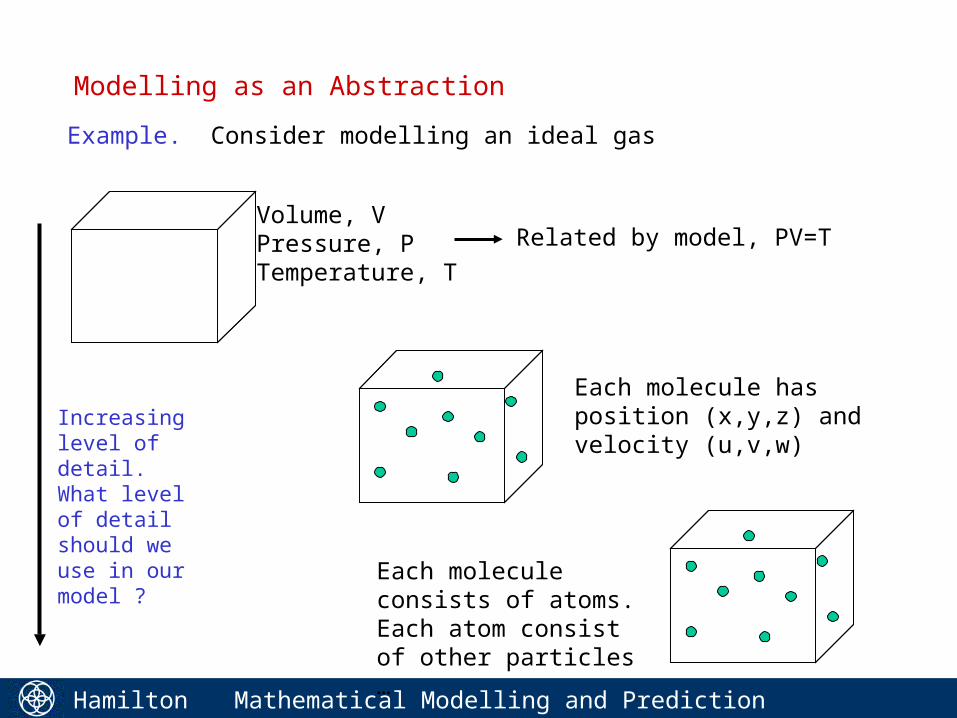
Modelling as an Abstraction
Example. Consider modelling an ideal gas
Volume, VPressure, PTemperature, T
Related by model, PV=T
Each molecule has position (x,y,z) and velocity (u,v,w)
Each molecule consists of atoms. Each atom consist of other particles …
Increasing level of detail. What level of detail should we use in our model ?
Hamilton Institute
Mathematical Modelling and Prediction 4
Selecting the appropriate level of abstraction/detail is a key part of modelling.
Strongly application dependent and something of an “art”. Not dealt with in detail in this course, but we do note that it is linked to what we are able to observe/measure as well as to the purpose for which the model is intended.
- because when assessing a model against the real system we cannot decide between models which generate the same predicted observations
Modelling as an Abstraction
Hamilton Institute
Mathematical Modelling and Prediction 5
Example – A simple population model (the “logistic map”)
Let Ni be the population in year i
A crude model for population growth is that
Ni=aNi-1
When a>1, the population increases (unboundedly) each year. When a<1, the population decreases each year until it reaches zero (extinction).
This is obviously an oversimplification. We need to account for overcrowding and limited resources i.e. we expect the value of parameter a to vary with the population N.
Now have
Ni=a(Ni-1)Ni-1
Lets assume that a(N)= (1-N) for N in the interval [0,1]See www.hamilton.ie/cs416/logisticmap.htm for arguments in support of this choice.
Hamilton Institute
Mathematical Modelling and Prediction 6
Example – A simple population model (the “logistic map”)
Ni= (1-Ni-1)Ni-1 “Logistic Map”
Note that this is a very much simplified model. Are these simplifications justified ? That is, how “good” is this model.
-depends on what we want to use it for.-can compare predictions of model with observed behaviour to validate model/establish accuracy. Availability of observations places fundamental limit on quality of model.
What can we use the model for ?
The structure of the model reflects our understanding of the structure of the system-a model organises our experiences and observations
We can solve the model equations to make predictions- decision support
Hamilton Institute
Mathematical Modelling and Prediction 7
0 0.1 0.2 0.3 0.4 0.5 0.6 0.7 0.8 0.9 10
0.1
0.2
0.3
0.4
0.5
0.6
0.7
0.8
0.9
1
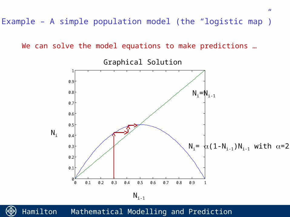
Example – A simple population model (the “logistic map”)
We can solve the model equations to make predictions …
Ni-1
Ni
Ni= (1-Ni-1)Ni-1 with =2
Ni=Ni-1
Graphical Solution
Hamilton Institute
Mathematical Modelling and Prediction 8
With =2, a stationary point exists to which all solutions in interval [0,1] are eventually attracted.
NB: “stationary point” = “equilibrium point” = “steady-state solution”
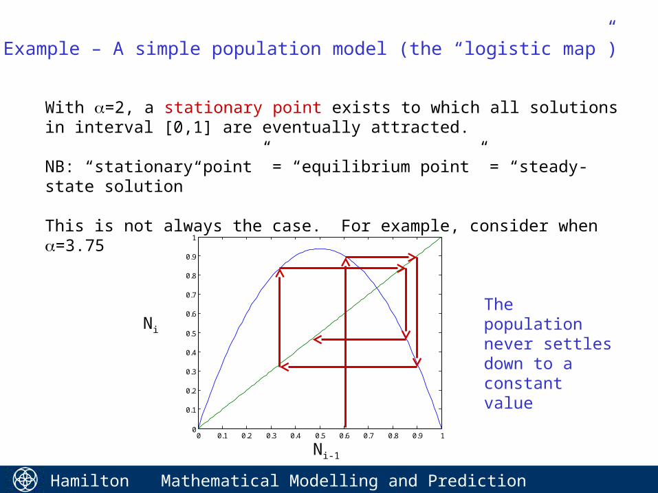
This is not always the case. For example, consider when =3.75
Example – A simple population model (the “logistic map”)
Ni-1
Ni
0 0.1 0.2 0.3 0.4 0.5 0.6 0.7 0.8 0.9 10
0.1
0.2
0.3
0.4
0.5
0.6
0.7
0.8
0.9
1
The population never settles down to a constant value

Hamilton Institute
Mathematical Modelling and Prediction 9
Queue length, q. Service rate, B packets/s.
Packets arrive at times t0,t1,t2,…
Ignoring servicing of packets just now, when a packet arrives we have
q(tn)=min(q(tn-1)+1, qmax)
Now, interval between two packets is tn-tn-1. During this interval B(tn-tn-1) packets are serviced i.e. removed from the queue. The queue size cannot fall below zero. So, we have as our model
Q=min(q(tn-1)+1-B(tn-tn-1) , qmax)q(tn)=max(Q,0)
Example: Server with buffer/queue
Hamilton Institute
Mathematical Modelling and Prediction 10
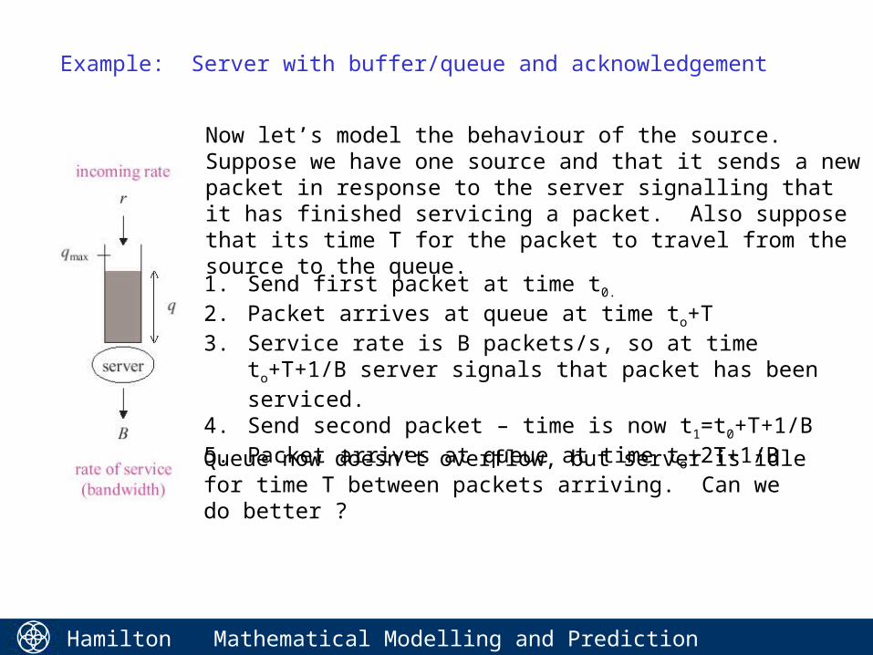
Now let’s model the behaviour of the source. Suppose we have one source and that it sends a new packet in response to the server signalling that it has finished servicing a packet. Also suppose that its time T for the packet to travel from the source to the queue.
Example: Server with buffer/queue and acknowledgement
1. Send first packet at time t0.
2. Packet arrives at queue at time to+T3. Service rate is B packets/s, so at time to+T+1/B
server signals that packet has been serviced.4. Send second packet – time is now t1=t0+T+1/B5. Packet arrives at queue at time to+2T+1/B Queue now doesn’t overflow, but server is idle for time T between packets arriving. Can we do better ?
Hamilton Institute
Mathematical Modelling and Prediction 11
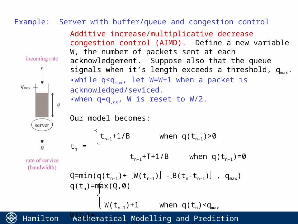
Additive increase/multiplicative decrease congestion control (AIMD). Define a new variable W, the number of packets sent at each acknowledgement. Suppose also that the queue signals when it’s length exceeds a threshold, qmax.
•while q<qmax, let W=W+1 when a packet is acknowledged/seviced.•when q=q,ax, W is reset to W/2.
Our model becomes:
tn-1+1/B when q(tn-1)>0tn = tn-1+T+1/B when q(tn-1)=0
Q=min(q(tn-1)+ W(tn-1) -B(tn-tn-1) , qmax)q(tn)=max(Q,0)
W(tn-1)+1 when q(tn)<qmax
W(tn)= W(tn-1)/2 when q(tn)=qmax
Example: Server with buffer/queue and congestion control
Hamilton Institute
Mathematical Modelling and Prediction 12
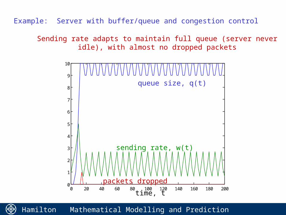
Example: Server with buffer/queue and congestion control
0 20 40 60 80 100 120 140 160 180 2000
1
2
3
4
5
6
7
8
9
10
time, t
queue size, q(t)
sending rate, w(t)
packets dropped
Sending rate adapts to maintain full queue (server never idle), with almost no dropped packets
Hamilton Institute
Mathematical Modelling and Prediction 13
Example: Server with buffer/queue and congestion control
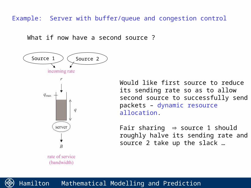
What if now have a second source ?
Source 2Source 1
Would like first source to reduce its sending rate so as to allow second source to successfully send packets – dynamic resource allocation.
Fair sharing source 1 should roughly halve its sending rate and source 2 take up the slack …
Hamilton Institute
Mathematical Modelling and Prediction 14
0 20 40 60 80 100 120 140 160 180 2000
1
2
3
4
5
6
7
8
9
10
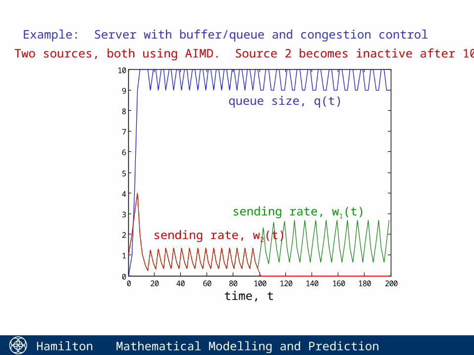
Example: Server with buffer/queue and congestion control
time, t
queue size, q(t)
sending rate, w1(t)
sending rate, w2(t)
Two sources, both using AIMD. Source 2 becomes inactive after 100s.
Hamilton Institute
Mathematical Modelling and Prediction 15
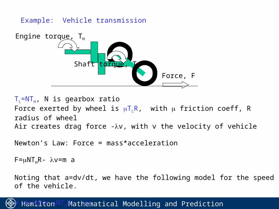
Example: Vehicle transmission
Engine torque, TH
Shaft torque, TL
Force, F
TL=NTH, N is gearbox ratioForce exerted by wheel is TLR, with friction coeff, R radius of wheelAir creates drag force -v, with v the velocity of vehicle
Newton’s Law: Force = mass*acceleration
F=NTHR- v=m a
Noting that a=dv/dt, we have the following model for the speed of the vehicle.
m dv/dt= NTHR - v
Hamilton Institute
Mathematical Modelling and Prediction 16
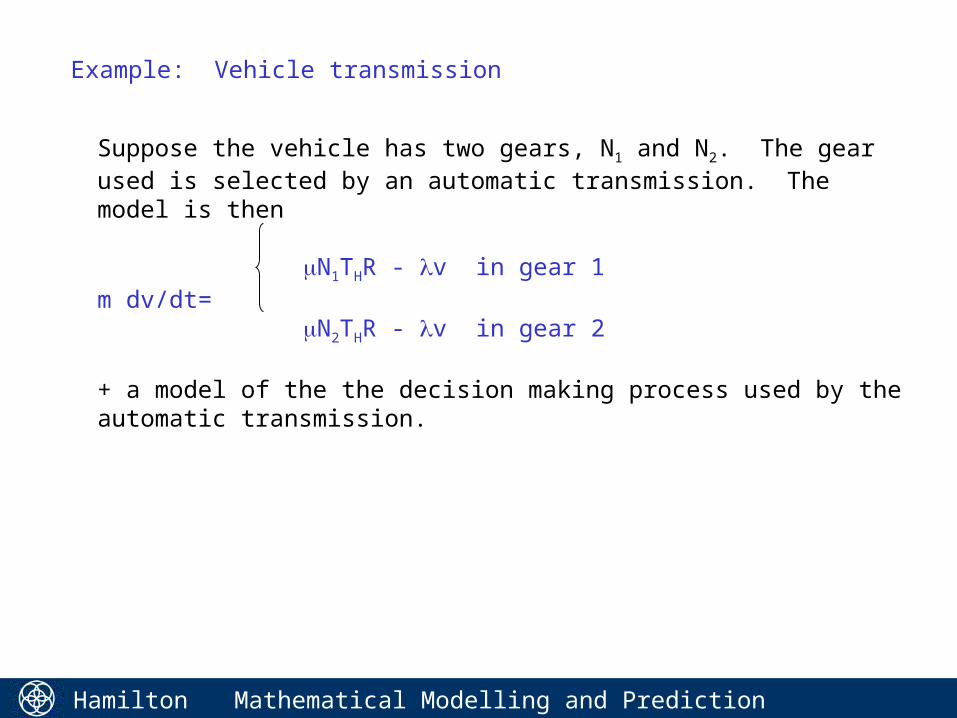
Example: Vehicle transmission
Suppose the vehicle has two gears, N1 and N2. The gear used is selected by an automatic transmission. The model is then
N1THR - v in gear 1m dv/dt=
N2THR - v in gear 2
+ a model of the the decision making process used by the automatic transmission.
Hamilton Institute
Mathematical Modelling and Prediction 17
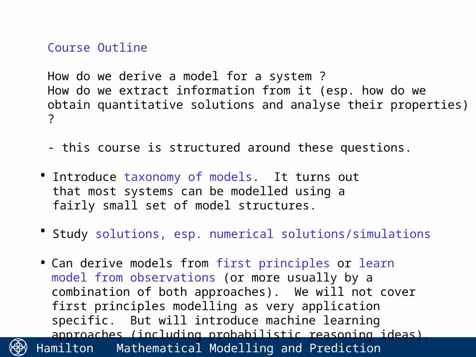
Course Outline
How do we derive a model for a system ?How do we extract information from it (esp. how do we obtain quantitative solutions and analyse their properties) ?
- this course is structured around these questions.
Introduce taxonomy of models. It turns out that most systems can be modelled using a fairly small set of model structures.
•
Study solutions, esp. numerical solutions/simulations•
Can derive models from first principles or learn model from observations (or more usually by a combination of both approaches). We will not cover first principles modelling as very application specific. But will introduce machine learning approaches (including probabilistic reasoning ideas).
•
Hamilton Institute
Mathematical Modelling and Prediction 18
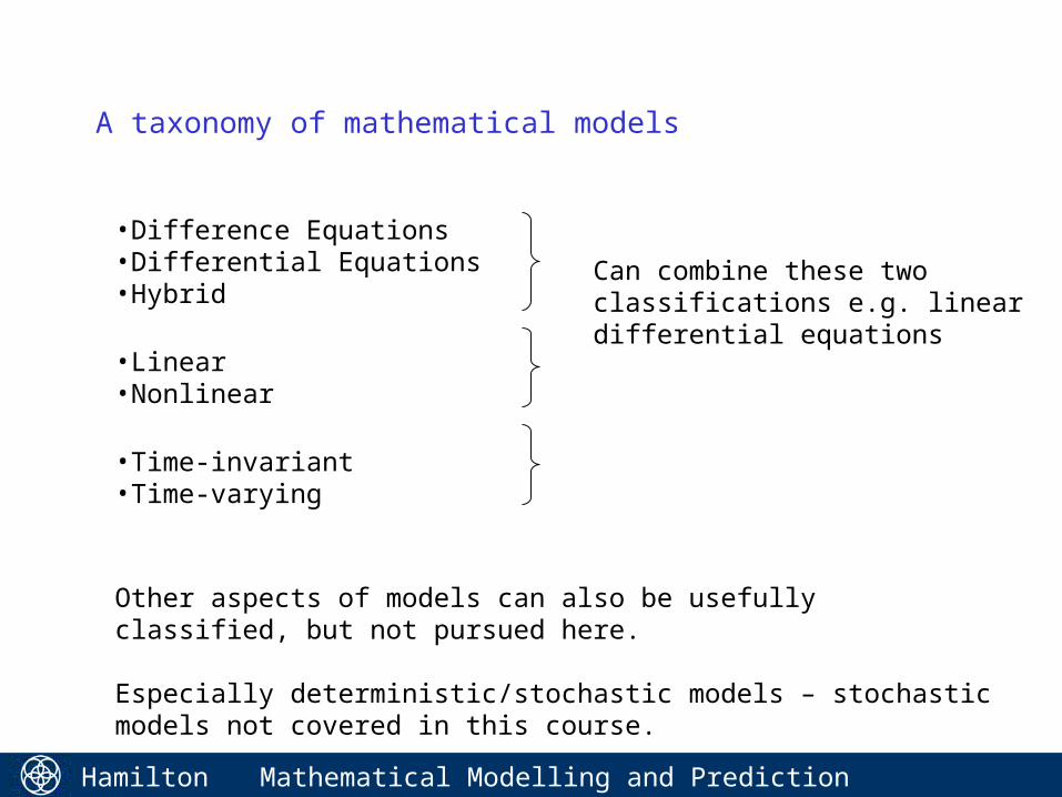
A taxonomy of mathematical models
•Difference Equations•Differential Equations•Hybrid
•Linear•Nonlinear
•Time-invariant•Time-varying
Other aspects of models can also be usefully classified, but not pursued here.
Especially deterministic/stochastic models – stochastic models not covered in this course.
Can combine these two classifications e.g. linear differential equations
Hamilton Institute
Mathematical Modelling and Prediction 19
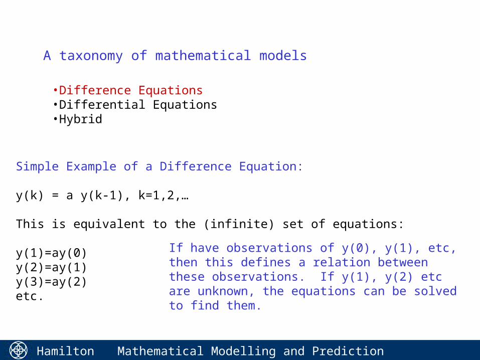
A taxonomy of mathematical models
•Difference Equations•Differential Equations•Hybrid
Simple Example of a Difference Equation:
y(k) = a y(k-1), k=1,2,…
This is equivalent to the (infinite) set of equations:
y(1)=ay(0)y(2)=ay(1)y(3)=ay(2)etc.
If have observations of y(0), y(1), etc, then this defines a relation between these observations. If y(1), y(2) etc are unknown, the equations can be solved to find them.
Hamilton Institute
Mathematical Modelling and Prediction 20
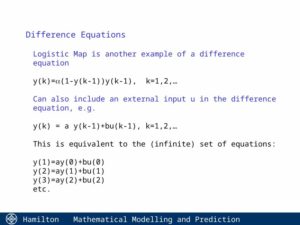
Difference Equations
Logistic Map is another example of a difference equation
y(k)=(1-y(k-1))y(k-1), k=1,2,…
Can also include an external input u in the difference equation, e.g.
y(k) = a y(k-1)+bu(k-1), k=1,2,…
This is equivalent to the (infinite) set of equations:
y(1)=ay(0)+bu(0)y(2)=ay(1)+bu(1)y(3)=ay(2)+bu(2)etc.
Hamilton Institute
Mathematical Modelling and Prediction 21
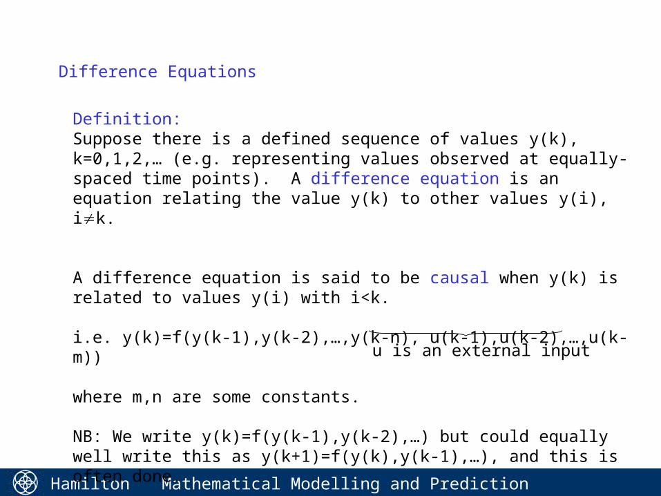
Definition:Suppose there is a defined sequence of values y(k), k=0,1,2,… (e.g. representing values observed at equally-spaced time points). A difference equation is an equation relating the value y(k) to other values y(i), ik.
A difference equation is said to be causal when y(k) is related to values y(i) with i<k.
i.e. y(k)=f(y(k-1),y(k-2),…,y(k-n), u(k-1),u(k-2),…,u(k-m))
where m,n are some constants.
NB: We write y(k)=f(y(k-1),y(k-2),…) but could equally well write this as y(k+1)=f(y(k),y(k-1),…), and this is often done.
Difference Equations
u is an external input
Hamilton Institute
Mathematical Modelling and Prediction 22
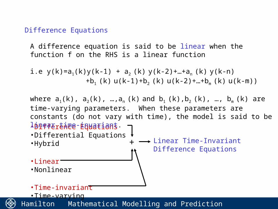
•Difference Equations•Differential Equations•Hybrid
•Linear•Nonlinear
•Time-invariant•Time-varying
Linear Time-Invariant Difference Equations
+
Difference Equations
A difference equation is said to be linear when the function f on the RHS is a linear function
i.e y(k)=a1(k)y(k-1) + a2 (k) y(k-2)+…+an (k) y(k-n)+b1 (k) u(k-1)+b2 (k) u(k-2)+…+bm (k) u(k-m))
where a1(k), a2(k), …,an (k) and b1 (k),b2 (k), …, bm (k) are time-varying parameters. When these parameters are constants (do not vary with time), the model is said to be linear time-invariant.
Hamilton Institute
Mathematical Modelling and Prediction 23
Difference Equations
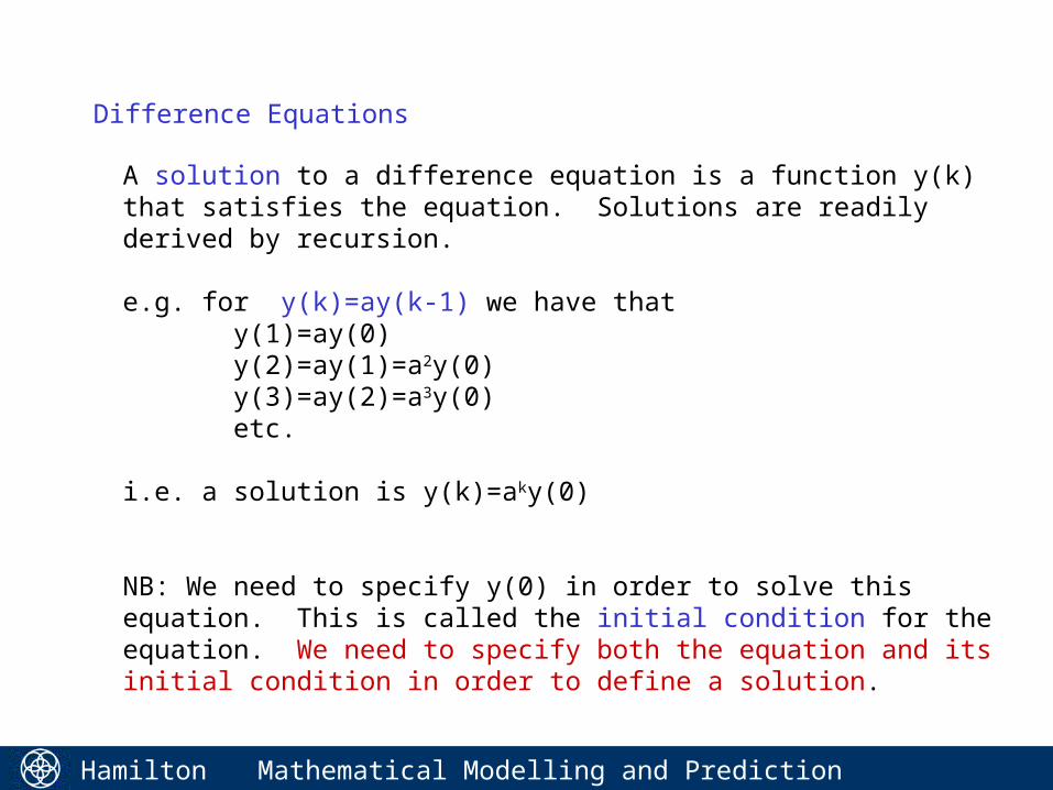
A solution to a difference equation is a function y(k) that satisfies the equation. Solutions are readily derived by recursion.
e.g. for y(k)=ay(k-1) we have that y(1)=ay(0) y(2)=ay(1)=a2y(0) y(3)=ay(2)=a3y(0) etc.
i.e. a solution is y(k)=aky(0)
NB: We need to specify y(0) in order to solve this equation. This is called the initial condition for the equation. We need to specify both the equation and its initial condition in order to define a solution.
Hamilton Institute
Mathematical Modelling and Prediction 24
More generally,
y(k)=f(y(k-1),y(k-2),…,y(k-n), u(k-1),u(k-2),…,u(k-m))
We assume that the input values u(k) are defined beforehand. We must also specify y(0), y(1), …, y(n-1) in order to define a solution – in general the initial condition must specify n values.
Difference Equations – Initial Conditions
Hamilton Institute
Mathematical Modelling and Prediction 25
•Note that a difference equation need not have any solution.
e.g. y(k)2=-(1+y(k-1)2)
has no solution since y(k)2 can never be negative.
•Also, even when a solution exists, it need not be unique i.e. there may exist many solutions.
e.g. sin y(k) = y(k-1)
Generally, however, a model of a physical system can be expected to possess a solution which is unique.
Difference Equations – Existence & Uniqueness of Solutions
Hamilton Institute
Mathematical Modelling and Prediction 26
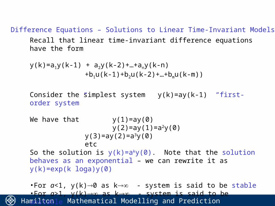
Recall that linear time-invariant difference equations have the form
y(k)=a1y(k-1) + a2y(k-2)+…+any(k-n)+b1u(k-1)+b2u(k-2)+…+bmu(k-m))
Consider the simplest system y(k)=ay(k-1) “first-order system”
We have that y(1)=ay(0) y(2)=ay(1)=a2y(0)
y(3)=ay(2)=a3y(0)etc
So the solution is y(k)=aky(0). Note that the solution behaves as an exponential – we can rewrite it as y(k)=exp(k loga)y(0)
•For a<1, y(k)0 as k - system is said to be stable•For a>1, y(k) as k - system is said to be unstable•For a=1, solution neither grows of decays
- system is said to be critically stable
Difference Equations – Solutions to Linear Time-Invariant Models
Hamilton Institute
Mathematical Modelling and Prediction 27
0 5 10 15 20 25 30 35 400
0.1
0.2
0.3
0.4
0.5
0.6
0.7
0.8
0.9
1
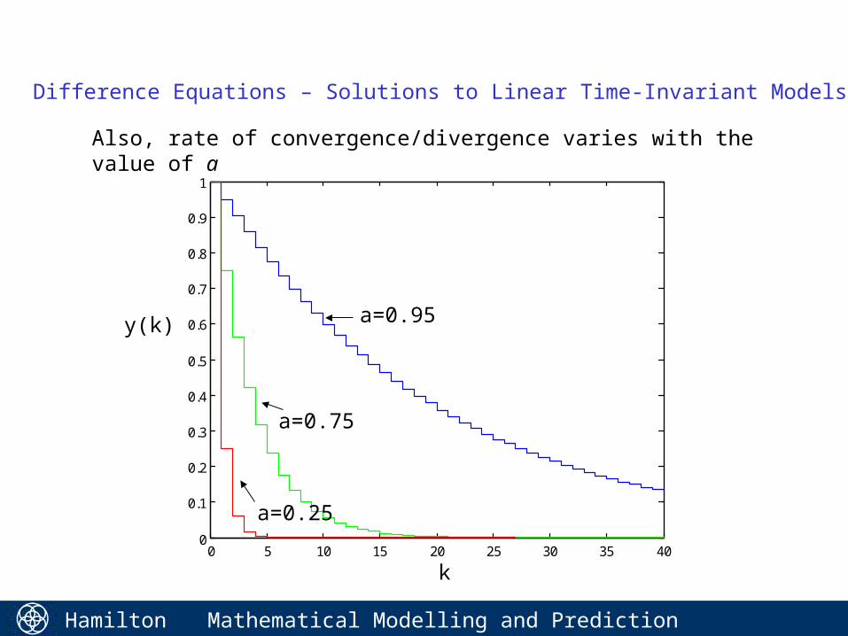
Also, rate of convergence/divergence varies with the value of a
Difference Equations – Solutions to Linear Time-Invariant Models
k
y(k) a=0.95
a=0.75
a=0.25
Hamilton Institute
Mathematical Modelling and Prediction 28
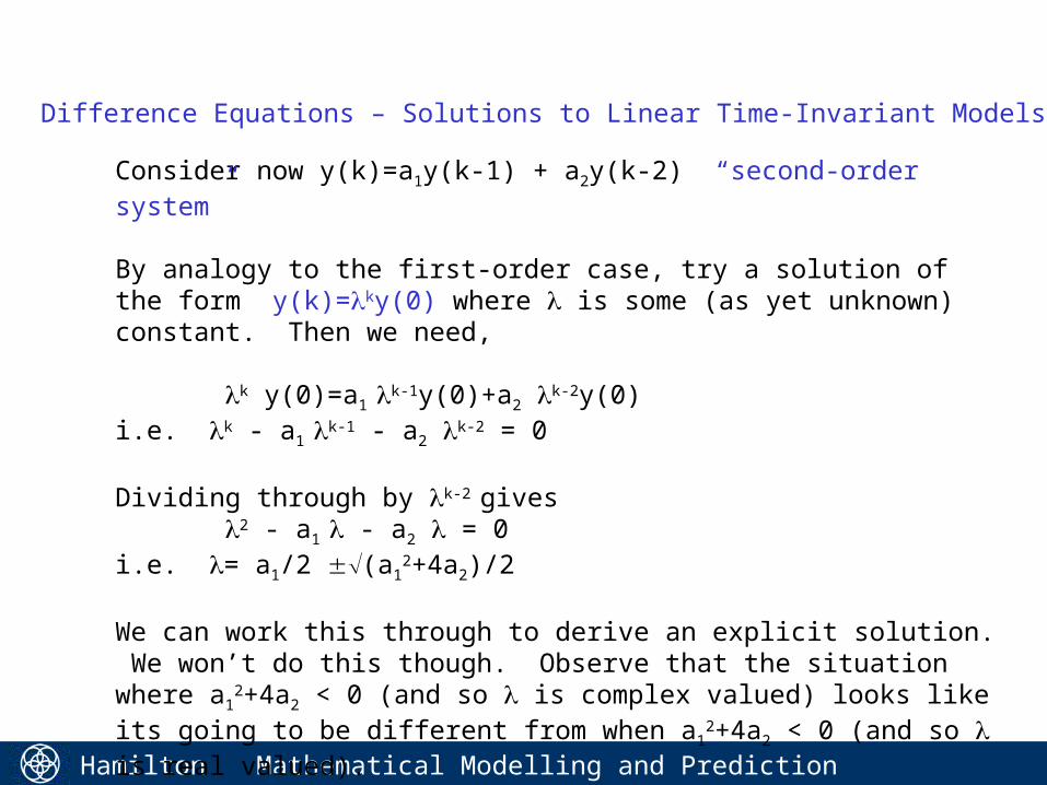
Consider now y(k)=a1y(k-1) + a2y(k-2) “second-order system”
By analogy to the first-order case, try a solution of the form y(k)=ky(0) where is some (as yet unknown) constant. Then we need,
k y(0)=a1 k-1y(0)+a2 k-2y(0)i.e. k - a1 k-1 - a2 k-2 = 0
Dividing through by k-2 gives 2 - a1 - a2 = 0i.e. = a1/2 (a1
2+4a2)/2
We can work this through to derive an explicit solution. We won’t do this though. Observe that the situation where a1
2+4a2 < 0 (and so is complex valued) looks like its going to be different from when a1
2+4a2 < 0 (and so is real valued).
Difference Equations – Solutions to Linear Time-Invariant Models
Hamilton Institute
Mathematical Modelling and Prediction 29
0 2 4 6 8 10 12 14 16 18 20-0.4
-0.2
0
0.2
0.4
0.6
0.8
1
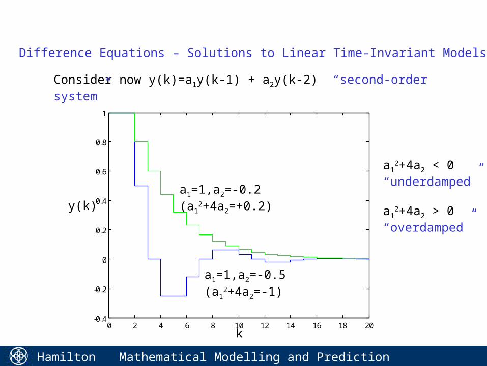
Consider now y(k)=a1y(k-1) + a2y(k-2) “second-order system”
Difference Equations – Solutions to Linear Time-Invariant Models
k
a1=1,a2=-0.5(a1
2+4a2=-1)
a1=1,a2=-0.2(a1
2+4a2=+0.2)y(k)
a12+4a2 < 0
“underdamped”
a12+4a2 > 0
“overdamped”
Hamilton Institute
Mathematical Modelling and Prediction 30
0 20 40 60 80 100 120 140 160 180 200-1
-0.8
-0.6
-0.4
-0.2
0
0.2
0.4
0.6
0.8
1
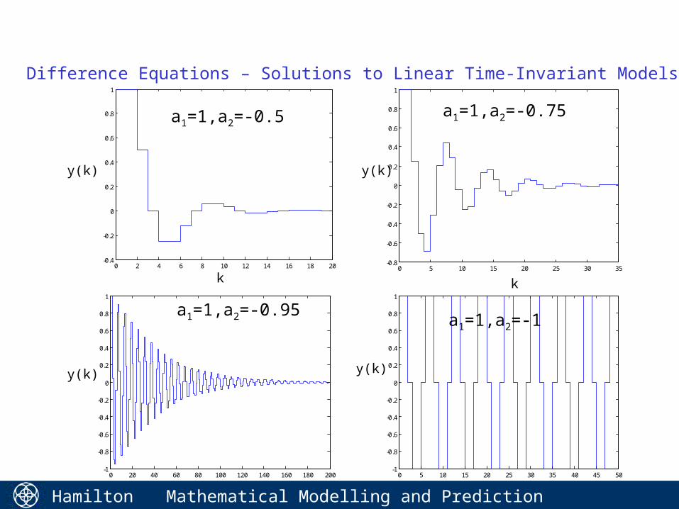
Difference Equations – Solutions to Linear Time-Invariant Models
a1=1,a2=-0.95
0 2 4 6 8 10 12 14 16 18 20-0.4
-0.2
0
0.2
0.4
0.6
0.8
1
a1=1,a2=-0.5
0 5 10 15 20 25 30 35-0.8
-0.6
-0.4
-0.2
0
0.2
0.4
0.6
0.8
1
a1=1,a2=-0.75
0 5 10 15 20 25 30 35 40 45 50-1
-0.8
-0.6
-0.4
-0.2
0
0.2
0.4
0.6
0.8
1
a1=1,a2=-1
k k
y(k)
y(k)
y(k)
y(k)
Hamilton Institute
Mathematical Modelling and Prediction 31
NOTE:
= a1/2 (a12+4a2)/2
Similarly to first-order case,
•For ||<1, y(k)0 as k - system is stable•For ||>1, y(k) as k - system is unstable•For ||=1, solution neither grows of decays
– system is critically stable
When is real valued, system is overdamped (with special case called critically damped when a1
2+4a2=0)-solution to system is the sum of pure exponentials
When is complex valued, system is underdamped-solution to system is oscillatory, with envelope that decays exponentially for stable systems, grows exponentially for unstable systems.
Difference Equations – Solutions to Linear Time-Invariant Models
Hamilton Institute
Mathematical Modelling and Prediction 32
Difference Equations – Equilibria of Linear Time-Invariant Models
For stable systems, the solution converges to a final value as k. This is called the equilibrium point of the system (also called stationary point or steady-state value).
Linear time-invariant difference equation:y(k)=a1y(k-1) + a2y(k-2)+…+any(k-n)
+b1u(k-1)+b2u(k-2)+…+bmu(k-m))
When the input u is zero, at an equilibrium point y we must have: y=a1 y+a2 y+…+an y i.e. y=0
When input is non-zero, the equilibrium point will depend on the input. E.g. say u(k)=u, a constant value. Then
y=a1 y+a2 y+…+an y+b1u+b2u+…+bmu
i.e. y= u (b1+b2+…+bm)/(a1+a2+…+an)
Hamilton Institute
Mathematical Modelling and Prediction 33
Difference Equations – Solutions to Nonlinear Models
For linear difference equations, in qualitative terms only a small number of types of solution can exist (stable, unstable, overdamped, underdamped etc).
For nonlinear difference equations, the situation is much richer.
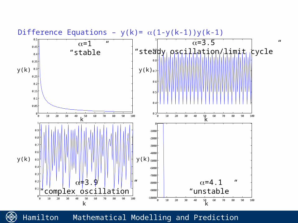
e.g. depending on the value of the parameter , the Logistic Map y(k)= (1-y(k-1))y(k-1) not only has solutions which are stable and unstable but also has steady oscillatory solutions and chaotic solutions (complex oscillations) - these are both types of equilibrium solution which do not have just a single value y.
Hamilton Institute
Mathematical Modelling and Prediction 34
Difference Equations – y(k)= (1-y(k-1))y(k-1)
0 10 20 30 40 50 60 70 80 90 1000
0.05
0.1
0.15
0.2
0.25
0.3
0.35
0.4
0.45
0.5
=1 “stable”
0 10 20 30 40 50 60 70 80 90 1000.3
0.4
0.5
0.6
0.7
0.8
0.9
1
=3.5 “steady oscillation/limit cycle”
0 10 20 30 40 50 60 70 80 90 1000
0.1
0.2
0.3
0.4
0.5
0.6
0.7
0.8
0.9
1
=3.9“complex oscillation”
0 10 20 30 40 50 60 70 80 90 100-10000
-9000
-8000
-7000
-6000
-5000
-4000
-3000
-2000
-1000
0
=4.1“unstable”
k
kk
k
y(k)
y(k)
y(k)
y(k)
Hamilton Institute
Mathematical Modelling and Prediction 35
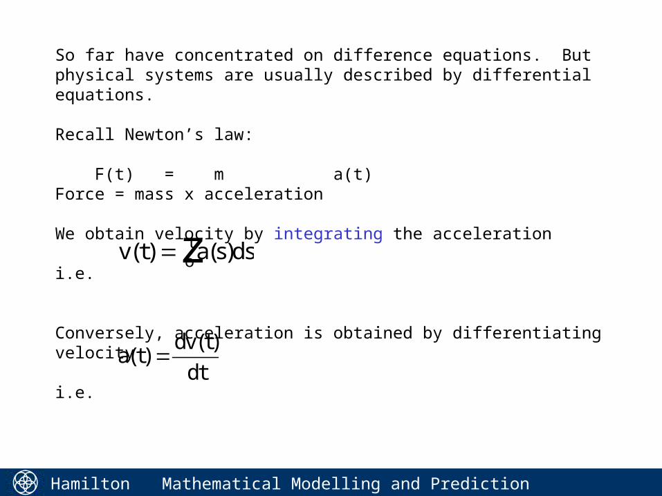
So far have concentrated on difference equations. But physical systems are usually described by differential equations.
Recall Newton’s law:
F(t) = m a(t)Force = mass x acceleration
We obtain velocity by integrating the acceleration i.e.
Conversely, acceleration is obtained by differentiating velocity
i.e.
v t a sot( ) ( )dsz
a tdv t
dt( )
( )
Hamilton Institute
Mathematical Modelling and Prediction 36
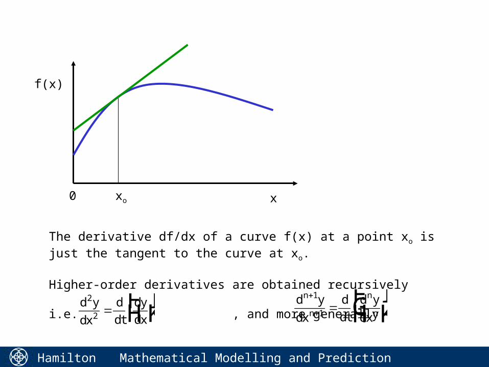
x
f(x)
xo
The derivative df/dx of a curve f(x) at a point xo is just the tangent to the curve at xo.
Higher-order derivatives are obtained recursively
i.e. , and more generally
0
d y
dx
d
dt
dy
dx
2
2 FHIKd y
dx
d
dt
d y
dx
n
n
n
n
FHG
IKJ
1
1
Hamilton Institute
Mathematical Modelling and Prediction 37
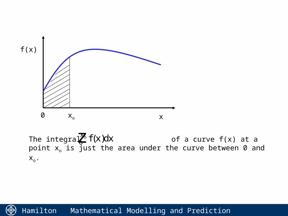
x
f(x)
xo
The integral of a curve f(x) at a point xo is just the area under the curve between 0 and xo.
0
f xoxo ( )dxz
Hamilton Institute
Mathematical Modelling and Prediction 38
Differential Equations
A simple example is
dy(t)/dt = ay(t)
Verify that the solution to this differential equation is:
y(t)=exp(at) y(0)
-compare with the first-order difference equation y(k)=ay(k-1)which has solution y(k)=aky(0)=exp(k log(a)) y(0).
Hamilton Institute
Mathematical Modelling and Prediction 39
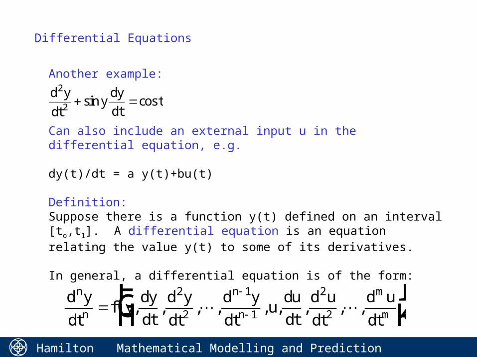
Another example:
Can also include an external input u in the differential equation, e.g.
dy(t)/dt = a y(t)+bu(t)
Definition:Suppose there is a function y(t) defined on an interval [to,t1]. A differential equation is an equation relating the value y(t) to some of its derivatives.
In general, a differential equation is of the form:
Differential Equations
d y
dty
dy
dtt
2
2 sin cos
d y
dtf y
dy
dt
d y
dt
d y
dtu
du
dt
d u
dt
d u
dt
n
n
n
n
m
mFHG
IKJ
, , , , , , , , ,2
2
1
1
2
2
Hamilton Institute
Mathematical Modelling and Prediction 40
Differential Equations
•Difference Equations•Differential Equations•Hybrid
•Linear•Nonlinear
•Time-invariant•Time-varying
Linear Time-Invariant Differential Equations+
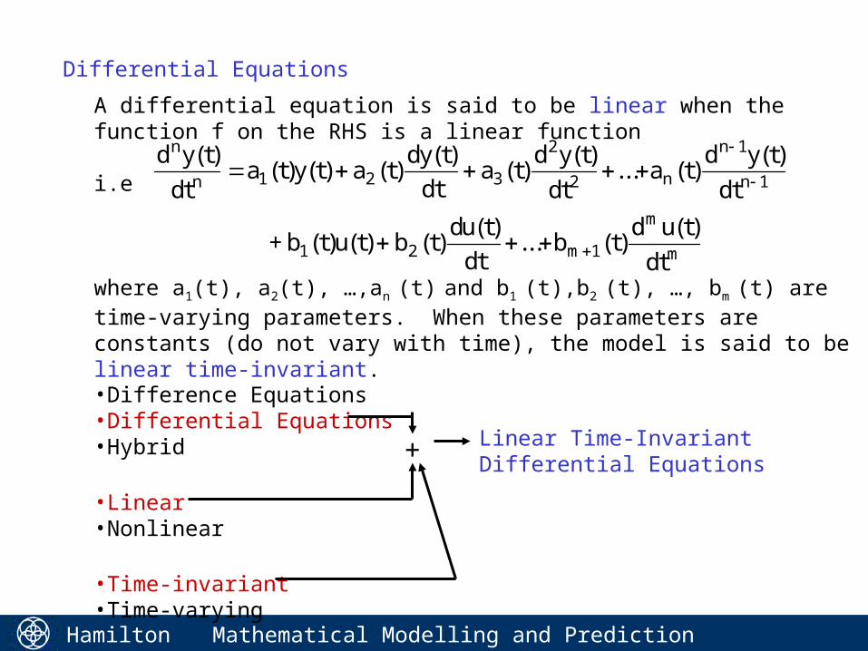
A differential equation is said to be linear when the function f on the RHS is a linear function
i.e
where a1(t), a2(t), …,an (t) and b1 (t),b2 (t), …, bm (t) are time-varying parameters. When these parameters are constants (do not vary with time), the model is said to be linear time-invariant.
d y t
dta t y t a t
dy t
dta t
d y t
dta t
d y t
dt
t u t b tdu t
dtb t
d u t
dt
n
n n
n
n
m
m
m
( )( ) ( ) ( )
( )( )
( )... ( )
( )
( ) ( ) ( )( )
... ( )( )
1 2 3
2
2
1
1
2 1 + b1
Hamilton Institute
Mathematical Modelling and Prediction 41
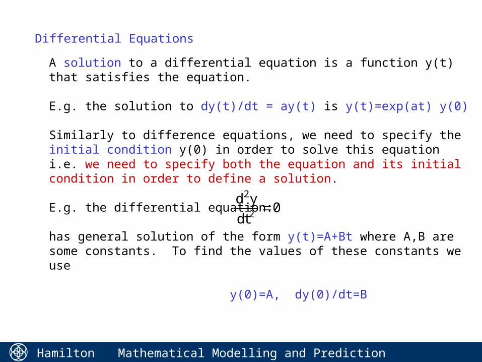
A solution to a differential equation is a function y(t) that satisfies the equation.
E.g. the solution to dy(t)/dt = ay(t) is y(t)=exp(at) y(0)
Similarly to difference equations, we need to specify the initial condition y(0) in order to solve this equation i.e. we need to specify both the equation and its initial condition in order to define a solution.
E.g. the differential equation:
has general solution of the form y(t)=A+Bt where A,B are some constants. To find the values of these constants we use
y(0)=A, dy(0)/dt=B
Differential Equations
d y
dt
2
2 0
Hamilton Institute
Mathematical Modelling and Prediction 42
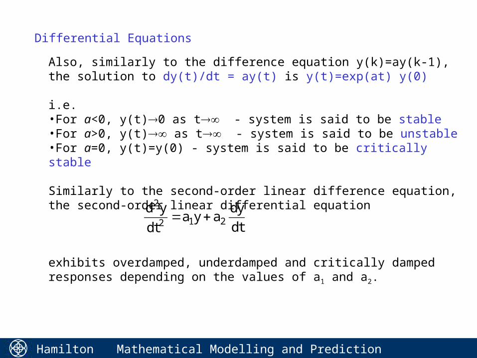
Also, similarly to the difference equation y(k)=ay(k-1), the solution to dy(t)/dt = ay(t) is y(t)=exp(at) y(0)
i.e.•For a<0, y(t)0 as t - system is said to be stable•For a>0, y(t) as t - system is said to be unstable•For a=0, y(t)=y(0) - system is said to be critically stable
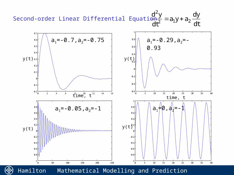
Similarly to the second-order linear difference equation, the second-order linear differential equation
exhibits overdamped, underdamped and critically damped responses depending on the values of a1 and a2.
Differential Equations
d y
dta y a
dy
dt
2
2 1 2
Hamilton Institute
Mathematical Modelling and Prediction 43
0 2 4 6 8 10 12 14 16-0.2
-0.1
0
0.1
0.2
0.3
0.4
0.5
0.6
0.7
0 5 10 15 20 25 30 35 40-1
-0.8
-0.6
-0.4
-0.2
0
0.2
0.4
0.6
0.8
1
a1=0,a2=-1
0 5 10 15 20 25 30 35 40-0.6
-0.4
-0.2
0
0.2
0.4
0.6
0.8
1
0 50 100 150 200 250-1
-0.8
-0.6
-0.4
-0.2
0
0.2
0.4
0.6
0.8
1
Second-order Linear Differential Equation
a1=-0.05,a2=-1
a1=-0.7,a2=-0.75 a1=-0.29,a2=-0.93
time, t time, t
y(t)
y(t)
y(t)
y(t)
d y
dta y a
dy
dt
2
2 1 2
Hamilton Institute
Mathematical Modelling and Prediction 44
0 20 40 60 80 100 120 140 160 180 200-1
-0.8
-0.6
-0.4
-0.2
0
0.2
0.4
0.6
0.8
1
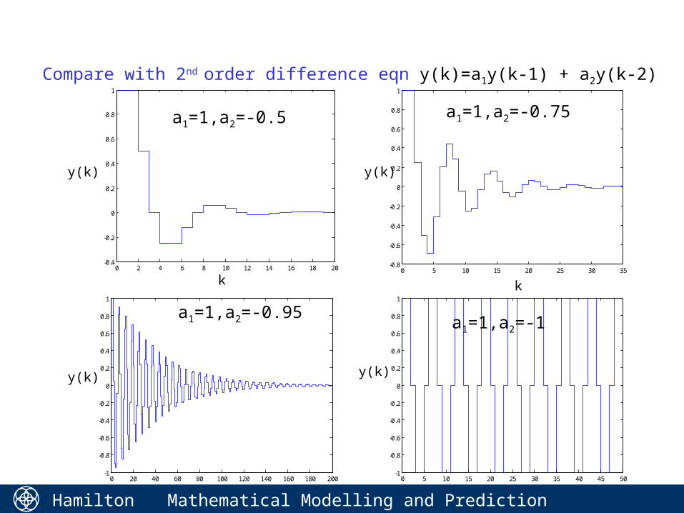
Compare with 2nd order difference eqn y(k)=a1y(k-1) + a2y(k-2)
a1=1,a2=-0.95
0 2 4 6 8 10 12 14 16 18 20-0.4
-0.2
0
0.2
0.4
0.6
0.8
1
a1=1,a2=-0.5
0 5 10 15 20 25 30 35-0.8
-0.6
-0.4
-0.2
0
0.2
0.4
0.6
0.8
1
a1=1,a2=-0.75
0 5 10 15 20 25 30 35 40 45 50-1
-0.8
-0.6
-0.4
-0.2
0
0.2
0.4
0.6
0.8
1
a1=1,a2=-1
k k
y(k)
y(k)
y(k)
y(k)
Hamilton Institute
Mathematical Modelling and Prediction 45
Linear difference and differential equations are closely related.
NOTE: This is generally only true for linear equations. Nonlinear equations seem to be fundamentally different,e.g. chaos can exist in first-order difference equations (such as the logistic map), but not in first-order differential equations (we need to go to at least third order to find a differential equation which exhibits chaos).
Recall definition of derivative:
This suggests that a derivative might be approximated by the finite difference:
for small h. This is called the Euler approximation. We expect that as h is made smaller, the accuracy of the approximation improves.
dy t
dt
y t h y t
hh
( )lim
( ) ( )
0
dy t
dt
y t h y t
h
( ) ( ) ( )
Hamilton Institute
Mathematical Modelling and Prediction 46
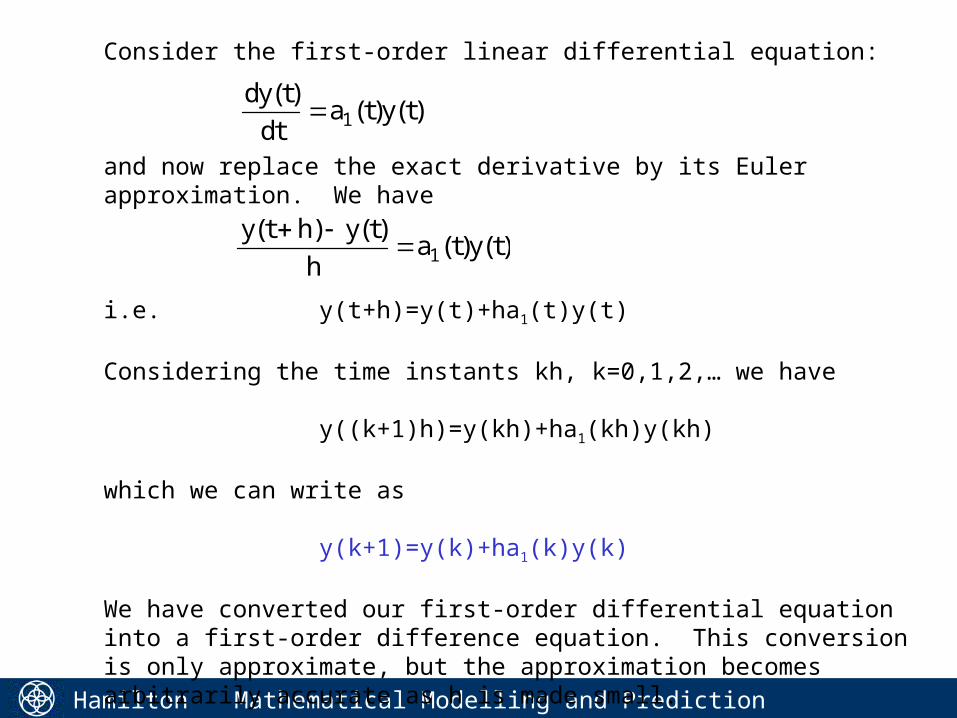
Consider the first-order linear differential equation:
and now replace the exact derivative by its Euler approximation. We have
i.e. y(t+h)=y(t)+ha1(t)y(t)
Considering the time instants kh, k=0,1,2,… we have
y((k+1)h)=y(kh)+ha1(kh)y(kh)
which we can write as
y(k+1)=y(k)+ha1(k)y(k)
We have converted our first-order differential equation into a first-order difference equation. This conversion is only approximate, but the approximation becomes arbitrarily accurate as h is made small.
dy t
dta t y t
( )( ) ( ) 1
y t h y t
ha t y t
( ) ( )( ) ( )
1
Hamilton Institute
Mathematical Modelling and Prediction 47
Impulse Response
Time (sec)
Am
plitu
de
0 5 10 15 20 25-0.2
-0.1
0
0.1
0.2
0.3
0.4
0.5
0.6
0.7
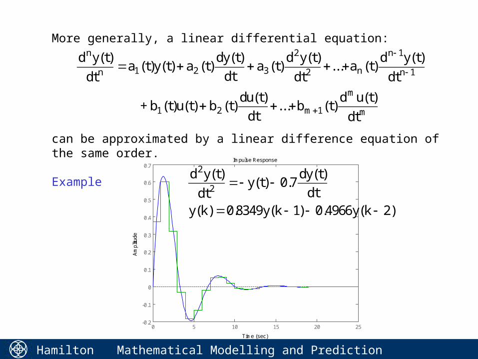
More generally, a linear differential equation:
can be approximated by a linear difference equation of the same order.
Example
d y t
dta t y t a t
dy t
dta t
d y t
dta t
d y t
dt
t u t b tdu t
dtb t
d u t
dt
n
n n
n
n
m
m
m
( )( ) ( ) ( )
( )( )
( )... ( )
( )
( ) ( ) ( )( )
... ( )( )
1 2 3
2
2
1
1
2 1 + b1
d y t
dty t
dy t
dty k y k y k
2
2 0 7
0 8349 1 0 2
( )( ) .
( )
( ) . ( ) .4966 ( )
Hamilton Institute
Mathematical Modelling and Prediction 48
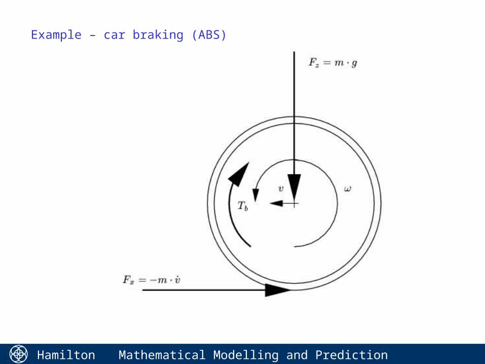
Example – car braking (ABS)
Hamilton Institute
Mathematical Modelling and Prediction 49
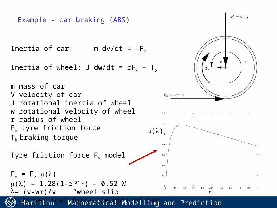
Example – car braking (ABS)
Inertia of car: m dv/dt = -Fx
Inertia of wheel: J dw/dt = rFx – Tb
m mass of carV velocity of carJ rotational inertia of wheelw rotational velocity of wheelr radius of wheelFx tyre friction forceTb braking torque
Tyre friction force Fx model
Fx = Fz ()() = 1.28(1-e-24 ) – 0.52 = (v-wr)/v “wheel slip”Fz is vertical force (weight) of car
0 0.1 0.2 0.3 0.4 0.5 0.6 0.7 0.8 0.9 10
0.2
0.4
0.6
0.8
1
1.2
1.4
()
Hamilton Institute
Mathematical Modelling and Prediction 50
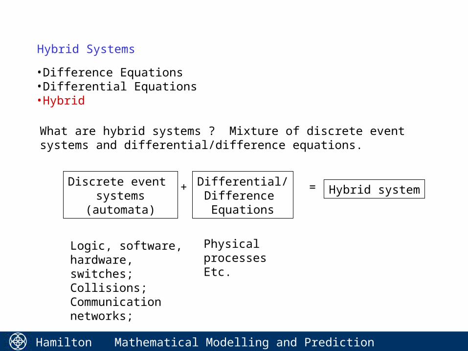
Hybrid Systems
What are hybrid systems ? Mixture of discrete event systems and differential/difference equations.
+ =
•Difference Equations•Differential Equations•Hybrid
Discrete event systems
(automata)
Differential/Difference Equations
Hybrid system
Logic, software, hardware, switches;Collisions;Communication networks;
Physical processesEtc.
Hamilton Institute
Mathematical Modelling and Prediction 51
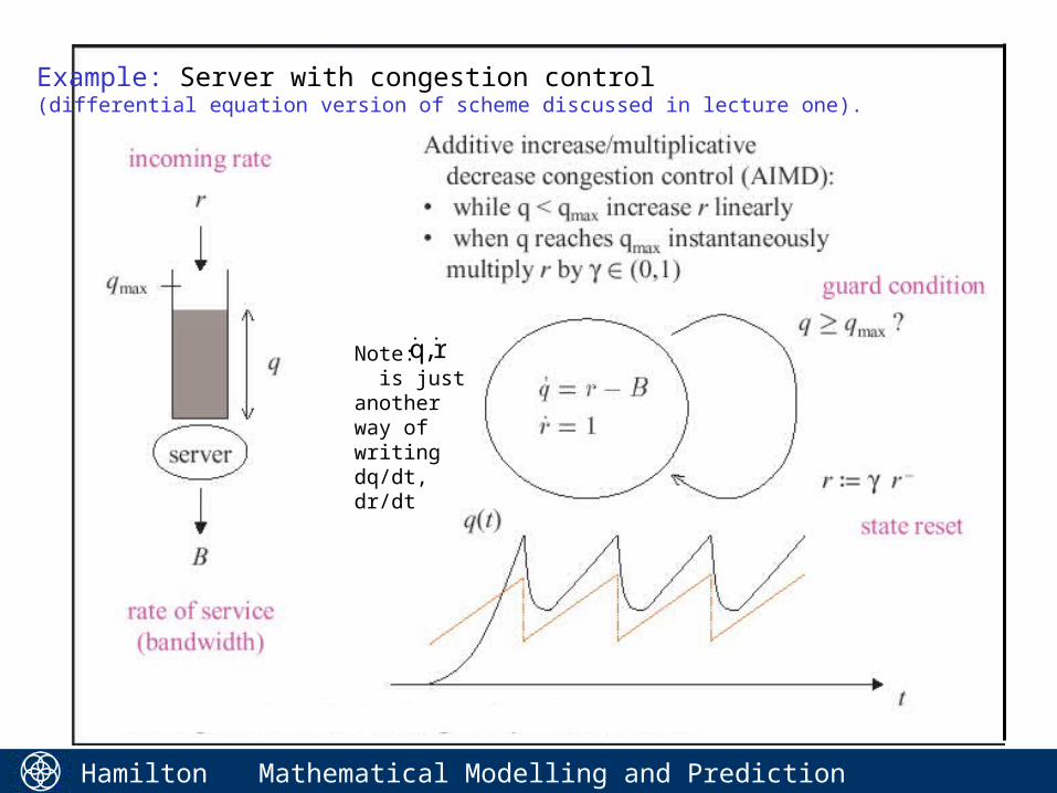
Example: Server with congestion control(differential equation version of scheme discussed in lecture one).
, q rNote: is just another way of writing dq/dt, dr/dt
Hamilton Institute
Mathematical Modelling and Prediction 52
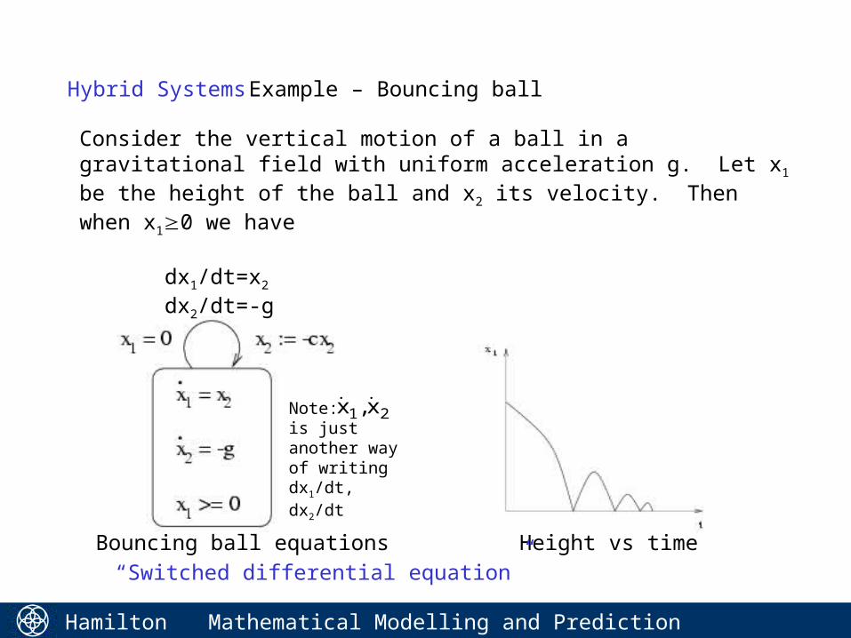
Hybrid Systems Example – Bouncing ball
Bouncing ball equations Height vs time
Consider the vertical motion of a ball in a gravitational field with uniform acceleration g. Let x1 be the height of the ball and x2 its velocity. Then when x10 we have
dx1/dt=x2
dx2/dt=-g
“Switched differential equation”
, x x1 2Note: is just another way of writing dx1/dt, dx2/dt
Hamilton Institute
Mathematical Modelling and Prediction 53
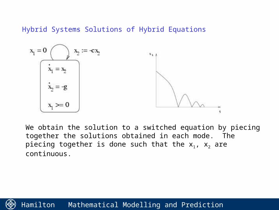
Hybrid Systems - Solutions of Hybrid Equations
We obtain the solution to a switched equation by piecing together the solutions obtained in each mode. The piecing together is done such that the x1, x2 are continuous.
Hamilton Institute
Mathematical Modelling and Prediction 54
Hybrid Systems
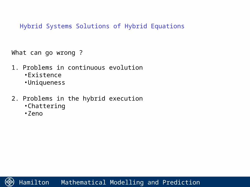
What can go wrong ?
1. Problems in continuous evolution•Existence•Uniqueness
2. Problems in the hybrid execution•Chattering•Zeno
- Solutions of Hybrid Equations
Hamilton Institute
Mathematical Modelling and Prediction 55
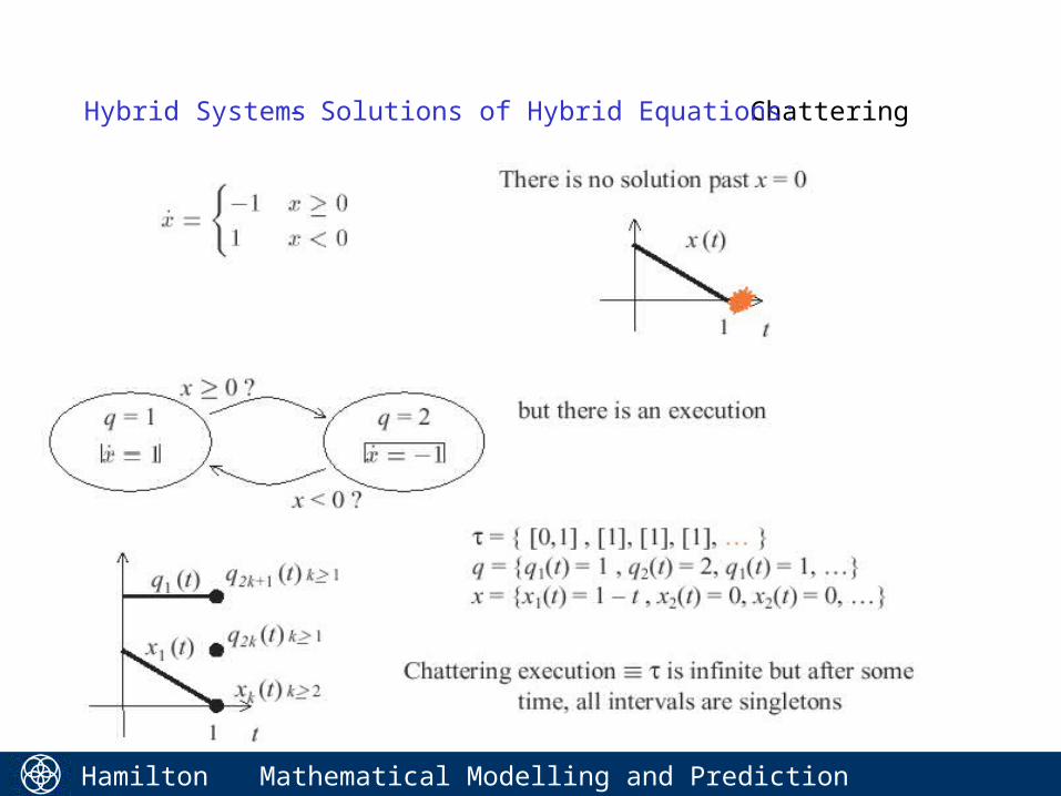
Hybrid Systems Chattering - Solutions of Hybrid Equations:
Hamilton Institute
Mathematical Modelling and Prediction 56
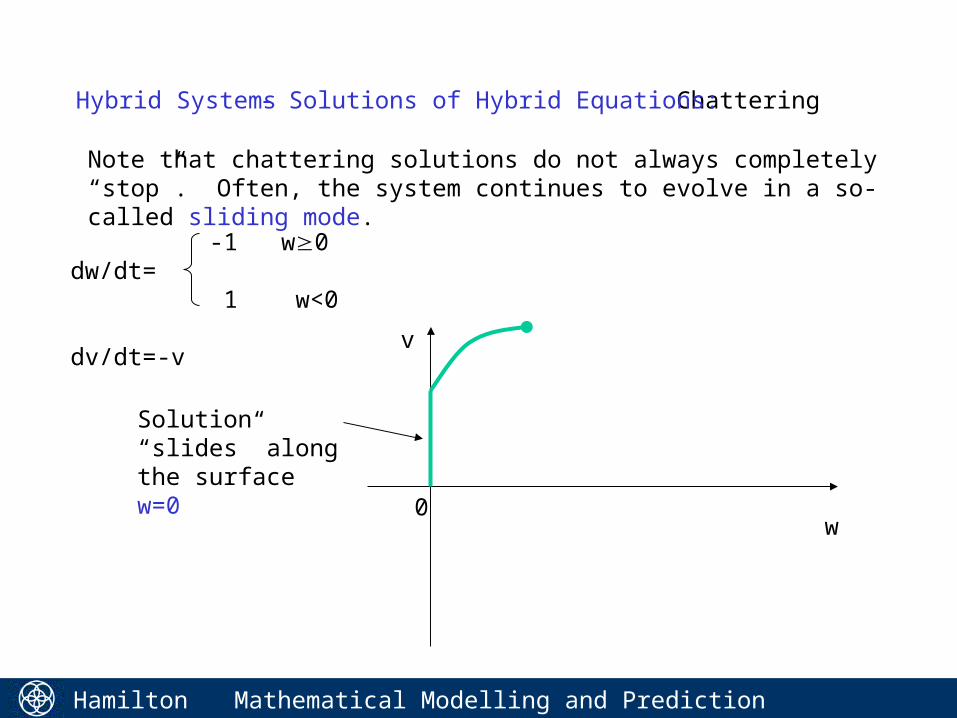
Hybrid Systems
-1 w0dw/dt=
1 w<0
dv/dt=-v
Note that chattering solutions do not always completely “stop”. Often, the system continues to evolve in a so-called sliding mode.
w
v
0
Solution “slides” along the surface w=0
Chattering - Solutions of Hybrid Equations:
Hamilton Institute
Mathematical Modelling and Prediction 57
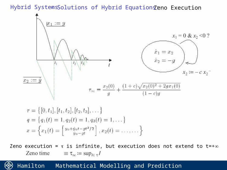
Hybrid Systems
Zeno execution = is infinite, but execution does not extend to t=+
Zeno Execution- Solutions of Hybrid Equations:Hybrid Systems
Hamilton Institute
Mathematical Modelling and Prediction 58
Hybrid Systems - Solutions of Hybrid Equations:
Similarly to difference and differential equations, hybrid systems can be classified as being stable, unstable etc.
Various definitions of stability are used, but all involve the solution decaying to an equilibrium solution as time .
The presence of switching in hybrid systems can sometimes lead to unexpected behaviour….
Hamilton Institute
Mathematical Modelling and Prediction 59
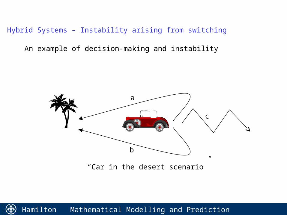
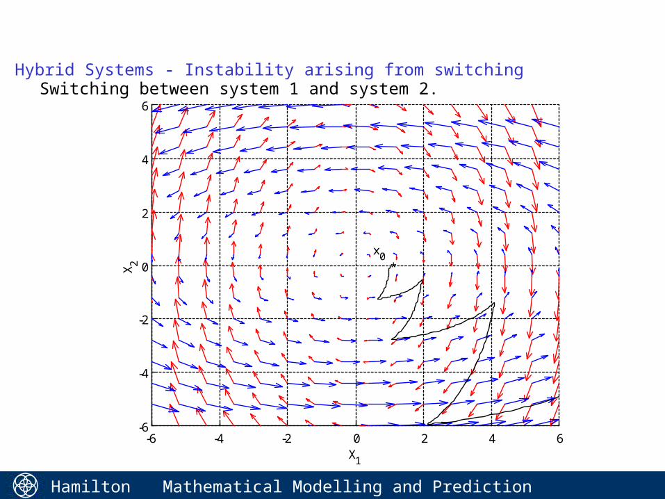
Hybrid Systems – Instability arising from switching
An example of decision-making and instability
“Car in the desert scenario”
a
b
c
Hamilton Institute
Mathematical Modelling and Prediction 60
-6 -4 -2 0 2 4 6-6
-4
-2
0
2
4
6
X1
X 2
Phase plane for A1+b
1c
1T
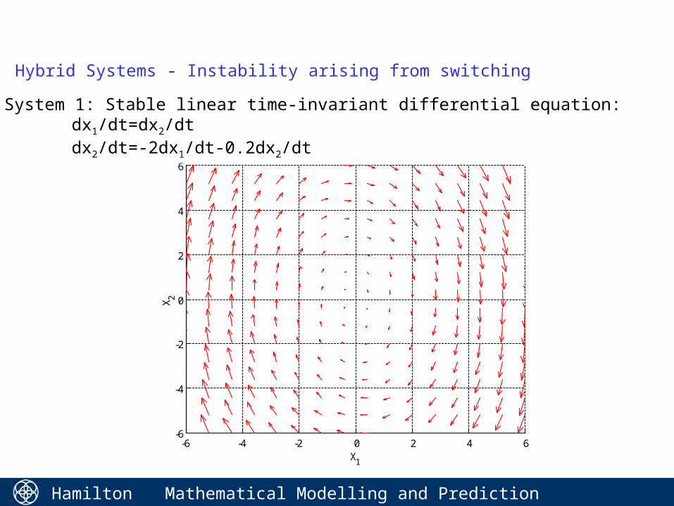
Hybrid Systems - Instability arising from switching
System 1: Stable linear time-invariant differential equation:dx1/dt=dx2/dtdx2/dt=-2dx1/dt-0.2dx2/dt
Hamilton Institute
Mathematical Modelling and Prediction 61
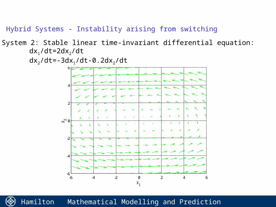
Hybrid Systems - Instability arising from switching
-6 -4 -2 0 2 4 6-6
-4
-2
0
2
4
6
X1
X 2Phase plane for A
2+b
2c
2T
System 2: Stable linear time-invariant differential equation:dx1/dt=2dx2/dtdx2/dt=-3dx1/dt-0.2dx2/dt
Hamilton Institute
Mathematical Modelling and Prediction 62
-6 -4 -2 0 2 4 6-6
-4
-2
0
2
4
6
X1
X 2
*x
0
Hybrid Systems - Instability arising from switchingSwitching between system 1 and system 2.
Hamilton Institute
Mathematical Modelling and Prediction 63
Course Outline
Introduce taxonomy of models. It turns out that most systems can be modelled using a fairly small set of model structures.
•
Study solutions, esp. numerical solutions/simulations•
Can derive models from first principles or learn model from observations (or more usually by a combination of both approaches). We will not cover first principles modelling as very application specific. But will introduce machine learning approaches (including probabilistic reasoning ideas).
•