Mathematical Model of Accumulation of Damaged Proteins and its Impact on Ageing

Dissertation

zur Erlangung des Doktorgrades der Naturwissenschaften

eingereicht am

Fachbereichs Mathematik und Informatik der Freien Universität Berlin

Vorgelegt von Marija Cvijovic

Datum und Ort der mündlichen Prüfung: 30. Januar 2009 in Berlin Gutachter: Prof. Dr. Edda Klipp Prof. Dr. Alexander Bockmayr Prof. Dr. Per Sunnerhagen

2

3

Brain is like a parachute. It works best when it is open.

Frank Zappa

4

5

Abstract Unlike most microorganisms or cell types, the yeast Saccharomyces cerevisiae undergoes

asymmetrical cytokinesis, resulting in a large mother cell and a smaller daughter cell. The

mother cells are characterized by a limited replicative potential accompanied by a

progressive decline in functional capacities, including an increased generation time.

Accumulation of oxidized proteins, a hallmark of ageing, has been shown to occur also

during mother cell-specific ageing, starting during the first G1 phase of newborn cells. It

has been shown that such oxidatively damaged proteins are inherited asymmetrically

during yeast cytokinesis such that most damage is retained in the mother cell.

To investigate the potential benefits of asymmetrical cytokines, we created a

mathematical model to simulate the robustness and fitness of dividing systems displaying

different degrees of damage segregation and size asymmetries.

The model suggests that systems dividing asymmetrically (size-wise) or displaying

damage segregation are more robust than fully symmetrical systems, i.e. can withstand

higher degrees of damage before entering clonal senescence. Both size and damage

asymmetries resulted in a separation of the population into a rejuvenating and an aging

lineage. When considering population fitness, a system producing different-sized

progeny, like budding yeast, is predicted to benefit from damage retention only at high

damage propagation rates. In contrast, the fitness of a system of equal-sized progeny is

enhanced by damage segregation regardless of damage propagation rates suggesting that

damage partitioning may provide an evolutionary advantage also in systems dividing by

binary fission. Using S. pombe as a model, we demonstrate experimentally that damaged,

oxidized, proteins are unevenly partitioned during cytokinesis and that the damage-

enriched sibling suffers from a prolonged generation time and an accelerated aging.

We demonstrate that the damage-enriched cell exhibits a reduced fitness and a shorter

replicative life span. The model confirms the findings in budding yeast and moreover

simulations suggest that asymmetrical distribution of damage increases the fitness of the

cell population as a whole at both low and high damage propagation rates and pushes the

upper limits for how much damage the system can endure before entering clonal

6

senescence. Thus, we suggest that “sibling-specific” aging in unicellular systems may

have evolved as a byproduct of the strong selection for damage segregation during

cytokinesis, and may be more common than previously anticipated.

7

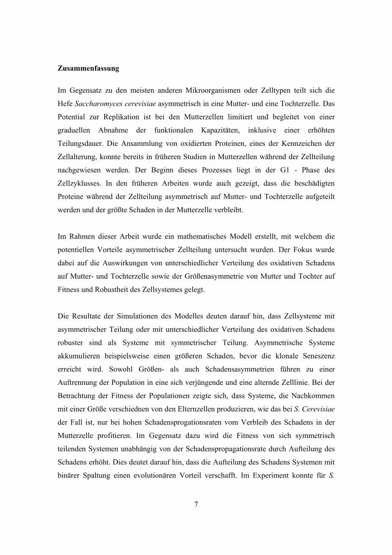
Zusammenfassung

Im Gegensatz zu den meisten anderen Mikroorganismen oder Zelltypen teilt sich die

Hefe Saccharomyces cerevisiae asymmetrisch in eine Mutter- und eine Tochterzelle. Das

Potential zur Replikation ist bei den Mutterzellen limitiert und begleitet von einer

graduellen Abnahme der funktionalen Kapazitäten, inklusive einer erhöhten

Teilungsdauer. Die Ansammlung von oxidierten Proteinen, eines der Kennzeichen der

Zellalterung, konnte bereits in früheren Studien in Mutterzellen während der Zellteilung

nachgewiesen werden. Der Beginn dieses Prozesses liegt in der G1 - Phase des

Zellzyklusses. In den früheren Arbeiten wurde auch gezeigt, dass die beschädigten

Proteine während der Zellteilung asymmetrisch auf Mutter- und Tochterzelle aufgeteilt

werden und der größte Schaden in der Mutterzelle verbleibt.

Im Rahmen dieser Arbeit wurde ein mathematisches Modell erstellt, mit welchem die

potentiellen Vorteile asymmetrischer Zellteilung untersucht wurden. Der Fokus wurde

dabei auf die Auswirkungen von unterschiedlicher Verteilung des oxidativen Schadens

auf Mutter- und Tochterzelle sowie der Größenasymmetrie von Mutter und Tochter auf

Fitness und Robustheit des Zellsystemes gelegt.

Die Resultate der Simulationen des Modelles deuten darauf hin, dass Zellsysteme mit

asymmetrischer Teilung oder mit unterschiedlicher Verteilung des oxidativen Schadens

robuster sind als Systeme mit symmetrischer Teilung. Asymmetrische Systeme

akkumulieren beispielsweise einen größeren Schaden, bevor die klonale Seneszenz

erreicht wird. Sowohl Größen- als auch Schadensasymmetrien führen zu einer

Auftrennung der Population in eine sich verjüngende und eine alternde Zelllinie. Bei der

Betrachtung der Fitness der Populationen zeigte sich, dass Systeme, die Nachkommen

mit einer Größe verschiednen von den Elternzellen produzieren, wie das bei S. Cerevisiae

der Fall ist, nur bei hohen Schadensprogationsraten vom Verbleib des Schadens in der

Mutterzelle profitieren. Im Gegensatz dazu wird die Fitness von sich symmetrisch

teilenden Systemen unabhängig von der Schadenspropagationsrate durch Aufteilung des

Schadens erhöht. Dies deutet darauf hin, dass die Aufteilung des Schadens Systemen mit

binärer Spaltung einen evolutionären Vorteil verschafft. Im Experiment konnte für S.

8

Pombe als Modelorganismus für ein solches System gezeigt werden, dass der oxidative

Schaden während der Zellteilung in unterschiedlicher Höhe auf die Geschwisterzellen

aufgeteilt werden. Die Zelle, bei der der höhere Schaden verbleibt, teilt sich in der Folge

langsamer und altert schneller.

Es konnte ebenfalls gezeigt werden, dass die Fitness sowie die replikative Lebensspanne

in Zellen mit höheren oxidativen Schäden reduziert ist. Das Model bestätigt die

experimentellen Resultate für S. Cerevisiae und legt außerdem nahe, dass die

asymmetrische Verteilung des Schadens die Fitness einer Zellpopulation sowohl für hohe

als auch für niedrige Schadenspropagationsraten erhöht. Darüber hinaus wird dadurch die

obere Schranke für den Schaden, ab welcher klonale Seneszenz erfolgt, weiter nach oben

verlagert. Dies bedeutet, dass das geschwisterspezifische Altern als evolutionäres

Nebenprodukt aus dem Selektionsvorteil für Systeme mit asymmetrischer

Schadensaufteilung entstanden ist und möglicherweise weiter verbreitet ist, als bislang

angenommen wurde.

9

Table of Contents 1. Systems Biology....................................................................................................... 15

1.1 Modeling Biological Systems ................................................................................. 16 1.1.1 Boolean Networks............................................................................................ 16 1.2.1 Stochastic Modeling......................................................................................... 17

1.2 ODE models............................................................................................................ 18 1.3 Parameter Estimation in ODE models .................................................................... 21

1.3.1 Least Square Method ....................................................................................... 21 1.3.2 Evolutionary Strategy ...................................................................................... 23

1.4 Sensitivity Analysis ................................................................................................ 25 1.4.1 Robustness vs. Sensitivity................................................................................ 26 1.4.2 Overview of common sensitivity measures ..................................................... 27

1.5 Standardization of biochemical models .................................................................. 28

2. Biology behind equations ........................................................................................... 29

2.1 Ageing: definitions and history............................................................................... 29 2.2 Yeast as a model organism ..................................................................................... 30 2.3 Cell division ............................................................................................................ 30

2.3.1 Asymmetricaly dividng systems - Saccharomyces cerevisie........................... 30 2.3.2 Symmetricaly dividing systems - Schizosaccharomyces pombe ..................... 32

2.4 Ageing in Yeast....................................................................................................... 34 2.5 Ageing theories ....................................................................................................... 37

2.5.1 Free Radical theory .......................................................................................... 38 2.5.2 Disposable soma theory ................................................................................... 38 2.5.3 ERCs ................................................................................................................ 39

2.6 Accumulation of damaged proteins ........................................................................ 40 2.7 Damage retention .................................................................................................... 43 2.8 Rejuvenation ........................................................................................................... 45

3. Modeling Ageing in Yeast .......................................................................................... 47

3.1 ERC model.............................................................................................................. 47 3.2 Disposable Soma model for Ageing ....................................................................... 51

3.2.1 Euler – Lotka equation..................................................................................... 51 3.2.2 Gompertz – Makeham law of mortality........................................................... 53 3.2.3 The disposable soma model ............................................................................. 53

3.3 Network theory of ageing ....................................................................................... 55

4. Mathematical Model of Accumulations of Damaged Proteins ............................... 59

4.1 Description of system dynamics in between two cell divisions ............................. 59 4.2 Description of cell division..................................................................................... 62

4.2.1 Without damage segregation............................................................................ 62

10

4.2.2 With damage segregation................................................................................. 63 4. 2. 3 Size................................................................................................................. 64

4.3 System Analysis...................................................................................................... 66 4.4 Carbonilation study................................................................................................. 68 4.5 Population study...................................................................................................... 69 4.6 Pedigree Analysis.................................................................................................... 71

4.6.1 BioRica system ................................................................................................ 71 4.6.2 Building a hierarchical model.......................................................................... 71 4.6.3 Adaptation of original algorithm ..................................................................... 72 4.6.4 Calibration of the system - simulation to depth 4 ............................................ 74 4.6.5 Pedigree exploration - simulation to depth 30 ................................................. 74

4.7 Rejuvenation Study................................................................................................. 75 4.8 Results..................................................................................................................... 78

4.8.1 Effects of asymmetry on clonal senescence..................................................... 78 4.8.1.1 Generation time......................................................................................... 83 4.8.1.2 Increase in size.......................................................................................... 83 4.8.1.3 Carbonilation levels .................................................................................. 84

4.8.2 Effects of asymmetry on population fitness..................................................... 86 4.8.3 Damage segregation in a system dividing by binary fission............................ 88 4.8.4 Pedigree analysis.............................................................................................. 92 4.8.5 Rejuvenation .................................................................................................... 94 4.8.6 Sensitivity Analysis ......................................................................................... 98

5 Discussion...................................................................................................................... 99

References...................................................................................................................... 103

Appendix A.................................................................................................................... 113

A.1 Quantitative results of population study .............................................................. 113 A.2 Quantitative results of damage partitioning ......................................................... 114 A.3 Carbonilation levels – simulation results ............................................................. 115

Appendix B .................................................................................................................... 117

B.1 Derivation of the equation for cell division ......................................................... 117 B.2 Euler’s method for solving ODEs ........................................................................ 119 B.3 BioRica system..................................................................................................... 120

Appendix C.................................................................................................................... 123

C.1 Carbonilation assay of yeast proteins using slot blots.......................................... 123 C.2 Separation of Mother and Daughter Cells............................................................ 124 C.3 S.pombe protocol.................................................................................................. 125

Acknowledgements ....................................................................................................... 127

11

List of Figures Figure 1.1| Michaelis – Menten kinetics........................................................................... 20

Figure 2.1| Accumulation of bud scars ............................................................................. 31

Figure 2.2| Generation time in S.cerevisiae ...................................................................... 32

Figure 2.3| Growth of Schizosaccharomyces pombe ........................................................ 33

Figure 2.4| Mortality curves.............................................................................................. 34

Figure 2.5| Replicative and chronological life span in yeast ............................................ 35

Figure 2.6| The spiral model of yeast ageing .................................................................... 35

Figure 2.7| Formation of ERCs......................................................................................... 40

Figure 2.8| Different modes of protein degradation.......................................................... 41

Figure 2.9| Increase in oxidatively damaged proteins with age........................................ 42

Figure 2.10| Schematic representation of asymmetrical accumulation of damage proteins

during replicative age in S.cerevisiae ............................................................................... 43

Figure 2.11| Asymmetric distribution of oxidized proteins during cytokinesis in

S.cerevisiae ....................................................................................................................... 44

Figure 2.12| Levels of oxidative protein damage as a function of replicative age ........... 44

Figure 2.13| Rejuvenation ................................................................................................. 45

Figure 3.1| Formation of ERCs......................................................................................... 48

Figure 3.2| Agreement with experimental data................................................................. 49

Figure 3.3| Schematic representation of components of MARS model............................ 55

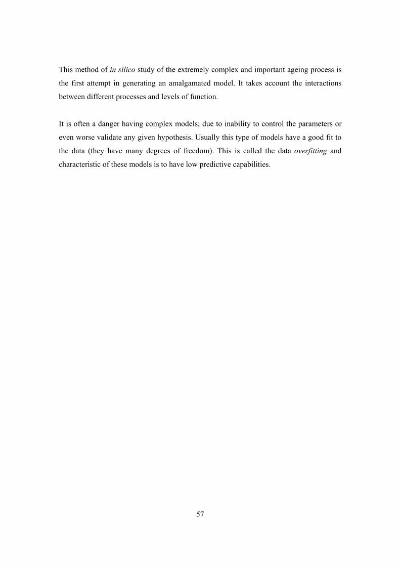
Figure 4.1| Modeling linear and exponential growth of an entity consisting of intact and

damaged proteins .............................................................................................................. 61

Figure 4.2| Symmetrically dividing system ...................................................................... 67

Figure 4.3| Asymmetrically dividing system .................................................................... 67

Figure 4.4| Three level hierarchical model ....................................................................... 72

Figure 4.5| The algorithm.................................................................................................. 74

Figure 4.6| Variation of initial values of Pint and Pdam and their effect on terminal damage

and generation time........................................................................................................... 75

Figure 4.7| Theoretical approach to rejuvenation effect ................................................... 77

Figure 4.8| Symmetrical division ...................................................................................... 79

12

Figure 4.9| Asymmetrical division.................................................................................... 80

Figure 4.10| Damage segregation and size asymmetry causes sibling-specific aging but

increases the robustness of the system.............................................................................. 82

Figure 4.11| Effect of damage segregation on generation time of the mother-cell lineage

in an asymmetrically dividing system............................................................................... 83

Figure 4.12| Effect of damage segregation on size of the mother-cell lineage in an

asymmetrically dividing system ....................................................................................... 84

Figure 4.13| Effect of damage segregation on damage accumulation of the mother-cell

lineage in an asymmetrically dividing system.................................................................. 85

Figure 4.14| Effects of asymmetries on population fitness upon increasing rates of

damage production............................................................................................................ 87

Figure 4.15| S.pombe progression through cell cycle ....................................................... 89

Figure 4.16| Damaged proteins are segregated during binary fission of S. pombe........... 90

Figure 4.17| S. pombe display sibling-lineage specific aging ........................................... 91

Figure 4.18| Extract of typical pedigree tree..................................................................... 92

Figure 4.19| Simplified pedigree tree................................................................................ 93

Figure 4.20| Asymmetrical division without retention ..................................................... 95

Figure 4.21| Asymmetrical division with retention .......................................................... 96

Figure 4.22| Symmetrical division without retention........................................................ 97

List of Tables Table 4.1| Parameters of the single-cell model, their default values and assumptions made................................................................................................................................. 65 Darren Wilkinson

13

14

15

1. Systems Biology The term Systems Biology appeared first time in 1966, when Mihajlo Mesarovic

organized a “Systems Theory and Biology” symposium at Case Institute of Technology

in Cleveland, Ohio. Even though more then 40 years past since that meeting, we consider

that field of Systems Biology is still in its infancy.

The rapid progress in molecular biology of accurate, quantitative experimental

approaches, high-throughput measurements, created a fruitful foundation for a new

discipline. Yet, the identification of all components of the system doesn’t give us an

answer how the system works. Systems biology today combines the knowledge from

various disciplines. Complementing biological reasoning, together with mathematics,

physics, chemistry and computer science we are trying to resolve the complexity of

biological systems.

A cell contains a countless numbers of molecules which interact in a very complex,

sometimes in seemingly random fashion, and yet hold enough information to recreate

another organism. Putting all the pieces together is like solving gigantic puzzle and

represents one of the biggest scientific challenges of this century. It is likely that these

pieces of the puzzle will never be easily understandable without the assistance of

mathematical modeling.

Use of computational modeling has emerged as a powerful descriptive and predictive tool

that allows the study of complex systems to investigate biological phenomena and is one

of the most important techniques used in biology today. The role of mathematical

modeling and simulations is to generate test hypothesis, design experiments and

experimental data.

Hypotheses generated by in silico experiments are then tested by in vivo and in vitro

studies.

16

1.1 Modeling Biological Systems

Biology is one of the most rapidly expanding and diverse areas in sciences. The problems

encountered in biology are frequently complex and often not totally understood.

Mathematical models provide means to better understand the processes and unravel some

of the complexities.

The aim is to construct the model in the simplest possible way, but sill retaining the most

important features of the system. The good model will be able to agree as closely as

possible with the real world observations of the phenomenon we are trying to model and

at the same time be interrogative.

Depending on the process we want to model, the available data and the goal we want to

achieve, biological processes can be modeled using one of the following methods:

Boolean Networks, Stochastic models or Ordinary Differential Equations.

1.1.1 Boolean Networks The first Boolean networks were proposed by Stuart Kauffman in 1969, as random

models of genetic regulatory networks.

The term Boolean networks refer to abstract mathematical models with large number of

coupled variables. They are often use in understanding phenomena like genetic and

metabolic networks, immune systems and neural networks.

In more formal way we can define a Boolean network as a set of nodes G corresponding

to genes V = {x1, . . . , xn} and a list of Boolean functions F = (f1, . . . , fn). The state of a

node (gene) is completely determined by the values of other nodes at time t by means of

the underlying logical Boolean functions. The model is represented in the form of

directed graph. In this approach each variable has two states: ON and OFF, more

specifically, each xi is the expression of a gene, with possible values 1 or 0, which give

17

either expressed or not expressed gene; while F represents the rules of the regulatory

interactions between genes. In this way the system will deterministically go from one

state to another. An advantage of this method is fast computation time, but a draw back

is that variables are discrete and there is no precise notation of time. Since, the Boolean

network reaches a steady state from any initial state; this approach is mainly applicable in

systems where steady state is reached.

1.2.1 Stochastic Modeling

Stochastic Modeling represents a very comprehensive modeling approach in which each

variable represents the number of molecules. A stochastic model is a tool for estimating

probability distributions of the system over time by repeating the simulations many times.

One simulation gives one potential behavior of the studied system. Distributions of

potential outcomes are derived from a large number of simulations (stochastic

projections) which reflect the random variation in the input. If the set of possible states is

continuous then instead of probabilities stochastic process can be described by probability

densities.

One of the most commonly used algorithm for simulating stochastic processes in

continues time and discrete state space is the Gillespie algorithm (Gillespie, 1976). Each

run makes one possible realization; repeating the simulation many times allows us to

estimate the statistical properties of the process (mean behavior, time correlations,

probabilities for certain kinds of behavior).

Stochastic modes describe biological processes more accurately then the Ordinary

Differential Equation approach, but the main drawback is that computation time is very

intensive. Due to this reason they are often replaced by deterministic calculations.

18

1.2 ODE models

Since in building the models for biochemical systems, often for a given input, the output

has to be determine, the equations we use are deterministic (i.e there is a mapping

function f, such that y=f(x), y being the output, and x is the input values).

One of the mostly used model techniques in modeling biological systems is the

Differential Equation approach. If the changes in the system are only time dependent

then we consider the differential equation of type 1 1i

i n ldx

f ( x , ..., x , p , ..., p ,t )dt

= and

refer to it as Ordinary Differential Equation (ODE). The main characteristic of ODEs is

that we can obtain deterministic time series for the variables under investigation. Linear

ODE can be solved analytically, while non-linear ODEs are much harder, and in some

cases it is impossible to find the solution analytically. In this case the approximate

solution is derived using numerical algorithms for solving differential equations. One of

the most elementary methods for solving ODEs numerically is Euler’s forward and

backwards methods (Appendix B.1).

Since in life the most interesting things are quite complicated, and we are trying to model

living systems – most of the biochemical pathways are modeled using non-liner ODEs.

Here, we start by introducing the classical biochemical reaction, well – known Michaelis-

Menten equation, which describes enzyme kinetics.

1 2

1

k kk

E S ES E P−

+ ⎯⎯→ + (1.1)

Where:

1

1

is the enzyme is the substrate, [S] is substrate concentration

is the enzyme-substrate compex is the product is association of substrate and enzyme is dissociation of unaltered substrate fr-

ESESPkk

2

om the enzyme is dissociation of product from the enzymek

19

From the scheme (1.1) we can derive system consisting of 4 ordinary differential

equations:

1 2 1

1 1

1 1 2

2

d [ E ] k [ ES ] k [ ES ] k [ E ][ S ]dt

d [ S ] k [ ES ] k [ E ][ S ]dt

d [ ES ] k [ ES ] k [ ES ] k [ E ][ S ]dt

d [ P ] k [ ES ]dt

−

−

−

= + −

= −

= + −

=

(1.2)

With the following assumptions:

0

[ S ] [ E ][ ES ]

dt=

The rate of production of product P is:

max

m

V [ S ]V

[ S ] K=

+ (1.3)

The equation (1.3) is Michaelis-Menten kintics, where:

2

1 2

1

is maximal velocity of the enzyme and

is Michaelis constant and

max max

m m

V V k ( E ES )k k

K Kk

−

= +

+=

20

Figure 1.1| Michaelis – Menten kinetics

Obtaining the values of Vmax and Km, can be complicated (series of measurements of

initial rates for different initial concentrations), since the rate is non-linear, the non-linear

regression method should be used.

This process can be simplified by transforming Michaelis – Menten equation to obtain a

linear relation between the variables. A commonly used method is Lineweaver-Burk (L-

B) regression method (1.4); where Vmax and Km values can be obtained directly form the

slope of the L-B plot.

1 1 m

max max

Kv V V [ S ]= + (1.4)

A plot, 1v

vs. 1[ S ]

yields a slope m

max

KV

and an intercept 1

maxV.

It is important to note that the L-B method is very sensitive to data error and it strongly

biased towards fitting the data in the low concentration range. Other methods in use are

Eadie-Hofstee, Scatchard (modification of Eadie-Hofstee method) and Hanes-Woolf.

Approximation achieved with ODE models, considering very fast computational time,

makes this approach widely accepted.

21

1.3 Parameter Estimation in ODE models

While building a model, we make many assumptions, since it is often impossible to

acquire real values for all parameters. In some cases, parameters are not measurable

directly, or there is inconsistency between different labs and strains that are used. In those

cases, we have to estimate ‘unknown’ parameters by fitting the model to experimental

data.

While estimating the parameters we are trying to minimize the error function over the

parameters under investigation. Using the goodness of fit measure we are looking at the

discrepancy between the observed values and the expected values in the model.

Most common methods for estimating parameters for the given model are the Least

Square or the Regression Analysis method described by Gauss in the end of 18th century

and the Maximum Likelihood Estimation developed by Fisher in the beginning of 20th

century.

Note that the Least Square Method is the basic method for parameter estimation. There

are a number of other algorithms that can be also used.

1.3.1 Least Square Method

Usually the experimental data we use when creating the model are accompanied by noise.

Even though all control parameters (independent variables) remain constant, the resultant

outcomes (dependent variables) vary. Therefore, a process of quantitatively estimating

the trend of the outcomes, also known as regression or curve fitting, becomes necessary.

The regression process fits equations of approximating curves to the experimental data.

Nevertheless, for a given set of data, the fitting curves of a given type are generally not

unique. Thus, a curve with a minimal deviation from all data points is desired. This best-

fitting curve can be obtained by the method of least squares.

Consider the data set consisting of n pairs (x1,y1), (x2,y2),…, (xn,yn), where xi is

independent and yi is the dependent variable. Let f(x) be the fitting curve and di= yi – f(xi)

the deviation from each data point.

22

Then the curve that would best fit the data would be:

21

1 1

2[ - )] minumumn n

i ii i

d y f ( x= =

= =∑ ∑ (1.5)

Observe that function f(x) can have many different forms:

a) f(x) = ax+b will give The Least Squares Line method with the necessary

condition of having at least 2 data pairs ( n ≥ 2).

b) f(x)=a+bx+cx2 will give The Least Squares Parabola method with the necessary

condition of having at least 3 data pairs ( n ≥ 3).

c) f(x)=a0+a1x+a2x2+….amxm will give The Least Squares mth Degree Polynomial

with the necessary condition of having at least m+1 data pairs ( n ≥ m+1).

If we consider the simplest regression – The Least Square Line method, the best fitting

curve will be:

2 21

1 1[ - ]

n n

i ii i

d y ( a bx )= =

= +∑ ∑ (1.6)

In order to calculate values for a and b, the first derivative of equation (1.6) needs to be equal to zero:

2

1[ - ] 0

'n

i ii

y ( a bx )=

⎛ ⎞⎜ ⎟+ =⎜ ⎟⎝ ⎠∑ (1.7)

23

2

1 1 1 12

2

1 1

1 1 12

2

1 1

Follows:

n n n n

i i i i ii i i i

n n

i ii i

n n n

i i i ii i i

n n

i ii i

y x x y x

a

n x x

n y x x y

b

n x x

= = = =

= =

= = =

= =

⎛ ⎞⎛ ⎞ ⎛ ⎞⎛ ⎞⎜ ⎟⎜ ⎟ ⎜ ⎟⎜ ⎟−⎜ ⎟⎜ ⎟ ⎜ ⎟⎜ ⎟⎝ ⎠⎝ ⎠ ⎝ ⎠⎝ ⎠=

⎛ ⎞ ⎛ ⎞⎜ ⎟ ⎜ ⎟−⎜ ⎟ ⎜ ⎟⎝ ⎠ ⎝ ⎠

⎛ ⎞ ⎛ ⎞ ⎛ ⎞⎜ ⎟ ⎜ ⎟ ⎜ ⎟−⎜ ⎟ ⎜ ⎟ ⎜ ⎟⎝ ⎠ ⎝ ⎠ ⎝ ⎠=

⎛ ⎞ ⎛ ⎞⎜ ⎟ ⎜ ⎟−⎜ ⎟ ⎜ ⎟⎝ ⎠ ⎝ ⎠

∑ ∑ ∑ ∑

∑ ∑

∑ ∑ ∑

∑ ∑

(1.8)

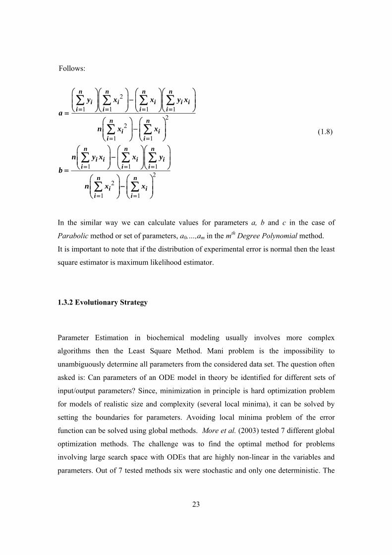
In the similar way we can calculate values for parameters a, b and c in the case of

Parabolic method or set of parameters, a0,…,am in the mth Degree Polynomial method.

It is important to note that if the distribution of experimental error is normal then the least

square estimator is maximum likelihood estimator.

1.3.2 Evolutionary Strategy

Parameter Estimation in biochemical modeling usually involves more complex

algorithms then the Least Square Method. Mani problem is the impossibility to

unambiguously determine all parameters from the considered data set. The question often

asked is: Can parameters of an ODE model in theory be identified for different sets of

input/output parameters? Since, minimization in principle is hard optimization problem

for models of realistic size and complexity (several local minima), it can be solved by

setting the boundaries for parameters. Avoiding local minima problem of the error

function can be solved using global methods. More et al. (2003) tested 7 different global

optimization methods. The challenge was to find the optimal method for problems

involving large search space with ODEs that are highly non-linear in the variables and

parameters. Out of 7 tested methods six were stochastic and only one deterministic. The

24

best result in obtaining the true parameters was accomplished with the SRES method.

One of the best and most widely used is an Evolutionary Strategies based algorithm,

namely Evolutionary Strategy using Stochastic Ranking (SRES, Runnarsson et al. 2000).

Stochastic Ranking is based on a bubble-sort algorithm and is supported by the idea of

dominance. During the evolutionary search the balance between the objective and penalty

function is automatically obtained. Problem with this method that it has a worst-case

complexity O(n2).

25

1.4 Sensitivity Analysis

As shown earlier, designing a mathematical model for biological systems is a circular

process, where the main focus is on the parameters and the variables that are

characterizing the chosen process.

The simplest definition of sensitivity analysis would be that we are observing the effect

on the system after changing the parameters.

Together with parameter estimation, systems analysis is one of the most important and at

the same time the most difficult and laborious steps in modeling procedure.

Performing the sensitivity analysis we can get more information about our model. Some

of the questions usually asked are: which parameters have the highest influence on

system behavior or on the other hand which ones do not have any effect on the system, so

they don't have to be considered further and can be fixed to some arbitrary value.

The main goal of sensitivity analysis is to better understand the dynamic behavior of the

system.

Due to the difficulties in obtaining the quantitative values of certain parameters or if the

modeler is not certain when choosing some parameter values, it is necessary to use

estimates. Sensitivity analysis will ‘show’ the level of accuracy of parameters one should

use to make a model that is useful and valid. Experimenting with a wide range of values

will lead us into behavior of a system in extreme situations. Discovering that the system

behavior greatly changes for a change in a parameter value, we can identify a parameter

whose specific value can significantly influence the behavior mode of the system.

26

As we already noted, sensitivity usually refers to single parameter changes: how does

input signal x change output signal y. This can result in 3 levels of sensitivity:

1. High sensitivity

x has a strong effect on y (usually implies that is hard to estimate values for x)

2. Low sensitivity

x has a no effect on y (usually implies that is easy to estimate values for x)

3. Negative sensitivity

x inhibits y

In the second scenario we generally refer to as a robust system (y is robust against the

changes of x).

In contrast to single parameter change, it is possible to change several parameters at once.

Then we have multiple parameter change and the combined effect can simply be

measured by summing up the single effect. Note that this holds only in case that

parameter changes are sufficiently small.

1.4.1 Robustness vs. Sensitivity

In some case it is expected that the input parameter doesn’t affect the output greatly,

which can confirm the behavior of the system and on other hand the system is expected to

be sensitive to certain parameters. It is wrong to assume that only sensitive parameters are

‘good’ ones and the ones that can give you the most information about the system. In

many cases, as practice has proved, the robustness is also necessary in order to validate

the model.

A large number of sensitivity analysis methodologies are available in the literature. Like

any method in use, different sensitivity analysis methodologies have their advantages and

disadvantages. Choosing the right method for performing a sensitivity analysis

experiment on a model is therefore a very delicate step that depends on a number of

factors: the properties of the model, the number of input factors involved in the analysis,

the computational time needed to evaluate the model or the objective of the analysis.

27

1.4.2 Overview of common sensitivity measures

Consider the mathematical model: 0F(u,k) = , where k is a set of m parameters and u is a

vector of n output values (McRae et al. ,1982).

Then, the following sensitivity measures can be used:

1. Response from arbitrary parameter variation

u u( k k ) u( k )δ= + −

2. Normalized Response

ii

i

uD

u ( k )δ

=

1. Variance

22 2i i i( k ) u ( k ) u ( k )δ = −

2. Extrema

[ ], [ ]i imax u ( k ) max u ( k )

These measures are often use when the model is run for a set of sample points (different

combinations of parameters).

28

1.5 Standardization of biochemical models

The rapid development in the field of systems biology led to enormous expansion of

computational tools that can be used for system analysis. Most of the tools are freely

available for the scientific community and their use will greatly depend on the user’s

preferences and expertise (Klipp et al., 2007).

The vast amount of mathematical models resulted in a need of creating standards for their

systematic organization. One such standard is MIRIAM - Minimum Information

Requested in the Annotation of biochemical Models. It is composed of three parts:

reference correspondence, attribution annotation, and external resource annotation.

Each of these 3 parts deals with specific requirements which a standardized model has to

fulfill. The model has to be encoded in a standardized machine – readable format, where

all the components have to be defined and annotated appropriately using Uniform

Resource Identification (URI).

Standardization of machine-readable format is achieved through Systems Biology

Markup Language (SBML). It is an XML based language and the main purpose is

encoding and exchanging quantitative biochemical models in Systems Biology. The

original specification (Level 1) aimed mainly at continuous deterministic models.

Whereas, the current specification (Level 2) is perfectly capable of encoding discrete

stochastic models in an unambiguous way.

Models of arbitrary complexity can be represented and each type of components is

described using specific data types. More information regarding structure, development

and additional tools is available on the developer’s web site www.sbml.org.

29

Age is an issue of mind over matter. If you don't mind, it doesn't matter.

Mark Twain

2. Biology behind equations

2.1 Ageing: definitions and history

Aging is the process, which intrigues people since the ancient time. Finding the aging

formula and a possibility of controlling it represents the incredible challenge and

motivation. One of the first fictions written - Epic of Gilgamesh - has a main focus on

immortality. History is full of individuals whose life was driven by the force of finding

the fountain of youth – a legendary spring that restores the youth. And where we are

today? Are we just modern Gilgamesh, with improved tools, techniques and hopefully

more knowledge, but with the same goal? Is it true that we want to live indefinitely?

Laws of physics are pretty simple and sometimes harsh: “over time differences in

temperature, pressure, and density tend to even out in a physical system that is isolated

from the outside world”. This is the Second Law of Thermodynamics and in principal

explains irreversibility in nature. So, immortality, defined as ‘possibility of repair and

incapability of dying’ is not possible. The other term in use, indefinite lifespan, might be

more appropriate, since it implies freedom from death by age.

What is then our goal? To make old people healthier. As simple as that. To have a

generation that will enjoy in their elderly life, without being burden for society. Already

today, there is evidence to suggest that not only are we living longer, we are staying

healthier until an older age - something health experts refer to as 'compression of

morbidity', meaning that most of us will only suffer severe age-related illnesses in the last

years of life.

30

Defining ageing is complicated as the ageing process itself is. There is no the definition,

but rather a series of descriptive observations which together can give us some glimpse

how we see the ageing phenomena. One of the descriptions commonly used is that

‘ageing is simply the age or time dependent changes that occur to biological entities’

(Medawar, 1952). But, this doesn’t give us an answer how and why changes arise.

2.2 Yeast as a model organism

To come closer of solving the mystery of human ageing, we have to start from simpler

organisms. Yeast in general has been accepted as very powerful model to study various

biological processes. Advantages are numerous: it is relatively easy to culture them, do

genetic manipulations, experimental tools to analyze their biochemical and physiological

functions are established. Of the great importance is the fact that it has its full genome

annotated, that generation time is fast, and also very important aspect that is relatively

cheap to use.

In the course of this work, two yeast species were studied Saccharomyces cerevisiae and

Schizosaccharomyces pombe.

2.3 Cell division

2.3.1 Asymmetricaly dividng systems - Saccharomyces cerevisie

Saccharomyces cerevisie (baker’s yeast or budding yeast) is one of the simplest

eukaryotic organisms. In the spring of 1996, the complete genome sequence of the S.

cerevisiae was obtained, making yeast the first eukaryotic organism to be completely

sequenced.

It is a small, single-cell fungus. Like other fungi, it has rigid cell wall and mitochondria

but not chloroplast. It reproduces almost as fast as bacteria. Most fundamental cellular

processes are conserved from S. cerevisiae to humans and have first been discovered in

yeast. There are many basic biological properties that are shared. About 20 percent of

human disease genes have counterparts in yeast. This suggests that such diseases result

from the disruption of very basic cellular processes, such as DNA repair, cell division or

31

the control of gene expression. It also means that we can use yeast to look at functional

relationships involving these genes, and to test new drugs.

S.cerevisiae divides in a way that is not very common in nature. Buds (future ‘daughter’

cell) may arise at any point on the existing cell surface (referred to as ‘mother). Buds are

formed when the mother cell has attained a critical size. After cell division a

characteristic bud scar is left on the surface of the mother cell (Figure2.1).

Figure 2.1| Accumulation of bud scars. Upper panel is schematic representation of bud

scars appearance on mother’s cell surface during successive division. Lower panel is

calcoflour staining of bud scars (graphical representation courtesy of Nika Erjavec).

Since the new born daughter has a smaller size then its mother, it will require longer

generation time to attain a critical size before it in turn becomes mother itself (Figure2.2).

However, this unconventional way of division and clear asymmetry between mothers and

daughters, makes it an excellent model for studying ageing. But this is not the only

prerequisite for studying ageing. Bakers yeast has been established as model for cellular

ageing in 1959 when Mortimer and Johnston discovered that individual yeast cells are

mortal.

32

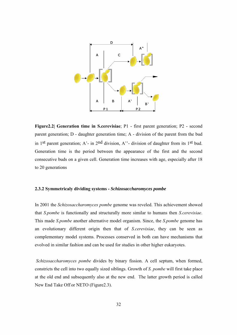
Figure2.2| Generation time in S.cerevisiae; P1 - first parent generation; P2 - second

parent generation; D - daughter generation time; A - division of the parent from the bud

in 1st parent generation; A’- in 2nd division, A’’- division of daughter from its 1st bud.

Generation time is the period between the appearance of the first and the second

consecutive buds on a given cell. Generation time increases with age, especially after 18

to 20 generations

2.3.2 Symmetricaly dividing systems - Schizosaccharomyces pombe In 2001 the Schizosaccharomyces pombe genome was reveled. This achievement showed

that S.pombe is functionally and structurally more similar to humans then S.cerevisiae.

This made S.pombe another alternative model organism. Since, the S.pombe genome has

an evolutionary different origin then that of S.cerevisiae, they can be seen as

complementary model systems. Processes conserved in both can have mechanisms that

evolved in similar fashion and can be used for studies in other higher eukaryotes.

Schizosaccharomyces pombe divides by binary fission. A cell septum, when formed,

constricts the cell into two equally sized siblings. Growth of S. pombe will first take place

at the old end and subsequently also at the new end. The latter growth period is called

New End Take Off or NETO (Figure2.3).

33

NETO

NO

Figure2.3| Growth of Schizosaccharomyces pombe. Schematic representation of

S.pombe progression through cell cycle. In blue accumulation of bud necks is presented.

(graphical representation courtesy of Nika Erjavec).

34

2.4 Ageing in Yeast

As previously noted, ageing in S.cerevisiae has been reported 50 years ago. Yeast shows

the same exponential decline in fitness and fecundity over time, as many other higher

eukaryotes. The mortality curves follow the Gompertz-Makeham law (see Chapter 3 for

more details) (Figure2.4).

Figure2.4| Mortality curves. Survival by age, know as mortality curve, for humans and

yeast.

Yeast lifespan can be measured in two ways:

Replicative lifespan is defined as the number of divisions an individual yeast cell

undergoes before dying. It is expressed in generations (it is limited) and it is measured by

growth on agar plates and micromanipulation. (Figure 2.5A)

Chronological lifespan (survival in stationary phase), is the time a population of yeast

cells remains viable in a non-dividing state following nutrient deprivation. It is expressed

as time and measured by growth in liquid. (Figure 2.5B)

35

generations

% s

urvi

val

time

% s

urvi

val

A B

Figure2.5| Replicative and chronological life span in yeast.

There is no strong correlation between chronological and replicative lifespan. It has been

shown that the chronological lifespan can be noticeably extended without altering the

replicative lifespan.

When studying yeast ageing we are mainly focused on replicative lifespan.

Figure 2.6| The spiral model of yeast ageing (Adapted from Jazwinski, et al Exp Geront 24:423-48 (1989))

“virgin” cell

daughter1

1st

Generation (cell cycle)

dead cell(lysis)

nth

daughtern

AGING

Lifespan = n (20-40)

36

From the mortality curves we can define mean and maximum lifespan:

Mean lifespan (average lifespan) corresponds to the age at which the horizontal line for

50% survival intersects the survival curve.

Maximum lifespan corresponds to the age at which the survival curves touch the age-

axis (0% survival) - and this represents the age at which the oldest known member of the

species has died.

For wild-type (wt) laboratory yeast strain, the mean lifespan is approximately 25

divisions, while the maximal is around 40 (Figure2.6). Those numbers should not be

taken too exact, since lifespan can vary due to the numerous reasons: different labs,

different strains.

A mother cell undergoes many typical changes during her life time, such as: sterility,

slowing of the cell cycle, appearance of surface wrinkles, blebs and bud scars, dramatic

increase in cell size, loss of asymmetry, fragmentation of nucleus.

It has been believed that the accumulation of bud scars can limit the replicative potential

in yeast. However, buds occupy only 1% of the mother’s surface, and even expanding the

available surface would not lead to an increased lifespan. Also, there are reports that new

buds can grow from existing scars.

One of the most obvious signs of an old yeast cell is the increase in size. Several studies

showed that the volume of a mother cell increases linear with age. Along with size, cell

cycle increases exponentially with generation time, as well.

Due to the clear size-symmetry, S.pombe, was not considered as ageing model until 1999

when it was reported that fission yeast has a finite lifespan.

It was believed that this organism doesn’t age, since the division is symmetrical, and the

two produced siblings will be completely identical. The similar arguments were applied

for bacterium Escherichia coli. Recent work by M. Ackermann (2003) and E. Stewart

(2005) purposed that Caulobacter crescentus and E.coli display replicative senescence

e.g. one sibling stops dividing after accomplishing certain number of division, while the

other continuers to divide normally.

37

“Tomorrow you may be younger.”

2.5 Ageing theories

Since the beginning of ageing research more then 300 theories have been postulated. The

key requirement for a good ageing theory would be the necessity of having high

predictive and explanatory power. At the beginning of ageing research scientist were

looking for the one and only theory – the theory – the one that would give complete

understanding of the highly complex ageing process. Even there have been discussion

could we called it ageing process? Is it a process? By general definition process is “a

series of actions, changes, or functions bringing about a result” it can also be “a natural

phenomenon marked by gradual changes that lead toward a particular result”. The

common thing for all those definitions is that it is something that has a beginning and an

end. And ageing indeed has a starting point – new cells are created over and over again,

and an end point is the death of the cell itself. Death as a final result of series of changes

that cell goes through.

In general, ageing theories can be summarized in two groups:

1. Programmed Theories

2. Error Theories

The main idea behind Programmed Theories is that cells are designed to age. Ageing is

due to something inside an organism's control mechanisms that forces elderliness and

decline.

The other, more accepted – Error Theory postulates that ageing is caused by

environmental damage to the cells, which accumulates over time. It can be damage due to

radiation, chemical toxins, metal ions, free-radicals, hydrolysis, disulfide-bond cross-

linking, etc. Such damage can affect genes, proteins, cell membranes, enzyme function

and blood vessels.

38

One of the first Error Theories was Orgel’s Error Catastrophe (1963). The theory

suggests that copying errors in DNA and the incorrect placement of amino acids in

protein synthesis could aggregate over the lifetime of an organism and eventually cause a

catastrophic breakdown in the form of obvious aging. This theory has been dismissed

since the experimental verification always gave negative results.

Other error theories include wear and tear theory – cells and tissues simply wear out over

time, rates of living – the oxygen usage is faster in some organisms, therefore they live

shorter.

In this chapter will give brief overview of some of the most studied and further developed

theories.

2.5.1 Free Radical theory

Following the idea of R. Gerschman that free radicals are toxic agents, D. Harman

purposed in 1954 the Free Radical Theory of Ageing. In general, this theory presumes

that there is an accumulation of free radicals over time. Under the name free radicals we

often assume reactive oxygen species (ROS). ROS molecules are highly reactive and as

such can damage all sorts of cellular components. The ability to cope with ROS decreases

with age. One form of this theory – accumulation of damaged proteins is discussed in

section 2.6.

2.5.2 Disposable soma theory

Based on the fact that both somatic maintenance and reproduction require energy, the

disposable soma theory postulates that there is a negative correlation between

reproduction and repair. This theory predicts that aging is due to the accumulation of un-

repaired somatic defects and the primary genetic control of longevity operates through

selection to increase or decrease the investment in the basic cellular maintenance systems

in relation to the level of environment hazard. Also, a high level of accuracy is

39

maintained in immortal germ line cells, or alternatively, any defective germ cells are

eliminated.

2.5.3 ERCs

In 1997, Sinclair and Guarente proposed that yeast ages due to gradual accumulation of

extrachromosomal ribosomal DNA circles (ERCs). In S.cerevisiae ERCs are located on

the XII chromosome. Unsilenced rDNA have an increased frequency of recombination

events and homologous recombination in this region can lead to the formation of

extrachromosomal rDNA circles (ERCs). Since ERCs contain an origin of replication,

they can self-replicate (Figure 2.7). Interestingly, ERCs are asymmetrically inherited by

the mother cell at the time of cytokinesis. Furthermore, overexpression of ERCs shortens

lifespan (Sinclair and Guarente, 1997). Therefore, ERCs have been proposed to be a

senescence factor.

Deletion of ribosomal DNA (rDNA) repeats results in the formation of ERCs. Since

ERCs are able to replicate independently during S-phase, they can accumulate much

faster then chromosomal DNA. During the budding process ERCs are retained in the

mother cell, leaving the daughters ERC-free, which in turn give an immortal yeast

population. When a mother cell gets close to its replicative life, the mechanism for ERC

segregation starts malfunctioning which results in daughters that inherit small amounts of

ERCs. Because, the level of ERCs is still too low, this prematurely old daughters are

capable of producing healthy daughters.

40

Figure2.7| Formation of extrachromosomal ribosomal DNA circles (ERCs). In

budding yeast ERCs are accumulated over mother cell life span and are segregated

asymmetrically between progeny and progenitor.

The reason why this theory is not widely accepted is the fact that ERCs accumulation is

only observed in S.cerevisiae and it is believed that it can not explain ageing in higher

eukaryotes.

2.6 Accumulation of damaged proteins

The Free Radical Theory indicates the key role of ROS in the ageing process. ROS

damages cellular components and can cause oxidative damage to cellular

macromolecules (proteins, carbohydrates, lipids and nucleic acids) which in turn become

cytotoxic. According to Free Radical Theory, ageing is caused by the gradual

accumulation of un-repaired molecular damage, leading to an increasing fraction of

damaged cells and, eventually, to functional impairment of tissues and organs.

41

Native proteins can become reversibly and/or irreversible oxidatively damaged. The

reversible ones are repaired by specific enzymes. The repair mechanism is present in

cytosolic and mitochondrial compartments. The rest of the proteins are irreversibly

damaged and there is no evidence of their repair mechanism. They are eliminated either

via degradation pathways or become aggregates. The degradation pathways are part of

the cytosol and mitochondria and are regulated by 20S proteasome, lysosome and Lon

protease respectively (Figure2.8).

Figure2.8| Different modes of protein degradation.

An age - related increase in the level of oxidatively modified proteins disrupts the balance

between the rate of protein oxidation and the rate of elimination of oxidized proteins. As

long as the balance is kept the cell is viable.

Protein carbonylation negatively affects cellular performance in two ways; (i) the

modification causes structural aberrancies and abrogates the targeted proteins’ catalytic

42

functions and (ii) triggers formation of high molecular, potentially cytotoxic, aggregates

that, among other things, may impede protease activity.

Inability of the cell to eliminate oxidatively damaged proteins causes the buildup of

damaged proteins, which becomes a burden for the cells and lead to cell death.

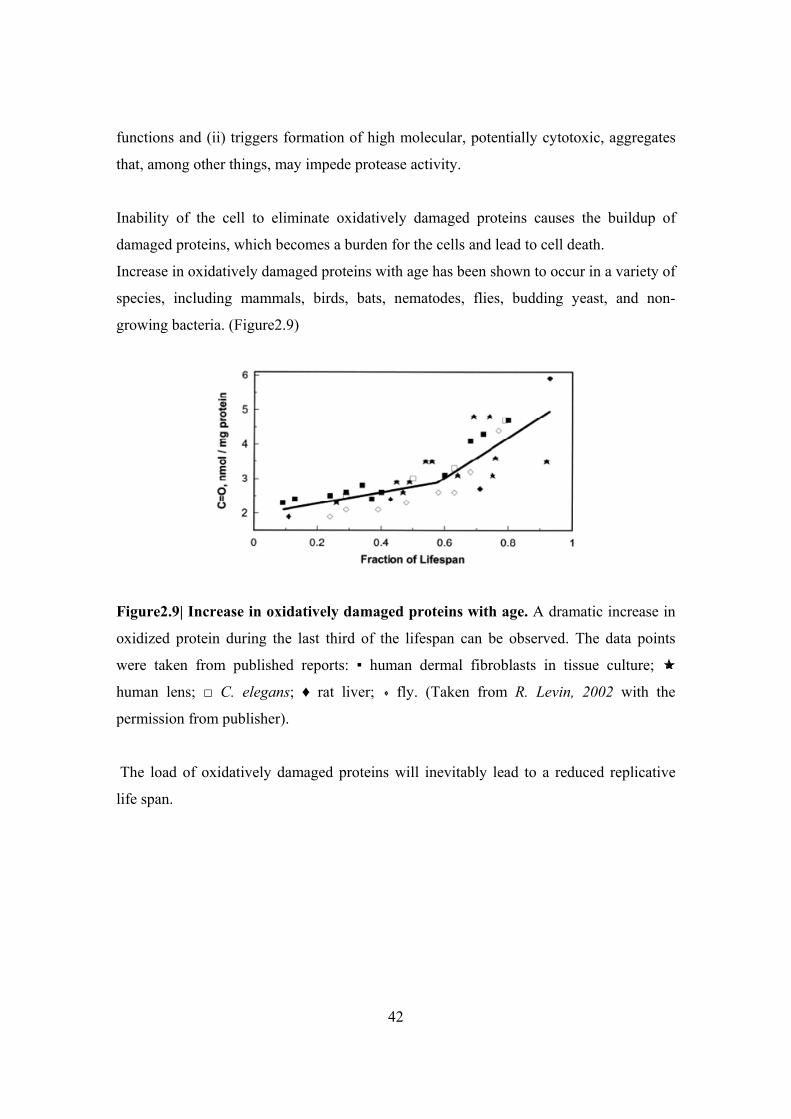
Increase in oxidatively damaged proteins with age has been shown to occur in a variety of

species, including mammals, birds, bats, nematodes, flies, budding yeast, and non-

growing bacteria. (Figure2.9)

Figure2.9| Increase in oxidatively damaged proteins with age. A dramatic increase in

oxidized protein during the last third of the lifespan can be observed. The data points

were taken from published reports: ▪ human dermal fibroblasts in tissue culture;

human lens; □ C. elegans; ♦ rat liver; fly. (Taken from R. Levin, 2002 with the

permission from publisher).

The load of oxidatively damaged proteins will inevitably lead to a reduced replicative

life span.

43

2.7 Damage retention Accumulation of oxidized proteins has been shown to occur during mother cell-specific

ageing, starting during the first G1 phase of newborn cells.

It has been shown that oxidatively damaged proteins are inherited asymmetrically during

yeast cytokinesis such that most damage is retained in the mother cell (H. Aguilaniu,

2003) (Figure2.10). In other words, proteins that are oxidatively damaged are retained

within the mother cell, leaving its daughter virtually damage free. The process was shown

to be dependent on the age determinator SIR2 and on actin polymerization. Deletion of

SIR2 shortens the replicative lifespan while its overexpression prolongs lifespan.

Oxidatively damaged proteins

Young

Oxidatively damaged proteins

Young

Figure2.10| Schematic representation of asymmetrical accumulation of damage

proteins during replicative age in S.cerevisiae. Light pink dots represent low level of

damage, while darker dots show high level of damaged proteins. (graphical representation

courtesy of Nika Erjavec)

The fact that yeast has a limited replicative lifespan implies that each daughter cell

produced must have a full replicative potential. Thus, there is a critical asymmetry at the

time of cell division that ensures the proper segregation of a “senescence factor” (Egilmez

et al., 1990). The nature of this factor is still under intense scientific scrutiny.

44

Figure2.11| Asymmetric distribution of oxidized proteins during cytokinesis in

S.cerevisiae. Representative young, 4-5 and 10.12 generations old dividing mother cell.

Oxidized proteins are detected in situ and here are increasing from red to blue.

In S.cerevisiae age-dependent oxidation targets most proteins and most oxidized proteins

are accumulated to the same extent in the mother cell. Segregation of oxidized proteins is

a result of active retention in the mother cell.

Overall double increase in carbonylation in old mothers and in the daughters of old

mothers, compared with unsorted culture, implies that asymmetric distribution of

oxidatively damaged proteins take place between mother and bud in aging yeast cells.

(Figure 2.11 and Figure 2.12).

Figure2.12| Levels of oxidative protein damage as a function of replicative age.

Average number of birth/bud scars (open bars); Protein carbonyl levels (filled bars).

Taken from H. Aguilaniu (2003) with the permission from publisher.

45

2.8 Rejuvenation

The verb rejuvenation (re + Latin juvenis – young) means to become/make young or

youthful again. Rejuvenation, even though opposite from ageing, complements the ageing

process and is an inevitable aspect of aspiration to have an immortal population.

The altruistic concept of having a system that will for the benefit of the population entrust

the off-spring that is intact of any sort of damage is one of the most striking biological

phenomena.

The whole concept of ageing research can then be formulized in one yet obvious, but

very complex question: “How something old can generate something young?”(Thomas

Nyström)

In S.cerevisiae, as previously stated, a mother cell produces an off-spring that is born

damage-free with full replicative potential.

Figure2.13| Rejuvenation. The old mother cell produces a prematurely old daughter,

whose replicative potential is equal to the remaining mother’s life span. Remarkably,

daughters born from these old daughters, display normal replicative life span.

46

As a mother cell becomes older, the newly produced daughters are born prematurely old

– indicating that asymmetry in protein damage, together with loss of size asymmetry has

broke down. This suggests that daughters of old mothers have inherited a senescence

factor. However, the striking thing is that the daughter of prematurely old daughters will

have full replicative potential and no damaged proteins (Figure2.13)

47

3. Modeling Ageing in Yeast 3.1 ERC model A mathematical model of Extrachromosomal Ribosomal DNA Circles (ERCs)

accumulation in yeast developed by Colin Gillespie, relays on observations from D.

Sinclair and L. Guarente that the number of ERCs is unevenly distributed between

mother and daughter cell during replicative age.

The biological description of this process is given in Chapter 2.

Here we give mathematical interpretation based on the Gillespie model. The ERC model

is stochastic model composed of 3 main parts.

1. ERC generation:

The cell can acquire the ERC in 2 different ways:

a) through excision from the chromosome

b) through inheritance from its mother

The first step is known to appear randomly with low frequency. It holds that

Pfor = min( αi xi, 1), for i = 0, 1, 2 (3.1)

Pfor is the probability of generating new ERC in a ERC-free mother cell

x is the number of completed generations

αi is a constant

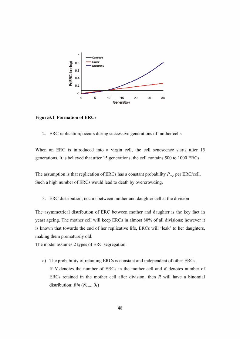
Introducing generation constrains, we can obtain 3 possible cases (Figure3.1):

i = 0 → means that the probability of generating ERCs is age-independent.

i = 1 → means that the probability of generating ERCs has a linear increase with age

i = 2 → means that the probability of generating ERCs has a quadratic increase with

age

48

Figure3.1| Formation of ERCs

2. ERC replication; occurs during successive generations of mother cells

When an ERC is introduced into a virgin cell, the cell senescence starts after 15

generations. It is believed that after 15 generations, the cell contains 500 to 1000 ERCs.

The assumption is that replication of ERCs has a constant probability Prep per ERC/cell.

Such a high number of ERCs would lead to death by overcrowding.

3. ERC distribution; occurs between mother and daughter cell at the division

The asymmetrical distribution of ERC between mother and daughter is the key fact in

yeast ageing. The mother cell will keep ERCs in almost 80% of all divisions; however it

is known that towards the end of her replicative life, ERCs will ‘leak’ to her daughters,

making them prematurely old.

The model assumes 2 types of ERC segregation:

a) The probability of retaining ERCs is constant and independent of other ERCs.

If N denotes the number of ERCs in the mother cell and R denotes number of

ERCs retained in the mother cell after division, then R will have a binomial

distribution: Bin (Nmax, θ1)

49

b) The number of ERCs can be retained with 2 different probabilities.

The first Nmax ERCs are retained with probability θ2, and above Nmax with

probability 0.5 (equal distribution of ERCs between mother and daughter), then

1

1 2

maxR N NR

R R≤⎧

= ⎨ +⎩

,

if otherwise,

(3.2)

And, R1 and R2 have two independent binomial distributions:

Bin(Nmax, θ2), Bin(N - Nmax, 0.5), respectivly.

The results suggest that having a quadratic increase in probability would fit the best to

experimental studies. (Figure 3.2)

Figure 3.2| Agreement with experimental data.

Also, the segregation of ERCs breaks down in older mother cells and the formation of

ERCs cannot be constant (red curve; gives long lived cells (~120 generations), but rather

depends on the age of the yeast cell. This suggests that there must be another

mechanism(s), in addition to ERC accumulation which underlies yeast ageing.

50

This theory can explain the fact that an old mother will give rise to old daughters, and

that a daughter of an old daughter will have full replicative potential (e.g. born ERC-

free).

51

3.2 Disposable Soma model for Ageing The main aspect of the Disposable Soma theory is that there is a balance between somatic

maintenance, reproduction and growth (Kirkwood, 1977). In Chapter 2 there is a insight

to the biological background of the mathematical model developed by Kirkwood and

Drenos (2004).

The Disposable Soma model is based on Euler- Lotka (1) and Gompertz-Makeham (3)

equations.

3.2.1 Euler – Lotka equation

Linking the proportional growth rate of a population to the characteristic functions that

define life history is an old problem, originally solved by Euler (1760), rediscovered in

the context of modern population genetics by Lotka (1907), and first applied by Fisher

(1930). Surprisingly, the problem has no algebraic solution, and r must be defined

implicitly by an integral equation. The parameter r was dubbed by Fisher the Malthusian

parameter, and the equation from which it is computed is referred to as the Euler-Lotka

equation:

1rxe l( x ,s )m( x,s )dx−=∫ (3.3)

Where:

is intrinsic rate of natural selection is survivorship function (a proportion of population remaining alive at age ),

depends on maintenance is fertility function (the mea

rl( x , s ) x

sm( x,s ) n number of offsprings produced per time unit time at age ), depends on maintenance x s

If we assume that r is known, then we can compare the relative contributions to growth of

offspring produced at different times: their value declines exponentially with time at the

prescribed rate r. The r is then, the rate which reduces the total reproductive value of all

offspring to unity.

52

With computational techniques that have become commonplace, the numerical

determination of r is fast and straightforward. The algorithm is seeded with a first guess

for r, which is used to evaluate the integral numerically. The difference between the

computed result and unity is fed into a Newton-Raphson or equivalent algorithm for

generating a next-closer value of r, and the procedure is iterated until the desired

accuracy attains.

Hamilton (1966) showed that the selection pressures acting on life history are best

measured by the sensitivity of r to changes in fecundity or instant survival rate.

Alleles that influence life history such that r is increased spread at a faster rate than other

alleles and invade the population. Alleles acting late in life experience affect r less

strongly and thus experience a weaker selective pressure than alleles acting early in life.

This has three evolutionary consequences:

(1) Alleles that increase early survival or fertility at the cost of late survival or fertility

tend to be favored.

(2) Deleterious alleles that decrease early survival or fertility will be more strongly

selected against than alleles that decrease late survival or fertility.

(3) Beneficial alleles that increase early survival or fertility will be more strongly favored

than alleles that increase late survival or fertility.

Consequently, it is expected that the survival or fertility rate will decrease with age (at

least once sexual maturity is reached).

53

3.2.2 Gompertz – Makeham law of mortality In 1825 Benjamin Gompertz proposed that death rate exponentially increases with age:

0Gxm( x ) A e= (3.4)

Where:

is mortality rate as a function of time or age is extrapolated constant to birth or maturity (basal vulnerability)

is exponential Gompertz mortality rate coefficient (acturial ageing rate)o

m( x )AG

Often, A0 is replaced with A – the initial mortality rate (IMR), and G with the mortality

rate doubling time (MRDT), equal to ln2/G. In humans MRDT is 8 years, meaning that

after our sexual peak, chances of dying double every 8 years.

This version of Gompertz law is used in protected environments, such as laboratory

conditions, where the probability of external causes of death is low. If, we are looking for

the mortality rate in natural environment then, a new parameter need to be included in the

equation – the Makeham parameter M0, which then represents, the age – independent

component of the Gompertz – Makeham equation (3), in the contrast to the Gompertz

function which is an age-depended component.

0 0Gxm( x ) A e M= + (3.5)

3.2.3 The disposable soma model

Using above mentioned equations, the mathematical model incorporates the main ideas of

disposable soma theory, such as maintenance, fertility and fitness.

In general, the model confirms the principles of disposable soma theory, which states that

‘the organism should not waste resources by extending life span potential beyond what is

likely to be seen in wild populations subject to external mortality’. Kirkwood and Drenos

suggest that modeling disposable soma theory, survivorship l(x) can simply be increased

by increasing investment in maintenance s. While the increase in fecundity m(x), cannot

54

simply be achieved with increase in s and will lead to postponed maturity, diminishment

of the peak reproductive rate and slowing of the age-related decline.

The model also predicts that there is a balance between growth and reproduction in one

hand and maintenance on the other, and that increase in maintenance will lead to decrease

in growth and reproduction.

55

3.3 Network theory of ageing Another model purposed by Kirkwood and Kowald in 1995 integrates the contribution of

defective mitochondria, aberrant proteins and free radicals as major players in the ageing

process. Suggestions that ageing is result of multiple factors that work together formed

the network theory of ageing. This fact would lead to greater predictive and explanatory

capabilities then observations derived from a set of individual models. However, this

approach makes many assumptions and simplifies some of the process in order to

reconcile mathematical and biological complexity.

The model is also known as MARS model, which stands for mitochondria, aberrant

proteins, radicals, scavengers (Figure3.3)

Figure3.3| Schematic representation of components of the MARS model. (adapted from Kowald A, Kirkwood TBL (1993))

56

The role of mitochondria is a central part of the model. Some of the functions modeled

are mitochondria as ATP source, production of free radicals, mitochondrial replication

and turnover. The fact that more radicals and less ATP are produced by damaged

mitochondria is modeled trough different damaged classes. Various parameters describe

different rates of mitochondrial replication, depending whether it is intact or damaged.

The second component of the MARS models is integrated in one and comprises of free

radicals, aberrant proteins and antioxidants. A feedback loop controls the rate of synthesis

of proteins and the assumption is that synthesis is regulated by product inhibition. Also,

during protein synthesis, proteins can be damaged or their activity or specificity can be

affected. Scavengers and antioxidants are regulated by substrate activation and the

ribosomes by autoinhibition.

The full model consists of 35 differential equations and number of parameters. Such a

large model generates a huge number of parameter combinations and simulations.

The MARS model explains the following observations and experimental findings:

1. the loss of specific enzyme activity; demonstrated by sharp increase of inactive

proteins with age.

2. a decline in enzyme specificity

3. the significant increase in protein half-life with age

4. a decrease in mitochondria population with age

5. an increase of the fraction of mitochondria with age

6. an increase in the average rate of free radical production per mitochondria with

age

7. a decrease in the average level of ATP generation per mitochondria with age

57

This method of in silico study of the extremely complex and important ageing process is

the first attempt in generating an amalgamated model. It takes account the interactions

between different processes and levels of function.

It is often a danger having complex models; due to inability to control the parameters or

even worse validate any given hypothesis. Usually this type of models have a good fit to

the data (they have many degrees of freedom). This is called the data overfitting and

characteristic of these models is to have low predictive capabilities.

58

59

4. Mathematical Model of Accumulations of Damaged Proteins

To approach the questions, if there is an advantage of asymmetrical cell division – i.e.

production of cells of different size, different levels of damage, and unequal reproductive

potential, we developed a mathematical model aimed at elucidating effects of cellular

asymmetries on fitness, proliferating capacity, and aging.

The mathematical model consists of a system of ordinary differential equations and a set

of algebraic equations to describe how the accumulation of damaged proteins influences

ageing in yeast. The model we propose has two main features. First, the set of ODEs

describes the behavior of intact and damaged proteins through successive cell

generations. Secondly, we define a set of rules for the distribution of proteins based on

different modes of division and we introduce a retention coefficient that affects the

distribution of proteins between progenitor and progeny.

4.1 Description of system dynamics in between two cell divisions To simulate the proliferation of a simple entity consisting of two types of molecules (e.g.

diffusible proteins), intact and damaged ones, we constructed a mathematical model

based on ordinary differential equations (1). The ODEs describe the accumulation of the

intact (Pint) and damaged (Pdam) proteins, such as oxidatively carbonylated proteins,

during the cell cycle and successive cell generations. The sum (P) of intact (Pint) and

damaged (Pdam) proteins determines the total size of the entity.

60

12 3

3 4

12 4

intint int

s int dam

damint dam

int dams int dam

dP k k P k Pdt k P P

dP k P k Pdt

dP k k P k Pdt k P P

= − −+ +

= −

= − −+ +

(4.1)

The temporal dynamics of intact proteins, Pint is given by a production term (maximal

rate k1) dependent on the current amount of total protein in the cell, the half-saturation

term (rate constant ks), a degradation term (rate constant k2), and a term for the

conversion of intact proteins into irreversibly damaged ones (rate constant k3). The

dynamics of damaged proteins Pdam is ruled by the conversion of intact proteins to

damaged ones (k3) and the degradation of damaged proteins (rate constant k4).

Initially, the numbers of intact and damaged molecules increase until production and

degradation is balanced, such that a steady state is approached (Figure 1A and B). Since

protein and RNA synthesis in unicellular systems has been shown to increase either

exponentially or pseudo-linearly during the cell cycle, we tested both types (linear and

exponential) of cellular growth (Figure 4.1A and B), yielding comparable results when

fitness, aging, and robustness were determined. Note that in the case of modelling

exponential growth of the cell we multiplied the extra term Pint to the growth rate of

intact proteins:

12 3

int intint int

s int dam

dP k P k P k Pdt k P P

= − −+ +

(4.2)

The protein production rate, k1, has been adjusted by hand allowing for a steady state to

be reached and has been assigned a final value of 107. We choose values of k2 and k4, the

degradation rates of Pint and Pdam, respectively, so that k2 < k4. Degradation rates are

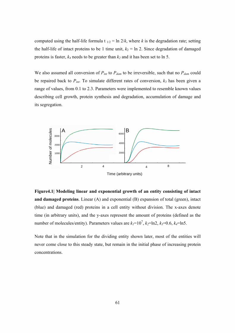
61

computed using the half-life formula t 1/2 = ln 2/k, where k is the degradation rate; setting

the half-life of intact proteins to be 1 time unit, k2 = ln 2. Since degradation of damaged

proteins is faster, k4 needs to be greater than k2 and it has been set to ln 5.

We also assumed all conversion of Pint to Pdam to be irreversible, such that no Pdam could

be repaired back to Pint. To simulate different rates of conversion, k3 has been given a

range of values, from 0.1 to 2.3. Parameters were implemented to resemble known values

describing cell growth, protein synthesis and degradation, accumulation of damage and

its segregation.

3000

2000

1000

6000

4000

2000

Time (arbitrary units)

A B

Num

ber o

f mol

ecul

es

2 4 4 8

Figure4.1| Modeling linear and exponential growth of an entity consisting of intact

and damaged proteins. Linear (A) and exponential (B) expansion of total (green), intact

(blue) and damaged (red) proteins in a cell entity without division. The x-axes denote

time (in arbitrary units), and the y-axes represent the amount of proteins (defined as the

number of molecules/entity). Parameters values are k1=107, k2=ln2, k3=0.6, k4=ln5.

Note that in the simulation for the dividing entity shown later, most of the entities will

never come close to this steady state, but remain in the initial phase of increasing protein

concentrations.

62

4.2 Description of cell division In the present model, cells initiate division once they have attained a critical cell size,

defined by Pint reaching a value called Pdiv, arbitrarily assigned to 1500 molecules/cell in

the present work. The following set of transition equations describes how the proteins are

distributed between progenitor and progeny when the cells divide, i.e. when Pdiv is

reached.

The subsequent equations are derived with following assumptions:

1. Total amount of proteins (P) in the cell would be sum of Pint and Pdam.

2. Sum of, the amounts of intact proteins in the progenitor and the amounts of intact

proteins in progenies are constant before and after division. Similarly for damaged

proteins.

3. Sum of the amounts of intact and the damaged proteins in the progenitor is constant.

Similarly for progenies.

4.2.1 Without damage segregation In the case of a protein distribution that is only dependent on size of the newly generated

cells, the different cell types obtain the following amounts of proteins:

For progenitors:

( ) ( )( ) ( )

( ) ( ) ( )

1

1

1

int int mother

dam dam mother

int mother dam mother

P g P g s

P g P g s

P g P g s P g s

+ = ⋅

+ = ⋅

+ = ⋅ + ⋅

(4.3)

63

For progenies:

( ) ( )( ) ( )

( ) ( ) ( )

1

1

1

int int daughter

dam dam daughter

int daughter dam daughter

P g P g s

P g P g s

P g P g s P g s

+ = ⋅

+ = ⋅

+ = ⋅ + ⋅

(4.4)

The size of the progenitor, smother, denotes the percentage of protein from the previous

generation that is kept in that cell, while the size of the progeny, sdaughter, expresses the

percentage of protein assigned to the new-born cell. P(g+1) denotes the initial amount of

total protein for the new generation (g+1), while P(g) corresponds to the final protein

amount before division of the previous generation g (similarly for damint P,P ).

4.2.2 With damage segregation We next introduce a retention coefficient (re), describing the amount of Pdam being

retained by the progenitor. In this case, segregation of Pdam, and consequently Pint, is

affected by both size and retention, according to the following set of transition equations:

For progenitors:

( ) ( ) ( ) ( )( ) ( ) ( )( )

( ) ( ) ( )

1 1

1 1

1

int int mother dam mother

dam dam mother mother

int mother dam mother

P g P g s P g re s

P g P g s s re

P g P g s P g s

+ = ⋅ − ⋅ ⋅ −

+ = ⋅ + − ⋅

+ = ⋅ + ⋅

(4.5)

64

For progenies:

( ) ( ) ( )( ) ( ) ( )

( ) ( ) ( )

1

1 1

1

int int daughter dam daughter

dam dam daughter

int daughter dam daughter

P g P g s P g s re

P g P g s re

P g P g s P g s

+ = ⋅ + ⋅ ⋅

+ = ⋅ ⋅ −

+ = ⋅ + ⋅

(4.6)

When including the retention coefficient in the equations, the distribution of intact will

depend on levels of damaged proteins, retention and size of the cell, due to the previously

mentioned assumptions.

The maximum value for retention is 1=re , meaning that the progenitor keeps all

damaged proteins, while for 0=re the distribution of damage is proportional to the size

of each cell, thus corresponding to a case without retention (see equations (4.3) and

(4.4)). We simulated the model for various values of retention, ranging from 0.125 to

0.875 with a step increase of 0.125.

4. 2. 3 Size To this end, we defined two different cell sizes, one for progenitors and one for progeny.

We call the size of the progenitor smother, denoting the percentage of protein from the

previous generation that is kept in that cell, also termed the mother cell. The size of the

progeny is called sdaughter, giving the percentage of protein assigned to the new-born cell,

now indicated as the daughter cell.

Upon symmetrical division, the size of both progeny and progenitor is equal, thus we have 50.== daughtermother ss after division. After asymmetrical division, cells in the

65

next generation will have different sizes. We consider here the exemplary case that

750.=mothers and 250.=daughters .

Here, we give list of parameters used in our model.

Parameter Description Values Assumptions

Pdiv cell division threshold, in number of intact proteins 1500 size of the (mother) cell that

triggers division

k1 rate maximal protein production 107 adjusted by hand to allow

steady-state k2 rate of degradation of intact proteins ln2 half-life of 1 time unit k3 rate of damaging of intact proteins [0.1,2.3]by 0.1

k4 rate of degradation of damaged proteins ln5 half-life is shorter than for

intact proteins, so k4 > k2 ks half-saturation constant 1 re retention coefficient [0, 1] by 0.125

smother size of the progenitor after division 0.5 or 0.75 smother + sdaughter = 1 sdaughter size of the progeny after division o.5 or 0.25 smother + sdaughter = 1

Table 4.1|Parameters of the single-cell model, their default values and assumptions

made

66

4.3 System Analysis To study the potential of the model and understand the intertwined dynamics of cell

division and protein accumulation through successive generations, we simulated the

introduced equation systems for different cell sizes representing two types of divisions

(symmetrical vs. asymmetrical), different damaged rates and different retention

coefficients. In total we analyzed four different scenarios (Figure4.2 and Figure4.3) in

detail:

1. Symmetrically dividing cells without retention

2. Symmetrically dividing cells with retention

3. Asymmetrically dividing cells without retention

4. Asymmetrically dividing cells with retention

In each scenario, we followed the fate of the progenitor and the progeny, separately,

through a number of generations. We could thus draw a “mother lineage” and a “daughter

lineage”, whereby we would, after every division, follow respectively the next generation

of mothers only, or the next generations of daughters only.

All numerical simulations to follow individual time courses were carried out using

Mathematica 5.2, Wolfram Research and SBML plug-in for Mathematica – SBMLMath.

67

Sibling-1 Sibling-2

Sibling-1 Sibling-2

Sibling-1 Sibling-2

Sibling-1 Sibling-2

No damage retention Damage retentionA B

Symmetrical division

Figure 4.2|Symmetrically dividing system. Schematic representation of a symmetrically

dividing system, the sibling lineages analyzed, and the distribution of intact (blue) and

damaged (red) proteins in a system without (A) and with (B) damage segregation.

Sibling-1 Sibling-2 Sibling-1 Sibling-2

Sibling-1 Sibling-2

No damage retention Damage retentionA B

Asymmetrical division

Figure 4.3|Asymmetrically dividing system. Schematic representation of an

asymmetrically dividing system, the sibling analyzed, and the distribution of intact (blue)

and damaged (red) proteins in a system without (A) and with (B) damage segregation.

68

4.4 Carbonilation study Carbonilation levels in yeast cells can be obtained by a slot-blot procedure (Appendix C,

section C.1). Protein extracts from cells are applied to the membranes; quantitative results

from this type of experiment would give us the concentration of oxidatively damaged

proteins per total.

To compare results attained from experimental study, with results from in silico study, for

each cell cycle we calculated the amounts of damaged (Pdam) and total (P) proteins with

the precision of 10 000 points per cell cycle, then the ratio of damaged to total proteins

(Pdam/P) for each time point was calculated. The ratios are plotted as a function of time.

See Appendix A, section A.3 for the complete simulation results, for asymmetric and

symmetric cytokinesis, with and without segregation, for low, moderated and high

damage rates.

Daughter’s lineages for both types of division are starting a new generation time with

lower Pdam/P ratio, then the mothers, and in each generation time the initial value for this

ratio is the same as in the previous generation. The Pdam/P ratio is linearly increasing for

each individual generation time, until it reaches the maximum value (point when the cell

is dividing). In the case without retention, daughters will start with higher level of Pdam/P

compared to the case when we have retention.

Mother’s lineages Pdam/P ratio at the beginning of each generation time is higher then in

the previous generation, showing linear increase. Damaged to total ratio within one

generation time will decrease for very old mothers, while in the case of young once it will

remain constant (initial and final value of Pdam/P within one generation time is almost the

same).

69

4.5 Population study In the previous section, the behavior of “mother lineages”, i.e. the sequence of cells

obtaining the larger share of volume for asymmetric division and the larger share of

damaged proteins in case of retention; or “daughter lineages”, consisting of cells always

getting the smaller share was explored.

Based on the observation that populations consisting of symmetrically dividing cells with

a low damage rate may live indefinitely, while populations with a higher damage rate will

be completely extinct (all cell lineages are modeled to have the same fate), we may ask

for evolutionary strategies that can help to ensure the survival of the population even at

higher damage rates.

In order to estimate the fitness of the whole population, we calculated the population size

for each scenario including the mixed lineages. To this end, we first derived the number

of divisions per unit time, and then we combined the results from each type of lineage

forming the population to obtain the corresponding size reached in a defined unit of time.

This way of calculating population is not very realistic, since we assumed that the

generation times for each entity in the tree will be the same.

We wanted to get the rough estimated how the populations of cells, derived under

different conditions, behave and to look at the evolutionary aspects of different strategies

cell can acquire.

The population size was calculated (using a custom Perl-script (www.perl.org)) for each

of the four scenarios previously mentioned, using different retention coefficients and

different damage rates. For each pair (re, k3), the number of cells produced per one time

unit was calculated for both, mother lineage and daughter lineage. Then the tree

consisting of those cells was constructed, where lineages would be edges of the tree.

Afterwards, the mixed population was simply counted and would give estimates of the

population size for a given pair. The data was plotted as size of the population (in the

number of cells) vs. different damage rates (k3).

70

Figure 4.14 (section 4.8.2) shows the interdependence of population size, damage rate

and retention. Appendix A, section A.1 provides a summary of the quantitative results.

For a detailed analysis and comparison we chose systems without retention and one with

a retention coefficient of 0.875. All four scenarios are represented as a function of

increasing damage (k3) and were compared against each other.

71

4.6 Pedigree Analysis

The limitations in the simulations carried out with Mathematica didn’t allow us to follow

the fate of the mixed lineages.

To overcome the problems encountered with previous approach, we use a hierarchical

model that allows us to explore any and all branches of the pedigree tree, and precisely

track mother-daughter relations. We can therefore explore lineage specific properties,

such as the rejuvenation property studied in this work.

4.6.1 BioRica system BioRica is a high-level modeling framework integrating discrete and continuous multi-

scale dynamics within the same semantic domain. It is in this precise sense of mixing

different dynamics that BioRica models are hybrid following the classical definitions.

Moreover, BioRica models are built hierarchically. Alur et al. defined two types of

hierarchy: architectural and behavioral. While Bio-Rica admits both, in the course of this

work we are only concerned with the former. This type of hierarchy allows for both

concurrency and parallel composition.

4.6.2 Building a hierarchical model

The hierarchical model we have defined explicitly tracks mother-daughter relations in

pedigree trees of simulations. This thus allows us to study lineage-specific properties,

which are properties associated with connected sub-graphs of the pedigree tree. In the

pedigree tree, a given mother cell generates a series of daughter cells; these siblings are

ordered in time, and the younger a sibling, the older the mother at the time of division.

A three-node hierarchical model was defined by adding a discrete controller above the

quantitative single-cell model (Figure4.4). The BioRica platform was extended to take

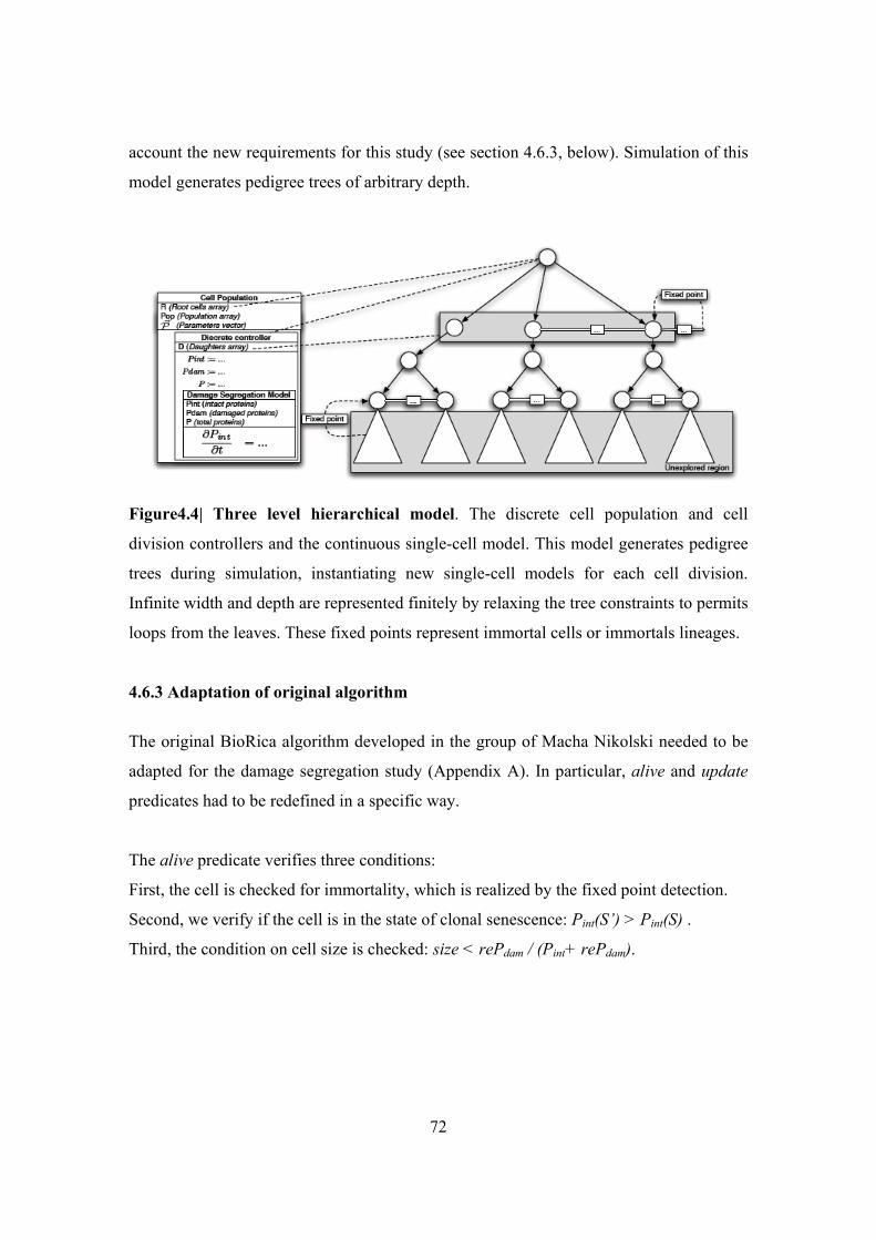
72

account the new requirements for this study (see section 4.6.3, below). Simulation of this

model generates pedigree trees of arbitrary depth.

Figure4.4| Three level hierarchical model. The discrete cell population and cell

division controllers and the continuous single-cell model. This model generates pedigree

trees during simulation, instantiating new single-cell models for each cell division.

Infinite width and depth are represented finitely by relaxing the tree constraints to permits

loops from the leaves. These fixed points represent immortal cells or immortals lineages.

4.6.3 Adaptation of original algorithm

The original BioRica algorithm developed in the group of Macha Nikolski needed to be

adapted for the damage segregation study (Appendix A). In particular, alive and update

predicates had to be redefined in a specific way.

The alive predicate verifies three conditions:

First, the cell is checked for immortality, which is realized by the fixed point detection.

Second, we verify if the cell is in the state of clonal senescence: Pint(S’) > Pint(S) .

Third, the condition on cell size is checked: size < rePdam / (Pint+ rePdam).

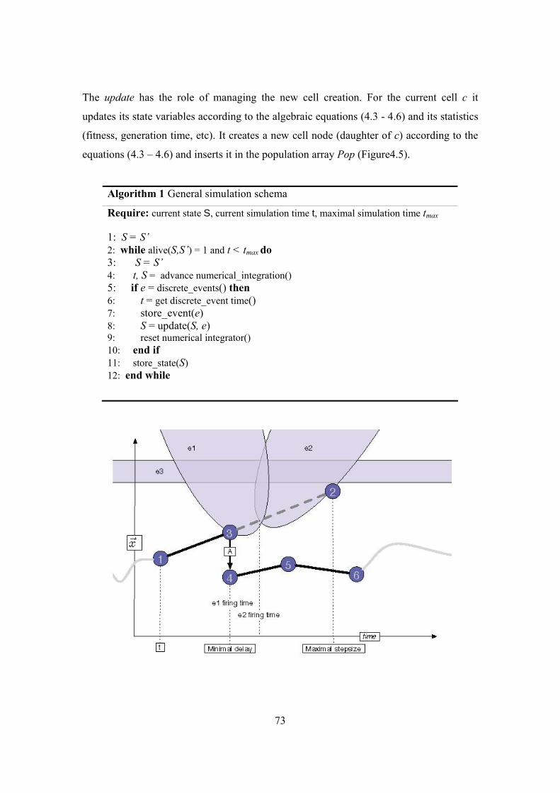
73

The update has the role of managing the new cell creation. For the current cell c it

updates its state variables according to the algebraic equations (4.3 - 4.6) and its statistics

(fitness, generation time, etc). It creates a new cell node (daughter of c) according to the

equations (4.3 – 4.6) and inserts it in the population array Pop (Figure4.5).

Algorithm 1 General simulation schema

Require: current state S, current simulation time t, maximal simulation time tmax 1: S = S’ 2: while alive(S,S’) = 1 and t < tmax do 3: S = S’ 4: t, S = advance numerical_integration() 5: if e = discrete_events() then 6: t = get discrete_event time() 7: store_event(e) 8: S = update(S, e) 9: reset numerical integrator() 10: end if 11: store_state(S) 12: end while

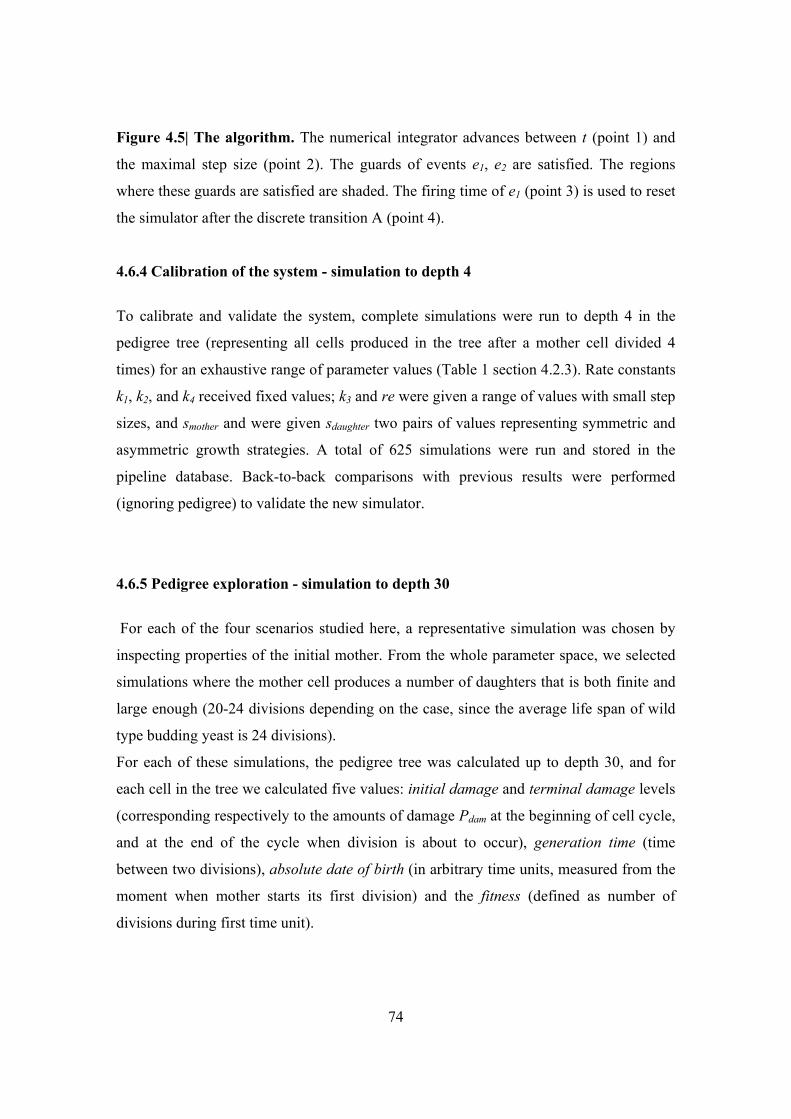
74

Figure 4.5| The algorithm. The numerical integrator advances between t (point 1) and

the maximal step size (point 2). The guards of events e1, e2 are satisfied. The regions

where these guards are satisfied are shaded. The firing time of e1 (point 3) is used to reset

the simulator after the discrete transition A (point 4).

4.6.4 Calibration of the system - simulation to depth 4

To calibrate and validate the system, complete simulations were run to depth 4 in the

pedigree tree (representing all cells produced in the tree after a mother cell divided 4

times) for an exhaustive range of parameter values (Table 1 section 4.2.3). Rate constants

k1, k2, and k4 received fixed values; k3 and re were given a range of values with small step

sizes, and smother and were given sdaughter two pairs of values representing symmetric and

asymmetric growth strategies. A total of 625 simulations were run and stored in the

pipeline database. Back-to-back comparisons with previous results were performed

(ignoring pedigree) to validate the new simulator.

4.6.5 Pedigree exploration - simulation to depth 30

For each of the four scenarios studied here, a representative simulation was chosen by

inspecting properties of the initial mother. From the whole parameter space, we selected

simulations where the mother cell produces a number of daughters that is both finite and

large enough (20-24 divisions depending on the case, since the average life span of wild

type budding yeast is 24 divisions).

For each of these simulations, the pedigree tree was calculated up to depth 30, and for

each cell in the tree we calculated five values: initial damage and terminal damage levels

(corresponding respectively to the amounts of damage Pdam at the beginning of cell cycle,

and at the end of the cycle when division is about to occur), generation time (time

between two divisions), absolute date of birth (in arbitrary time units, measured from the

moment when mother starts its first division) and the fitness (defined as number of

divisions during first time unit).

75

4.7 Rejuvenation Study

Using parameter exploration we could identify sets of parameters that exhibit a given

emerging high-level behavior. Moreover, the analysis of the emerging behavior can be

done both at the single-cell and whole pedigree tree levels.

The model was analyzed for different initial amount of damaged and intact proteins.

Thus, we could compute the critical level of terminal damage (Pdam at the point of

division) to find the set of initial values which would gives us the cells that exhibit death

(Figure 4.6 - left panel).

Pdam(0)

P int(0

)

cell

deat

h

Pdam(0)

cell

deat

h

Pdam at Division Time until next Division

0.00.10.20.30.40.50.60.70.80.91.0

Pdam(0)

P int(0

)

cell

deat

h

Pdam(0)

cell

deat

h

Pdam at Division Time until next Division

0.00.10.20.30.40.50.60.70.80.91.0

Figure 4.6| Variation of initial values of Pint and Pdam and their effect on terminal damage and generation time. Similarly, the time until next division can be calculated as a function of initial values of

intact and damaged proteins (Figure 4.6 - right panel).

However, here we observe the opposite effect of increased initial values of intact

proteins, which lead to have long period of time until cell divides, which would

correspond to long generation time and it is consistent with observations that generation

time becomes progressively longer as mother cells become older.

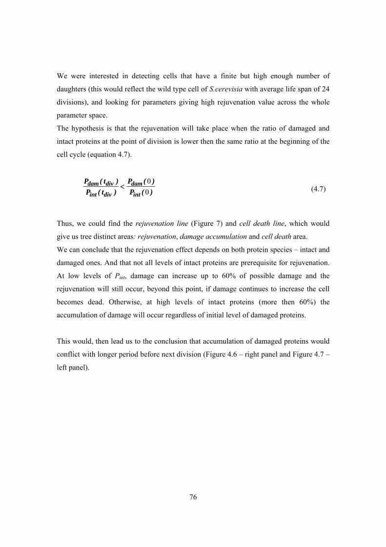
76

We were interested in detecting cells that have a finite but high enough number of

daughters (this would reflect the wild type cell of S.cerevisia with average life span of 24

divisions), and looking for parameters giving high rejuvenation value across the whole

parameter space.

The hypothesis is that the rejuvenation will take place when the ratio of damaged and

intact proteins at the point of division is lower then the same ratio at the beginning of the

cell cycle (equation 4.7).

00

dam div dam

int div int

P ( t ) P ( )P ( t ) P ( )

< (4.7)

Thus, we could find the rejuvenation line (Figure 7) and cell death line, which would

give us tree distinct areas: rejuvenation, damage accumulation and cell death area.

We can conclude that the rejuvenation effect depends on both protein species – intact and

damaged ones. And that not all levels of intact proteins are prerequisite for rejuvenation.

At low levels of Pint, damage can increase up to 60% of possible damage and the

rejuvenation will still occur, beyond this point, if damage continues to increase the cell

becomes dead. Otherwise, at high levels of intact proteins (more then 60%) the

accumulation of damage will occur regardless of initial level of damaged proteins.

This would, then lead us to the conclusion that accumulation of damaged proteins would

conflict with longer period before next division (Figure 4.6 – right panel and Figure 4.7 –

left panel).

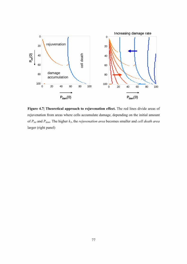
77

0 20 40 60 80 100100

80

60

40

20

0

0 20 40 60 80 100100

80

60

40

20

0

Pdam(0)

P int(0

)

cell

deat

h

rejuvenation

damage accumulation

Pdam(0)

Increasing damage rate

0 20 40 60 80 100100

80

60

40

20

0

0 20 40 60 80 100100

80

60

40

20

0

Pdam(0)

P int(0

)

cell

deat

h

rejuvenation

damage accumulation

Pdam(0)

Increasing damage rate

Figure 4.7| Theoretical approach to rejuvenation effect. The red lines divide areas of

rejuvenation from areas where cells accumulate damage, depending on the initial amount

of Pint and Pdam. The higher k3, the rejuvenation area becomes smaller and cell death area

larger (right panel)

78

4.8 Results

4.8.1 Effects of asymmetry on clonal senescence With the equations at hand, we asked whether there is an intrinsic difference between

symmetrically and asymmetrically dividing systems in their ability to cope with

increasing rates of damage production. The model was simulated initially for low damage

rates with an equal inheritance of damaged proteins (Figure 4.8A). Under these

conditions the system is characterized by constant initial and final concentrations of intact

and damaged proteins during successive generations and the population is immortal

(Figure 4.8A). At moderate damage rates, cells still divide indefinitely but display longer

generation times (Figure 4.8A). In contrast, at high damage rates, the cells go through a

finite number of divisions characterized by progressively longer generation times and a

pronounced accumulation of damaged proteins at the expense of intact ones, eventually

preventing Pdiv from being attained (Figure 4.8A). Since division, in this simulation, is

perfectly symmetrical and all cells in the population are identical, the outcome is clonal

senescence. That is, the model predicts that at high damage rates the entire population

eventually reaches a “dead end”, reminiscent of the Hayflick limit.

We next asked whether a “division of labor”, i.e. the unequal distribution of damaged

proteins during cytokinesis (Figure 4.2B) among individuals affects the damage rate at

which clonal senescence is reached. We therefore introduced the retention coefficient into

the model (see equations (4.6) and (4.7)); such that equal-sized siblings are

distinguishable by the amount of damaged proteins they inherit. The system now shows

signs of sibling-specific replicative senescence, with the cells retaining more of the

damage displaying progressively longer generation times whereas the “low-damage”

sibling lineage propagates indefinitely (Figure 4.8B). In addition, everything else being

equal, damage segregation (Figure 4.8B) allows the population to expand at damage

rates, which cause clonal senescence of a perfectly symmetric system (Figure 4.8A).

79

1500

1000

500

1500

1000

500

1500

1000

500

1500

1000

500

1500

1000

500

1500

1000

500

2500

1500

500

1500

1000

500

1500

1000

500

3000

2000

1000

3000

2000

1000

3000

2000

1000

1500

1000

500

1 2 3 1 2 31 2 3 1 2 3 1 2 3

Time (arbitrary units)

Num

ber o

f mol

ecul

es

No damage retention Damage retention

Dam

age

rate

(K3)

0.6

1.0

1.7

A BSibling-1 Sibling-2 Sibling-1 (mother) Sibling-2 (daughter)

Figure4.8| Symmetrical division.Time course comparison between symmetrically dividing cells without retention and with retention of

damaged proteins and with a low, medium and high degree of damaged proteins being generated. We see that all three protein amounts

P, Pint, Pdam, increase until Pint reaches Pdiv. Then the cells divide and distribute protein amounts according to equations (4.3) and (4.4) in

case of no segregation or equation (4.5) and (4.6) in case of segregation. Mother and daughter cells, in the case of symmetrical division

we would refer to them as sibling-1 and sibling-2 behave identically when division is symmetric and retention not applied (Figure2A);

however, they follow two distinct patterns of protein inheritance, when retention is introduced (Figure 2B).

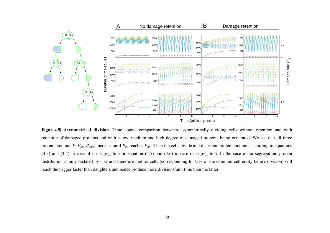
80

1500

1000

500

1500

1000

500

1500

1000

500

1500

1000

500

1500

1000

500

2500

1500

500

1500

1000

500

1500

1000

500

3000

2000

1000

1500

1000

500

3000

2000

1000

1500

1000

500

1 2 3 1 2 31 2 3 1 2 3 1 2 3

Time (arbitrary units)

Num

ber o

f mol

ecul

es

No damage retention Damage retention

Dam

age

rate

(K3)

0.6

1.0

1.7

A B

Figure4.9| Asymmetrical division. Time course comparison between asymmetrically dividing cells without retention and with

retention of damaged proteins and with a low, medium and high degree of damaged proteins being generated. We see that all three

protein amounts P, Pint, Pdam, increase until Pint reaches Pdiv. Then the cells divide and distribute protein amounts according to equations

(4.3) and (4.4) in case of no segregation or equation (4.5) and (4.6) in case of segregation. In the case of no segregation, protein

distribution is only dictated by size and therefore mother cells (corresponding to 75% of the common cell entity before division) will

reach the trigger faster than daughters and hence produce more divisions/unit time than the latter.

81

This analysis was followed by testing whether a difference in size alone between a large

progenitor and a smaller offspring (Figure 4.3A) is sufficient to prevent clonal

senescence. In this context, the inheritance of intact and damaged proteins is proportional

to the relative size of each cell entity at division. At low to moderate damage, the system

now shows signs of a sibling-specific replicative senescence, typical of asymmetrical

dividing systems, such as budding yeast. The larger parent lineage (mother cell) displays

increasingly longer generation times (Figure 4.9A) until eventually the persistent titration

of intact proteins by damaged ones prevents it from dividing again. In contrast, at the

same damage rate, the smaller progeny lineage continues to divide indefinitely (Figure

4.9A). Also, a system of different-sized progeny can expand ad infinitum even without

damage segregation at damage rates giving rise to clonal senescence in the perfectly

symmetrical system (Figure 4.8A and 4.9A). When damage was segregated such that the

larger mother cells received an even higher load than expected from its size (Figure

4.9B), the system could withstand even higher levels of damage before clonal senescence

commenced (Figure 4.9B).

The model also suggests that in order to prevent clonal senescence the degree of damage

segregation (or size asymmetry) needs to increase as the damage production rate is

elevated (Figure 4.10A and B). The trade-off for this beneficial effect of damage

retention or size asymmetry on clonal senescence is sibling-specific aging at

progressively lower damage rates (Figure 4.10A and B). Interestingly, even very low

retention coefficients (re=0.125; one sibling effectively retaining 58% of the overall Pdam)

are sufficient to prevent a symmetrically dividing population from reaching a “dead end”

at moderate damage rates (Figure 4.10A).

82

A

0.5 1.0 1.5 2.0

0.0

0.125

0.250

0.375

0.500

0.650

0.750

0.875

Ret

entio

n

Asy

mm

etry

0.5 1.0 1.5 2.0

Damage production rate

50-50

10-90

40-60

25-75

B

Damage production rate

A

0.5 1.0 1.5 2.0

0.0

0.125

0.250

0.375

0.500

0.650

0.750

0.875

Ret

entio

n

Asy

mm

etry

0.5 1.0 1.5 2.0

Damage production rate

50-50

10-90

40-60

25-75

B

Damage production rate Figure 4.10| Damage segregation and size asymmetry causes sibling-specific aging

but increases the robustness of the system. (A) Effect of damage segregation (y-axis)

on damage levels (k3; x-axis) triggering clonal senescence and replicative aging. Green

bars indicate that both siblings produced during cytokinesis are immortal but exhibit

longer generation times with increasing damage. Red bars indicate that the sibling

retaining more damage at the time of cytokinesis undergoes replicative senescence, i.e.

can only perform a finite number of new generations, whereas the other sibling is

immortal. Empty bars indicate that the system has reached clonal senescence, i.e. a

damage rate at which both siblings display a finite ability to produce new cells. (B) Effect

of size asymmetry (y-axis) on damage levels (k3; x-axis) triggering clonal senescence and

replicative aging. Color-coding is as described in “A”.

83

4.8.1.1 Generation time

The simulations also suggest that the generation time of the damaged-enriched mother

cell increases exponentially with each cell division in the system displaying damage

retention whereas a slow linear increase is observed for mother cells without retention of

damage (Figure4.11A). Again, the experimental data for mother cells of budding yeast

fits best with the simulations of damage retention (Figure4.11B).

A

Gen

erat

ion

time

(arb

itrar

y un

its)

5 10 15 20

0.1

0.8

Age of mother (generations)

180

120

60

1 10 20 30Age of mother

Gen

erat

ion

time

(min

)

BA

Gen

erat

ion

time

(arb

itrar

y un

its)

5 10 15 20

0.1

0.8

Age of mother (generations)

180

120

60

1 10 20 30

180

120

60

1 10 20 30

60

1 10 20 30Age of mother

Gen

erat

ion

time

(min

)

B

Figure4.11| Effect of damage segregation on generation time of the mother-cell

lineage in an asymmetrically dividing system. (A) Changes in generation time (y-axis)

are plotted as a function of age of the large mother cell in an asymmetrically dividing

systems without (red) and with (blue) damage segregation. (B) Experimental data for the

generation time of yeast mother cells as a function of the replicative age.

4.8.1.2 Increase in size

One of the biomarkers for yeast ageing process is increase in size. This is, probably, the

most obvious feature of a senescent cell. Several studies showed that the volume of the

yeast cell increases linearly with age and that the senescent cell can be four times as large

as an exponentially growing cell.

A system obeying the roles of Pdiv and damage propagation as stipulated in the equations

requires that the mother cell becomes progressively larger with each division, which is

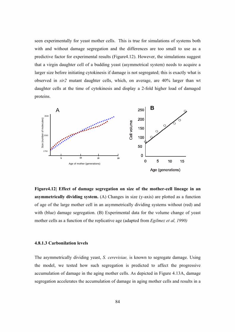
84

seen experimentally for yeast mother cells. This is true for simulations of systems both

with and without damage segregation and the differences are too small to use as a

predictive factor for experimental results (Figure4.12). However, the simulations suggest

that a virgin daughter cell of a budding yeast (asymmetrical system) needs to acquire a

larger size before initiating cytokinesis if damage is not segregated; this is exactly what is

observed in sir2 mutant daughter cells, which, on average, are 40% larger than wt

daughter cells at the time of cytokinesis and display a 2-fold higher load of damaged

proteins.

5 10 15 205 10 15 20

Age of mother (generations)

1750

2350

3500

Size

(num

ber o

f mol

ecul

es)

A B

Figure4.12| Effect of damage segregation on size of the mother-cell lineage in an

asymmetrically dividing system. (A) Changes in size (y-axis) are plotted as a function

of age of the large mother cell in an asymmetrically dividing systems without (red) and

with (blue) damage segregation. (B) Experimental data for the volume change of yeast

mother cells as a function of the replicative age (adapted from Egilmez et al, 1990)

4.8.1.3 Carbonilation levels

The asymmetrically dividing yeast, S. cerevisiae, is known to segregate damage. Using

the model, we tested how such segregation is predicted to affect the progressive

accumulation of damage in the aging mother cells. As depicted in Figure 4.13A, damage

segregation accelerates the accumulation of damage in aging mother cells and results in a

85

differential accumulation of damage during the cell cycle – mother cells that retain

damage have longer generation times and the number of damaged molecules (per total) is

somewhat decreasing during the cell cycle (Figure 4.13A). In contrast, mother cells that

do not retain damage exhibit more even levels of damage throughout the cell cycle and

do not display the step-wise increase in damage upon cytokinesis observed in damage-

retaining mother cells (Figure 4.13A). We measured the concentration of oxidatively

damage proteins (per total) in synchronized yeast mother cells during two successive

divisions and noted that the damage displays a step-wise increase in the mother cell upon

completion of cytokinesis (Figure 4.13B).

0.1

0.2

0.3

0.4

0.5

0.2 0.4 0.6 0.8

P dam

/Pto

t

Time (arbitrary units)

A

100 200

0.8

0.6

0.4

Time

Pda

m/P

tot

B

0.1

0.2

0.3

0.4

0.5

0.2 0.4 0.6 0.8

P dam

/Pto

t

Time (arbitrary units)

A

100 200

0.8

0.6

0.4

100 200

0.8

0.6

0.4

0.8

0.6

0.4

Time

Pda

m/P

tot

B

Figure4.13| Effect of damage segregation on damage accumulation of the mother-

cell lineage in an asymmetrically dividing system. (A) The ratio of damaged to total

number of molecules (y-axes) in the large mother cells during progressive cell cycles in

an asymmetrically dividing system without (red) and with (blue) damage segregation. In

the system without retention, the large mother cells accomplish 7 divisions and the

system with retention 4 divisions during the time shown. (B) Experimental data for the

ratio of oxidized to total proteins during two successive cell cycles of yeast mother cells:

an asymmetrical system known to segregate damaged proteins.

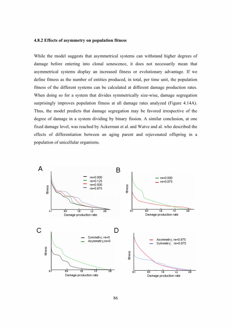
86

4.8.2 Effects of asymmetry on population fitness

While the model suggests that asymmetrical systems can withstand higher degrees of

damage before entering into clonal senescence, it does not necessarily mean that

asymmetrical systems display an increased fitness or evolutionary advantage. If we

define fitness as the number of entities produced, in total, per time unit, the population

fitness of the different systems can be calculated at different damage production rates.

When doing so for a system that divides symmetrically size-wise, damage segregation

surprisingly improves population fitness at all damage rates analyzed (Figure 4.14A).

Thus, the model predicts that damage segregation may be favored irrespective of the

degree of damage in a system dividing by binary fission. A similar conclusion, at one

fixed damage level, was reached by Ackerman et al. and Watve and al. who described the

effects of differentiation between an aging parent and rejuvenated offspring in a

population of unicellular organisms.

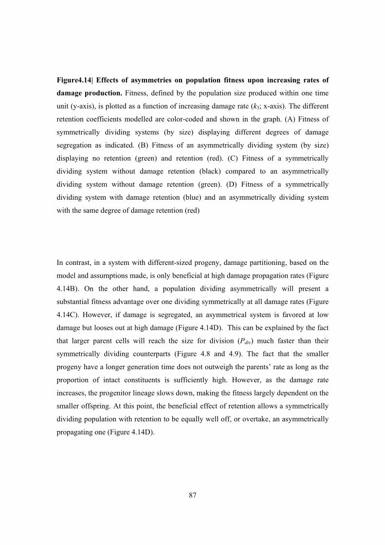
87

Figure4.14| Effects of asymmetries on population fitness upon increasing rates of

damage production. Fitness, defined by the population size produced within one time

unit (y-axis), is plotted as a function of increasing damage rate (k3; x-axis). The different

retention coefficients modelled are color-coded and shown in the graph. (A) Fitness of

symmetrically dividing systems (by size) displaying different degrees of damage

segregation as indicated. (B) Fitness of an asymmetrically dividing system (by size)

displaying no retention (green) and retention (red). (C) Fitness of a symmetrically

dividing system without damage retention (black) compared to an asymmetrically

dividing system without damage retention (green). (D) Fitness of a symmetrically

dividing system with damage retention (blue) and an asymmetrically dividing system

with the same degree of damage retention (red)

In contrast, in a system with different-sized progeny, damage partitioning, based on the

model and assumptions made, is only beneficial at high damage propagation rates (Figure

4.14B). On the other hand, a population dividing asymmetrically will present a

substantial fitness advantage over one dividing symmetrically at all damage rates (Figure

4.14C). However, if damage is segregated, an asymmetrical system is favored at low

damage but looses out at high damage (Figure 4.14D). This can be explained by the fact

that larger parent cells will reach the size for division (Pdiv) much faster than their

symmetrically dividing counterparts (Figure 4.8 and 4.9). The fact that the smaller

progeny have a longer generation time does not outweigh the parents’ rate as long as the

proportion of intact constituents is sufficiently high. However, as the damage rate

increases, the progenitor lineage slows down, making the fitness largely dependent on the

smaller offspring. At this point, the beneficial effect of retention allows a symmetrically

dividing population with retention to be equally well off, or overtake, an asymmetrically

propagating one (Figure 4.14D).

88

4.8.3 Damage segregation in a system dividing by binary fission Segregation of damage has, so far, only been demonstrated for the asymmetrically

dividing budding yeast. The fact that our simulations suggest that a system dividing

symmetrically by size is more robust (withstand more damage before reaching clonal

senescence) and displays an increased fitness at all damage propagation rates when

partitioning its damage during cytokinesis raises the possibility that damage segregation

is more common than previously anticipated and occurs also in cells dividing by binary

fission. This prompted us to analyze the in situ distribution of carbonylated proteins in

the fission yeast, Schizosaccharomyces pombe.

While the volume of the two siblings is equal, previous landmarks of division (birth

scars), will remain confined to one half of the growing cell and be inherited by one “sib”

only (Figure 4.15). When following birth scars and protein carbonyls during the cell cycle

in synchronized cells, we found that carbonylated proteins display a discrete and dynamic

localization within the cell (Figure 4.16). Quantification of carbonyls demonstrated that

damage is inherited asymmetrically between the two siblings such that the one with the

previous birth scar always retains the largest load of the damage (Figure 4.16). After

completion of cytokinesis, the newborn cells display most of their damage at the new end

(Figure4.16).

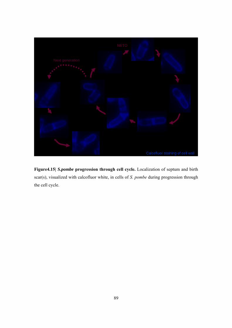
89

Next generation

NETO

Calcofluor staining of cell wall

Figure4.15| S.pombe progression through cell cycle. Localization of septum and birth

scar(s), visualized with calcofluor white, in cells of S. pombe during progression through

the cell cycle.

90

Next generation

NETO

New/Old

New/Old

New/Old In situ carbonylation

Figure4.16| Damaged proteins are asymmetrically segregated during binary fission

of S. pombe. Distribution of carbonylated proteins during the cell cycle. Blue/purple

denotes the highest concentration of carbonyls followed by red and yellow.

We next investigated whether partitioning of damaged proteins between the two siblings

correlated with differential fitness or longevity. We followed the replicative potential of

both sibling lineages, arising from division of a common parent cell, which had already

completed 9 divisions and thus accumulated damaged proteins (see Figure 4.17A). We

found that the sibling enriched for birth scars and protein damage (“old” sib) displayed a

shorter mean life span (12.5 generations) than the “young” sib (15.9 generations)(Figure

4.17B), Moreover, the generation time of the damage enriched cell was markedly longer

– 4.5 hours compared to 2.5 hours for the new sib (Figure 4.17C). This result points to a

“sibling-specific” aging in S. pombe that correlates with the unequal inheritance of

damaged proteins.

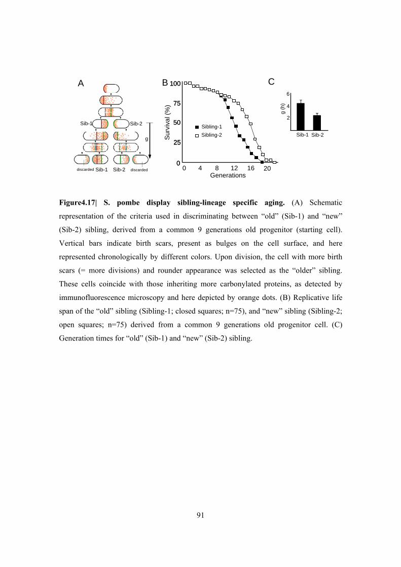
91

gf g

ih

Sibling-1Sibling-2

4 8 12 16 200

100

75

50

25

0

100

75

50

25

0Su

rvi v

a l ( %

)Generations

Sib-2Sib-1g

discarded Sib-1 Sib-2

Sib-2Sib-1

discarded

A B C

g (h

)

2

4

6

Figure4.17| S. pombe display sibling-lineage specific aging. (A) Schematic

representation of the criteria used in discriminating between “old” (Sib-1) and “new”

(Sib-2) sibling, derived from a common 9 generations old progenitor (starting cell).

Vertical bars indicate birth scars, present as bulges on the cell surface, and here

represented chronologically by different colors. Upon division, the cell with more birth

scars (= more divisions) and rounder appearance was selected as the “older” sibling.

These cells coincide with those inheriting more carbonylated proteins, as detected by

immunofluorescence microscopy and here depicted by orange dots. (B) Replicative life

span of the “old” sibling (Sibling-1; closed squares; n=75), and “new” sibling (Sibling-2;

open squares; n=75) derived from a common 9 generations old progenitor cell. (C)

Generation times for “old” (Sib-1) and “new” (Sib-2) sibling.

92

4.8.4 Pedigree analysis In the pedigree tree, a given mother cell generates a series of daughter cells: these

siblings are ordered in time and the younger a sibling, the older the mother at the time of

division. (Figure 4.18)

Daughter numberPdam initalGeneration timePdam terminal

Apsolut time of birthGeneration number

Cell id

#daughters/1time unit

Figure4.18| Extract of typical pedigree tree. Full tree is in Appendix A, section A.4.

In the pedigree tree, the root represents the mother cell with following information:

Daughter number – daughter reproduced by the root cell, Pdam initial – amount of

damaged proteins at the beginning of the cell cycle for given daughter, Generation time –

the length of the cell cycle for given daughter, Pdam terminal - amount of damaged

proteins at the end of the cell cycle for given daughter, Absolute time of birth –

cumulative time of birth counted from the fist daughter produced, Generation number –

depth of the tree developed for specific mother The second level of the tree represents

grand daughters of root mother, third level are grand-grand daughters, and so one.

93

Analyzing the pedigree trees obtained from BioRica simulator can be hard since the

generated trees are usually very large and overwhelmed with all kinds of information, we

can extract data of interest for specific phenomena and generate simplified trees.

Example of such a tree, made for capturing the behavior of damaged proteins at the point

of cell division (end of cell cycle) for a successive daughter cells is shown below (Figure

4.19).

Figure 4.19| Simplified pedigree tree. The mother – daughter relationship is presented,

showing only fitness and terminal damage amount. m- mother, di – ith daughter, mdi - ith

daughter becoming the mother, ddi – ith daughters daughter, dmdi – ith daughter of mother

obtained from ith daughter.

94

We observe in simulation results that younger siblings have higher damage, consistent

with inheritance from an older mother that has accumulated more damaged proteins, and

these younger siblings are thus born “prematurely old.” This increase in damage

accumulation is reflected in the decrease of fitness values (Figure 4.19).

4.8.5 Rejuvenation

Extending analysis of the pedigree tree, one level further, we can obtain grand-daughters

cell line (second generation). We observed that daughters born early to the same mother

have low damage, and their daughters have normal fitness. Daughters born late to the

same mother have high damage and lower fitness, but remarkably, in asymmetric division

with or without retention, their own daughters are born with lower damage and higher

fitness (Figure 4.20 and 4.21)

This increase in fitness in the second generation is a rejuvenation effect, in part

explaining how populations maintain viability over time despite inheritance of protein

damage. The testable hypothesis is thus that there exists a mechanism for retention of

damaged proteins during cell division, that attenuates the accumulation of such proteins

in descendants, and that a combination of the precise value of the corresponding retention

coefficient (re) and the asymmetry coefficients (smother and sdaughter) in the model

determines the scale of the rejuvenation effect. These predictions are consistent with in

vivo experimental results reported in the literature: Kennedy (1994) reported that

daughter cells of an old mother cell are born prematurely old, with lower replicative

potential, but that the daughters of these daughters have normal life spans. It should

therefore be possible to experimentally estimate the value of the retention coefficient

through indirect measures of cell lifespan and replicative potential.

As a control, we also inspected the case of symmetric division without damage

segregation (Figure 4.22). We would not expect a rejuvenation effect, since inheritance of

damaged proteins should be proportional in both mother and daughter cells, and indeed

this is what is observed.

95

Figure 4.20| Asymmetrical division without retention. Mother cell is represented in the

root of the tree, in the second level all her daughters are given (this particular mother

produces 25 daughters before dying). In the third level, daughters produced by daughter 1

and daughter 24 are presented. Fitness is calculated as the number of cells produced per

time unit. In the second level the fitness decreases as mother’s age increases. The

rejuvenation effect is seen in the third level of the tree, where the first daughter produced

from 24th daughter (in the second level) has increased fitness.

96

Figure 4.21|Asymmetrical division with retention. Mother cell is represented in the

root of the tree, in the second level all her daughters are given (this particular mother

produces 20 daughters before dying). In the third level, daughters produced by daughter 1

and daughter 19 are presented. Fitness is calculated as the number of cells produced per

time unit. In the second level the fitness decreases as mother’s age increases. The

rejuvenation effect is seen in the third level of the tree, where the first daughter produced

from 19th daughter (in the second level) has increased fitness.

97

Figure4.22| Symmetrical division without retention. Mother cell is represented in the

root of the tree, in the second level all her daughters are given (this particular mother

produces 20 daughters before dying). In the third level, daughters produced by daughter 1

and daughter 18 are presented. Fitness is calculated as the number of cells produced per

time unit. In the second level the fitness decreases as mother’s age increases. Since the

division is perfectly symmetrical rejuvenation effect, as expected, is not observed.

98

4.8.6 Sensitivity Analysis

Division threshold (Pdiv) – the amount of intact proteins that cell has to attain before

division, can in theoretical approach mimic the various cell sizes critical for division.

This can be used to simulate different mutants whose size is either smaller or larger then

in the wild-type cells. Keeping all the parameters as before, we can decrease Pdiv as low

as 1 molecule, and increase it up to 3500 molecules (at this threshold the system will not

divide – we call this maximum size of the cell). As the level of Pdiv is decreasing, the

number of divisions per one unit time will exponentially increase for all cells regardless

of the division type. And, as we increase Pdiv, the number of division per one time unit

will exponentially decrease. To verify the robustness of the system, the population size

was obtained for both types of division, without retention and with retention (re=0.875).

The results are showing the same trend and behavior as for the Pdiv=1500. The only

difference is that the bigger the Pdiv, the lower damage system can handle (maximum

damage is k3=1.2).

Increasing the rate of degradation of damaged proteins (k4), such that k2 < k4, we will get

daughters that will never reach clonal senescence, while their mothers will be able to

cope with higher damage (k3). Higher rate of degradation for intact proteins (k2 > k4) will

affect fitness of mothers and daughters and their capability of handling higher damage

rates. Both, mothers and daughters will reach clonal senescence much earlier (k3=0.7).

Finally, in simulations we observe that fitness and viability are sensitive to precise values

of k3, the rate by which proteins are damaged. This provides a series of testable

hypotheses that could be investigated experimentally in different damaging

environments, such as oxidative damage or radiation damage.

99

5 Discussion Despite the large number of experimental data, the full understanding of complex ageing

process is still unknown. The natural way would lead to development of mathematical

models which would serve as a platform for better understanding of produced data, would

allow integration of diverse information and postulate untested scenarios. With the

instruments developed in the field of systems biology, tackling such issues become more

feasible and realistic.

This work represents the first dynamic ageing model and further more a model applicable

to different species. Previous models were mainly stochastic (formation of ERCs

developed by Gillespie, bacterial ageing model developed by Ackermann) or more

general and very descriptive and not suitable for direct experimental comparison

(disposable soma model and MARS model, both developed by Tom Kirkwood).

In the this work we approached the questions of whether there is an advantage to

producing daughter cells of different size, different loads of damage, and unequal

reproductive potential. We investigated the impact of damage accumulation on

population robustness and fitness and tested different strategies through which the effects

of damage can be ameliorated. The models predicts that in a growing system adhering to

the rules and assumptions made, there is a maximum amount of damage the cell system

can tolerate, beyond which the proportion of intact constituents becomes insufficient for

the cell to carry out any further division. In a completely homogeneous population, this

point is marked by the simultaneous death (growth-arrest) of all individuals, i.e. clonal

senescence (Figure 4.2A). The entities of the population could, of course, avoid such

clonal senescence by reducing the rate of conversion of intact proteins to damaged ones

(k3) or increasing the rate of damage protein removal (k4), i.e. by increasing their

investment in classical maintenance pathways. However, the simulations suggest that

there are other means of “rescuing” a cell population having reached clonal senescence,

mainly by diversifying individuals within the population. This can be achieved either by

100

unequal partitioning of damage during cytokinesis or producing progeny of different size.

In either case, this diversification of individuals leads to lineage-specific aging. This is in

line with views of Partridge and Barton (1993) and Kirkwood (1981), who considered

potential benefits of asymmetry in simple unicellular systems and how this might develop

into aging.

The uneven distribution of damaged proteins may seem intuitive for organisms

displaying markedly asymmetrical cytokinesis such as budding yeast; less so when there

is no apparent distinction between the two sister cells. However, Stewart and colleagues

demonstrated that Escherichia coli cells enriched with old pole material displayed a

longer generation time than their new pole enriched siblings, indicating asymmetries also

in systems dividing by binary fission. Although the measured differences in generation

times are small in absolute terms, such asymmetry may be of significance for the

robustness and fitness of the population. Our model suggests that even very low

retention coefficients, e.g. a scenario where one cell receives 58% and the other 42% of

the damage, may have a great impact on the systems ability to escape clonal senescence,

at least at moderate damage rates (Figure 4.10). As the damage rate increases, the damage

retention, or size asymmetry, needs to be more pronounced to allow the survival of the

population.

However, when the total fitness (number of cells produced per time unit) of the systems

is considered, damage retention may be a mixed blessing; for example, when considering

a different cell-size organism like budding yeast, damage retention will push the upper

limits for how much damage the system can endure before entering clonal senescence

(Figure 4.10) but become a selective disadvantage at low damage production rates

(Figure 4.14). This raises the question of whether the efficiency of damage segregation

could be adjusted with changing environmental demands. Interestingly, damage

segregation in budding yeast becomes more pronounced following increased oxidative

stress, suggesting that this unicellular organism, indeed, enjoys the capacity to increase

damage segregation upon conditions elevating such damage. In addition, unusually

difficult growth conditions elicit a switch from a morphologically symmetrical to a more

101

asymmetrical type of division in fission yeast indicating that also this organism display a

dynamic ability to break up symmetry upon environmental demands.

One common assumption in reports modeling potential benefits of asymmetry is that the

establishment of age asymmetry is linked to damage segregation. However, such

segregation of damage has, as far as we know, only been shown in the asymmetrically

dividing budding yeast and one of the somewhat surprising predictions of the model

presented here is that a system dividing symmetrically by size (binary fission) display a

higher fitness if damage is segregated regardless of the damage accumulation rate. This

suggests that damage retention may be more common than previously anticipated and

prompted us to analyze the distribution of oxidatively carbonylated proteins during

cytokinesis in the fission yeast S. pombe. We show that S.pombe displays an uneven

distribution of carbonylated proteins between siblings, which correlates with their

longevity and fitness (Figure 4.15, 4.16 and 4.17). This result can explain why growth in

the presence of minor stressors results in a higher mortality of the “sibs” with more birth

scars, i.e. the ones shown here to inherit more damage. Even though partitioning of

damaged proteins to the “older” sib is not as pronounced as that of the budding yeast, it

appears to be sufficient to entrust the “younger” sib with a significantly longer replicative

potential and shorter generation time (Figure 4.17). As stated above, our modeling

approach predicts exactly this, i.e. that a small bias towards damage asymmetry has

profound consequences on the population’s fitness and propagation. Our experimental

results suggest that damage asymmetry is a purely random and stochastic phenomenon.

In addition, the inheritance of the major load of carbonylated proteins is always

coincident with the cell displaying more birth scars.

In summary, within the constrains of the equations and the assumptions made, the data

suggests that both damage and size asymmetries pushes the upper limit for how much

damage a self-propagating unicellular system can tolerate before entering clonal

senescence. We believe the data raises the possibility that sibling-specific aging and

rejuvenation in unicellular systems may have evolved as by-products of a strong selection

for damage segregation during cytokinesis. A question of interest is whether such

102

division of labor between cells undergoing division is retained also in multicellular

organisms, for example during the generation of germ line cells or differentiation.

This thesis showed that computational modeling poses considerable challenges at both

theoretical and experimental levels. The model we developed is yet simple, but fully

predictive, which, as stated at the beginning of this work, is the main feature a model

should have. As a first step ageing model confirmed the findings of well studied model

organism – S.cerevisiae (changes in size, generation time and damage load), then showed

the importance of having damage segregation mechanism to ensure the immortal

population. Finally, the model predicted the damage segregation on symmetrically

dividing system – S.pombe, which was not previously anticipated. This led us to

conclusion that asymmetrical damage distribution is one of the key factors in ageing

organism and that immortal populations are not specific to size-wise asymmetrically

dividing systems.

.

103

References

http://www.sanger.ac.uk/PostGenomics/S_pombe/docs/nurse_lab_manual.pdf

http://www.sbml.org

http://www.wolfram.com/

http://www.r-project.org/

http://www.perl.com/

http://www.yeastgenome.org/

Abrams PA, Ludwig D (1995) Optimality Theory, Gompertz' Law, and the Disposable

Soma Theory of Senescence, Evolution, Vol. 49, No. 6, pp. 1055-1066

Ackerman M, Chao L, Bergstrom CT, Doebeli M (2007) On the evolutionary origin of

aging. Aging Cell 6, 235-244

Ackermann M, Stearns SC, Jenal, U (2003) Senescence in a bacterium with asymmetric

division. Science 300, 1920.

Aguilaniu H, Gustafsson L, Rigoulet M, Nyström T (2003) Asymmetric inheritance of

oxidatively damaged proteins during cytokinesis. Science 299, 1751-1753.

Antal T et al., (2007) Aging and immortality in a cell proliferation model, Journal of

Theoretical Biology 248, 411–417

Austad SN (1997) Why We Age. New York: John Wiley and Sons

Austriaco NR. (1996) Review: to bud until death: the genetics of ageing in the yeast

Saccharomyces. Yeast 12: 623-630

Barker MG, Walmsley RM. (1999) Replicative ageing in the fission yeast

Schizosaccharomyces pombe. Yeast. 15:1511–1518

104

Beckman, KB, Ames, BN (1998) The free radical theory of aging matures. Physiol. Rev.

78, 547-581.

Bitterman KJ, Medvedik O, Sinclair DA. (2003)Longevity regulation in Saccharomyces

cerevisiae: linking metabolism, genome stability, and heterochromatin. Microbiol. Mol.

Biol. Rev.67:376–399

Bruggeman FJ, Westerhoff HV (2007) The nature of systems biology, Trends Microbiol

15, pp. 45–50

Cacuci, DG, Ionescu-Bujor M, Navon M, (2005) Sensitivity And Uncertainty Analysis:

Applications to Large-Scale Systems (Volume II), Chapman & Hall.

Chakravarti B, Chakravarti D (2007) Oxidative Modification of Proteins: Age-Related

Changes, Gerontology,53:128-139

Drenos F, Kirkwood TBL (2005) Modelling the disposable soma theory of ageing.

Mechanisms of Ageing and Development, 126, 99-103.

Egilmez NK, Jazwinski SH (1989) Evidence for the involvement of a cytoplasmic factor

in the aging of the yeast Saccharomyces cerevisiae. J Bacteriol 171: 37−42

Egilmez NK, Chen JB, Jazwinski SM (1990) Preparation and partial characterization of

old yeast cells. J Gerontology 45:B9-B17

Elliott SG, McLaughlin CS (1978) Rate of macromolecular synthesis through the cell

cycle of the yeast Saccharomyces cerevisiae. Proc. Natl. Acad. Sci. USA 75, 4384-4388.

Erjavec N (2007) Divide et impera: damage segregation and rejuvenation in yeast, PhD

thesis, Göteborg University, Sweden

Erjavec N, Nyström T (2007) Sir2p-dependent protein segregation gives rise to a superior

reactive oxygen species management in the progeny of Saccharomyces cerevisiae. Proc.

Natl. Acad. Sci. USA 104, 10877-10881.

Erjavec N, Nyström T (2007) Sir2p-dependent protein segregation gives rise to a superior

reactive oxygen species management in the progeny of Saccharomyces cerevisiae. Proc.

Natl. Acad. Sci. USA 104, 10877-10881.

105

Evans S, Steinsaltz D (2007) Damage segregation at fissioning may increase growth

rates: A superprocess model, Theoretical Population BiologyVolume 71, Issue 4, pp.473-

490

Fabrizio P, Longo VD (2003) The chronological life span of Saccharomyces cerevisiae.

Aging Cell. 2:73–81

Fantes PA (1982) Dependency relations between events in mitosis in

Schizosaccharomyces pombe. J. Cell Sci. 55, 383-402.

Farout L, Friguet B, Proteasome (2006) Function in Ageing and oxidative stress:

implication in protein maintenance failure, Antioxidants & Redox Signaling. 8(1-2): 205-

216. doi:10.1089/ars.2006.8.205

Freeman-Cook LL. et al. (2005) Conserved locus-specific silencing functions of

Schizosaccharomyces pombe sir2+. Genetics 169, 1243-1260.

Friguet B, Bulteau A-L, Chondrogianni N, Conconi M, Petropoulos I, (2000) Protein

Degradation bt the proteasome and its implication in ageing, Annals of the New York

Academy of Sciences, 908:143-154

Gavrilov LA, Gavrilova NS (2001) The reliability theory of aging and longevity, J.

Theor. Biol. 213, pp. 527–545

Gillespie CS, Proctor CJ, Boys RJ, Shanley DP, Wilkinson DJ, Kirkwood TB, (2004) A

mathematical model of ageing in yeast, J. Theor. Biol. 229, pp. 189–196

Gillespie DT (1976) A General Method for Numerically Simulating the Stochastic Time

Evolution of Coupled Chemical Reactions, Journal of Computational Physics 22(4), 403-

434

Gillespie DT (1977) Exact Stochastic Simulation of Coupled Chemical Reactions, The

Journal of Physical Chemistry, Vol. 81, No. 25, pp. 2340-2361

Gillespie JH (1974) Natural selection for within-generation variance in offspring number,

Genetics 76, pp. 601–606

106

Glynn JM, Lustig RJ, Berlin A, Chang F. (2001) Role of bud6p and tea1p in the

interaction between actin and microtubules for the establishment of cell polarity in fission

yeast. Curr Biol. 11(11):836-45

Grune, T, Jung, T, Merker, K, Davies, KJA (2004) Decreased proteolysis caused by

protein aggregates, inclusion bodies, plaques, lipofuscin, ceroid, and 'aggresomes' during

oxidative stress, aging, and disease. Int. J. Biochem. Cell Biol. 36, 2519-2530.

Guarente L (2000) Sir2 links chromatin silencing, metabolism, and aging. Genes Dev. 14,

1021-1026.

Hamilton W D (1966) The moulding of senescence by natural selection. J. Theor. Biol.

12:12-45

Harman D (1981) The aging process. In: Proc. Natl. Acad. Sci. USA 78, pp. 7124–7128.

Hayflick L, Moorhead P (1961) The serial cultivation of human diploid cell strains. Exp.

Cell Res. 25, 585-621.

Hernebring M, Brolen G, Aguilaniu H, Semb H, Nyström T (2006) Elimination of

damaged proteins during differentiation of embryonic stem cells. Proc. Nat. Acad. Sci.

USA 103, 7700-7705.

Holliday R. and Kirkwood, TBL (1981) Predictions of the somatic mutation and

mortalization theories of cellular ageing are contrary to experimental observations. J.

Theor. Biol. 93, pp. 627–642

Holliday, R (1975) Growth and death of diploid and transformed human fibroblasts. Fed.

Proc 34, 51-55

Horvitz HR, Herskowitz (1992) Mechanisms of asymmetric cell division: two Bs or not

two Bs, that is the question, Cell 68, pp. 237–255

Huang Y (2002) Transciptional silencing in Saccharomyces cerevisiae and

Schizosaccharomyces pombe. Nucl. Acids Res. 30, 1465-1482.

Kaeberlein M, Powers RW, Steffen KK, Westman EA, Hu D, Dang N, Kerr EO,

Kirkland KT, Fields S, et al. (2005) Regulation of yeast replicative life span by TOR and

Sch9 in response to nutrients. Science, 310:1193–1196

107

Kaeberlein, M.;Burtner, C.; Kennedy, BK (2007) Recent developments in aging. PloS

Genet. doi: 10.1371/journal.pgen.0030084.

Kauffman SA (1969) Metabolic stability and epigenesis in randomly constructed genetic

nets. Journal of Theoretical Biology, 22:437-467

Kauffman SA (1993) Origins of Order: Self-Organization and Selection in Evolution

Oxford University Press.

Kennedy BK, Austriaco JrNR, Guarente L (1994) Daughter cells of Saccharomyces

cerevisiae from old mothers displays a reduced life span. J. Cell Biol. 127, 1985-1993.

Kirkwood T (1981) Repair and its Evolution: Survival versus Reproduction, Chapter 7.

Physiological Ecology: An Evolutionary Approach to Resource Use, Blackwell Scientific

Publications, Oxford.

Kirkwood TB (2005) Understanding the odd science of aging. Cell 120: 437–447

Kirkwood TBL (1977) Evolution of ageing. Nature 270, 301–304

Kirkwood TBL (1989). DNA, mutations and aging. Mutat. Res. 219, pp. 1–7

Kirkwood TBL (1999) Time of our Lives: The Science of Human Ageing. London:

Weidenfeld and Nicolson.

Kirkwood TBL, Franceschi C (1992) Is aging as complex as it would appear? Ann.

NYAcad. Sci. 663, pp. 412–417

Kirkwood TBL, Holliday R (1979) The evolution of ageing and longevity. In: Proc. R.

Soc. Lond., Ser. B 205, pp. 531–546

Kirkwood TBL, Rose MR (1991) ‘‘Evolution of Senescence: Late Survival Sacrificed for

Reproduction.’’ Philosophical Transactions of the Royal Society of London B332 15–24.

Kitano H (2002) Computational Systems Biology Nature. 420, 206-210

Kitano H (2002) Standards for modeling Nat. Biotech. 20, 337

108

Kitano H (2002) Systems Biology: A Brief Overview. Science. 295, 1662-1664

Kitano H (2007) Towards a theory of biological robustness, Mol Syst Biol 3, pp. 1–7

Klipp E, Herwig R., Kowald A., Wierling C and Lehrach H (2005) Systems Biology in

Practice: Concepts, Implementation and Application. Wiley-VCH, Weinheim

Klipp E, Liebermeister W, Helbig A, Kowald A & Schaber J. (2007) Systems Biology

standards – the community speaks. Nature Biotechnology, 25(4), 390-391

Kowald A, Kirkwood TBL (1993) Mitochondrial mutations, cellular instability and

ageing: Modeling the population dynamics of mitochondria. Mutat. Res. 295, pp. 93–103

Kowald A, Kirkwood TBL (1994) Towards a network theory of ageing: A model

combining the free radical theory and the protein error theory. J. Theor. Biol. 168, pp.

75–94

Kowald A, Kirkwood TBL (1996) A network theory of ageing: the interactions of

defective mitochondria, aberrant proteins, free radicals and scavengers in the ageing

process. Mutat. Res. 316, pp. 209–236

Kowald A, Kirkwood TBL (1997) Network theory of ageing, Experimental Gerontology

Volume 32, Issues 4-5, pp. 395-399

Le Novère, N. et al (2005) Minimum information requested in the annotation of

biochemical models (MIRIAM). Nature Biotechnology 23:1509-1515

Leupold U (1970) Genetical methods for Schizosaccharomyces pombe. Methods Cell

Physiol. 4, 169-177.

Levine RL (2002) Carbonyl modified proteins in cellular regulation, aging, and disease.

Free Radic Biol Med 32: 790−796

109

Lin SJ, Kaeberlein M, Andalis AA, Sturtz LA, Defossez PA, Culotta VC, Fink GR,

Guarente L. (2002) Calorie restriction extends Saccharomyces cerevisiae lifespan by

increasing respiration. Nature, 418:344–348

Lindner AB, Madden R, Demarez A, Stewart EJ, Taddei F (2008) Asymmetric

segregation of protein aggregates is associated with cellular aging and rejuvenation Proc.

Natl. Acad. Sci. USA 105, 3076 – 3081

Mangel M (2001) Complex adaptive systems, aging and longevity, J. Theor. Biol. 213,

pp. 559–571.

Martin SG, Chang F. (2005) New end take off, regulating cell polarity during the fission

yeast cell cycle. Cell Cycle 4, 1046-1049.

Mata J, Nurse P (1997) Tea1 and the microtubular cytoskeleton are important for

generating global special order within the fission yeast cell. Cell 89, 939-949.

McMurray MA, Gottschling DE (2003). An age-induced switch to a hyper-

recombinatorial state. Science 301, 1908-1911.

McRae et al., 1982. Global sensitivity analysis-a computational implementation of the

Fourier amplitude sensitivity test (FAST). Comput. Chem. Eng. v6. 15-25.

Medawar P (1957) An unsolved problem in biology. In: The Uniqueness of the

Individual. Basic Books, pp. 1–27

Medvedev, ZA (1981) On the immortality of the germ cell line. Int J Dev Biol, 42, 1037-

1042.

Mitchison JM, Nurse P (1985) Growth in cell length in the fission yeast

Schizosaccharomyces pombe. J. Cell Sci. 75, 357-376.

Mortimer R, Johnston J (1959) Lifespan of Individual Yeast Cells. Nature 183:1751-1752

110

Nasim A, Young P, Johnson BF (1989) Molecular biology of the fission yeast. Academic

Press, New York, NY

Nyström T (2002) Translational fidelity, protein oxidation, and senescence: lessons from

bacteria. Aging Res Rev 1: 693−703

Nyström T. (2005) Role of oxidative carbonylation in protein quality control and

senescence. EMBO J. 24:1311–131

Nyström, T (2007) A Bacterial Kind of Aging. PLoS Genet 3(12): e224

Orgel LE (1963) The maintenance of the accuracy of protein synthesis and its relevance

to ageing. In: Proc. Natl. Acad. Sci. USA 49, pp. 517–521

Partridge L, Barton NH (1993) Optimality, mutation and the evolution of ageing Nature

362, 305-311.

Partridge L, Gems, D (2006) Beyond the evolutionary theory of ageing, from functional

genomics to evo-gero, Trends in ecology & evolution, vol. 21, no6, pp. 334-340

Partridge L. (2001) Evolutionary Theories of Ageing Applied to Long-lived Organisms,

Experimental Gerontology 36 (2001): 641–650.

Pratt JM et al. (2002) Dynamics of protein turnover, a missing dimension in proteomics.

Mol. Cell. Proteomics 1, 579-591.

Rogina, B, Helfand, SL (2004) Sir2 mediates longevity in the fly through a pathway

related to calorie restriction. Proc. Natl. Acad. Sci. 101:15998-16003

Rosenberger RF (1991) Senescence and the accumulation of altered proteins. Mutat. Res.

256, pp. 255–262

Runarsson TP, Yao X (2000) Stochastic Ranking for Constrained Evolutionary

Optimization IEEE Transactions on Evolutionary Computation, Vol. 4, No. 3, pp. 284-

294

111

Rupes I, Jia Z, Young PG (1999) Ssp1 promotes actin depolymerization and is involved

in stress response and new end take-off control in fission yeast. Mol. Biol. Cell 10, 1495-

1510.

Shankaranarayana G, Motamedi MR, Moazed D, Grewal SI (2003) Current Biol. 13,

1240-1246

Sheldrake AR (1974) The ageing, growth and death of cells. Nature 250,381

Sinclair D (2002) Paradigms and pitfalls of yeast longevity research. Mech. Ageing Dev.

123: 857-867

Sinclair D, Guarente L (1997) Extrachromosomal rDNA circles-a cause of aging in yeast.

Cell 91, 1033-1042.

Sinclair D, Mills K, Guarente L, (1998) Ageing in Saccharomyces cerevisiae, Annu. Rev.

Microbiol, , 52:533-60

Soueidan H, Sherman DJ and Nikolski M (2007) BioRica: A multi model description and

simulation system, Proceedings of the 2nd Foundations of Systems Biology in

Engineering (FOSBE), pp. 279-287, Fraunhofer IRB Verlag, ISBN 978-3-8167-7436-5

Stadtman ER (1992) Protein oxidation and aging. Science 257, 1220-1224.

Stadtman, ER, Levine, RL (2000) Protein Oxidation. Ann. N.Y. Acad. Sci. 899, 191-208.

Stewart EJ, Madden R, Paul G, Taddei F (2005) Aging and death in an organism that

reproduces by morphologically symmetric division. PLoS Biol 3, e45

Tissenbaum, HA, Guarente, L (2001) Increased dosage of a sir-2 gene extends lifespan in

C. elegans. Nature, 410: 227-230

Watve M, Parab S, et al. (2006) Aging may be a conditional strategic choice and not an

inevitable outcome for bacteria. Proc. Natl. Acad. Sci. USA 103, 14831-5.

112

Westendorp RGJ, Kirkwood TBL (1988) Human Longevity at the Cost of Reproductive

Success, Nature 396: 743–746.

Westerhoff HV et al. (2008) Systems biology towards life in silico: mathematics of the

control of living cells, J Math Biol.

Westerhoff HV, Palsson BO (2004) The evolution of molecular biology into systems

biology, Nat Biotechnol 22, pp. 1249–1252

Woldringh CL, Fluiter K, Huls PG (1995) Production of senescent cells of

Saccharomyces cerevisiae by centrifugal elutriation. Yeast 11, 361-369.

Wolkenhauer O (2005) Systems Biology: Dynamic Pathway Modeling

Xue H et al. (2007) A modular network model of aging, Molecular Systems Biology

3:147

You L (2004) Toward Computational Systems Biology, Cell Biochemistry and

Biophysics, Volume 40, Number 2, pp. 167-184(18)

Zi Z, Klipp E (2006) SBML-PET: a Systems Biology Markup Language-based parameter

estimation tool. Bioinformatics 22, 2704-2705.

113

Appendix A A.1 Quantitative results of population study a)

TTyyppee ooff ddiivviissiioonn

AAssyymmmmeettrriiccaallllyy ddiivviiddiinngg ssyysstteemm

wwiitthhoouutt rreetteennttiioonn

AAssyymmmmeettrriiccaallllyy ddiivviiddiinngg ssyysstteemm wwiitthh

rreetteennttiioonn 00..887755

SSyymmmmeettrriiccaallllyy ddiivviiddiinngg ssyysstteemm

wwiitthhoouutt rreetteennttiioonn

SSyymmmmeettrriiccaallllyy ddiivviiddiinngg ssyysstteemm wwiitthh

rreetteennttiioonn 00..887755

Population size area 35310.39 13385 1022.9 1450.82

b) TTyyppee ooff ccoommppaarriissoonn 50-50 re 00..887755

vs. 50-50 no re

25-75 re 00..887755 vs. 25-75 no re

25-75 no re vs. 50-50 no re

25-75 re 00..887755 vs. 50-50 re 00..887755

damage 1.8 <1.8 >1.8 All <0.8 >0.8 Partial winners 1.56* 2.7 1.27 34.52 12.93 1.6 overall 1.42 2.64 34.52 9.2

Table A1| Population summary. a| Total population size area for each division type.

The areas are calculated using numerical integration of the functions obtained by fitting

the data points from simulations using least-square method. b| Comparisons between

different types of division with or without retention are shown. Overall section gives

an estimate of how much is one population favorable then the other. It is simply the ratio

of first and second model we compared (e.g. 1.42=1450.82/1022.9). Partial winners

section gives the closer insight how favorable one model is to the other under different

damage rates (e.g. up to the damage rate 1.8 asymmetrically dividing system with

retention 0.875 is 2.7 better then the same system without retention, while for the

damages higher then 1.8 system without retention is 1.27 times better). * 1.56 is

comparison of population sizes (not the areas) for this particular damage rate, since this is

the only point when symmetrical system without retention will overcomes same system

with retention.

114

A.2 Quantitative results of damage partitioning

Asymmetrical division Symmetrical division size re 25 75 50d 50m

0 0.25 0.75 0.5 0.5 0.125 0.21875 0.78125 0.4375 0.5625 0.25 0.1875 0.8125 0.375 0.625

0.375 0.15625 0.84375 0.3125 0.6875 0.5 0.125 0.875 0.25 0.75

0.625 0.09375 0.90625 0.1875 0.8125 0.75 0.0625 0.9375 0.125 0.875

0.875 0.03125 0.96875 0.0625 0.9375 Table A.2| Distribution of damage. Distribution of damage is not only depending of

retention coefficient, but it depends on the size of the entity as well. In the table different

retention coefficients and different sizes of the entity and actual distribution of damage

are presented.

115

A.3 Carbonilation levels – simulation results

Carbonilation levels during generation time Symmetrical without retention Symmetrical with retention Asymmetrical without retention Asymmetrical without retention

low

dam

ag

e

m

od

era

te d

am

ag

e

hig

h d

am

ag

e

Figure A3| Carbonilation levels during generation time. Asymmetric and symmetric division, with and without damage segregation, for low, moderate and high damage rates. Mother’s lineages are presented in blue, daughters in red.

116

117

Appendix B B.1 Derivation of the equation for cell division When constructing the equations for cell division we assumed that amounts of intact and damage proteins within the progenies and progenitors are constant before and after the division. Also, the amounts of intact (damage) proteins are conserved within the entity (entity is defined as a mother and/or as a daughter) before and after the division. When including the retention coefficient in the equations, the distribution of intact will depend on levels of damaged proteins, retention and size of the cell, due to the above assumptions.

1. Damaged proteins in the mother cell:

Assumption:1 1 1 (1)

1 1 1

Follows:1 (2)

dam dam

dam dam

dam dam

P ( m ) P ( m )( re )P m P mX

( m )( re )Xm

P m P ( m ( m )re )

− → − −

→

− − −⇒ =

→ + −

2. Intact proteins in the daughter cell:

Assumption:

1 1 11 1

1

Follows:

1 1 1 (3)

dam dam

int int

dam

int

damint int

int

P ( m ) P ( m )( re )P ( m ) P ( m )Y

PY re

P

PP ( m ) P ( m )( re )

P

− → − −

− → −

⇒ = +

− → − +

118

3. Intact proteins in the mother cell: Assumption: 1

11

Follows:11 (4)

dam dam

int int

dam

int

damint int

int

P m P ( m ( m )re )P m P mZ

P mZ reP m

P mP m P m( re )P m

→ + −

→

−⇒ = −

−→ −

Where:

- mother1 - daughter

- retention in the mother1 - retention in the daughter

m- m

re- re

Finally: From (1) and (4) follows:

( ) ( ) ( )( ) ( ) ( )

1 1

1dam dam daughter

int int daughter dam daughter

P g P g s re

P g P g s P g s re

+ = ⋅ ⋅ −

+ = ⋅ + ⋅ ⋅ (5)

And the total amount of proteins in the cell in the next generation (P(g+1)) is simply the sum of the equations (5): ( ) ( ) ( )1 int daughter dam daughterP g P g s P g s+ = ⋅ + ⋅

And this is the set of equations describing the cell division for the progenies and corresponds to the equations 4.6 given in this thesis. Similarly, the equations 4.5 can be derived.

119

B.2 Euler’s method for solving ODEs

Theorem (Euler's Method)

Euler’s Method assume that f ( t , y ) is continuous and satisfies a Lipschits condition1 in the variable y , and consider the initial value problem: y' f ( t , y )= with 0y( a ) t α= = , over the interval a t b≤ ≤ . Euler's method uses the formulas: 1k kt t h+ = + , and 1k k k ky y hf ( t , y )+ = + for 0 1 2 1k , , , ...,m= − as an approximate solution to the differential equation using the discrete set of points

{ } 0m

k k k( t , y ) =

Error analysis for Euler's Method

When we obtained the formula 1k k k ky y hf ( t , y )+ = + for Euler's method, the

neglected term for each step has the form2

22

( )ky ( c )

h . If this was the only error at each

step, then at the end of the interval[ ]a,b , after m steps have been made, the accumulated error would be:

2 2 2 22 2 1

1 2 2 2 2

( )m ( ) ( ) ( )k

k

y ( c ) y ( c ) hmy ( c ) ( b a )y ( c )h m h h h ( h )ο=

−= = = =∑

1A function f ( x ) satisfies the Lipschitz condition of order β at 0x = if 0f ( h ) f ( ) B | h |β− ≤

for all | h | ε< , where B and β are independent of 0h,β > , and α is an upper bound for allβ for which a finite B exists.

120

B.3 BioRica system System

BioRica is a high-level modeling framework integrating discrete and continuous multi-

scale dynamics with the same semantic domain, offering an easy to use and

computationally efficient numerical simulator.

It is in this precise sense of mixing different dynamics that BioRica models are hybrid

following classical definitions. Moreover, BioRica models are built hierarchically. Alur et

al. defined two types of hierarchy: architectural and behavioral. While BioRica admits

both, in this work we are only concerned with the former. This type of hierarchy allows

for both concurrency and parallel composition. Each cell is encoded by a BioRica node

that has a 2-level hierarchy: a discrete controller and a continuous system. The former

detrmines the distribution of proteins at division time using the discrete transition

assignements (4–6) and (7–9), while the latter determines the evolution of protein

quantities during one cell cycle and is realized by the equations (1–3).

More precisely, the discrete controller is encoded by a constraint automaton defining the

discrete transitions between states. A state of a cell ci is a tuple i i iint damP , P , D , where

iintP and i

damP are protein quantities as previously defined, and Di is a vector of integers

representing the indices of every daughter of ci. A transition between states is a tuple

G ,e , A , where e is an event, G is a guard and A is an assignment. In our case we have:

for mitosis (event e), if the threshold of the cell size is attained Pint = 1500 (guard G),

then create a new BioRica node cj for the daughter of the current cell ci, add cj to the

vector Di, and perform the assignments (see equation 3–6) (assignments A of state

variables). A second discrete event representing clonal senescence is triggered whenever

0intP∂ < .

The cell population is encoded by a BioRica node using the mechanism of parallel

composition. This node contains the population array Pop, the root of the lineage tree R

121

and the parameter vector P . Since our model focuses on the division strategy, it considers

the growth medium as a non limiting factor; and consequently we do not account for cell

to cell interactions. This absence of interaction is directly modeled by parallel

composition of independently evolving cell nodes.

Algorithm

We now describe our method for efficient simulation of the cell population model

described in section 4.6.3, beginning with an overview of the general simulation schema

(algorithm 1) followed by a concrete specialization for damage segregation.

The simulation schema for a given BioRica node is given by a hybrid algorithm that deals

with continuous time and allows for discrete events that roll back the time according to

these discrete interruptions. The time advances optimally either by the maximal stepsize

defined by the adaptive integration algorith, or by discrete jumps defined by the minimal

delay necessary for firing a discrete event.

As shown in algorithm 1 the simulation advances in a while loop. This loop is interrupted

either if the simulation time is up, or if the test alive indicates that this node has died in

the current or previous state. The node evolves continuously by calling

advance_numerical_integration, after which we check whether any guard G of some

event G,e, A was satisfied. In such a case a number of updates are performed: the time

is set to the firing time of e, e is stored in the trace database, the current state S is set

according to the algebraic equation A, and the numerical integrator is reset to take into the

account the discontinuity. The correctness of algorithm 1 is assured by the fact that no

discrete event is missed. As illustrated on figure 4.5, the step size proposed by the

numerical integrator guarantees that the continuous function is linear between the current

time t and the maximal step size. In this way the detection of discrete events whose

guards have been satisfied in this interval is reduced to computing the first intersection. It

is the event e with the smallest firing time that is retained for the next discrete transition.

After this transition the numerical integrator has to restart from the point defined by A.

122

Implementation

The software architecture of the BioRica platform consists of three main parts: the

compiler, the simulator and the interface. The compiler transforms the textual description

of the model given in the BioRica modeling language or an SBML file into a set of C++

classes, each of them corresponding to a distinct Bio-Rica component. These classes are

linked at compile time with a static BioRica library that runs the simulation. This library

provides methods for multithreaded multi-scale hybrid simulation, by using numerical

integrators of the GSL library that interacts with a discrete event solver. The simulator

generated in native code accepts command line arguments setting the simulation-specific

(maximal time, random seed etc.) and model-specific parameters. Simulation results are

stored in a relational database. In the context of the damage segregation model, the

requirement is to be able to store lineages trees. This implies a serialization step that

flattens the tree topology in order to represent it as a vector of couples of cells ids. These

couples are directly encoded as a database table, in relation with a table storing the

model-specific parameters. The latter enables fixed point detection, as well as provides

the possibility to pause and restart batches of simulation at any time and at any node

during the exploration of the model. A set of python scripts performs simulation trace

analysis. In particular, generation of graphical output using the graphviz package,

interactive visualization with the Tulip software, and statistical analysis with R and

Mathematica. Notice that since we put no restrictions on the guards of the events of a

node, more than one guard can be satisfied in the same state and at the same time. If the

system is in one of those non deterministic states, the simulation algorithm needs to

decide which of those concurrent events will be scheduled. To this end, the discrete

controller part optionally describes the probability of an event relatively to other

concurrent events. A more advanced description can even contain probability distribution

on the events duration, thus enabling stochastic race conditions between concurrent

events.

123

Appendix C C.1 Carbonilation assay of yeast proteins using slot blots Derivatisation of protein samples:

Dissolve 1 µg protein sample in PEB* for a total volume of 5 µl (if necessary,

dilute the original sample, as to have a suitable amount of liquid to add).

Add: 5 µl SDS 10-12% (w/v) + 10 µl 1x DNPH (hood!)

Vortex and spin down.

Let reaction proceed for 15 min at RT.

Block reaction by adding 7,5 µl of neutralizing solution (Oxyblot kit, Intergen)

and mix immediately, so that color turns uniformly from yellow to red.

Add sterile water up to a final volume of 80 µl, vortex and spin down (keep

samples on ice).

Dot blotting:

Cut out a piece of PVDF membrane and wet it briefly in transfer buffer**.

Cut out 3-5 sheets of Watman 3 paper of the same size and wet them briefly in the

same transfer buffer.

Insert the paper in the slot blotter, cover with the membrane and tighten well the

top lid on the blotter.

Attach the blotter to the vacuum pump, check that the transfer buffer is passing

through.

Load duplicates of 35 µl each of the protein samples in the single slots.

When blotting is complete, remove the vacuum tube and open the blotter.

Wash the membrane in PBS-Tween + Milk powder, to block the proteins, and

leave it shaking for ~ 40 min (you can also leave the membrane incubating ON at

4°C.

Wash the membrane 2-3 x with a small amount of PBS-Tween, to remove the

milk.

Add a solution of the 1st antibody (50 ml PBS-Tween + 333 µl Rabbit-Anti DNP).

Incubate shaking for 1h: 30 min, RT.

124

Wash the membrane 3x 10 min in PBS-Tween.

Add a solution of the 2nd antibody (50 ml PBS-Tween + 166 µl Goat-Rabbit-Anti

DNP).

Incubate shaking for 30 min.

Wash 2x 5 min + 3x 10 min in PBS-Tween.

Add Horseradish Peroxidase solution (5 ml Luminogen reagent + 125 µl reagent

B, ECL-PLUS, Amersham Pharmacia).

Incubate 5 min, RT, shaking and then insert between two overheads and visualize.

*PEB (Protein Extraction Buffere) : - 10% glycerol - 2mM EDTA pH 8 - 1mM Pefablock or Phenantroline or PMSF as protease inhibitors; ** Transfer Buffer : - 100 ml 10X Transfer Buffer - 200 ml MetOH / EtOH - 700 ml dd-water 10X Transfer Buffer: - 30 g Tris base - 144 g Glycine - 10 g SDS - dd-water to a final vol of 1 l C.2 Separation of Mother and Daughter Cells Old mother cells were obtained by centrifugal elutriation (38) by using a J-20 XP

centrifuge equipped with a JE 5.0 rotor (Beckman Coulter, Fullerton, CA). To enrich the

culture for old cells, two successive rounds of elutriation were performed, allowing for

over night growth in between. Cells were subsequently resuspended in PBS and loaded in

a 40-ml separation chamber at 32 ml/min and312–385 X g; old cells were elutriated at 90

ml/min and 35–62 X g. The cells thus obtained were grown again for one generation and

subjected to a last round of elutriation at the same settings to separate the mothers from

their daughters. Separation of young mother and daughter cells was achieved by loading

exponentially growing cultures in a 5-ml separation chamber and by using a cutoff of 10

125

ml/min at 728 X g (daughters) or 20 ml/min at 385 X g (mothers). The efficiency of

every sorting was confirmed by Calcofluor White (Sigma, St. Louis, MO) staining and

bud scar counting.

C.3 S.pombe protocol Strains

All strains used in this study were isogenic or derivatives of the 972h- wild type and were

kindly provided by Per Sunnerhagen at the CMB, Göteborg University. The sir2Δ and

tea1Δ mutants were derived from strain sp286 (ade6-210 ura4-D18 leu1-32 h+) and had

the gene of interest replaced by a KanMX4 cassette.

Immunofluorescence

Cells were grown to OD600=0,7 in YES medium (1% yeast extract, 3% glucose), washed

and resuspended in 50 ml PBS. They were then synchronized by centrifugal elutriation

using a JE5 rotor (Beckman-Coulter) so that those with a length of <9 µm were collected

at 1800 rpm and 45 ml/min. The cells collected were resuspended in YES and allowed to

grow at 30°C. Aliquots were taken at different times hereafter and stained with calcofluor

white to determine the septum and birth scar(s) location. In situ preparation and detection

of carbonyls was carried out as described previously with some modifications.

Approximately 30-40 cells were analyzed for each sample.

Treatment with Latrunculin A (Wako) and Benomyl (Fluka) was carried out as

previously described, and co-staining with DAPI and Fluorescein-Phalloidin (Mol.

Probes) was performed in accordance with previous protocols.

Life span analysis

Wild type cells were placed on a plate and allowed to divide once at which point the

sibling devoid of birth scars was kept, while its sister was discarded. This “virgin” sib

was then followed for 9 successive generations, by removing the “scar-free” sister sibs

generated at every division. At this point both siblings were isolated: the one with the

126

greater number of birth scars and roundest appearance was defined as the “old” sib;

whereas its more regularly-shaped “scar-free” counterpart was defined as the “new” sib.

The replicative fates of these two sibs were then followed independently and their

generation times and number of divisions were recorded.

127

Acknowledgements

Now it is time to write the page that would probably have the highest access☺. That’s how it goes with thesis – people first read your acknowledgement page and then they might go on. Before I start thanking people that made my PhD life one extremely nice experience, I would first have to thank some unknown people in Brussels for making great decision of investing some of the EU money to science. My PhD journey was financed by Marie Curie grant - Early Stage Training in Systems Biology (more officially and according to strict EU regulations – MEST-CT2004-514169). On this great journey first person I met was my supervisor Edda Klipp at Max Planck Institute for Molecular Genetics in Berlin. Thank you Edda, for giving me the opportunity to be a part of your group and to work on this truly fantastic topic. I would also, like to thank you for teaching me how research should be done, for your guidance, for always being there when I needed you and most importantly for giving me freedom to do things my way. I admire you for everything you did and still doing and I am very privileged to be your student. In my group in Berlin, I would like to thank to some special guys: Jannis – the programming master – thanx for all the scripts you made for me and for all the calls to Arcor and Berliner Sparkasse. Zhike – thanx for counting my virtual cells, for all the movie suggestions, for being happy and positive person. Matteo – the pasta master – thanx for extremely delicious and endless Italian meals, for vivid discussions we had – I will definitely miss this. My thesis would not be complete without the help of Ageing master – Thomas Nyström at Göteborg Univeristy. Thank you Thomas for giving me the opportunity to work along side biologist. Replacing my laptop with the pipette and elutriator was quite an experience. You helped me to get deeper understanding for yeast, to open my mind and not to become pure theoretician. It was a great honor to be a part of your group. There are many people in famous TN-group that taught me to love and understand yeast and many other important things. Laurence – you are one of the first persons I met in my Göteborg life. Totally unexpectedly it turn out that we are going to share scientific life and enjoy many fikas together. Thanx for enjoyable life-important discussions and all respect for finishing 2 marathons! Malin – thanx for having understanding for each and everyone, your passion for science is incredible as well as cycling very fast on Hisingenrunt. We have to do it again next year. Bertil - thanx for sharing my love for Abercrombie and Fitch and the cute guys in front of their shops. Antonio – thanx for bringing light and Spanish spirit in our lives, and lab-pets Ricky Martin and Justin T. Pity we had to share you with micromanipulator for many hours. Veronica – my great room mate. It is difficult to imagine sharing the office with some else. Regular laughing sessions and every day chats made days goes faster. Thanx for being so positive person and don’t worry you will

128

become master of elutriation very soon! Lisa M – sporty Lisa, wise and realistic; it was a pleasure having you around. Nika – you taught me how to pipette, how to make perfect slot-blot and how to enjoy perfect cup of espresso. It was a real joy working and discussing science and life issues with you. Mikael – bird watcher – a fantastic one, walking and eating very fast. I am still not convinced that you are just watching birds…just kidding☺. Martin – you can start talking about any topic, you brought a new wave into this group. Beidong – table tennis and shooting master, it was nice having you around. Örjan – a fighter and a collector of nice bikes. Lisa L – only person respecting the rules and actually wearing the coat in the lab. Dani – food is my passion guy; you are a great friend and wonderful person. It was so nice having you in the group past months. Åsa – it is good to have you back in this lab. Anne – thanx for all delicious Thanksgiving turkeys and games we had with you. I would also have to thank to ‘fantastic three’ from Bordeaux: Hayssam, David and Macha. It was great doing science and having famous Bordeaux wine and French cheese with you guys. This whole work would not be possible without constant love, care and support from my parents and my brother Ivan. I consider myself extremely lucky for having great and supporting family. Thank you for everything. Žile, it is hard to find the words that will show how much I love you and how much I miss not have you closer to me. You are everything and much more then anyone can wish for a brother. And finally I have to say huge thank you for the best guy in the whole world, the one that went trough so many things with me and the one that understands me entirely – my Nikola. Pilence – VKMN!

129

Ehrenwörtliche Erklärung Hiermit erkläre ich, dass ich diese Arbeit selbstständig verfasst und keine anderen als die angegebenen Hilfsmittel und Quellen verwendet habe. Marija Cvijovic Berlin, July 2008