To appear in Ecological Informatics in 2015 (accepted manuscript version prior to

proofs)

Modelling the combined effects of land use and climatic changes: coupling bioclimatic

modelling with markov-chain cellular automata in a case study in Cyprus

Marianna Louca1, Ioannis N. Vogiatzakis1, and Aristides Moustakas2,*

1. School of Pure & Applied Sciences, Open University of Cyprus, Nicosia, Cyprus

2. School of Biological and Chemical Sciences, Queen Mary University of London,

Mile End Road, E1 4NS, London, UK

* Corresponding author: Aristides (Aris) Moustakas

Email: arismoustakas@gmail.com

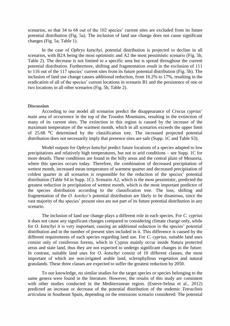
Abstract

Environmental change in terms of land use and climatic changes are posing a serious threat to

species distributions and extinctions. Thus in order to predict and mitigate against the effects

of environmental change both drivers should be accounted for. Two endemic plant species in

the Mediterranean island of Cyprus, Crocus cyprius and Ophrys kotschyi, were used as a case

study. We have coupled climate change scenarios, and land use change models with species

distribution models. Future land use scenarios were modelled by initially calculating the rate

of current land use changes between two time snapshots (2000 and 2006) on the island, and

based on these transition probabilities markov-chain cellular automata were used to generate

future land use changes for 2050. Climate change scenarios A1B, A2, B1 and B2A were

derived from the IPCC reports. Species’ climatic preferences were derived from their current

distributions using classification trees while habitats preferences were derived from the Red

Data Book of the Flora of Cyprus. A bioclimatic model for Crocus cyprius was built using

mean temperature of wettest quarter, max temperature of warmest month and precipitation

seasonality, while for Ophrys kotchyi the bioclimatic model was built using precipitation of

wettest month, mean temperature of warmest quarter, isothermality, precipitation of coldest

quarter, and annual precipitation. Sequentially, simulation scenarios were performed

regarding future species distributions by accounting climate alone and both climate and land

use changes. The distribution of the two species resulting from the bioclimatic models was

then filtered by future land use changes, providing the species’ projected potential

distribution. The species’ projected potential distribution varies depending on the type and

scenario used, but many of both species’ current sites/locations are projected to be outside

their future potential distribution. Our results demonstrate the importance of including both

land use and climatic changes in predictive species modeling.

Keywords

Spatio-temporal computation; Species distribution modelling; land use changes; climatic

changes; habitat modification; model coupling; endemic species; Crocus cyprius; Ophrys

kotschyi

Introduction

Climate and land use changes are two of the main causes for biodiversity loss

worldwide, while their combined effects may be greater than either of these factors acting

alone (de Chazal and Rounsevell, 2009). Climate change has already affected species

distribution, abundance, phenology and interactions, while even greater impacts are expected

in the future (Rosenzweig et al., 2007) with three major options for threatened species: (a)

extinction, (b) evolution and subsequent adaptation and (c) shifting its geographic range to

more favourable conditions (Moustakas and Evans, 2013). However, the rate at which

climate change is happening today is often faster than the ability of some species to disperse

or adapt, while other factors such as land use change and habitat fragmentation impede their

ability to move to suitable areas (Thuiller et al., 2005).

Climate change models simulate the change in climate due to the accumulation of

greenhouse gases, based on the current understanding of atmospheric physics and chemistry

(Hannah, 2010). The Intergovernmental Panel on Climate Change (IPCC) has produced a

range of emission scenarios for use in global climate models that predict future climate

(IPCC, 2013). The latest IPCC report is based on alternative concentrations of greenhouse

gases without being associated with any socio-economic scenario, but instead could result

from different combinations of economic, technological, demographic, policy, and

institutional futures (IPCC, 2013). This change facilitates better integration of socio-

economic factors, such as land use changes into future projections.

Species Distribution Models (SDMs) use information on the locations of species and

their corresponding environmental covariates, creating statistical functions to be projected in

areas or time periods where environmental parameters are known but species distribution is

unknown, providing inference for potentially suitable sites (Brotons et al., 2004).

In addition to climate change, the destruction, fragmentation and degradation of

habitats due to changes in land use are among the strongest pressures on biodiversity (EEA,

2010). In analogy to climate modelling, land use change models use a variety of approaches

to assess and project the future role of land use change on biodiversity, soil degradation, the

ability of biological systems to support human needs and the vulnerability of places and

people to climatic, economic, or sociopolitical perturbations (Zhang et al., 2014). The

development of land use change scenarios allows their integration into SDMs alongside

dynamic climatic variables which can significantly improve a model’s explanatory and

predictive ability at fine scales (Martin et al., 2013). Land use can be incorporated into the

model as static variables that do not change over time (Iverson and Prasad, 2002), or as

dynamic variables that change under different scenarios (Schweiger et al., 2012).

Despite the fact the combined effects of climate and land use change affect species

distributions (Martin et al., 2013), only a small number of SDMs predict species distribution

based on both of these factors (e.g. Esteve-Selma, et al., 2012; Schweiger, et al., 2012;

Heubes, et al., 2013), while most SDMs that combine climatic variables with land use

variables, only use dynamic variables for climate, while land use is considered stable (Martin

et al., 2013). Dynamic model coupling (Verdin et al., 2014) of climate models and land use

models can be employed to account for the interaction between both effects in projected

future conditions (Evans et al., 2013a).

Cyprus is a biodiversity hotspot (Myers et al., 2000) which is expected to become

warmer and dryer (Hadjinicolaou et al., 2011). At the same time, the increased pressure for

urban and tourism development in Cyprus is leading to significant changes in land uses

(Eurostat, 2012). Thus, the island of Cyprus is an ideal study area because of the major

climate and land use changes expected in the near future, the presence of a multitude of

threatened endemic species and the absence of similar studies in the region to date. We

sought to quantify the combined effects of climatic and land use changes on two plant

endemic species.

Materials and Methods

Study area

Cyprus is the third largest Mediterranean island, with an area of 9251 Km2. The climate

is Mediterranean, with hot and dry summers from June to September (little or no rainfall,

average maximum temperatures up to 36°C), rainy but mild winters from November to

March and two short transitional seasons, autumn and spring. For detailed information

regarding the geomorphology and biogeography of the island see Supp. 1A.

Target species

The target species are Crocus cyprius Boiss. & Kotschy and Ophrys kotschyi H. Fleischm. &

Sofi, both endemic to Cyprus, and categorized as vulnerable under the IUCN classification

(Tsintides et al., 2007). The criteria considered to target these two species were: (i) high risk

of extinction (ii) endemism (iii) high number of data occurrences/location relative to other

available species (iv) significant differences between their distributions, as Crocus cyprius

only occurs in the Troodos Mountains, while Ophrys kotschyi occurs almost everywhere in

Cyprus except the Troodos Mountains. For additional information regarding the target

species see Table S1 in Supp. 1A.

Data

Species distribution data were obtained from the Red Data Book of the Flora of Cyprus

(Tsintides et al., 2007), in the form of true presence points. The data were collected during a

systematic extensive survey between 2002 and 2006 (Tsintides at al., 2007).

There were 102 true presences for C. cyprius and 117 for O. kotschyi.. From these, a set

of “theoretical” presences were derived for each species; these comprised centres of cells of

the potential habitat, i.e. the entire area with a suitable altitude, soil and land use, within

which at least one true presence had been recorded. Absence data were created artificially,

from background data of the entire potential habitat of each species; “these comprised the

centres of cells of the potential habitat where no true presence had been recorded. This was

done in order to provide a sample of the set of conditions available to the species in the

region and not to pretend that the species is absent in the selected sites (Phillips , et al., 2009).

The data were then weighted to simulate prevalence 0.5, i.e. the total weight of presence is

equal to the total weight of absences (Barbet-Massin et al., 2012).

Bioclimatic data were obtained from Worldclim database, Version 1.4 (release 3),

which is available on www.worldclim.org (Hijmans et al., 2005). The bioclimatic variables

used are shown in Table S2 in Supp. 1B. Future bioclimatic data were also obtained from

Worldclim for the year 2050, according to GCM HadCM3 (Hadley Centre Coupled Model,

Version 3) and A1B, A2, B1 and B2A SRES emission scenarios. Each scenario is based on a

different “storyline” and scenario family (A1, A2, B1 or B2), representing different

demographic, social, economic, technological, and environmental developments (IPCC,

2013). The four storylines combine two sets of divergent tendencies: one set varying between

strong economic values (A1 and A2 families) and strong environmental values (B1 and B2

families), the other set between increasing globalization (A1 and B1 families) and increasing

regionalization (A2 and B2 families) (Nakicenovic & Swart, 2000).

. Land use data for 2000 and 2006 were obtained from CORINE database, available on

http://www.eea.europa.eu/data-and-maps. The resolution for both the current and the future

bioclimatic data was 0.71 Km2 while for the land-use data 250 m x 250 m.

Habitat preferences were determined based on the information provided in The Red

Data Book of the Flora of Cyprus, which was the result of a systematic study of all available

information on the threatened plants of Cyprus, in combination with field work (Tsintides et

al., 2007). The combination of suitable altitude, soil and land use, as described in Tsintides et

al. (2007) was defined as the species current potential habitat when using current land use

and as future potential habitat when using future land use in ArcGIS (http://www.esri.com).

SDMs

The SDMs were created using Classification Trees (CT), a machine learning method

used to create predictive models (Figures 2 and 3). The method predicts the value of a

dependent variable with a finite set of values, from the values of a set of independent

variables (Ji et al., 2013). The main advantage of this method is that it does not require a

specific type of data or that they follow a specific statistical distribution. The evaluation of

the predictive accuracy of the model was measured using Cohen's Kappa (Congalton, 1991)

and the "area under the curve” (AUC) of Receiver Operating Characteristic plot (ROC plot)

(Fielding and Bell, 1997). The Classification Tree is considered to represent each species’

“bioclimatic envelope” or “bioclimatic space”, which is defined as the climatic component of

the fundamental ecological niche, or the ‘climatic niche’ (Pearson and Dawson, 2003). We

used SPSS version 20 for the statistical analysis (http://www-

01.ibm.com/software/analytics/spss/).

Land use prediction

Future land use was predicted with an integration of Markov chain and Cellular

Automata (Figure 4). Markov chain is a technique that has been widely used to predict

changes in vegetation and which predicts future changes based on the rate of previous

changes (Arsanjani et al., 2011). The main disadvantage of the Markov chain is its lack of

spatial dimension: it gives accurate information on the transition probabilities of each land

use type to another, but provides no information on the spatial distribution of changes

(Eastman, 2003).

This problem is solved by combining Markov chain with Cellular Automata (Arsanjani

et al., 2011). Cellular Automata are digital entities that have the ability to change their state

based on the previous condition of themselves and their neighbours, based on a specific rule

(Moustakas et al., 2006).

In order to model land use changes we used two different time snapshots 2000 and

2006 of the Cyprus CORINE land-use maps. For each land use type we calculated the

transition probabilities to all the other land use types as well as the probability of no land use

changes (retain current land use type). This was implemented in a spatially explicit manner

i.e. transition probabilities were calculated for each location, where locations were

represented by 1 km grid cells. Thus, the transition probability depends not only on the cell’s

previous state but also on the state and rate of change of the neighbouring cells.

Climate and land use change integration

We generated future land use scenarios for 2050 using CA_MARKOV in Idrisi Selva

software (http://www.clarklabs.org(Eastman, 2003) (Figure 4). We used ArcGIS version 8

(www.esri.com) to map the modelled outputs of the species’ future potential distributions

based on bioclimatic modelling (bioclimatic envelope and future climate data). We then

combined the projected distribution for 2050 based on bioclimatic space with the current and

future potential habitat, producing future potential distributions based on climate change only

and on climate and land use changes respectively (Figure 5). This was done by simply taking

the cells in which projected distribution based on bioclimatic space and potential habitat

overlap. The methodology that was used is summarized in Figure 1.

Results

SDMs

The potential distribution of Crocus cyprius can be predicted using only three

bioclimatic variables as deduced from the classification tree: Mean Temperature of Wettest

Quarter, Max Temperature of Warmest Month and, and Precipitation Seasonality; (Fig. 2).

Model accuracy was “good” to “substantial” as indicated by Cohen’s Kappa and AUC values

of 0.719 and 0.859 respectively (Landis and Koch, 1977; Swets, 1988). The potential

distribution of Ophrys kotchyi’s can be predicted using five bioclimatic variables as deduced

from the classification tree: Precipitation of Wettest Month, Mean Temperature of Warmest

Quarter, Isothermality, Precipitation of Coldest Quarter, and Annual Precipitation; (Fig. 3).

Model accuracy was also good (Kappa = 0.619, AUC = 0.809). SDM performance measures

only relate to current distributions.

Land use prediction

The map of future land use produced from CORINE 2000 and 2006 maps using

CA_MARKOV indicated that the biggest increase in 2050 compared to 2006 is predicted for

artificial surfaces (Fig. 4). Non-irrigated arable land presents the greatest reduction, followed

by sclerophyllous vegetation and natural grasslands (Fig. 4). The classes with the lowest

predicted change are broad-leaved forest and mixed forest (Fig. 4).

Climate and land use change integration

Potential distributions of Crocus cyprius in present conditions, considering climate

change only and considering climate and land use change suggest that in scenario B2A its

potential distribution increases, while in all other scenarios it decreases, with A1B being the

most pessimistic (Fig. 5a; Table 1). The decreased potential distribution is limited at higher

altitudes, while the suitable areas at lower altitudes disappear. Shifting is predicted in all

scenarios, so that 34 to 68 out of the 102 species’ current sites are excluded from its future

potential distribution (Fig. 5a). The inclusion of land use change does not cause significant

changes (Fig. 5a; Table 1).

In the case of Ophrys kotschyi, potential distribution is projected to decline in all

scenarios, with B2A being the most optimistic and A2 the most pessimistic scenario (Fig. 5b,

Table 2). The decrease is not limited to a specific area but is spread throughout the current

potential distribution. Furthermore, shifting and fragmentation result in the exclusion of 111

to 116 out of the 117 species’ current sites from its future potential distribution (Fig. 5b). The

inclusion of land use change causes additional reduction, from 16.2% to 17%, resulting in the

eradication of all of the species’ current locations in scenario B1 and the persistence of one or

two locations in all other scenarios (Fig. 5b, Table 2).

Discussion

According to our model all scenarios predict the disappearance of Crocus cyprius’

main area of occurrence in the top of the Troodos Mountains, resulting in the extinction of

many of its current sites. The extinction in this region is caused by the increase of the

maximum temperature of the warmest month, which in all scenarios exceeds the upper limit

of 25.68 ⁰C determined by the classification tree. The increased projected potential

distribution does not necessarily imply that presence sites are safe (Supp. 1C and Table S3).

Model outputs for Ophrys kotschyi predict future locations of a species adapted to low

precipitations and relatively high temperatures, but not to arid conditions – see Supp. 1C for

more details. These conditions are found in the hilly areas and the central plain of Mesaoria,

where this species occurs today. Therefore, the combination of decreased precipitation of

wettest month, increased mean temperature of warmest quarter and decreased precipitation of

coldest quarter in all scenarios is responsible for the reduction of the species’ potential

distribution (Table S4 in Supp. 1C). Scenario A2, which is the most pessimistic, predicted the

greatest reduction in precipitation of wettest month, which is the most important predictor of

the species distribution according to the classification tree. The loss, shifting and

fragmentation of the O. kotshyi’s potential distribution are likely to be disastrous, since the

vast majority of the species’ present sites are not part of its future potential distribution in any

scenario.

The inclusion of land use change plays a different role in each species. For C. cyprius

it does not cause any significant changes compared to considering climate change only, while

for O. kotschyi it is very important, causing an additional reduction in the species’ potential

distribution and in the number of present sites included in it. This difference is caused by the

different requirements of each species regarding land use. For C. cyprius, suitable land uses

consist only of coniferous forests, which in Cyprus mainly occur inside Natura protected

areas and state land, thus they are not expected to undergo significant changes in the future.

In contrast, suitable land uses for O. kotschyi consist of 10 different classes, the most

important of which are non-irrigated arable land, sclerophyllous vegetation and natural

grasslands. These three classes are expected to suffer the greatest reduction by 2050.

To our knowledge, no similar studies for the target species or species belonging to the

same genera were found in the literature. However, the results of this study are consistent

with other studies conducted in the Mediterranean region. (Esteve-Selma et al., 2012)

predicted an increase or decrease of the potential distribution of the endemic Tetraclinis

articulata in Southeast Spain, depending on the emissions scenario considered: The potential

distribution increases in scenario B2 and severely reduced in scenario A2. This is in

agreement with our results for C. cyprius, but not with those of O. kotschyi, whose potential

distribution is predicted to decrease in all scenarios. Our results are also consistent with those

of (Vennetier and Ripert, 2009), who predict the disappearance of most forest areas with high

species richness in Southeast France by 2050, using bioclimatic modelling. The projected

limitation of C. cyprius’ potential distribution at higher altitudes agrees with the predictions

of other studies (Bell et al., 2014; Ferrarini et al.). In general the coupling of climate change

and land use change resulted in more restricted distributions for O. kotschyi is in agreement

with the predictions of other studies (de Chazal and Rounsevell, 2009).

Limitations, uncertainty and future directions

There are a number of limitations related with the methodology employed in the current

study. These include spatial and temporal resolution mismatch between the bioclimatic and

the species distribution data, the possibility of sampling bias on the species distribution data,

the quality and accuracy of the Worldclim (Hijmans et al., 2005) and CORINE data

(http://www.eea.europa.eu/data-and-maps). In addition SDMs are based on a number of

unrealistic assumptions (Evans et al., 2013a). These include considering that the model

quantifies the realized ecological niche (Pellissier et al., 2013) and that the species are in

equilibrium with the environment, ignoring biotic interactions (Matias et al., 2014) and

evolutionary and phenotypic changes as an adaptation to climate and land use change

(Moustakas and Evans, 2013), assuming full dispersion for both species (Rodríguez-Rey et

al., 2013) and training the model only in the realized environment (Maher et al., 2014). Also,

it is considered that the potential distribution is the geographic area that meets one or more

components of the fundamental ecological niche, when in fact the real potential distribution

includes the entire fundamental ecological niche. As a result, the actual future potential

distributions are likely to be under- or over- predicted (Jiménez-Valverde et al., 2008).

Although widely employed as a measure for SDM performance, AUC has been also criticised

(see Lobo et al. 2008). Other important sources of uncertainty were the creation of theoretical

presences and absences (Barbet-Massin et al., 2012). In addition predictions are often scale

specific while the interaction of species with their environment takes place at a variety of

scales (Bellamy et al., 2013).

Finally the inclusion of both climatic and land use variables introduces a new source of

uncertainty, through the different parameters and assumptions it brings (Conlisk et al., 2013).

However simple models do not lead to generality in their predictions and thus increasing

complexity may yield more realistic predictions (Evans et al., 2014; Evans et al., 2013b).

Here model coupling (Verdin et al., 2014) of bioclimatic modelling with the use of

markov chain cellular automata (Arsanjani et al., 2011) was employed. Alternatives may

include using individual based models (Gonzalès et al., 2013; Zhang et al., 2014) to model

both land use & climatic changes with a presence only or presence absence model output and

compare model outputs (Tonini et al., 2014) in an identical grid size. Although there is an

interaction effect between land use and climate changes, disentangling these is conceptually

complicated (see Lehsten et al. 2015) and is unaccounted for in this study.

The procedure developed herein can be used for any species where data is available and

provides a valuable and transferable method for understanding potential shifts in species

distributions. In addition the maps produced can guide actions on adaptation and mitigation

measures to climate change for the species studied, providing a useful tool for policy and

decision makers.

References

Arsanjani, J.J., Kainz, W., Mousivand, A.J., 2011. Tracking dynamic land-use change using

spatially explicit Markov Chain based on cellular automata: the case of Tehran.

International Journal of Image and Data Fusion 2, 329-345.

Barbet-Massin, M., Jiguet, F., Albert, C.H., Thuiller, W., 2012. Selecting pseudo-absences

for species distribution models: how, where and how many? Methods Ecol. Evol. 3,

327-338.

Bell, D.M., Bradford, J.B., Lauenroth, W.K., 2014. Mountain landscapes offer few

opportunities for high-elevation tree species migration. Glob. Change. Biol. 20, 1441-

1451.

Bellamy, C., Scott, C., Altringham, J., 2013. Multiscale, presence‐only habitat suitability

models: fine‐resolution maps for eight bat species. Journal of Applied Ecology 50, 892-

901.

Brotons, L., Thuiller, W., Araújo, M.B., Hirzel, A.H., 2004. Presence‐absence versus

presence‐only modelling methods for predicting bird habitat suitability. Ecography 27,

437-448.

Congalton, R.G., 1991. A review of assessing the accuracy of classifications of remotely

sensed data. Remote sensing of environment 37, 35-46.

Conlisk, E., Syphard, A.D., Franklin, J., Flint, L., Flint, A., Regan, H., 2013. Uncertainty in

assessing the impacts of global change with coupled dynamic species distribution and

population models. Glob. Change. Biol. 19, 858-869.

de Chazal, J., Rounsevell, M.D.A., 2009. Land-use and climate change within assessments of

biodiversity change: A review. Global Environmental Change 19, 306-315.

Eastman, J.R., 2003. IDRISI Kilimanjaro Tutorial., http://gisgeek.pdx.edu/G424-

GIS/KilimanjaroTutorial.pdf.

EEA, 2010. The European environment – state and outlook 2010: Synthesis.

Esteve-Selma, M., Martínez-Fernández, J., Hernández-García, I., Montávez, J., López-

Hernández, J., Calvo, J., 2012. Potential effects of climatic change on the distribution

of Tetraclinis articulata, an endemic tree from arid Mediterranean ecosystems. Climatic

Change 113, 663-678.

Eurostat, 2012. Agri-environmental indicator - land use change,

http://epp.eurostat.ec.europa.eu/statistics_explained/index.php/Agri-

environmental_indicator_-_land_use_change#Further_information.

Evans, M.R., Benton, T.G., Grimm, V., Lessells, C.M., O’Malley, M.A., Moustakas, A.,

Weisberg, M., 2014. Data availability and model complexity, generality, and utility: a

reply to Lonergan. Trends in Ecology & Evolution 29, 302-303.

Evans, M.R., Bithell, M., Cornell, S.J., Dall, S.R.X., Díaz, S., Emmott, S., Ernande, B.,

Grimm, V., Hodgson, D.J., Lewis, S.L., Mace, G.M., Morecroft, M., Moustakas, A.,

Murphy, E., Newbold, T., Norris, K.J., Petchey, O., Smith, M., Travis, J.M.J., Benton,

T.G., 2013a. Predictive systems ecology. Proceedings of the Royal Society B:

Biological Sciences 280.

Evans, M.R., Grimm, V., Johst, K., Knuuttila, T., de Langhe, R., Lessells, C.M., Merz, M., O

Malley, M.A., Orzack, S.H., Weisberg, M., Wilkinson, D.J., Wolkenhauer, O., Benton,

T.G., 2013b. Do simple models lead to generality in ecology? Trends in ecology &

evolution 28, 578-583.

Ferrarini, A., Rossi, G., Mondoni, A., Orsenigo, S., Prediction of climate warming impacts on

plant species could be more complex than expected. Evidence from a case study in the

Himalaya. Ecological Complexity.

Fielding, A.H., Bell, J.F., 1997. A review of methods for the assessment of prediction errors

in conservation presence/absence models. Environmental conservation 24, 38-49.

Gonzalès, R., Cardille, J.A., Parrott, L., 2013. Agent-based land-use models and farming

games on the social web—Fertile ground for a collaborative future? Ecological

Informatics 15, 14-21.

Hadjinicolaou, P., Giannakopoulos, C., Zerefos, C., Lange, M.A., Pashiardis, S., Lelieveld, J.,

2011. Mid-21st century climate and weather extremes in Cyprus as projected by six

regional climate models. Regional Environmental Change 11, 441-457.

Hannah, L., 2010. Climate change biology. Academic Press.

Hijmans, R.J., Cameron, S.E., Parra, J.L., Jones, P.G., Jarvis, A., 2005. Very high resolution

interpolated climate surfaces for global land areas. International journal of climatology

25, 1965-1978.

IPCC, 2013. Scenario Process For AR5., http://sedac.ipcc-

data.org/ddc/ar5_scenario_process/index.htm.

Iverson, L.R., Prasad, A.M., 2002. Potential redistribution of tree species habitat under five

climate change scenarios in the eastern US. Forest Ecology and Management 155, 205-

222.

Ji, Z., Li, N., Xie, W., Wu, J., Zhou, Y., 2013. Comprehensive assessment of flood risk using

the classification and regression tree method. Stoch Environ Res Risk Assess 27, 1815-

1828.

Jiménez-Valverde, A., Lobo, J.M., Hortal, J., 2008. Not as good as they seem: the importance

of concepts in species distribution modelling. Diversity and Distributions 14, 885-890.

Landis, J.R., Koch, G.G., 1977. The measurement of observer agreement for categorical data.

biometrics, 159-174.

Maher, S.P., Randin, C.F., Guisan, A., Drake, J.M., 2014. Pattern-recognition ecological

niche models fit to presence-only and presence–absence data. Methods Ecol. Evol. 5,

761-770.

Martin, Y., Van Dyck, H., Dendoncker, N., Titeux, N., 2013. Testing instead of assuming the

importance of land use change scenarios to model species distributions under climate

change. Global Ecol. & Biogeog. 22, 1204-1216.

Matias, M.G., Gravel, D., Guilhaumon, F., Desjardins-Proulx, P., Loreau, M., Münkemüller,

T., Mouquet, N., 2014. Estimates of species extinctions from species–area relationships

strongly depend on ecological context. Ecography 37, 431-442.

Moustakas, A., Evans, M.R., 2013. Integrating Evolution into Ecological Modelling:

Accommodating Phenotypic Changes in Agent Based Models. PloS One 8, e71125.

Moustakas, A., Silvert, W., Dimitromanolakis, A., 2006. A spatially explicit learning model

of migratory fish and fishers for evaluating closed areas. Ecol. Model. 192, 245-258.

Myers, N., Mittermeier, R.A., Mittermeier, C.G., Da Fonseca, G.A., Kent, J., 2000.

Biodiversity hotspots for conservation priorities. Nature 403, 853-858.

Pearson, R.G., Dawson, T.P., 2003. Predicting the impacts of climate change on the

distribution of species: are bioclimate envelope models useful? Global Ecol. &

Biogeog. 12, 361-371.

Pellissier, L., Bråthen, K.A., Vittoz, P., Yoccoz, N.G., Dubuis, A., Meier, E.S., Zimmermann,

N.E., Randin, C.F., Thuiller, W., Garraud, L., 2013. Thermal niches are more

conserved at cold than warm limits in arctic‐alpine plant species. Global Ecol. &

Biogeog. 22, 933-941.

Rodríguez-Rey, M., Jiménez-Valverde, A., Acevedo, P., 2013. Species distribution models

predict range expansion better than chance but not better than a simple dispersal model.

Ecol. Model. 256, 1-5.

Rosenzweig, C., Casassa, G., Karoly, D.J., Imeson, A., Liu, C., Menzel, A., Rawlins, S.,

Root, T.L., Seguin, B., Tryjanowski, P., 2007. Assessment of observed changes and

responses in natural and managed systems, In: Parry, M.L., Canziani, O.F., Palutikof,

J.P., Linden, P.J.v.d., Hanson, C.E. (Parry, M.L., Canziani, O.F., Palutikof, J.P.,

Linden, P.J.v.d., Hanson, C.E.(Parry, M.L., Canziani, O.F., Palutikof, J.P., Linden,

P.J.v.d., Hanson, C.E.s), Climate Change 2007: Impacts, Adaptation and Vulnerability

Contribution of Working Group II to the Fourth Assessment Report of the

Intergovernmental Panel on Climate Change. Cambridge University Press, Cambridge,

UK, pp. 79-131.

Schweiger, O., Heikkinen, R.K., Harpke, A., Hickler, T., Klotz, S., Kudrna, O., Kühn, I.,

Pöyry, J., Settele, J., 2012. Increasing range mismatching of interacting species under

global change is related to their ecological characteristics. Global Ecol. & Biogeog. 21,

88-99.

Swets, J.A., 1988. Measuring the accuracy of diagnostic systems. Science 240, 1285-1293.

Thuiller, W., Lavorel, S., Araújo, M.B., Sykes, M.T., Prentice, I.C., 2005. Climate change

threats to plant diversity in Europe. Proceedings of the National Academy of Sciences

of the United States of America 102, 8245-8250.

Tonini, F., Hochmair, H.H., Scheffrahn, R.H., DeAngelis, D.L., 2014. Stochastic spread

models: A comparison between an individual-based and a lattice-based model for

assessing the expansion of invasive termites over a landscape. Ecological Informatics

24, 222-230.

Tsintides, T., Christodoulou, C., Delipetrou, P., Georghiou, K., 2007. The red data book of

the flora of Cyprus. Cyprus Forestry Association, Lefkosia, 465.

Vennetier, M., Ripert, C., 2009. Forest flora turnover with climate change in the

Mediterranean region: a case study in Southeastern France. Forest ecology and

management 258, S56-S63.

Verdin, A., Rajagopalan, B., Kleiber, W., Katz, R., 2014. Coupled stochastic weather

generation using spatial and generalized linear models. Stoch Environ Res Risk Assess,

1-10.

Zhang, H., Jin, X., Wang, L., Zhou, Y., Shu, B., 2014. Multi-agent based modeling of

spatiotemporal dynamical urban growth in developing countries: simulating future

scenarios of Lianyungang city, China. Stoch Environ Res Risk Assess, 1-16.

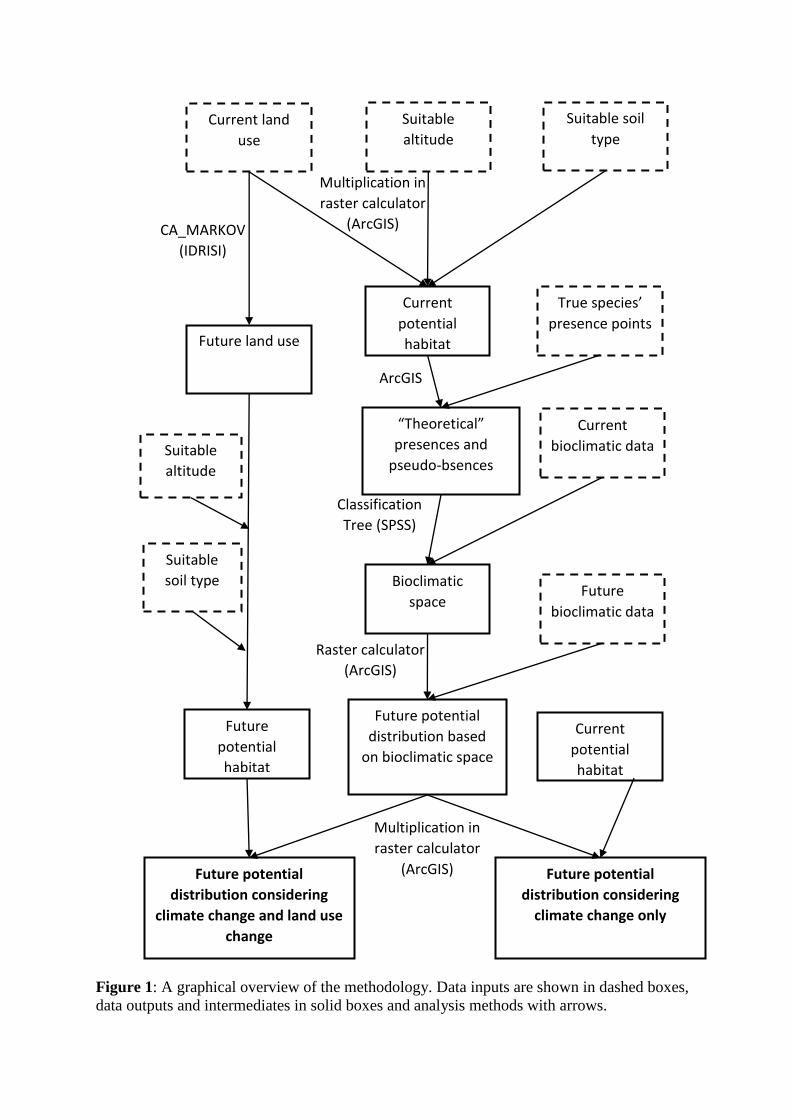
Figure 1: A graphical overview of the methodology. Data inputs are shown in dashed boxes,

data outputs and intermediates in solid boxes and analysis methods with arrows.

Future potential

distribution based

on bioclimatic space

Current land

use

Suitable

altitude

Suitable soil

type

Current

potential

habitat

“Theoretical”

presences and

pseudo-bsences

Bioclimatic

space

CA_MARKOV

(IDRISI)

Future land use

Future

potential

habitat

True species’

presence points

Current

bioclimatic data

Future

bioclimatic data

Current

potential

habitat

Future potential

distribution considering

climate change and land use

change

Future potential

distribution considering

climate change only

Multiplication in

raster calculator

(ArcGIS)

ArcGIS

Raster calculator

(ArcGIS)

Classification

Tree (SPSS)

Multiplication in

raster calculator

(ArcGIS)

Suitable

altitude

Suitable

soil type

Figure.2. Classification tree for Crocus cyprius. As shown, three bioclimatic variables

determine the distribution of C. cyprius: bio8 (Mean Temperature of Wettest Quarter), bio5

(Max Temperature of Warmest Month) and bio15 (Precipitation Seasonality). If bio8 is less

than or equal to 3.92 °C, the species can only be present if bio5 is less or equal to 25.68 °C. If

bio8 is more than 3.92 °C, the species can be present either when bio15 is less than or equal

to 92%.

Figure 3. Classification tree for Ophrys kotschyi. A shown, five bioclimatic variables

determine the distribution of O. kotschyi: bio13 (Precipitation of Wettest Month), bio10

(Mean Temperature of Warmest Quarter), bio3 (Isothermality), bio19 (Precipitation of

Coldest Quarter) and bio12 (Annual Precipitation). If bio13 is less than or equal to 110.5 mm,

the species can be present either when bio10 is less than or equal to 26.65 °C and bio3 is less

than or equal to 42.5, or when bio10 is more than 26.65 °C and bio19 is between 172.5 mm

and 183.5 mm. If bio13 is more than 110.5 mm, the species can only be present if bio13 is

more than 142.5 mm and bio12 is less than or equal to 622.5 mm.

Figure 4. Prediction of land use in 2050, using CORINE land-cover data for 2000 and 2006

and CA-MARKOV. All land use classes and their codes are listed in Table S5 in Supp. 1.

CA_MARKOV

Figure 5. Potential distribution for Crocus cyprius (a) and Ophrys kotschyi (b) in current

conditions (top), in 2050 considering only climate change (middle) and in 2050 considering

climate and land use change (bottom). All land use classes and their codes are listed in Table

S5 in Supp. 1.

Current

distribution

2050 –

Climate

change

only

(a) Crocus cyprius (b) Ophrys kotschyi

2050 –

Climate and

land use

change

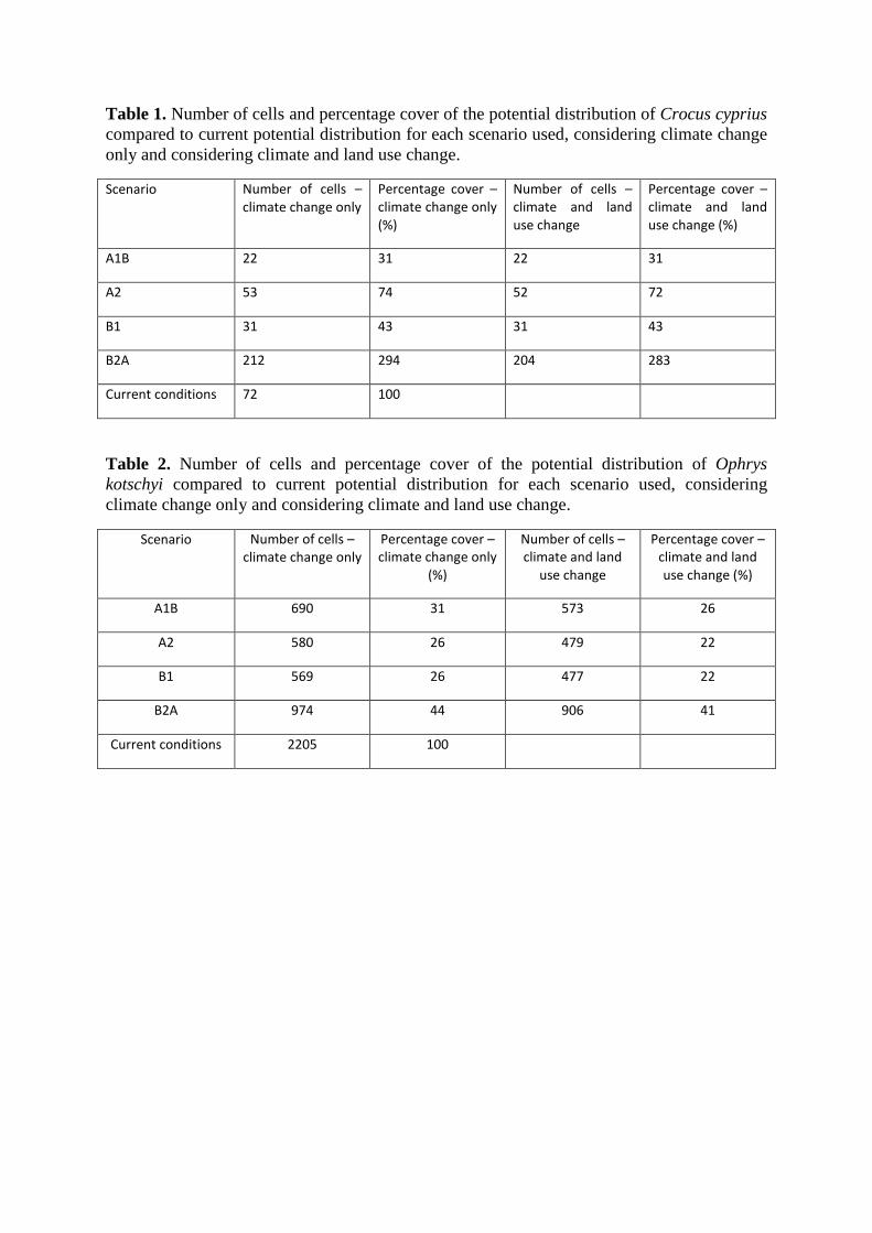
Table 1. Number of cells and percentage cover of the potential distribution of Crocus cyprius

compared to current potential distribution for each scenario used, considering climate change

only and considering climate and land use change.

Scenario Number of cells – climate change only

Percentage cover – climate change only (%)

Number of cells – climate and land use change

Percentage cover – climate and land use change (%)

Α1Β 22 31 22 31

Α2 53 74 52 72

Β1 31 43 31 43

Β2Α 212 294 204 283

Current conditions 72 100

Table 2. Number of cells and percentage cover of the potential distribution of Ophrys

kotschyi compared to current potential distribution for each scenario used, considering

climate change only and considering climate and land use change.

Scenario Number of cells – climate change only

Percentage cover – climate change only

(%)

Number of cells – climate and land

use change

Percentage cover – climate and land use change (%)

Α1Β 690 31 573 26

Α2 580 26 479 22

Β1 569 26 477 22

Β2Α 974 44 906 41

Current conditions 2205 100

Supplement 1

Supplement 1A

The main geomorphologic zones of Cyprus are the Troodos Mountains in the southwest, the

Pentadaktylos mountain range to the north, the central valley of Messaoria and the coastal

zone. The main types of land cover include high forests on the Troodos and Pentadaktylos

ranges, while the lower hills are dominated by shrubs alternating with built-up areas and

cultivations. The plain of Messaoria and the coastal zone are mainly covered by cultivations

and habitations, although some parts of natural or semi-natural vegetation still persist

(Tsintides et al., 2007). Cyprus is predicted to be severely affected by climate change

(Lelieveld et al., 2013). (Hadjinicolaou et al., 2011), predict the transition of the island to a

warmer state for the period from 2026 to 2050, with increase in both the maximum and the

minimum temperature by 1 °C to 2 °C and decline in rainfall by 8.2%.

Table S1: Target species information (IUCN, 2013; Tsintides et al., 2007). Both are included

in Annex II of the Habitats Directive (92/43/EEC), and in Appendix I of the Bern Convention

Species Crocus cyprius Ophrys kotschyi

Description perennial herb perennial orchid

Population over 11,500 plants in the

Troodos Mountains

at least 30 locations around the

island usually forming small

colonies of 10 to 100 plants

Soil type igneous formations limestone formations

Altitude 1050 – 1950 m 0 – 900 m

Land use type pine forest openings,

Juniperus foetidissima forests

and edges of peat grasslands

phrygana and maquis, grassy

slopes, field margins, sparse

pine forests and moist places

Threats trampling and construction,

natural fires, climate change

and military construction

land development, tourism

infrastructure, overcollection

and failure in sexual

reproduction

Protection all subpopulations within the

Natura 2000 network

All subpopulations in state

forests or in Natura 2000 areas

---------------------------------------------------------------------------------------------------------------

---------------------

Supplement 1B

Table S2. Bioclimatic variables used in the model

BIO1 Annual Mean Temperature

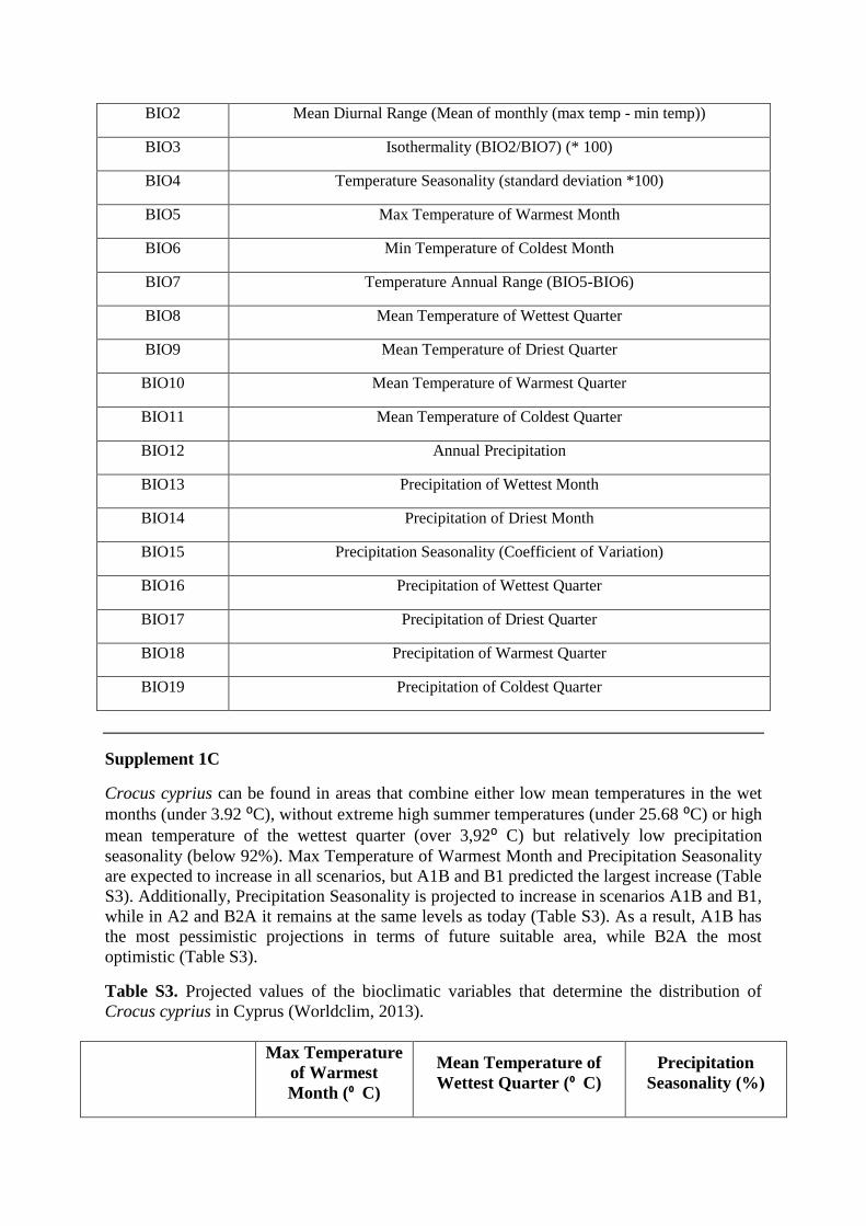
BIO2 Mean Diurnal Range (Mean of monthly (max temp - min temp))

BIO3 Isothermality (BIO2/BIO7) (* 100)

BIO4 Temperature Seasonality (standard deviation *100)

BIO5 Max Temperature of Warmest Month

BIO6 Min Temperature of Coldest Month

BIO7 Temperature Annual Range (BIO5-BIO6)

BIO8 Mean Temperature of Wettest Quarter

BIO9 Mean Temperature of Driest Quarter

BIO10 Mean Temperature of Warmest Quarter

BIO11 Mean Temperature of Coldest Quarter

BIO12 Annual Precipitation

BIO13 Precipitation of Wettest Month

BIO14 Precipitation of Driest Month

BIO15 Precipitation Seasonality (Coefficient of Variation)

BIO16 Precipitation of Wettest Quarter

BIO17 Precipitation of Driest Quarter

BIO18 Precipitation of Warmest Quarter

BIO19 Precipitation of Coldest Quarter

Supplement 1C

Crocus cyprius can be found in areas that combine either low mean temperatures in the wet

months (under 3.92 ⁰C), without extreme high summer temperatures (under 25.68 ⁰C) or high

mean temperature of the wettest quarter (over 3,92⁰ C) but relatively low precipitation

seasonality (below 92%). Max Temperature of Warmest Month and Precipitation Seasonality

are expected to increase in all scenarios, but A1B and B1 predicted the largest increase (Table

S3). Additionally, Precipitation Seasonality is projected to increase in scenarios A1B and B1,

while in A2 and B2A it remains at the same levels as today (Table S3). As a result, A1B has

the most pessimistic projections in terms of future suitable area, while B2A the most

optimistic (Table S3).

Table S3. Projected values of the bioclimatic variables that determine the distribution of

Crocus cyprius in Cyprus (Worldclim, 2013).

Max Temperature

of Warmest

Month (⁰ C)

Mean Temperature of

Wettest Quarter (⁰ C)

Precipitation

Seasonality (%)

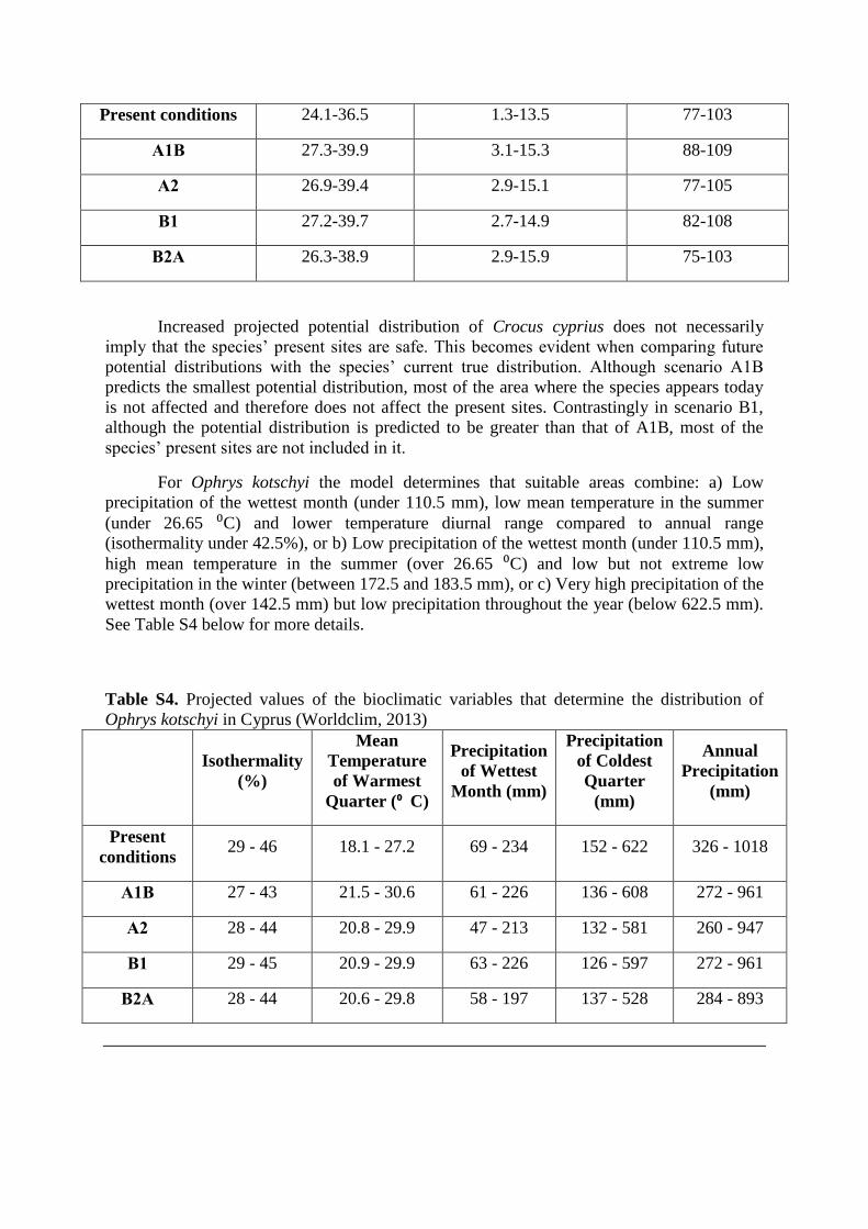
Present conditions 24.1-36.5 1.3-13.5 77-103

Α1Β 27.3-39.9 3.1-15.3 88-109

Α2 26.9-39.4 2.9-15.1 77-105

Β1 27.2-39.7 2.7-14.9 82-108

Β2Α 26.3-38.9 2.9-15.9 75-103

Increased projected potential distribution of Crocus cyprius does not necessarily

imply that the species’ present sites are safe. This becomes evident when comparing future

potential distributions with the species’ current true distribution. Although scenario A1B

predicts the smallest potential distribution, most of the area where the species appears today

is not affected and therefore does not affect the present sites. Contrastingly in scenario B1,

although the potential distribution is predicted to be greater than that of A1B, most of the

species’ present sites are not included in it.

For Ophrys kotschyi the model determines that suitable areas combine: a) Low

precipitation of the wettest month (under 110.5 mm), low mean temperature in the summer

(under 26.65 ⁰C) and lower temperature diurnal range compared to annual range

(isothermality under 42.5%), or b) Low precipitation of the wettest month (under 110.5 mm),

high mean temperature in the summer (over 26.65 ⁰C) and low but not extreme low

precipitation in the winter (between 172.5 and 183.5 mm), or c) Very high precipitation of the

wettest month (over 142.5 mm) but low precipitation throughout the year (below 622.5 mm).

See Table S4 below for more details.

Table S4. Projected values of the bioclimatic variables that determine the distribution of

Ophrys kotschyi in Cyprus (Worldclim, 2013)

Isothermality

(%)

Mean

Temperature

of Warmest

Quarter (⁰ C)

Precipitation

of Wettest

Month (mm)

Precipitation

of Coldest

Quarter

(mm)

Annual

Precipitation

(mm)

Present

conditions 29 - 46 18.1 - 27.2 69 - 234 152 - 622 326 - 1018

Α1Β 27 - 43 21.5 - 30.6 61 - 226 136 - 608 272 - 961

Α2 28 - 44 20.8 - 29.9 47 - 213 132 - 581 260 - 947

Β1 29 - 45 20.9 - 29.9 63 - 226 126 - 597 272 - 961

Β2Α 28 - 44 20.6 - 29.8 58 - 197 137 - 528 284 - 893

Table S5. Land use classes and their corresponding codes.

Reclassification

code

CLC

CODE LABEL 1 LABEL 2 LABEL 3

1

Artificial

surfaces - -

2 211

Agricultural

areas

Arable land Non-irrigated arable land

3 212 Arable land Permanently irrigated land

4 221 Permanent crops Vineyards

5 222 Permanent crops Fruit trees and berry plantations

6 223 Permanent crops Olive groves

7 231 Pastures Pastures

8 241 Heterogeneous

agricultural areas

Annual crops associated with

permanent crops

9 242 Heterogeneous

agricultural areas Complex cultivation patterns

10 243 Heterogeneous

agricultural areas

Land principally occupied by

agriculture, with significant areas of

natural vegetation

11 311

Forest and

semi

natural

areas

Forests Broad-leaved forest

12 312 Forests Coniferous forest

13 313 Forests Mixed forest

14 321

Scrub and/or

herbaceous vegetation

associations

Natural grasslands

15 323

Scrub and/or

herbaceous vegetation

associations

Sclerophyllous vegetation

16 324

Scrub and/or

herbaceous vegetation

associations

Transitional woodland-shrub

17 331 Open spaces with

little or no vegetation Beaches, dunes, sands

18 332 Open spaces with

little or no vegetation Bare rocks

19 333 Open spaces with

little or no vegetation Sparsely vegetated areas

20 334 Open spaces with

little or no vegetation Burnt areas

21 411 Wetlands

Inland wetlands Inland marshes

22 421 Maritime wetlands Salt marshes

23

Water

bodies - -

References:

Hadjinicolaou, P., Giannakopoulos, C., Zerefos, C., Lange, M.A., Pashiardis, S., Lelieveld, J.,

2011. Mid-21st century climate and weather extremes in Cyprus as projected by six

regional climate models. Regional Environmental Change 11, 441-457.

IUCN, 2013. Crocus cyprius, http://www.iucnredlist.org/details/162216/0.

Lelieveld, J., Hadjinicolaou, P., Kostopoulou, E., Giannakopoulos, C., Pozzer, A., Tanarhte,

M., Tyrlis, E., 2013. Model projected heat extremes and air pollution in the eastern

Mediterranean and Middle East in the twenty-first century. Regional Environmental

Change, 1-13.

Tsintides, T., Christodoulou, C., Delipetrou, P., Georghiou, K., 2007. The red data book of

the flora of Cyprus. Cyprus Forestry Association, Lefkosia, 465.

Worldclim, 2013. Global Climate Data. Free climate data for ecological modeling and GIS,

http://www.worldclim.org.