Embed Size (px)
Citation preview
MODELLING RADIO IMAGING METHOD DATA USING ELECTRIC DIPOLES IN A
HOMOGENOUS WHOLE SPACE
by
Tomas Naprstek
A thesis submitted in partial fulfillment
of the requirements for the degree of
Master of Science (MSc) in Geology
The Faculty of Graduate Studies
Laurentian University
Sudbury, Ontario, Canada
© Tomas Naprstek, 2014
ii
iii
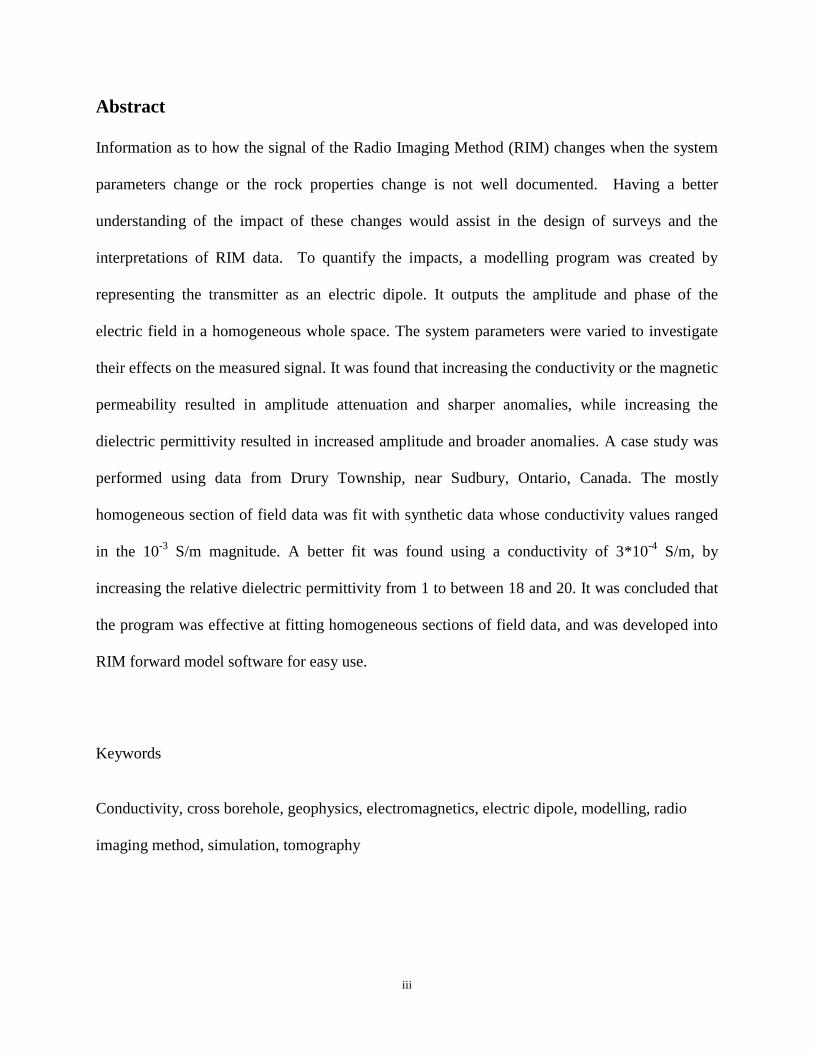
Abstract
Information as to how the signal of the Radio Imaging Method (RIM) changes when the system
parameters change or the rock properties change is not well documented. Having a better
understanding of the impact of these changes would assist in the design of surveys and the
interpretations of RIM data. To quantify the impacts, a modelling program was created by
representing the transmitter as an electric dipole. It outputs the amplitude and phase of the
electric field in a homogeneous whole space. The system parameters were varied to investigate
their effects on the measured signal. It was found that increasing the conductivity or the magnetic
permeability resulted in amplitude attenuation and sharper anomalies, while increasing the
dielectric permittivity resulted in increased amplitude and broader anomalies. A case study was
performed using data from Drury Township, near Sudbury, Ontario, Canada. The mostly
homogeneous section of field data was fit with synthetic data whose conductivity values ranged
in the 10-3
S/m magnitude. A better fit was found using a conductivity of 3*10-4
S/m, by
increasing the relative dielectric permittivity from 1 to between 18 and 20. It was concluded that
the program was effective at fitting homogeneous sections of field data, and was developed into
RIM forward model software for easy use.
Keywords
Conductivity, cross borehole, geophysics, electromagnetics, electric dipole, modelling, radio
imaging method, simulation, tomography

iv
Acknowledgments
I would like thank my supervisor, Dr. Richard Smith for his support and knowledge through the
research process. His guidance and assistance was invaluable. I would also like to thank my
office colleagues Christoph Schaub, Omid Mahmoodi, and Yongxing Li for their general
assistance and geophysics knowledge, and specifically Christoph for his proofreading skills
throughout my degree. I would like to acknowledge KGHM International, Sudbury Integrated
Nickel Operations A Glencore Company, Vale, Wallbridge Mining Company, the Centre for
Excellence in Mining Innovation (CEMI), the Mineral Exploration Research Centre (MERC),
and NSERC for support and funding. I would also like to thank Sudbury Integrated Nickel
Operations for releasing the field data I used in my case study. Finally I would like to thank my
good friend Benjamin Nicholls for his assistance in brainstorming several times throughout my
research.
v
Table of Contents
Abstract .......................................................................................................................................... iii
Acknowledgments.......................................................................................................................... iv
Table of Contents ............................................................................................................................ v
List of Tables ................................................................................................................................. vi
List of Figures ............................................................................................................................... vii
1 Introduction .................................................................................................................................. 1
2 Method ......................................................................................................................................... 4
3 Analysis...................................................................................................................................... 10
3.1 Finite Dipole ........................................................................................................................ 10
3.2 Parameter Investigation ....................................................................................................... 15
3.2.1 Electrical properties ...................................................................................................... 15
3.2.2 Frequency variation ...................................................................................................... 29
3.2.3 Angles ........................................................................................................................... 35
3.3 Discussion ........................................................................................................................... 37
4 Survey from Drury, Sudbury ..................................................................................................... 38
5 Forward Modelling Program ...................................................................................................... 54
6 Conclusions ................................................................................................................................ 56
7 References .................................................................................................................................. 60
Appendix A: Noise Level ............................................................................................................. 63
Appendix B: Case Study Synthetic Data Cusps ........................................................................... 67
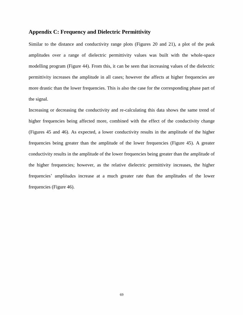
Appendix C: Frequency and Dielectric Permittivity .................................................................... 69

vi
List of Tables
Table 1. Standard parameter values used in calculations. ............................................................ 15
Table 2. Summary of the “Rules of Thumbs”............................................................................... 28
Table 3. Summary of the "Rules of Thumbs" in terms of α and β. ............................................... 29
vii
List of Figures
Figure 1. The basic setup of a RIM survey. The transmitter is located in one borehole, with the
receiver in another borehole. The transmitter is set at a number of locations in one hole, and a
series of measurements are taken with the receiver at multiple locations in another hole. The
amplitude plot is built from the receiver data, and shows conductive zones/bodies where the
attenuation of the signal is greater. ................................................................................................. 2
Figure 2: The RIM geometric configuration, listing all variables involved in the calculations. .... 5
Figure 3. The geometric variables pertaining to the transmitter reference frame x and z distance
values. ............................................................................................................................................. 7
Figure 4. Sample of the modelling code the output showing amplitude and phase of the electric
field that would be measured at receiver positions ranging from 250 m above (-250 m) to 250 m
below (+250 m) the transmitter depth. This is for a parallel borehole system (θtrans = θreceive = 0),
borehole separation x = 500 m, conductivity = 10-4
S/m. ............................................................. 10
Figure 5. Two approximations for a 10 m finite dipole. In the top panel, the finite dipole is
(poorly) approximated by a single infinitesimal dipole at the center of the 10 m finite dipole. In
the bottom panel, the finite dipole is approximated by five 2m dipoles distributed evenly over the
10 m length. There are three receiver positions on the right hand side. ....................................... 11
Figure 6: A plot depicting the difference in magnitude between a transmitter calculated as a
single 10 m dipole, and a transmitter calculated as ten evenly spaced 1 m dipoles. Each curve is
for a different borehole separation and/or whole-space conductivity. The cusps in the dashed and
dotted cases represent a switch in the sign of the magnitude difference, as the amplitudes begin
as greater than the 10 m dipole case’s amplitude, before falling in magnitudes to less than that of
the 10 m dipole case’s amplitude. ................................................................................................. 13
viii
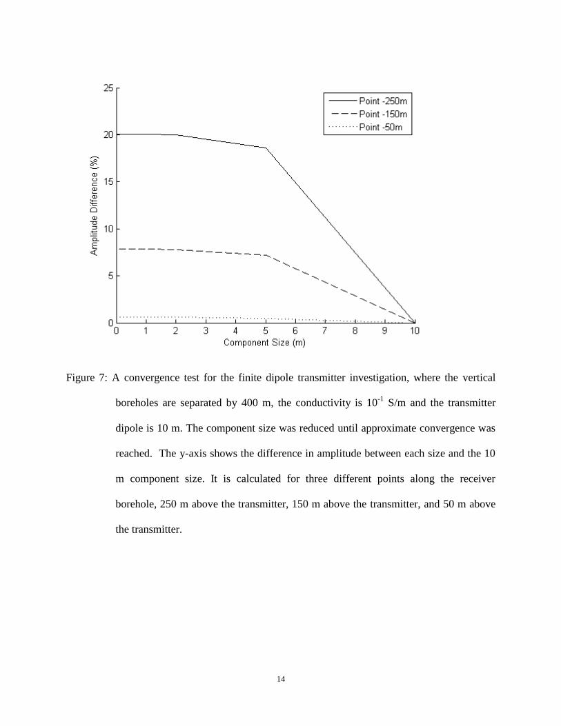
Figure 7: A convergence test for the finite dipole transmitter investigation, where the vertical
boreholes are separated by 400 m, the conductivity is 10-1
S/m and the transmitter dipole is 10 m.
The component size was reduced until approximate convergence was reached. The y-axis shows
the difference in amplitude between each size and the 10 m component size. It is calculated for
three different points along the receiver borehole, 250 m above the transmitter, 150 m above the
transmitter, and 50 m above the transmitter.................................................................................. 14
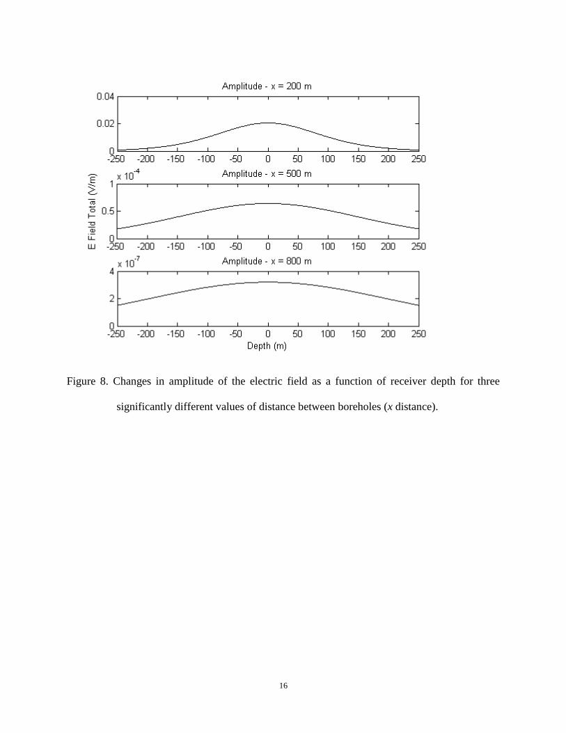
Figure 8. Changes in amplitude of the electric field as a function of receiver depth for three
significantly different values of distance between boreholes (x distance). ................................... 16
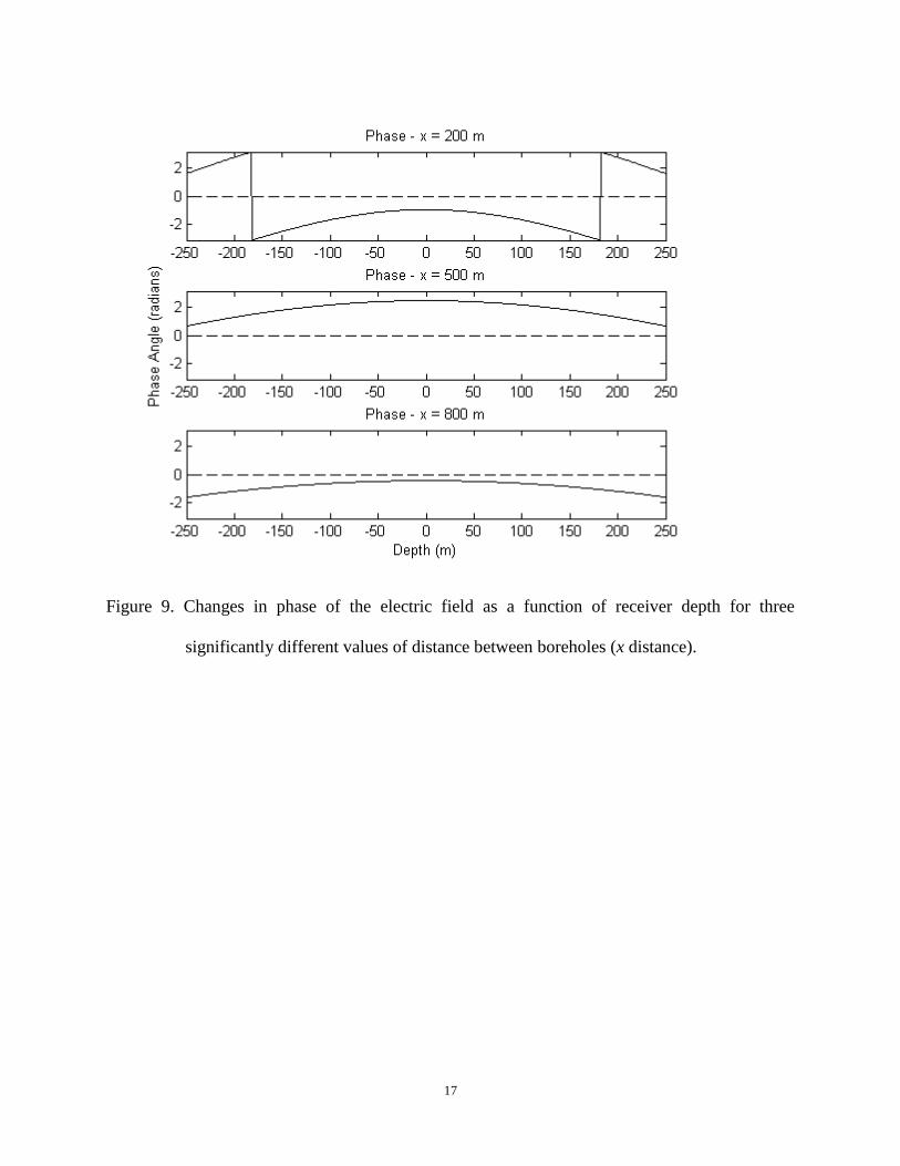
Figure 9. Changes in phase of the electric field as a function of receiver depth for three
significantly different values of distance between boreholes (x distance). ................................... 17
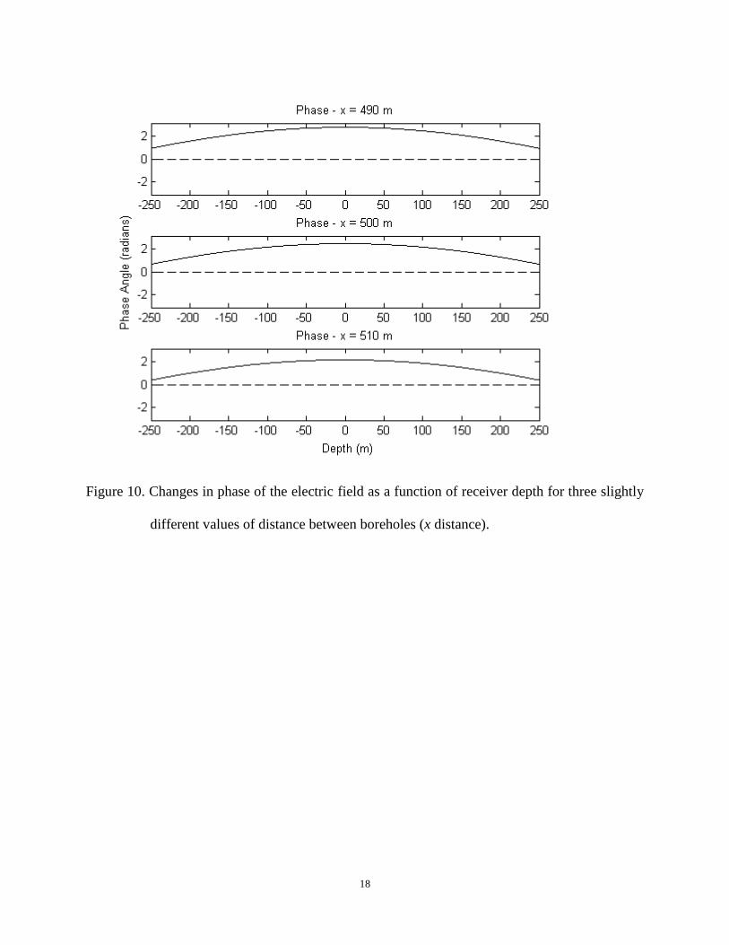
Figure 10. Changes in phase of the electric field as a function of receiver depth for three slightly
different values of distance between boreholes (x distance). ........................................................ 18
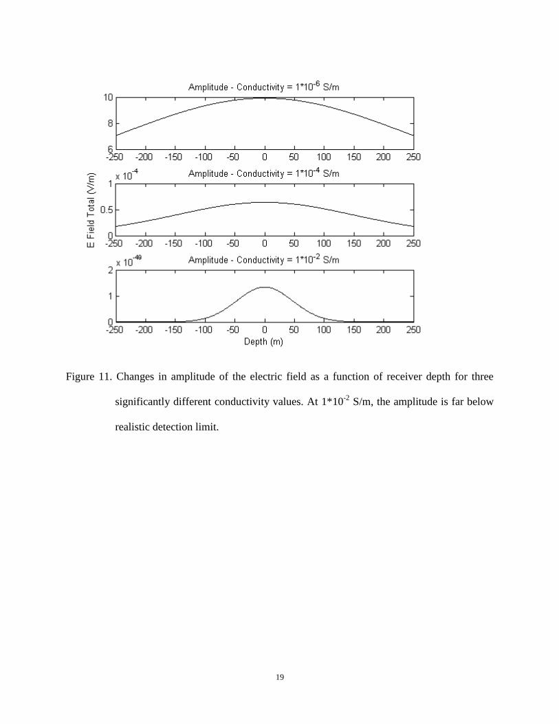
Figure 11. Changes in amplitude of the electric field as a function of receiver depth for three
significantly different conductivity values. At 1*10-2
S/m, the amplitude is far below realistic
detection limit. .............................................................................................................................. 19
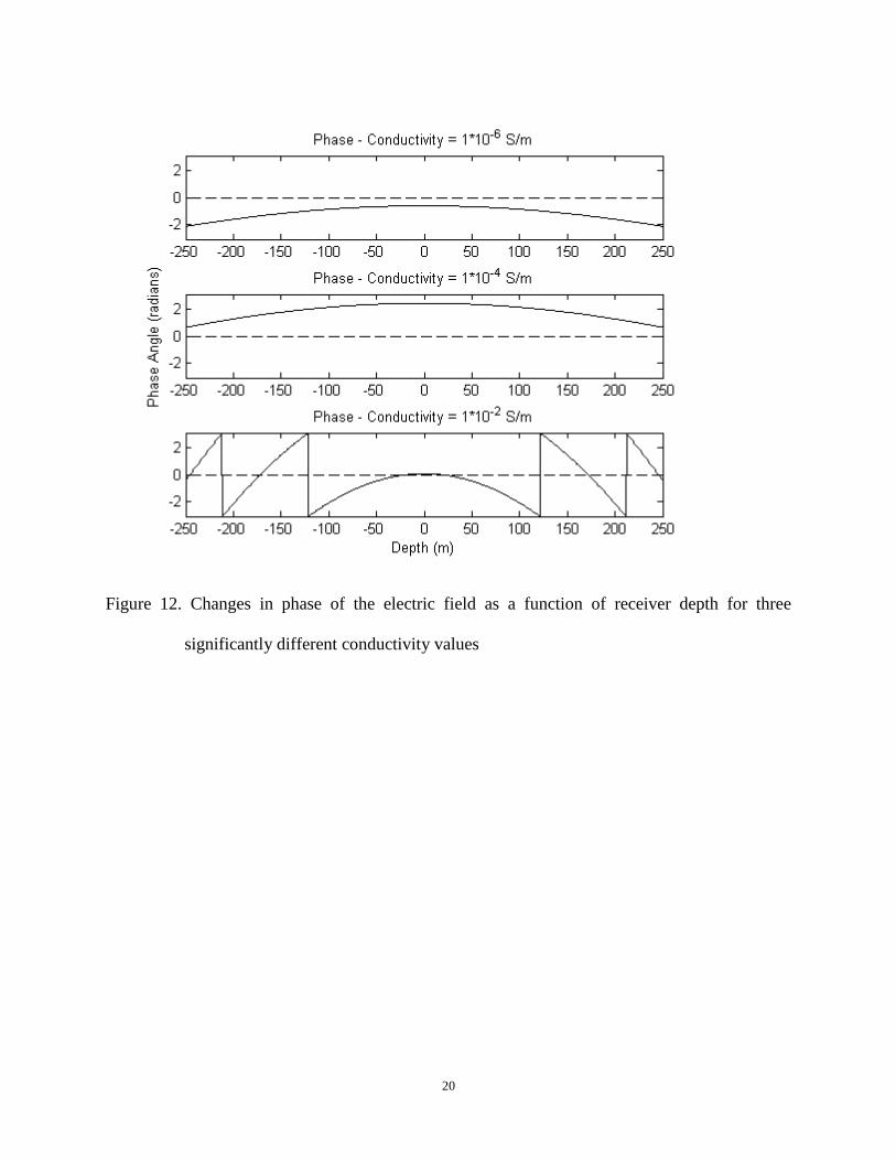
Figure 12. Changes in phase of the electric field as a function of receiver depth for three
significantly different conductivity values.................................................................................... 20
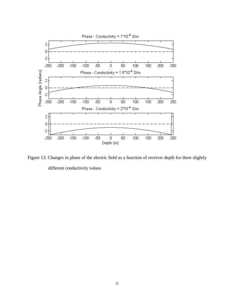
Figure 13. Changes in phase of the electric field as a function of receiver depth for three slightly
different conductivity values ......................................................................................................... 21
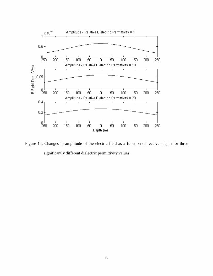
Figure 14. Changes in amplitude of the electric field as a function of receiver depth for three
significantly different dielectric permittivity values. .................................................................... 22
Figure 15. Changes in phase of the electric field as a function of receiver depth for three
significantly different dielectric permittivity values. .................................................................... 23
ix
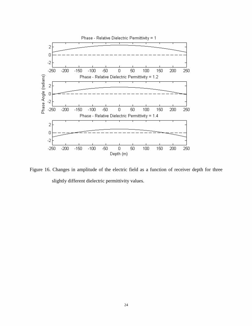
Figure 16. Changes in amplitude of the electric field as a function of receiver depth for three
slightly different dielectric permittivity values. ............................................................................ 24
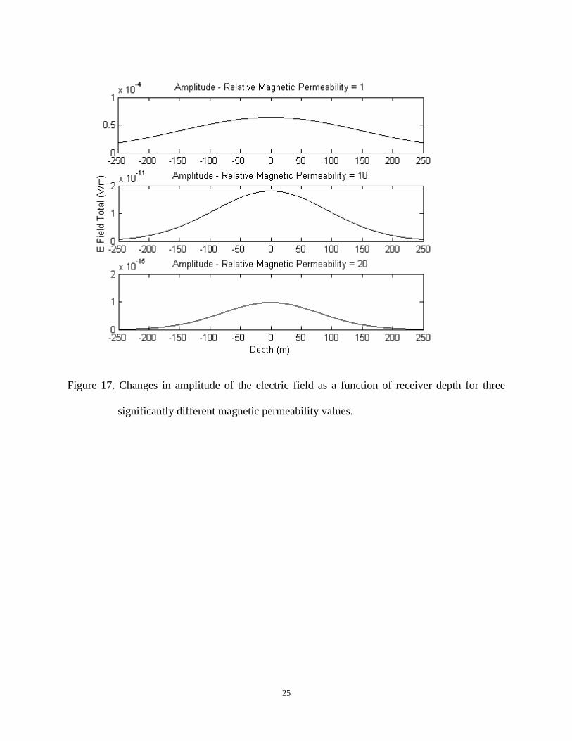
Figure 17. Changes in amplitude of the electric field as a function of receiver depth for three
significantly different magnetic permeability values. ................................................................... 25
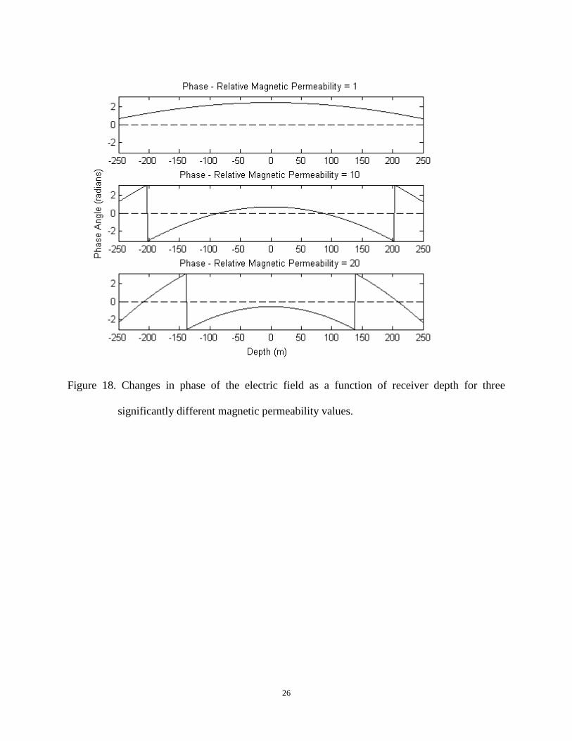
Figure 18. Changes in phase of the electric field as a function of receiver depth for three
significantly different magnetic permeability values. ................................................................... 26
Figure 19. Changes in amplitude of the electric field as a function of receiver depth for three
slightly different magnetic permeability values. ........................................................................... 27
Figure 20: The peak amplitudes of four frequencies as a function of the distance between
boreholes. This is for a parallel borehole system, with a conductivity of 10-4
S/m. ..................... 30
Figure 21: The peak amplitudes of four frequencies as a function of the conductivity. This is for
a parallel borehole system, with the distance between boreholes set to 500m. ............................ 31
Figure 22. The peak amplitudes of four frequencies as a function of the distance between
boreholes. This is for a parallel borehole system, with a conductivity of 10-5
S/m. ..................... 32
Figure 23. Conductivity versus x distance plot, showing the frequency in each region with the
greatest amplitude at that combination of values for the two parameters. A sensitivity of 25% is
also added, such that any other frequency that is within 25% of the greatest amplitude will also
be shown. ...................................................................................................................................... 33
Figure 24. Conductivity versus x distance plot, showing the frequency in each region whose
amplitude exceeds its roughly estimated noise level at that combination of values for the two
parameters. .................................................................................................................................... 34
Figure 25. The two angled borehole geometries used for the simulations in Figure 26. .............. 35
x
Figure 26. (top) A comparison of the amplitudes between a parallel borehole system (solid line),
a system with the receiver borehole at an angle of 20 degrees (dash line), and a system with the
transmitter borehole at an angle of 20 degrees (dash-dot line). .................................................... 36
Figure 27. The peak amplitude and peak position as a function of the borehole angle. The peak
position is measured with respect to the position directly across from the transmitter where the
zero degree peak occurs. This is for a 10-4
S/m whole space with the distance between boreholes
set to 500m. ................................................................................................................................... 37
Figure 28. The 625 kHz resistivity tomogram. ............................................................................. 40
Figure 29. The 1250 kHz resistivity tomogram. ........................................................................... 41
Figure 30. The 2500 kHz resistivity tomogram. ........................................................................... 42
Figure 31. The modelling program recreation of the geometric system in the Drury RIM data
collection. ...................................................................................................................................... 44
Figure 32. Model and real data comparisons, with the transmitter at -275 m in borehole DR-160,
frequency = 625 kHz. The model conductivity is set to 2.1*10-3
S/m. ........................................ 46
Figure 33. Model and real data comparisons, with the transmitter at -275 m in borehole DR-160,
frequency = 1250 kHz. The model conductivity is set to 3*10-3
S/m. ......................................... 47
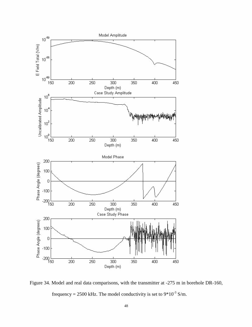
Figure 34. Model and real data comparisons, with the transmitter at -275 m in borehole DR-160,
frequency = 2500 kHz. The model conductivity is set to 9*10-3
S/m. ......................................... 48
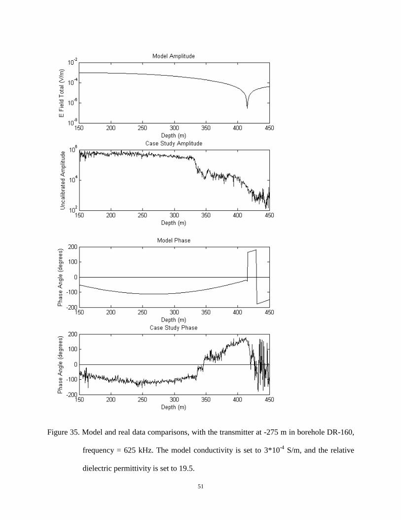
Figure 35. Model and real data comparisons, with the transmitter at -275 m in borehole DR-160,
frequency = 625 kHz. The model conductivity is set to 3*10-4
S/m, and the relative dielectric
permittivity is set to 19.5. ............................................................................................................. 51
xi
Figure 36. Model and real data comparisons, with the transmitter at -275 m in borehole DR-160,
frequency = 1250 kHz. The model conductivity is set to 3*10-4
S/m, and the relative dielectric
permittivity is set to 17.3. ............................................................................................................. 52
Figure 37. Model and real data comparisons, with the transmitter at -275 m in borehole DR-160,
frequency = 2500 kHz. The model conductivity is set to 3*10-4
S/m, and the relative dielectric
permittivity is set to 18. ................................................................................................................ 53
Figure 38. An example of the Python GUI. .................................................................................. 55
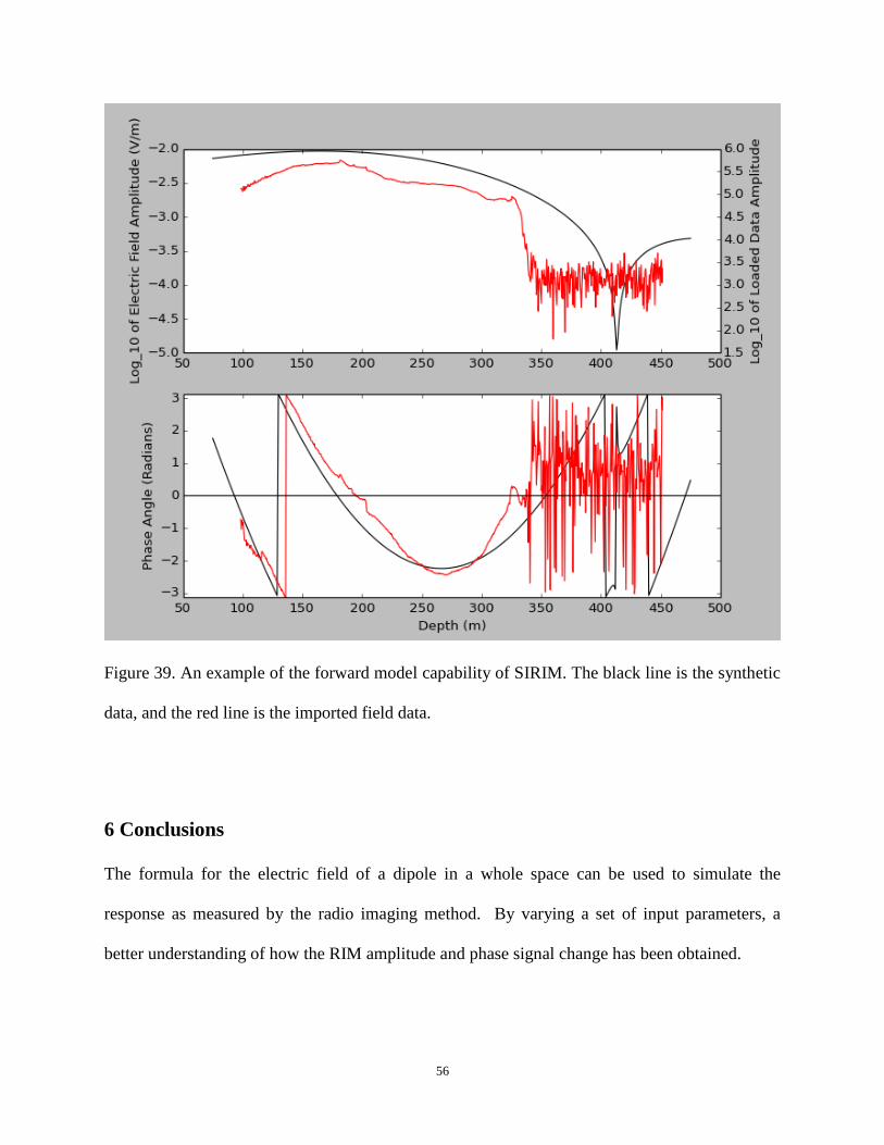
Figure 39. An example of the forward model capability of SIRIM. The black line is the synthetic
data, and the red line is the imported field data. ........................................................................... 56
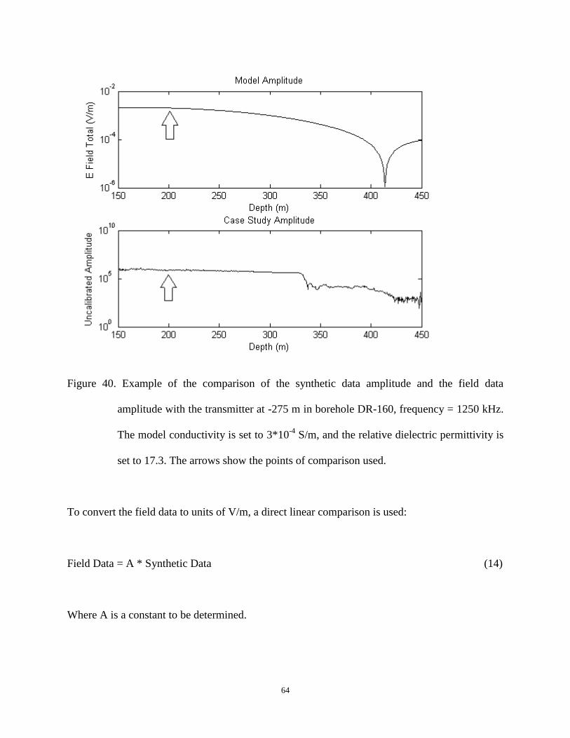
Figure 40. Example of the comparison of the synthetic data amplitude and the field data
amplitude with the transmitter at -275 m in borehole DR-160, frequency = 1250 kHz. The model
conductivity is set to 3*10-4
S/m, and the relative dielectric permittivity is set to 17.3. The arrows
show the points of comparison used. ............................................................................................ 64
Figure 41. Example of the noise level estimate, using the 1250 kHz data with the transmitter at -
275 m in borehole DR-160. Noise here is at approximately 103 uncalibrated units. .................... 65
Figure 42. The measured real and imaginary components for the synthetic data from Figure 32.
....................................................................................................................................................... 67
Figure 43. The mesured z and x components for the synthetic data from Figure 32. ................... 68
Figure 44. The peak amplitudes of four frequencies as a function of the relative dielectric
permittivity. This is for a parallel borehole system, with the distance between boreholes set to
500 m, and a conductivity of 10-4
S/m. ......................................................................................... 70
xii
Figure 45. The peak amplitudes of four frequencies as a function of the relative dielectric
permittivity. This is for a parallel borehole system, with the distance between boreholes set to
500 m, and a conductivity of 10-5
S/m. ......................................................................................... 71
Figure 46. The peak amplitudes of four frequencies as a function of the relative dielectric
permittivity. This is for a parallel borehole system, with the distance between boreholes set to
500 m, and a conductivity of 10-3
S/m. ......................................................................................... 72
1
1 Introduction
The radio imaging method (RIM) is a tomographic geophysical method that can be used to map
electromagnetic properties in areas of interest between boreholes. Developed for the coal mining
industry (Stolarczyk and Fry, 1986), RIM has since been applied with some success in several
other areas, including mineral exploration and delineation (Thomson et al., 1992; Fullagar et al.,
2000), and characterization of rock (Zhou and Fullagar, 2001; Korpisalo and Heikkinen, 2014).
RIM is effective at locating areas of high conductivity which can be indicative of sulphide-
bearing zones. The conductive medium causes the electromagnetic (EM) radiation emitted by the
transmitter to attenuate, while resistive zones allow the radiation to propagate without
attenuation. Zones of strong attenuation indicate an area of potential interest (Zhou et al., 1998;
Stevens et al., 2000).
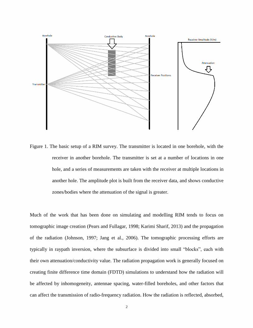
RIM surveys are conducted by placing a transmitter antenna down a borehole, and at a number
of set locations, radio-frequency radiation is emitted (Figure 1). This is received by an antenna at
multiple locations in another borehole, and the resulting signals can be used to determine
features of the material between the two boreholes. In the mining industry the results can be used
to focus the drilling where potential targets may be. Alternatively, if there is confidence in the
RIM results, further drilling could be minimized or avoided (Mutton, 2000).
2
Figure 1. The basic setup of a RIM survey. The transmitter is located in one borehole, with the
receiver in another borehole. The transmitter is set at a number of locations in one
hole, and a series of measurements are taken with the receiver at multiple locations in
another hole. The amplitude plot is built from the receiver data, and shows conductive
zones/bodies where the attenuation of the signal is greater.
Much of the work that has been done on simulating and modelling RIM tends to focus on
tomographic image creation (Pears and Fullagar, 1998; Karimi Sharif, 2013) and the propagation
of the radiation (Johnson, 1997; Jang et al., 2006). The tomographic processing efforts are
typically in raypath inversion, where the subsurface is divided into small “blocks”, each with
their own attenuation/conductivity value. The radiation propagation work is generally focused on
creating finite difference time domain (FDTD) simulations to understand how the radiation will
be affected by inhomogeneity, antennae spacing, water-filled boreholes, and other factors that
can affect the transmission of radio-frequency radiation. How the radiation is reflected, absorbed,
3
and re-emitted is important to understand in RIM and assists in interpretation of RIM data.
However, there is less research in radiation propagation done in the context of the received
signal, and the effects of the physical and geometric parameters of the system that affect RIM.
As such, this research was carried out with the goal of better understanding the electric field that
would be measured at the receivers, based on the parameters of the whole-space model and the
system geometry.
The representation of the transmitter as a single infinitesimal dipole is an assumption used
(Holliger et al., 2001) in much of RIM research. The validity of this approximation was
investigated by constructing a larger dipole of multiple infinitesimal dipoles.
The borehole separation, conductivity, dielectric permittivity, magnetic susceptibility, frequency
of the transmitter, and angles of the boreholes were all parameters which were analyzed to
understand their effects on the amplitude and phase. Understanding how the signal changes when
a single one of these system parameters is varied will allow an understanding of how each of the
parameters can affect data. Furthermore, the complex interaction of how each parameter may
accentuate or reduce the effect of another parameter was investigated.
This knowledge will allow more confidence in results, as well as assist in interpretations of an
area that is being surveyed by RIM. Additionally, this research has led to the creation of basic
forward model software specifically for RIM survey data.
4
2 Method
To investigate the signal of RIM data, a whole-space modelling program was created in Matlab®
using the formulation of Ward and Hohmann (1987). The program simulates the transmitter as
an electric dipole in a homogeneous whole space, and calculates the resulting electric field that
would be measured in a receiver borehole, as a function of the parameters of the whole space and
the system geometry (Figure 2). By varying parameters of the model, it is possible to gain an
understanding of how the signal changes, which can ultimately assist in creating more accurate
inversions and interpretations.
The mathematical formula describing the electric field E of a z-directed electric dipole associated
with this model is Equation 1 (adapted from Ward and Hohmann, 1987, p.173, and additional
description from Zhou and Fullagar, 2001):
𝐄 =𝐼 𝑑𝑠
4𝜋𝜎𝑟3 𝑒−𝑖𝑘𝑟 [(𝑧2
𝑟2 𝒖𝒛 +𝑧𝑦
𝑟2 𝒖𝒚 +𝑧𝑥
𝑟2 𝒖𝒙) (−𝑘2𝑟2 + 3𝑖𝑘𝑟 + 3) + (𝑘2𝑟2 − 𝑖𝑘𝑟 − 1)𝒖𝒛], (1)
where:
𝑟 = √𝑥2 + 𝑦2 + 𝑧2, (2)
𝑘 = 𝛼 − 𝑖𝛽, is the complex wavenumber, (3)
𝛼 = 𝜔 {𝜇𝜀
2[(1 +
𝜎2
𝜀2𝜔2)1
2⁄
+ 1]}
12⁄
, is the wavenumber/phase coefficient (4)
and
𝛽 = 𝜔 {𝜇𝜀
2[(1 +
𝜎2
𝜀2𝜔2)1
2⁄
− 1]}
12⁄
, is the attenuation rate/absorption coefficient (5)
5
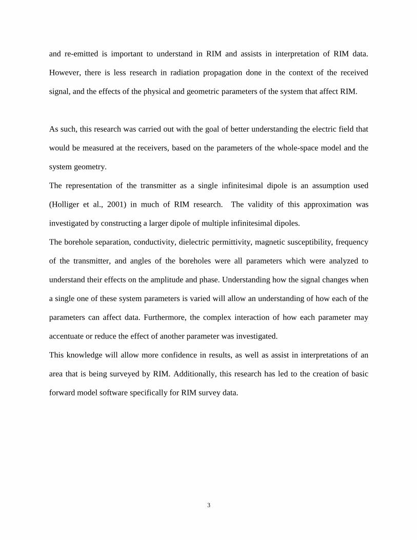
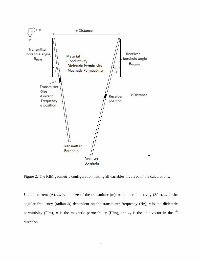
Figure 2: The RIM geometric configuration, listing all variables involved in the calculations.
I is the current (A), ds is the size of the transmitter (m), σ is the conductivity (S/m), ω is the
angular frequency (radians/s) dependent on the transmitter frequency (Hz), ɛ is the dielectric
permittivity (F/m), µ is the magnetic permeability (H/m), and ui is the unit vector in the ith
direction.
6
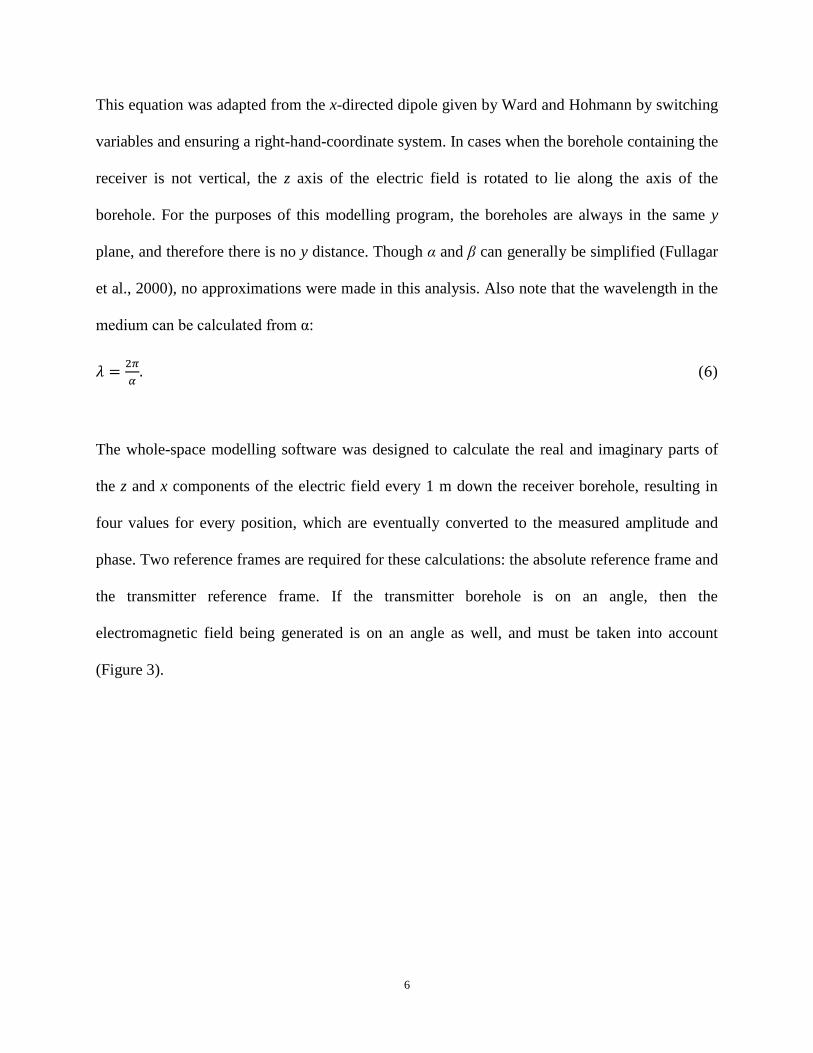
This equation was adapted from the x-directed dipole given by Ward and Hohmann by switching
variables and ensuring a right-hand-coordinate system. In cases when the borehole containing the
receiver is not vertical, the z axis of the electric field is rotated to lie along the axis of the
borehole. For the purposes of this modelling program, the boreholes are always in the same y
plane, and therefore there is no y distance. Though α and β can generally be simplified (Fullagar
et al., 2000), no approximations were made in this analysis. Also note that the wavelength in the
medium can be calculated from α:
𝜆 =2𝜋
𝛼. (6)
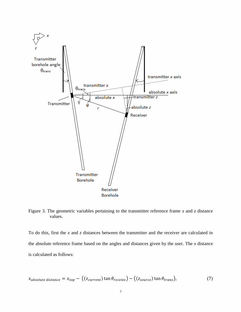
The whole-space modelling software was designed to calculate the real and imaginary parts of
the z and x components of the electric field every 1 m down the receiver borehole, resulting in
four values for every position, which are eventually converted to the measured amplitude and
phase. Two reference frames are required for these calculations: the absolute reference frame and
the transmitter reference frame. If the transmitter borehole is on an angle, then the
electromagnetic field being generated is on an angle as well, and must be taken into account
(Figure 3).
7
Figure 3. The geometric variables pertaining to the transmitter reference frame x and z distance
values.
To do this, first the x and z distances between the transmitter and the receiver are calculated in
the absolute reference frame based on the angles and distances given by the user. The x distance
is calculated as follows:
𝑥𝑎𝑏𝑠𝑜𝑙𝑢𝑡𝑒 𝑑𝑖𝑠𝑡𝑎𝑛𝑐𝑒 = 𝑥𝑡𝑜𝑝 − ((𝑧𝑐𝑢𝑟𝑟𝑒𝑛𝑡) tan 𝜃𝑟𝑒𝑐𝑒𝑖𝑣𝑒) − ((𝑧𝑠𝑜𝑢𝑟𝑐𝑒) tan 𝜃𝑡𝑟𝑎𝑛𝑠), (7)
8
xtop is the x distance between boreholes at the top of the model, zcurrent is the current receiver z
position being calculated, zsource is the z position of the transmitter vertically, θtrans is the angle of
the transmitter borehole with respect to the vertical, and θreceive is the angle of the receiver
borehole with respect to the vertical. For both angles, a positive angle specifies the borehole
being rotated towards the center of the system (bottom of the hole rotated in), while a negative
angle specifies the borehole being rotated away from the center of the system (rotated out). In
other words, for the right borehole, a positive angle is a clockwise rotation and for the left it is
counter-clockwise. The transmitter is always assumed to be on the left side.
The depth of the receiver is measured relative to the position of the transmitter, with negative
depths referring to depths above the transmitter, in the ground reference system:
𝑧𝑎𝑏𝑠𝑜𝑙𝑢𝑡𝑒 𝑑𝑖𝑠𝑡𝑎𝑛𝑐𝑒 = 𝑧𝑐𝑢𝑟𝑟𝑒𝑛𝑡 − 𝑧𝑠𝑜𝑢𝑟𝑐𝑒, (8)
Using the x and z distances, the angle γ between the direct path from transmitter to receiver
(referred to as r) and the absolute x axis is given by:
𝛾 = tan−1 (𝑧𝑎𝑏𝑠𝑜𝑙𝑢𝑡𝑒 𝑑𝑖𝑠𝑡𝑎𝑛𝑐𝑒
𝑥𝑎𝑏𝑠𝑜𝑙𝑢𝑡𝑒 𝑑𝑖𝑠𝑡𝑎𝑛𝑐𝑒), (9)
and, the angle between r and the x axis in the transmitter reference frame is given by:
𝜙 = 𝛾 + 𝜃𝑡𝑟𝑎𝑛𝑠. (10)
9
Having defined ϕ, the transmitter reference frame x and z values are simply:
𝑥𝑡𝑟𝑎𝑛𝑠 𝑑𝑖𝑠𝑡𝑎𝑛𝑐𝑒 = 𝑟 cos 𝜙, (11)
𝑧𝑡𝑟𝑎𝑛𝑠 𝑑𝑖𝑠𝑡𝑎𝑛𝑐𝑒 = 𝑟 sin 𝜙, (12)
The component of the electric field that would be measured by a sensor oriented along the
receiver borehole is then calculated, based on the angles of the boreholes in degrees:
𝐸𝑐𝑢𝑟𝑟𝑒𝑛𝑡 = (cos(𝜃𝑡𝑟𝑎𝑛𝑠 + 𝜃𝑟𝑒𝑐𝑒𝑖𝑣𝑒))𝐸𝑐𝑢𝑟𝑟𝑒𝑛𝑡,𝑧 + (cos(90˚ − 𝜃𝑡𝑟𝑎𝑛𝑠 + 𝜃𝑟𝑒𝑐𝑒𝑖𝑣𝑒))𝐸𝑐𝑢𝑟𝑟𝑒𝑛𝑡,𝑥, (13)
This is done for both real and imaginary components, and finally the total amplitude and phase
angle are calculated and plotted (Figure 4).
10
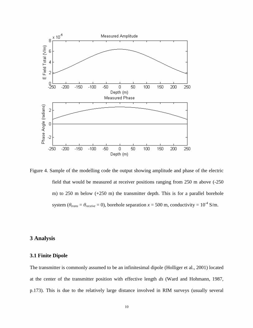
Figure 4. Sample of the modelling code the output showing amplitude and phase of the electric
field that would be measured at receiver positions ranging from 250 m above (-250
m) to 250 m below (+250 m) the transmitter depth. This is for a parallel borehole
system (θtrans = θreceive = 0), borehole separation x = 500 m, conductivity = 10-4
S/m.
3 Analysis
3.1 Finite Dipole
The transmitter is commonly assumed to be an infinitesimal dipole (Holliger et al., 2001) located
at the center of the transmitter position with effective length ds (Ward and Hohmann, 1987,
p.173). This is due to the relatively large distance involved in RIM surveys (usually several
11
hundred metres), compared to the size of the transmitter dipole (generally a few tens of metres).
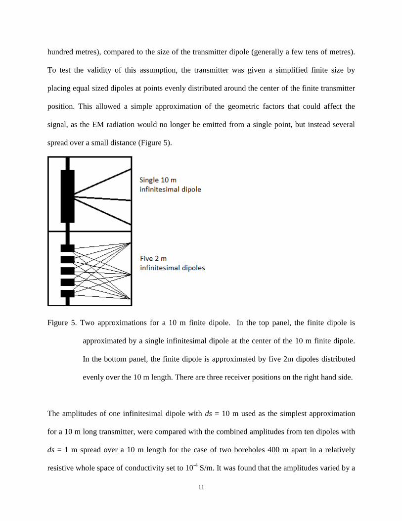
To test the validity of this assumption, the transmitter was given a simplified finite size by
placing equal sized dipoles at points evenly distributed around the center of the finite transmitter
position. This allowed a simple approximation of the geometric factors that could affect the
signal, as the EM radiation would no longer be emitted from a single point, but instead several
spread over a small distance (Figure 5).
Figure 5. Two approximations for a 10 m finite dipole. In the top panel, the finite dipole is
approximated by a single infinitesimal dipole at the center of the 10 m finite dipole.
In the bottom panel, the finite dipole is approximated by five 2m dipoles distributed
evenly over the 10 m length. There are three receiver positions on the right hand side.
The amplitudes of one infinitesimal dipole with ds = 10 m used as the simplest approximation
for a 10 m long transmitter, were compared with the combined amplitudes from ten dipoles with
ds = 1 m spread over a 10 m length for the case of two boreholes 400 m apart in a relatively
resistive whole space of conductivity set to 10-4
S/m. It was found that the amplitudes varied by a
12
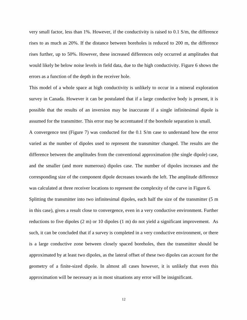
very small factor, less than 1%. However, if the conductivity is raised to 0.1 S/m, the difference
rises to as much as 20%. If the distance between boreholes is reduced to 200 m, the difference
rises further, up to 50%. However, these increased differences only occurred at amplitudes that
would likely be below noise levels in field data, due to the high conductivity. Figure 6 shows the
errors as a function of the depth in the receiver hole.
This model of a whole space at high conductivity is unlikely to occur in a mineral exploration
survey in Canada. However it can be postulated that if a large conductive body is present, it is
possible that the results of an inversion may be inaccurate if a single infinitesimal dipole is
assumed for the transmitter. This error may be accentuated if the borehole separation is small.
A convergence test (Figure 7) was conducted for the 0.1 S/m case to understand how the error
varied as the number of dipoles used to represent the transmitter changed. The results are the
difference between the amplitudes from the conventional approximation (the single dipole) case,
and the smaller (and more numerous) dipoles case. The number of dipoles increases and the
corresponding size of the component dipole decreases towards the left. The amplitude difference
was calculated at three receiver locations to represent the complexity of the curve in Figure 6.
Splitting the transmitter into two infinitesimal dipoles, each half the size of the transmitter (5 m
in this case), gives a result close to convergence, even in a very conductive environment. Further
reductions to five dipoles (2 m) or 10 dipoles (1 m) do not yield a significant improvement. As
such, it can be concluded that if a survey is completed in a very conductive environment, or there
is a large conductive zone between closely spaced boreholes, then the transmitter should be
approximated by at least two dipoles, as the lateral offset of these two dipoles can account for the
geometry of a finite-sized dipole. In almost all cases however, it is unlikely that even this
approximation will be necessary as in most situations any error will be insignificant.
13
Figure 6: A plot depicting the difference in magnitude between a transmitter calculated as a
single 10 m dipole, and a transmitter calculated as ten evenly spaced 1 m dipoles.
Each curve is for a different borehole separation and/or whole-space conductivity.
The cusps in the dashed and dotted cases represent a switch in the sign of the
magnitude difference, as the amplitudes begin as greater than the 10 m dipole case’s
amplitude, before falling in magnitudes to less than that of the 10 m dipole case’s
amplitude.
14
Figure 7: A convergence test for the finite dipole transmitter investigation, where the vertical
boreholes are separated by 400 m, the conductivity is 10-1
S/m and the transmitter
dipole is 10 m. The component size was reduced until approximate convergence was
reached. The y-axis shows the difference in amplitude between each size and the 10
m component size. It is calculated for three different points along the receiver
borehole, 250 m above the transmitter, 150 m above the transmitter, and 50 m above
the transmitter.
15
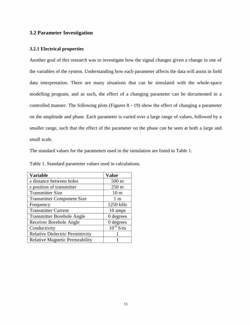
3.2 Parameter Investigation
3.2.1 Electrical properties
Another goal of this research was to investigate how the signal changes given a change in one of
the variables of the system. Understanding how each parameter affects the data will assist in field
data interpretation. There are many situations that can be simulated with the whole-space
modelling program, and as such, the effect of a changing parameter can be documented in a
controlled manner. The following plots (Figures 8 - 19) show the effect of changing a parameter
on the amplitude and phase. Each parameter is varied over a large range of values, followed by a
smaller range, such that the effect of the parameter on the phase can be seen at both a large and
small scale.
The standard values for the parameters used in the simulation are listed in Table 1.
Table 1. Standard parameter values used in calculations.
Variable Value
x distance between holes 500 m
z position of transmitter 250 m
Transmitter Size 10 m
Transmitter Component Size 1 m
Frequency 1250 kHz
Transmitter Current 10 amps
Transmitter Borehole Angle 0 degrees
Receiver Borehole Angle 0 degrees
Conductivity 10-4
S/m
Relative Dielectric Permittivity 1
Relative Magnetic Permeability 1
16
Figure 8. Changes in amplitude of the electric field as a function of receiver depth for three
significantly different values of distance between boreholes (x distance).
17
Figure 9. Changes in phase of the electric field as a function of receiver depth for three
significantly different values of distance between boreholes (x distance).
18
Figure 10. Changes in phase of the electric field as a function of receiver depth for three slightly
different values of distance between boreholes (x distance).
19
Figure 11. Changes in amplitude of the electric field as a function of receiver depth for three
significantly different conductivity values. At 1*10-2
S/m, the amplitude is far below
realistic detection limit.
20
Figure 12. Changes in phase of the electric field as a function of receiver depth for three
significantly different conductivity values
21
Figure 13. Changes in phase of the electric field as a function of receiver depth for three slightly
different conductivity values
22
Figure 14. Changes in amplitude of the electric field as a function of receiver depth for three
significantly different dielectric permittivity values.

23
Figure 15. Changes in phase of the electric field as a function of receiver depth for three
significantly different dielectric permittivity values.
24
Figure 16. Changes in amplitude of the electric field as a function of receiver depth for three
slightly different dielectric permittivity values.
25
Figure 17. Changes in amplitude of the electric field as a function of receiver depth for three
significantly different magnetic permeability values.
26
Figure 18. Changes in phase of the electric field as a function of receiver depth for three
significantly different magnetic permeability values.
27
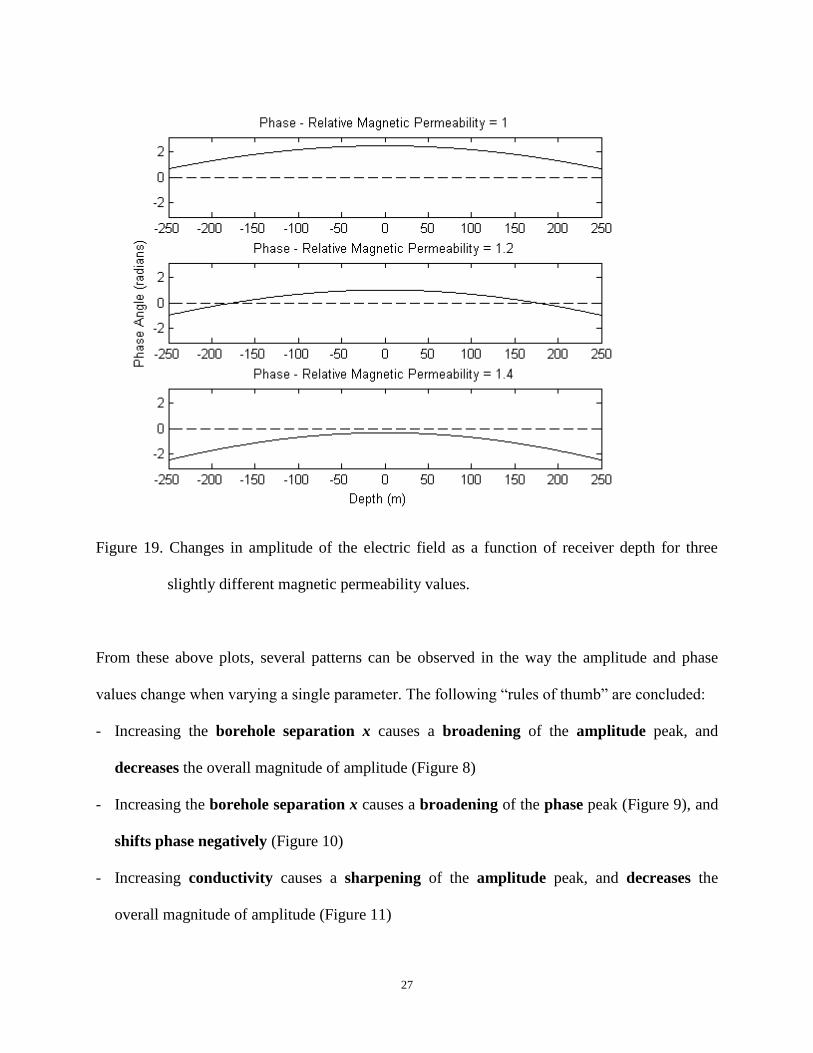
Figure 19. Changes in amplitude of the electric field as a function of receiver depth for three
slightly different magnetic permeability values.
From these above plots, several patterns can be observed in the way the amplitude and phase
values change when varying a single parameter. The following “rules of thumb” are concluded:
- Increasing the borehole separation x causes a broadening of the amplitude peak, and
decreases the overall magnitude of amplitude (Figure 8)
- Increasing the borehole separation x causes a broadening of the phase peak (Figure 9), and
shifts phase negatively (Figure 10)
- Increasing conductivity causes a sharpening of the amplitude peak, and decreases the
overall magnitude of amplitude (Figure 11)
28
- Increasing conductivity causes a sharpening of the phase peak (Figure 12), and shifts phase
negatively (Figure 13)
- Increasing the dielectric permittivity causes a small broadening of the shape of the
amplitude peak, and increases the overall magnitude of the amplitude (Figure 14)
- Increasing dielectric permittivity causes a sharpening of the phase peak (Figure 15), and
shifts phase negatively (Figure 16)
- Increasing magnetic permeability causes a sharpening of the amplitude peak, and
decreases the overall magnitude of amplitude (Figure 17)
- Increasing magnetic permeability causes a sharpening of the phase peak (Figure 18), and
shifts phase negatively (Figure 19)
These rules are summarized in Table 2 below.
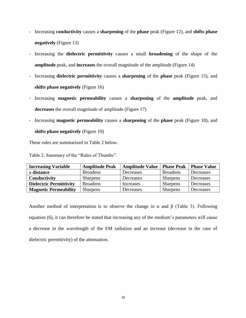
Table 2. Summary of the “Rules of Thumbs”.
Increasing Variable Amplitude Peak Amplitude Value Phase Peak Phase Value
x distance Broadens Decreases Broadens Decreases
Conductivity Sharpens Decreases Sharpens Decreases
Dielectric Permittivity Broadens Increases Sharpens Decreases
Magnetic Permeability Sharpens Decreases Sharpens Decreases
Another method of interpretation is to observe the change in α and β (Table 3). Following
equation (6), it can therefore be stated that increasing any of the medium’s parameters will cause
a decrease in the wavelength of the EM radiation and an increase (decrease in the case of
dielectric permittivity) of the attenuation.
29
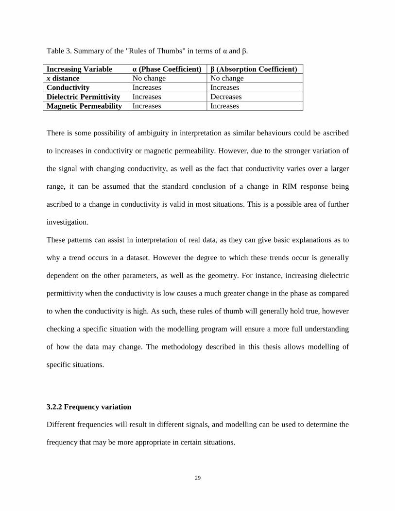
Table 3. Summary of the "Rules of Thumbs" in terms of α and β.
Increasing Variable α (Phase Coefficient) β (Absorption Coefficient)
x distance No change No change
Conductivity Increases Increases
Dielectric Permittivity Increases Decreases
Magnetic Permeability Increases Increases
There is some possibility of ambiguity in interpretation as similar behaviours could be ascribed
to increases in conductivity or magnetic permeability. However, due to the stronger variation of
the signal with changing conductivity, as well as the fact that conductivity varies over a larger
range, it can be assumed that the standard conclusion of a change in RIM response being
ascribed to a change in conductivity is valid in most situations. This is a possible area of further
investigation.
These patterns can assist in interpretation of real data, as they can give basic explanations as to
why a trend occurs in a dataset. However the degree to which these trends occur is generally
dependent on the other parameters, as well as the geometry. For instance, increasing dielectric
permittivity when the conductivity is low causes a much greater change in the phase as compared
to when the conductivity is high. As such, these rules of thumb will generally hold true, however
checking a specific situation with the modelling program will ensure a more full understanding
of how the data may change. The methodology described in this thesis allows modelling of
specific situations.
3.2.2 Frequency variation
Different frequencies will result in different signals, and modelling can be used to determine the
frequency that may be more appropriate in certain situations.
30
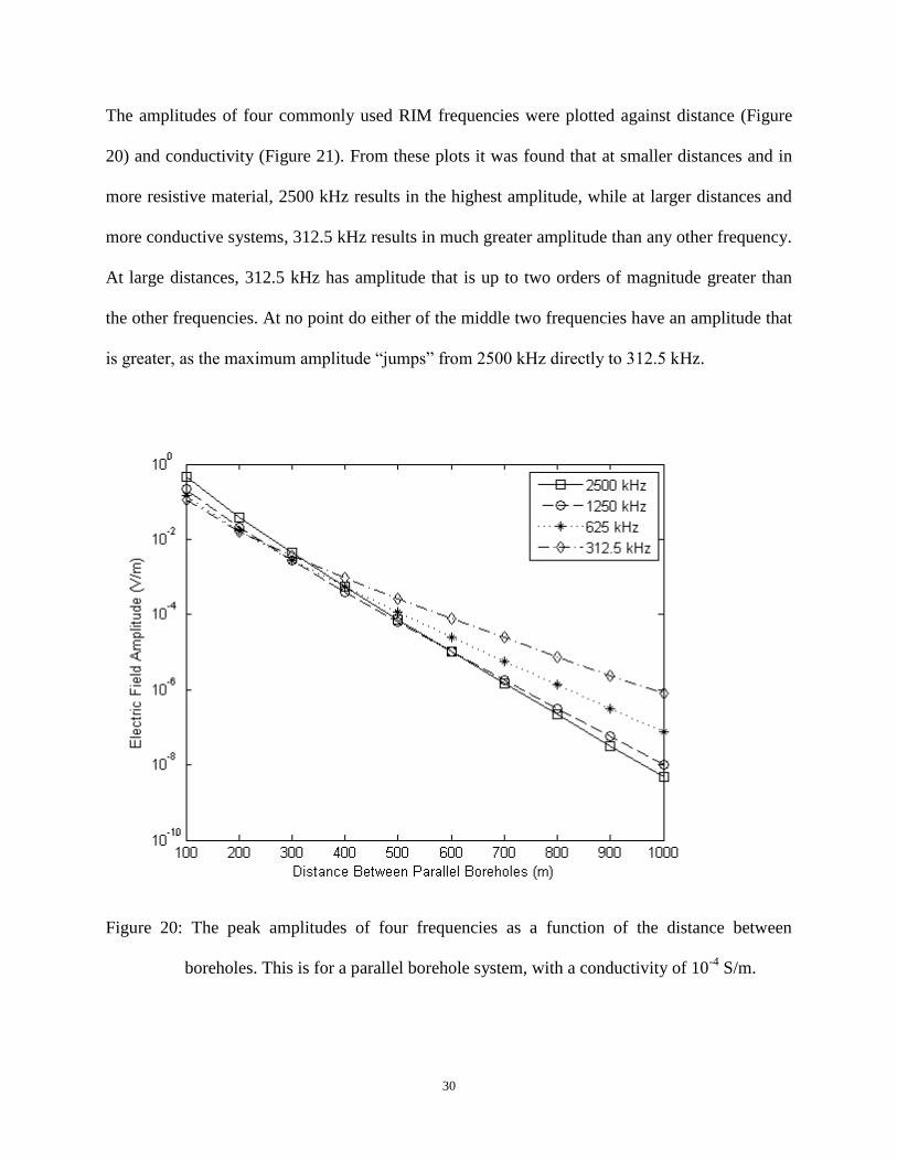
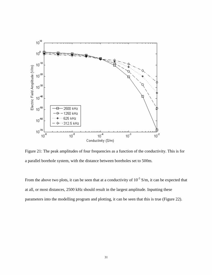
The amplitudes of four commonly used RIM frequencies were plotted against distance (Figure
20) and conductivity (Figure 21). From these plots it was found that at smaller distances and in
more resistive material, 2500 kHz results in the highest amplitude, while at larger distances and
more conductive systems, 312.5 kHz results in much greater amplitude than any other frequency.
At large distances, 312.5 kHz has amplitude that is up to two orders of magnitude greater than
the other frequencies. At no point do either of the middle two frequencies have an amplitude that
is greater, as the maximum amplitude “jumps” from 2500 kHz directly to 312.5 kHz.
Figure 20: The peak amplitudes of four frequencies as a function of the distance between
boreholes. This is for a parallel borehole system, with a conductivity of 10-4
S/m.
31
Figure 21: The peak amplitudes of four frequencies as a function of the conductivity. This is for
a parallel borehole system, with the distance between boreholes set to 500m.
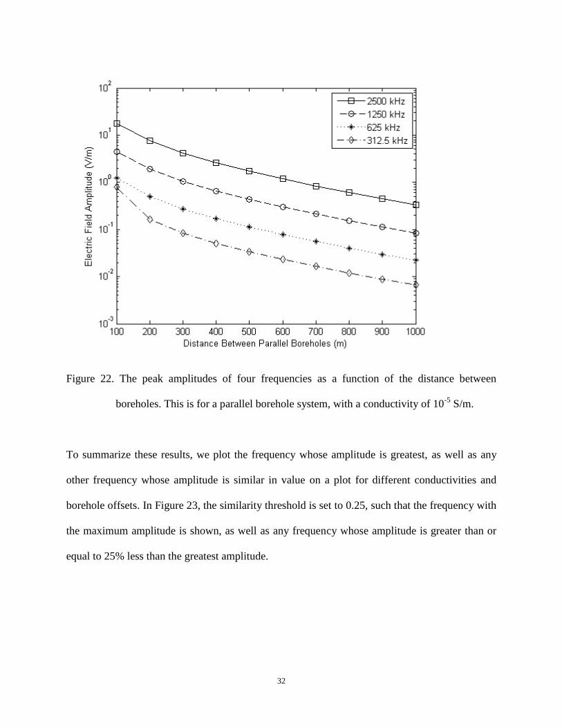
From the above two plots, it can be seen that at a conductivity of 10-5
S/m, it can be expected that
at all, or most distances, 2500 kHz should result in the largest amplitude. Inputting these
parameters into the modelling program and plotting, it can be seen that this is true (Figure 22).
32
Figure 22. The peak amplitudes of four frequencies as a function of the distance between
boreholes. This is for a parallel borehole system, with a conductivity of 10-5
S/m.
To summarize these results, we plot the frequency whose amplitude is greatest, as well as any
other frequency whose amplitude is similar in value on a plot for different conductivities and
borehole offsets. In Figure 23, the similarity threshold is set to 0.25, such that the frequency with
the maximum amplitude is shown, as well as any frequency whose amplitude is greater than or
equal to 25% less than the greatest amplitude.
33
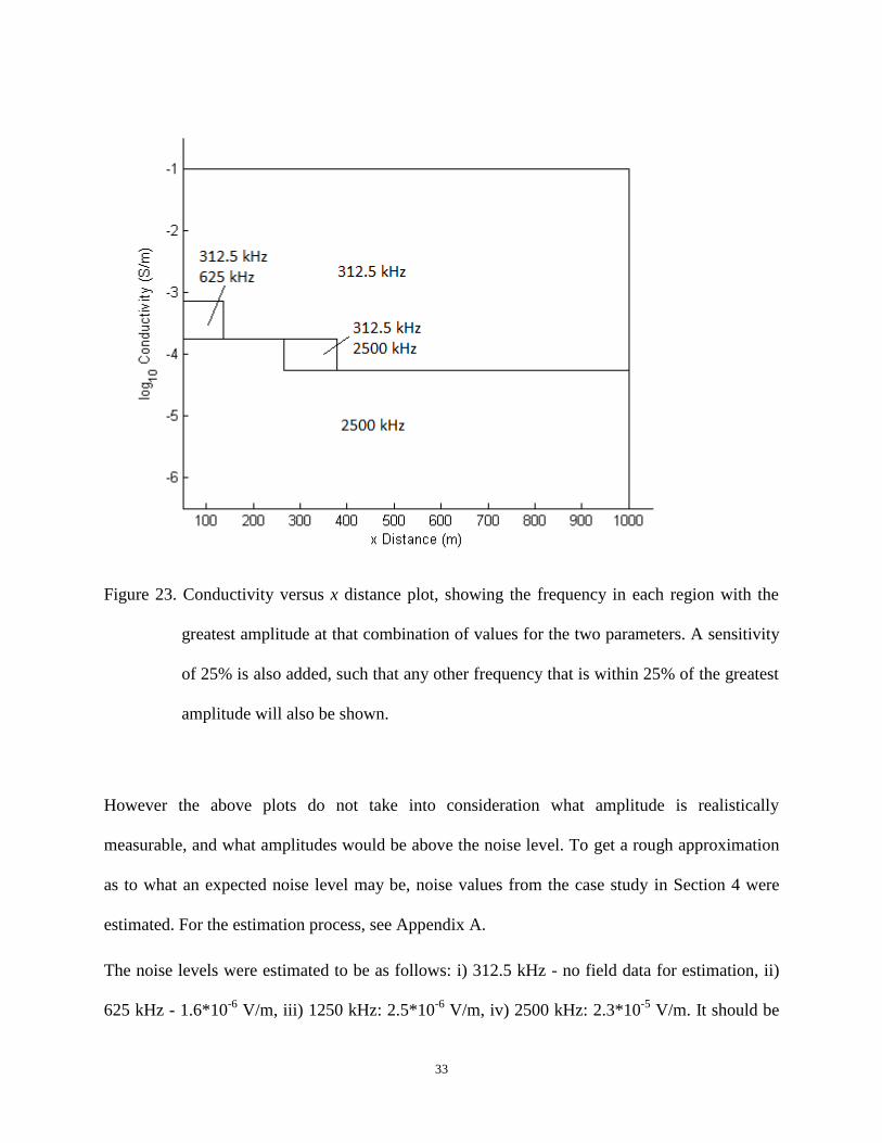
Figure 23. Conductivity versus x distance plot, showing the frequency in each region with the
greatest amplitude at that combination of values for the two parameters. A sensitivity
of 25% is also added, such that any other frequency that is within 25% of the greatest
amplitude will also be shown.
However the above plots do not take into consideration what amplitude is realistically
measurable, and what amplitudes would be above the noise level. To get a rough approximation
as to what an expected noise level may be, noise values from the case study in Section 4 were
estimated. For the estimation process, see Appendix A.
The noise levels were estimated to be as follows: i) 312.5 kHz - no field data for estimation, ii)
625 kHz - 1.6*10-6
V/m, iii) 1250 kHz: 2.5*10-6
V/m, iv) 2500 kHz: 2.3*10-5
V/m. It should be
34
noted that these noise level estimates were approximated using models with relative dielectric
permittivity values that were greater than 1.
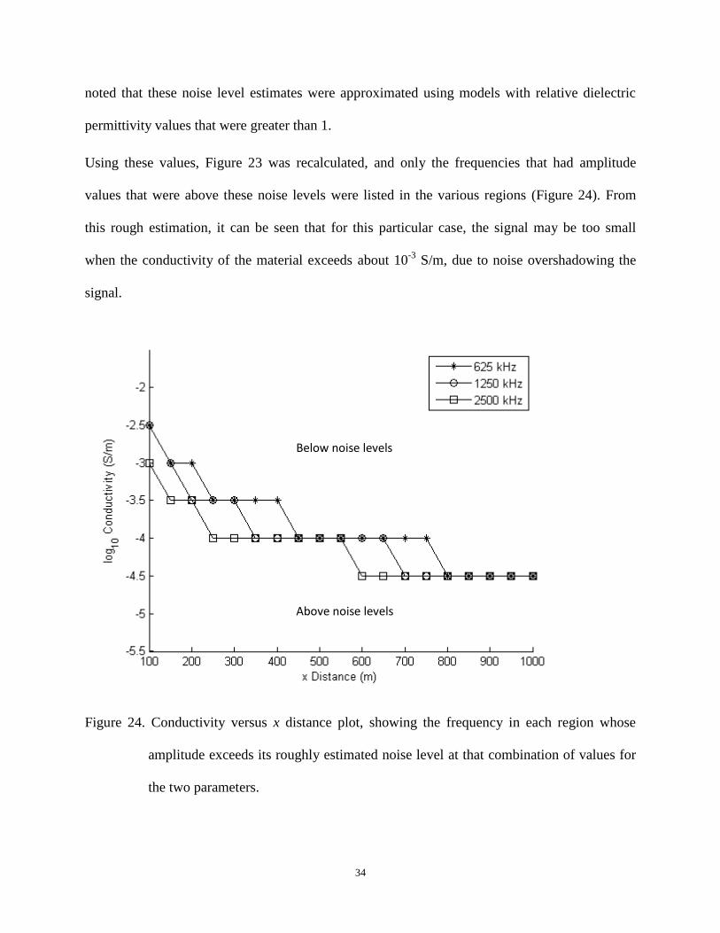
Using these values, Figure 23 was recalculated, and only the frequencies that had amplitude
values that were above these noise levels were listed in the various regions (Figure 24). From
this rough estimation, it can be seen that for this particular case, the signal may be too small
when the conductivity of the material exceeds about 10-3
S/m, due to noise overshadowing the
signal.
Figure 24. Conductivity versus x distance plot, showing the frequency in each region whose
amplitude exceeds its roughly estimated noise level at that combination of values for
the two parameters.
Below noise levels
Above noise levels

35
3.2.3 Angles
The effect of the angles of the boreholes was also investigated. As an example we looked at the
cases when the receiver hole is tilted 20 degrees towards the transmitter hole, and when the
transmitter hole is tilted 20 degrees towards the transmitter hole (Figure 25). The position of the
peak and the amplitude of the peak changes as the angles of the boreholes increase (Figure 26).
Figure 25. The two angled borehole geometries used for the simulations in Figure 26.
36
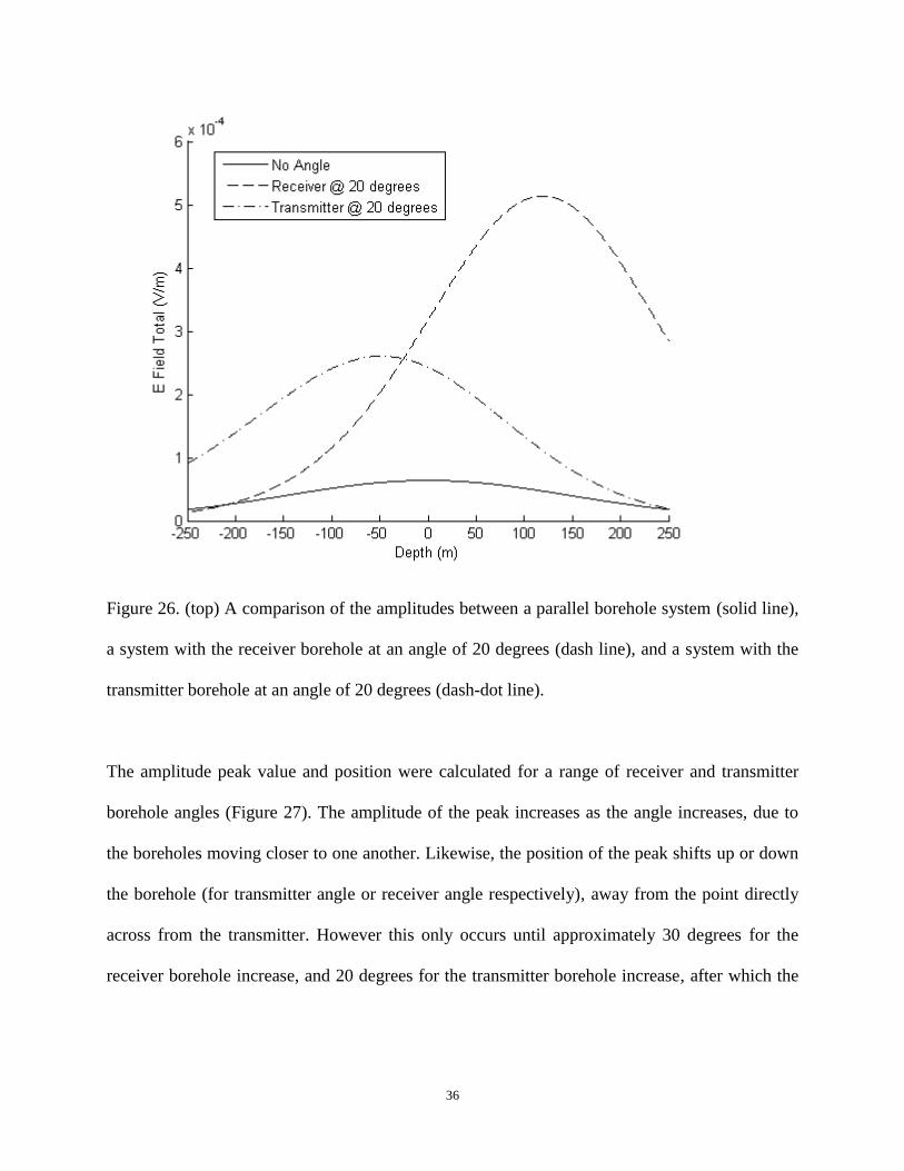
Figure 26. (top) A comparison of the amplitudes between a parallel borehole system (solid line),
a system with the receiver borehole at an angle of 20 degrees (dash line), and a system with the
transmitter borehole at an angle of 20 degrees (dash-dot line).
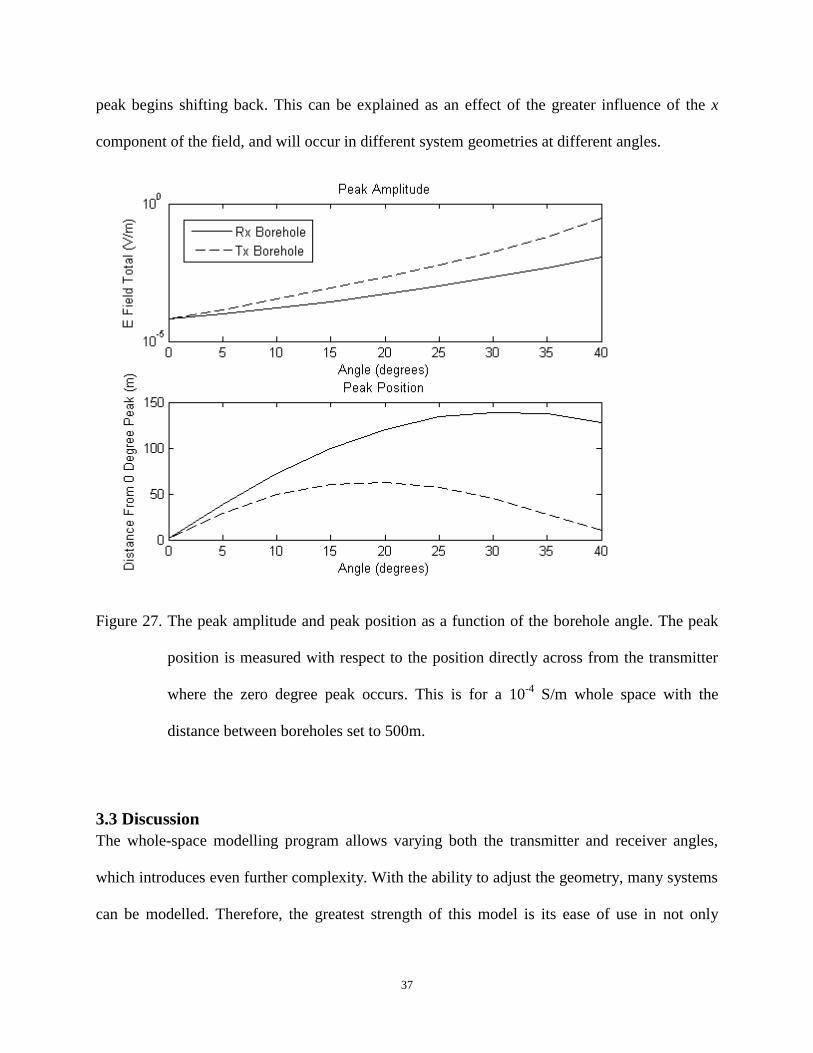
The amplitude peak value and position were calculated for a range of receiver and transmitter
borehole angles (Figure 27). The amplitude of the peak increases as the angle increases, due to
the boreholes moving closer to one another. Likewise, the position of the peak shifts up or down
the borehole (for transmitter angle or receiver angle respectively), away from the point directly
across from the transmitter. However this only occurs until approximately 30 degrees for the
receiver borehole increase, and 20 degrees for the transmitter borehole increase, after which the
37
peak begins shifting back. This can be explained as an effect of the greater influence of the x
component of the field, and will occur in different system geometries at different angles.
Figure 27. The peak amplitude and peak position as a function of the borehole angle. The peak
position is measured with respect to the position directly across from the transmitter
where the zero degree peak occurs. This is for a 10-4
S/m whole space with the
distance between boreholes set to 500m.
3.3 Discussion
The whole-space modelling program allows varying both the transmitter and receiver angles,
which introduces even further complexity. With the ability to adjust the geometry, many systems
can be modelled. Therefore, the greatest strength of this model is its ease of use in not only
38
investigating overarching patterns, but specific system configurations as well. The above
investigation of the patterns that occur from the parameters is not all-encompassing, but instead
has focused on several of the major parameters, and the general changes that occur with them.
This study has shown how specific parameters may affect data, however more can be
investigated and pursued if an understanding of a specific variation is required. For instance,
with more work, one possible area of investigation would be creating empirical equations to
some of these patterns. To do this, the modelling program could be used to generate a set of data
that could be correlated to create an analytic equation relating the peak position (and other
geometry) to the conductivity, such that, given a set of real data, an estimate for the conductivity
of the material could be found using only the geometric factors and the resulting data.
There are many of these possibilities with this whole-space modelling program, and as such, this
Parameter Investigation section should be seen primarily as an overview of the main parameters,
and the effects they have on the resulting signal. For more specific inquiries, the program itself
can be used.
4 Survey from Drury, Sudbury
To check the applicability of the whole-space model, we modelled field data from a survey in
Drury Township, near Sudbury, Ontario, Canada. The data were collected by GEOFARA using
the Fara RIM system on behalf of Sudbury Integrated Nickel Operations, a Glencore Company.
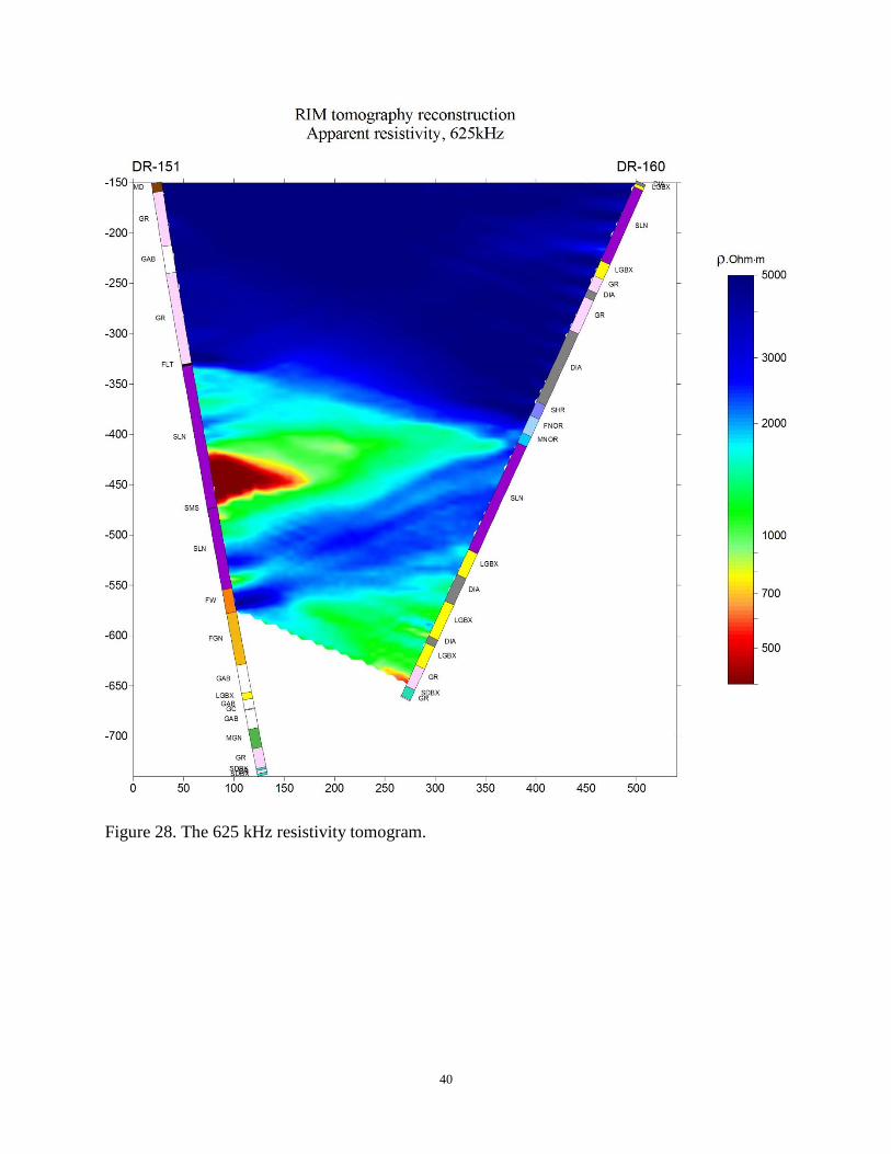
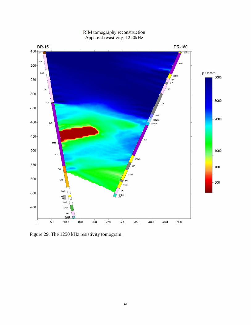
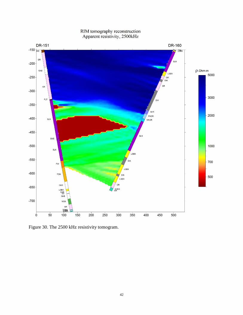
Figures 28, 29, and 30 show the conductivity tomograms created by GEOFARA. These plots
show the conductivity between boreholes DR-151 and DR-160 for transmitter frequencies of 625
39
kHz, 1250 kHz, and 2500 kHz respectively. Two data sets were collected at these three
frequencies: one set with the transmitter in DR-151 and the receiver in DR-160, and the
reciprocal set with the transmitter and receiver switched.
As can be seen, the area is divided by material of higher resistivity above approximately -325 m,
and material of lower resistivity below -325 m, with the greatest conductivity concentrated about
-450 m, closer to DR-151. There is a second conductive zone at -600 m closer to DR-160, with a
resistive zone separating these two zones. Comparing the three tomograms, it can be seen that
there is an overall trend of decreasing resistivity (increasing conductivity) as the frequency
increases. While it is most obvious in the very conductive zones (red and green), the resistive
zone above -325 m (blue) also tends towards a lower resistivity in the 1250 kHz and 2500 kHz
tomograms, as compared to the 625 kHz tomogram. Based on Figure 28, the area above -325 m
would range in conductivity anywhere from 2*10-4
S/m to 5*10-4
S/m, with the shallower depths
showing lower conductivity values. Below the -325 m depth there is a sharp increase in
conductivity.
40
Figure 28. The 625 kHz resistivity tomogram.
41
Figure 29. The 1250 kHz resistivity tomogram.
42
Figure 30. The 2500 kHz resistivity tomogram.
43
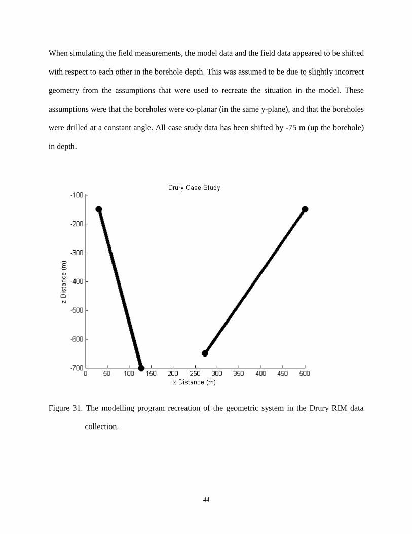
To recreate the data, the modelling program’s parameters were made to represent the field
situation as much as possible. The angles and distances were measured from the conductivity
tomograms (Figures 28-30). The system geometry that was input into the program is shown in
Figure 31.
The field data is organized by transmitter location. A location that was positioned in the resistive
upper zone was chosen, as the signal is less attenuated, resulting in clearer data. Additionally, the
upper resistive zone is fairly homogeneous, and therefore the modelling program should be able
to recreate the data effectively using the whole-space model. Accordingly, the data set with the
transmitter located at -275 m in borehole DR-160 was chosen for the case study.
Each transmitter location data set consists of amplitude and phase data for frequencies 625 kHz,
1250 kHz, and 2500 kHz. In recreating the data in the modelling program, each frequency data
set was fit separately from the other frequencies. The conductivity was adjusted until the phase
data peak position and sharpness matched that of the field data.
The phase data was used as the fitting method because the amplitude cannot be compared as
easily as the phase data. The field data amplitude is measured in an uncalibrated amplitude unit,
while the modelling program amplitude is measured in the physical units of the electric field
(V/m). The overall amplitude and trends can still be compared. However, for fitting the
conductivity, the phase data is much more effective.
The phase data collected by GEOFARA is exactly reversed in sign from the modelling program
phase data. As such, for this case study, the modelling program phase has been multiplied by a
factor of -1. Therefore all “rules of thumb” pertaining to phase described in the Parameter
Investigation section must be inverted for explanations here.
44
When simulating the field measurements, the model data and the field data appeared to be shifted
with respect to each other in the borehole depth. This was assumed to be due to slightly incorrect
geometry from the assumptions that were used to recreate the situation in the model. These
assumptions were that the boreholes were co-planar (in the same y-plane), and that the boreholes
were drilled at a constant angle. All case study data has been shifted by -75 m (up the borehole)
in depth.
Figure 31. The modelling program recreation of the geometric system in the Drury RIM data
collection.
45
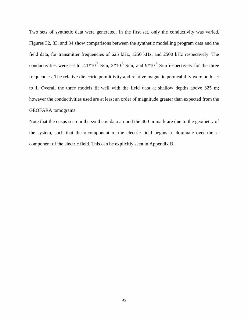
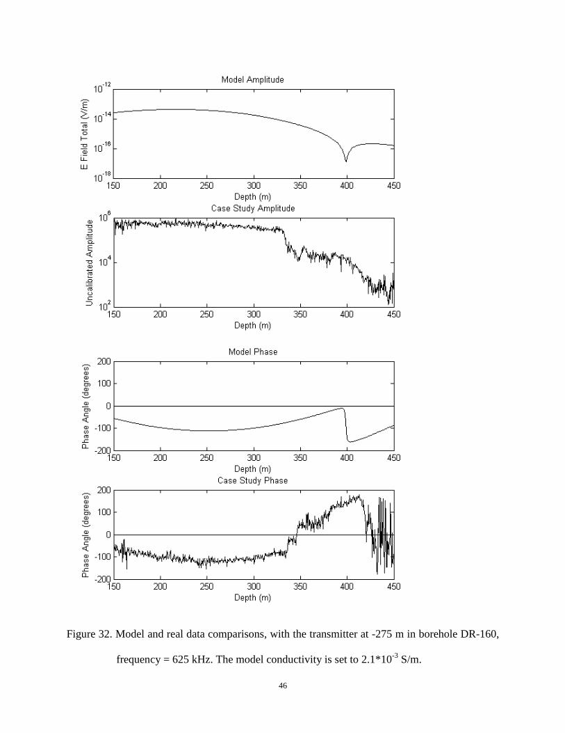
Two sets of synthetic data were generated. In the first set, only the conductivity was varied.
Figures 32, 33, and 34 show comparisons between the synthetic modelling program data and the
field data, for transmitter frequencies of 625 kHz, 1250 kHz, and 2500 kHz respectively. The
conductivities were set to 2.1*10-3
S/m, 3*10-3
S/m, and 9*10-3
S/m respectively for the three
frequencies. The relative dielectric permittivity and relative magnetic permeability were both set
to 1. Overall the three models fit well with the field data at shallow depths above 325 m;
however the conductivities used are at least an order of magnitude greater than expected from the
GEOFARA tomograms.
Note that the cusps seen in the synthetic data around the 400 m mark are due to the geometry of
the system, such that the x-component of the electric field begins to dominate over the z-
component of the electric field. This can be explicitly seen in Appendix B.
46
Figure 32. Model and real data comparisons, with the transmitter at -275 m in borehole DR-160,
frequency = 625 kHz. The model conductivity is set to 2.1*10-3
S/m.
47
Figure 33. Model and real data comparisons, with the transmitter at -275 m in borehole DR-160,
frequency = 1250 kHz. The model conductivity is set to 3*10-3
S/m.
48
Figure 34. Model and real data comparisons, with the transmitter at -275 m in borehole DR-160,
frequency = 2500 kHz. The model conductivity is set to 9*10-3
S/m.
49
In this set, two primary discrepancies can be seen.
The first discrepancy is simple to explain. Below the -325 m depth there is a sharp decrease in
amplitude and a sharp increase in phase. Based on the information obtained in the Parameter
Investigation section, this could be explained by a sudden increase in conductivity. This is
consistent with the conductive zone evident on the GEOFARA tomograms.
The other discrepancy is somewhat more subtle. In Figures 32 and 33 (625 kHz and 1250 kHz)
when the receiver in DR-151 is above the -250 m depth, as the depth decreases the field data
amplitude falls off at a slower rate than the synthetic data, and its associated phase data increases
towards 0 at a slower rate than the synthetic data. Both of these can be explained by a decrease in
conductivity as also evident in the Parameter Investigation section. The tomograms in Figures 28
and 29 (625 kHz and 1250 kHz) show that there is a small increase in resistivity above -250 m
near DR-151, and this is consistent with the observed behaviour in the measurements.
Above the -250 m depth, Figure 34 (2500 kHz) appears to show both a slight increase in
measured amplitude, as well as a slight increase in the rate of change of measured phase. This is
unlike the previous two cases, where the amplitude increased, but the phase rate of change was
slowed. The GEOFARA tomogram (Figure 30) shows an increase in resistivity, similar to the
other tomograms. So while the 2500 kHz synthetic data (Figure 34) still fits fairly well, there is
another possible explanation: the amplitude and phase variation might be indicative of a possible
increase in dielectric permittivity. As seen in the Parameter Investigation section, an increase in
amplitude, a reduction in the phase amplitude (or for the field data, an increase), and a
sharpening of the phase peak can be explained by an increase in dielectric permittivity. As
explained in Appendix C, the dielectric permittivity affects higher frequencies more drastically
than lower frequencies, and therefore by increasing the relative dielectric permittivity, this
50
discrepancy may be explained. Additionally, increasing the dielectric permittivity will increase
the amplitude values in all three frequency cases.
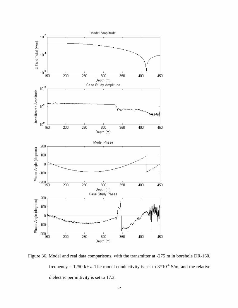
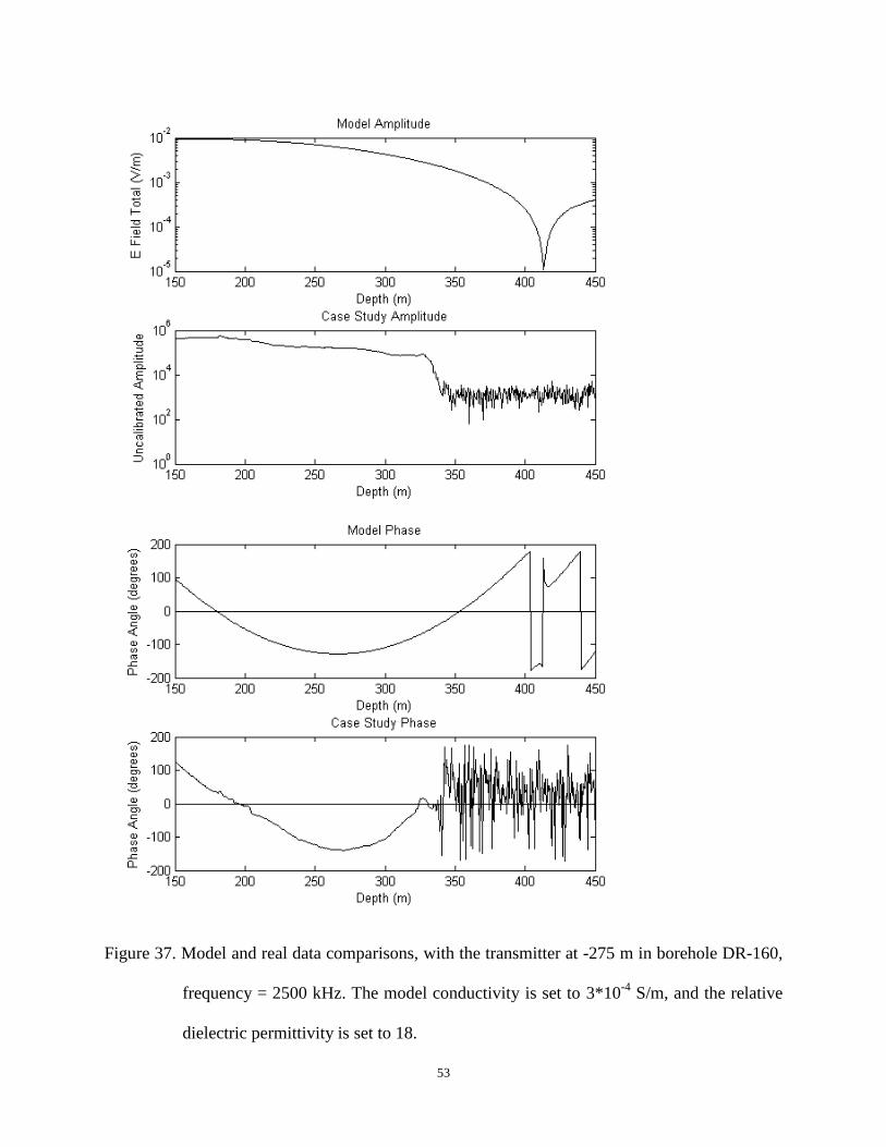
As such, another set of synthetic data were generated, setting the conductivity in the range
expected from the tomograms (approximately 3*10-4
S/m), followed by increasing the dielectric
permittivity. Figures 35 to 37 show these new data plots. The relative dielectric permittivity
values were set to 19.5, 17.3, and 18 for 625 kHz, 1250 kHz, and 2500 kHz respectively. It can
be seen that the synthetic amplitude plots are closer to the measured data, primarily above the -
225 m point, as compared to the previous set of data. The phase data still fits well and has not
changed significantly from the previous data.
51
Figure 35. Model and real data comparisons, with the transmitter at -275 m in borehole DR-160,
frequency = 625 kHz. The model conductivity is set to 3*10-4
S/m, and the relative
dielectric permittivity is set to 19.5.
52
Figure 36. Model and real data comparisons, with the transmitter at -275 m in borehole DR-160,
frequency = 1250 kHz. The model conductivity is set to 3*10-4
S/m, and the relative
dielectric permittivity is set to 17.3.
53
Figure 37. Model and real data comparisons, with the transmitter at -275 m in borehole DR-160,
frequency = 2500 kHz. The model conductivity is set to 3*10-4
S/m, and the relative
dielectric permittivity is set to 18.
54
From this case study, it can be concluded that the whole-space model may be used to simulate
real data effectively. Despite it being a homogeneous model, it can recreate sections of field data,
and the discrepancies between the model and the field data can be explained by inhomogeneity
in the physical properties, where the profiles diverge from those that are expected.
The difference between the case of synthetic data where only the conductivity was varied, and
the other case where conductivity was set to the expected value and dielectric permittivity was
varied, illustrates that the RIM method is sensitive to permittivity and that RIM modelling
programs should take permittivity into account.
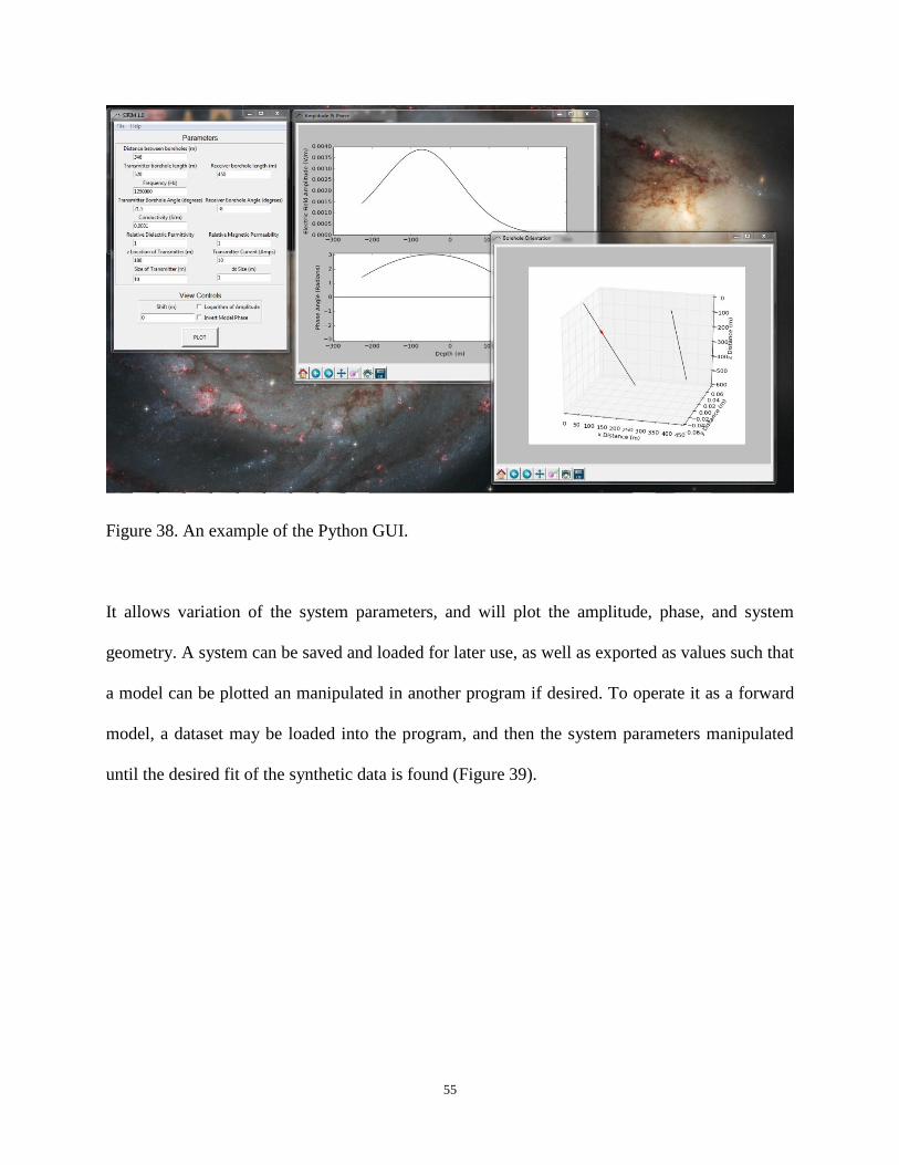
5 Forward Modelling Program
A GUI was built in Matlab for the modelling program, primarily for ease of use while
conducting both the Parameter Investigation as well as the Case Study. After realizing its
potential uses in quality assurance/quality control (QA/QC) as a forward model, the program was
ported to the Python language, such that it could be run without the need of the Matlab software.
As such, this program (Figure 38) is to be considered as a deliverable from this M.Sc. thesis.
55
Figure 38. An example of the Python GUI.
It allows variation of the system parameters, and will plot the amplitude, phase, and system
geometry. A system can be saved and loaded for later use, as well as exported as values such that
a model can be plotted an manipulated in another program if desired. To operate it as a forward
model, a dataset may be loaded into the program, and then the system parameters manipulated
until the desired fit of the synthetic data is found (Figure 39).
56
Figure 39. An example of the forward model capability of SIRIM. The black line is the synthetic
data, and the red line is the imported field data.
6 Conclusions
The formula for the electric field of a dipole in a whole space can be used to simulate the
response as measured by the radio imaging method. By varying a set of input parameters, a
better understanding of how the RIM amplitude and phase signal change has been obtained.
57
The use of the transmitter as an infinitesimal dipole is appropriate for calculations in almost all
situations. However in particularly conductive environments or configurations with small
borehole offsets, modelling the transmitter as two half-sized dipoles will remove most of the
error that could arise from incorrectly specifying the transmitter geometry.
A parameter investigation varied the input parameters (borehole offset, conductivity, dielectric
permittivity, and magnetic permeability) and key changes in the response were observed,
resulting in a set of “rules of thumb” as to how the amplitude and phase of the RIM signal is
expected to vary. These rules state that, in general, when increasing any of these four parameters,
predictable patterns in the value and shape of the amplitude and phase data can be expected.
Increasing the borehole separation causes both amplitude and phase peaks to broaden, decreases
the amplitude value, and shifts and the phase value negatively. Increasing the conductivity
causes similar changes, except the amplitude and phase peaks sharpen. Increasing the dielectric
permittivity causes the amplitude peak to broaden slightly, the phase peak to sharpen, and
increases amplitude values, but shifts phase values negatively. Increasing the magnetic
permeability causes the amplitude and phase peaks to sharpen, decreases the amplitude value,
and shifts the phase value negatively.
The effectiveness of different frequencies in various systems was investigated. As would be
expected, it was found that at smaller distances and in more resistive material, higher frequencies
would result in the highest amplitude, while at larger distances and more conductive systems,
lower frequencies result in significantly greater amplitudes. The magnitude to which these
generalities occurred was quantified: at distances greater than 300 metres and conductivities
58
greater than 10-4
S/m, lower frequencies dominated in effectiveness, as higher frequencies have
small amplitudes at these greater distances and conductivities.
Finally, an investigation of the effect of borehole angles showed that angles have a complex
effect on the signal, both “shifting” the data as well as increasing or decreasing the amplitude
value. These geometric effects should be taken into account in modelling so that their effects are
not misattributed to other factors such as the physical properties of the material.
The modelling program created was shown to be an effective forward model for RIM data. Using
data taken in Drury Township, near Sudbury, Ontario, Canada, field data from the more resistive
part of the hole was simulated in the modelling program with success. When forward modelling
field data, the whole-space model is effective at simulating measured data where both the
transmitter and receiver are in material that is uniformly conductive. The differences between the
model data and the field data can be explained and understood as variability in the conductivity,
and possibly the dielectric permittivity. The model was adjusted with the knowledge gained
from the parameter investigation. It was found that fitting with the phase data, and not the
amplitude, was much more effective when finding the appropriate conductivity value.
The whole-space modelling program can be effective as an investigative tool to better understand
how the RIM signal changes due to varying parameters, and for the forward modelling of real
data. As such a user-friendly version of the program was developed in Python for easy use and
distribution.

59
The ambiguity between conductivity and magnetic permeability may require further
investigation to gain a solid understanding of differing responses to changes in these two system
parameters. Additionally, further analysis of the effect of angles on the response may prove to be
beneficial. As such, it is recommended that these two issues be further studied.
It is finally recommended that the modelling program be further developed to include a y-axis
offset, as this may help account for errors due to geometry, such as the -75 m shift required in the
case study.
60
7 References
Fullagar, P., D. Livelybrooks, P. Zhang, A. Clavert, and Y. Wu, 2000, Radio tomography and
borehole radar delineation of the McConnell nickel sulfide deposit, Sudbury, Ontario, Canada
Geophysics, 65, 1920–1930.
Holliger, K., Musil, M., Maurer, H.R., 2001, Ray-based amplitude tomography for crosshole
georadar data: a numerical assessment, Journal of Applied Geophysics, 47, 285–298.
Jang, H., M. Park, and H. Kim, 2006, Numerical modeling of antenna transmission for borehole
ground-penetrating radar, Proceedings of the 8th SEGJ International Symposium, 1-6.
Johnson, D., 1997, Finite Difference Time Domain Modelling of Cross-Hole Electromagnetic
Survey Data: M.S. thesis, University of Utah.
Karimi Sharif, L., 2013, Application of the cross-hole Radio Imaging Method in detecting
geological anomalies, MacLennan Township, Sudbury Ontario: M.S. thesis, Laurentian
University.
Korpisalo A., Heikkinen E., 2014, Radiowave imaging research (RIM) for determining the
electrical conductivity of the rock in borehole section OL-KR4-OL-KR10 at Olkiluoto, Finland,
Exploration Geophysics, http://dx/doi.org/10.1071/EG13057.
61
Livelybrooks, D., Chouteau, M., Zhang, P., Stevens, K., and Fullagar, P., 1996, Borehole radar
and radio imaging surveys to delineate the McConnell ore body near Sudbury, Ontario, SEG
Technical Program Expanded Abstracts, 2060-2063.
Mutton, A.J., 2000. The application of geophysics during evaluation of the Century zinc deposit,
Geophysics, vol. 65, no. 6, 1946-60.
Pears G.A., P.K. Fullagar, 1998, Weighted tomographic imaging of radio frequency data,
Exploration Geophysics, 29, 554–559.
Stevens, K., Watts, A. and Redko, G., 2000. In-Mine Applications of the Radio-Wave Method in
the Sudbury Igneous Complex. Paper presented at the 2000 SEG Annual Meeting.
Stolarczack, L. G., Fry, R. C., 1986, Radio imaging method (RIM) or diagnostic imaging of
anomalous geologic structures in coal seam waveguides. Transactions of the Society for
Mining, Metallurgy, and Exploration, Inc., 288, 1806-1814.
Thomson, S., J. Young, and N. Sheard, 1992, Base metal applications of the radio imaging
method. Current status and case studies, Exploration Geophysics, 23, 367–372.
Ward, S. H., and G. W. Hohmann, 1987, Electromagnetic theory for geophysical applications, in
M. N. Nabighian, ed., Electromagnetic methods in applied geophysics I: SEG, 131-312.
62
Zhou B., Fullagar P. K., Delineation of sulphide ore-zones by borehole radar tomography at
Hellyer Mine, Australia, Journal of Applied Geophysics, 47, July 2001, 261-269.
Zhou, B., Fullagar, P.K. and Fallon, G.N., 1998. Radio frequency tomography trial at Mt Isa
Mine. Exploration Geophysics, vol. 29, no. 3-4, 675-679.
63
Appendix A: Noise Level
To get the noise level approximations used in section 3.2.2 Frequency Variation, the following
process and calculations were completed.
Noise may vary from survey to survey, however an approximation can be found by comparing
real data with synthetic data. To do this, data from the Drury County survey (used in the Case
Study section) was analyzed to find noise levels for each of the three frequencies used in the
survey.
The Fara RIM amplitude is measured in a form of uncalibrated amplitude values and not in the
electric field units V/m. To convert the uncalibrated values to V/m, the field measurements were
simulated in the modelling program as in the Case Study section, and several values were
compared between the two data sets (Figure 40). It is important to note that the simulations used
varied values of the dielectric permittivity, and could affect the precision of the results in this
analysis.
64
Figure 40. Example of the comparison of the synthetic data amplitude and the field data
amplitude with the transmitter at -275 m in borehole DR-160, frequency = 1250 kHz.
The model conductivity is set to 3*10-4
S/m, and the relative dielectric permittivity is
set to 17.3. The arrows show the points of comparison used.
To convert the field data to units of V/m, a direct linear comparison is used:
Field Data = A * Synthetic Data (14)
Where A is a constant to be determined.
65
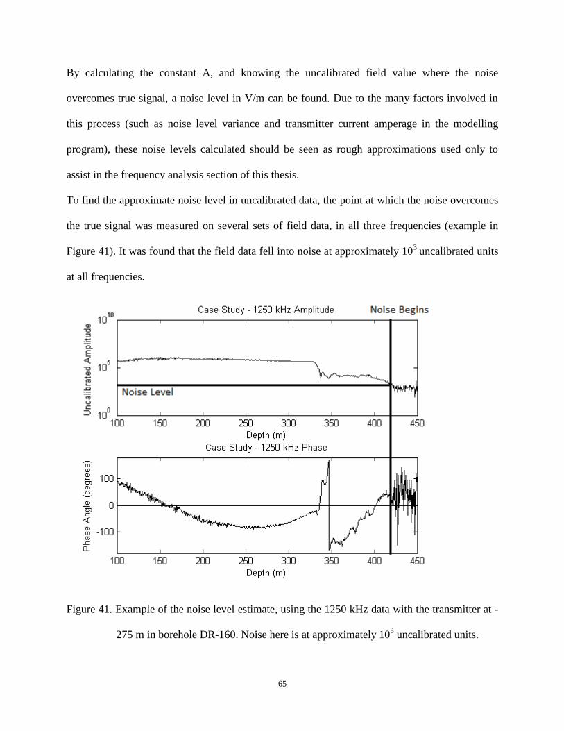
By calculating the constant A, and knowing the uncalibrated field value where the noise
overcomes true signal, a noise level in V/m can be found. Due to the many factors involved in
this process (such as noise level variance and transmitter current amperage in the modelling
program), these noise levels calculated should be seen as rough approximations used only to
assist in the frequency analysis section of this thesis.
To find the approximate noise level in uncalibrated data, the point at which the noise overcomes
the true signal was measured on several sets of field data, in all three frequencies (example in
Figure 41). It was found that the field data fell into noise at approximately 103
uncalibrated units
at all frequencies.
Figure 41. Example of the noise level estimate, using the 1250 kHz data with the transmitter at -
275 m in borehole DR-160. Noise here is at approximately 103 uncalibrated units.
66
Below are noise level calculations for each of the three frequencies used in the field data set (625
kHz, 1250 kHz, and 2500 kHz). 312.5 kHz was not used in the field data set, and as such, is not
used here.
625 kHz
Synthetic Data – 0.0008911 V/m
Field Data – 5.465*105 field units
Therefore A = 6.133*108 field units/V/m
Using the noise level as 103 field units equals approximately 1.6*10
-6 V/m.
1250 kHz
Synthetic Data – 0.002031 V/m
Field Data – 8.004*105 field units
Therefore A = 3.941*108 field units/V/m
Using the noise level as 103 field units equals approximately 2.5*10
-6 V/m.
2500 kHz
Synthetic Data – 0.008878 V/m
Field Data – 3.912*105 field units
Therefore A = 4.406*107 field units /V/m
Using the noise level as 103 field units equals approximately 2.3*10
-5 V/m.
67
Appendix B: Case Study Synthetic Data Cusps
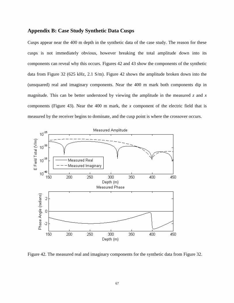
Cusps appear near the 400 m depth in the synthetic data of the case study. The reason for these
cusps is not immediately obvious, however breaking the total amplitude down into its
components can reveal why this occurs. Figures 42 and 43 show the components of the synthetic
data from Figure 32 (625 kHz, 2.1 S/m). Figure 42 shows the amplitude broken down into the
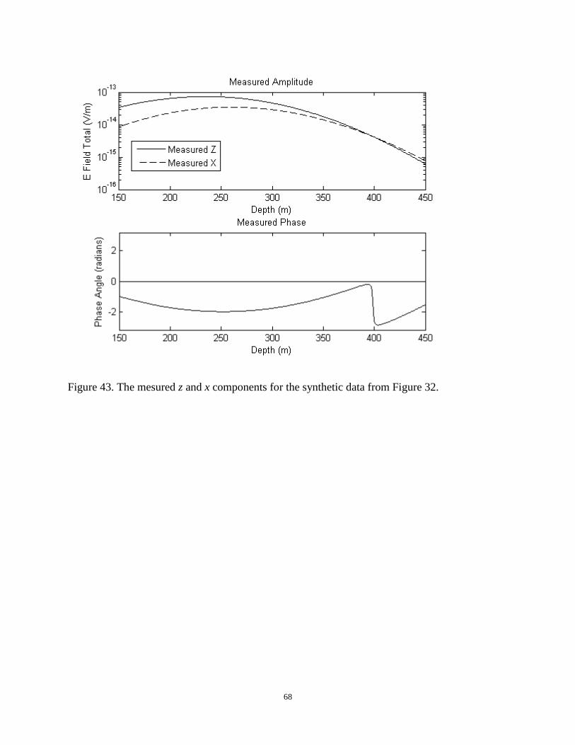
(unsquared) real and imaginary components. Near the 400 m mark both components dip in
magnitude. This can be better understood by viewing the amplitude in the measured z and x
components (Figure 43). Near the 400 m mark, the x component of the electric field that is
measured by the receiver begins to dominate, and the cusp point is where the crossover occurs.
Figure 42. The measured real and imaginary components for the synthetic data from Figure 32.
68
Figure 43. The mesured z and x components for the synthetic data from Figure 32.
69
Appendix C: Frequency and Dielectric Permittivity
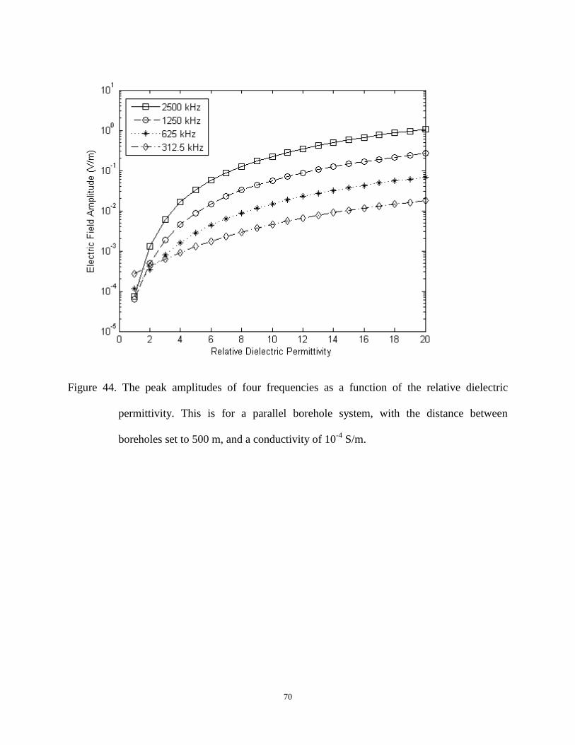
Similar to the distance and conductivity range plots (Figures 20 and 21), a plot of the peak
amplitudes over a range of dielectric permittivity values was built with the whole-space
modelling program (Figure 44). From this, it can be seen that increasing values of the dielectric
permittivity increases the amplitude in all cases; however the affects at higher frequencies are
more drastic than the lower frequencies. This is also the case for the corresponding phase part of
the signal.
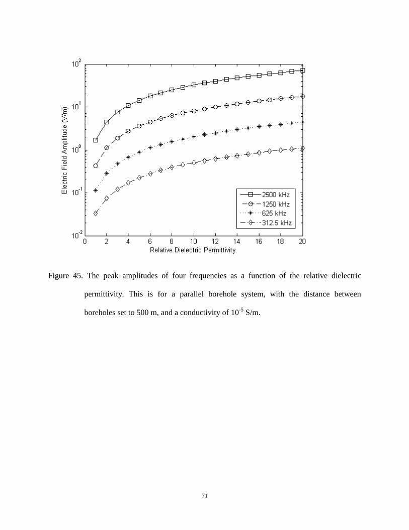
Increasing or decreasing the conductivity and re-calculating this data shows the same trend of
higher frequencies being affected more, combined with the effect of the conductivity change
(Figures 45 and 46). As expected, a lower conductivity results in the amplitude of the higher
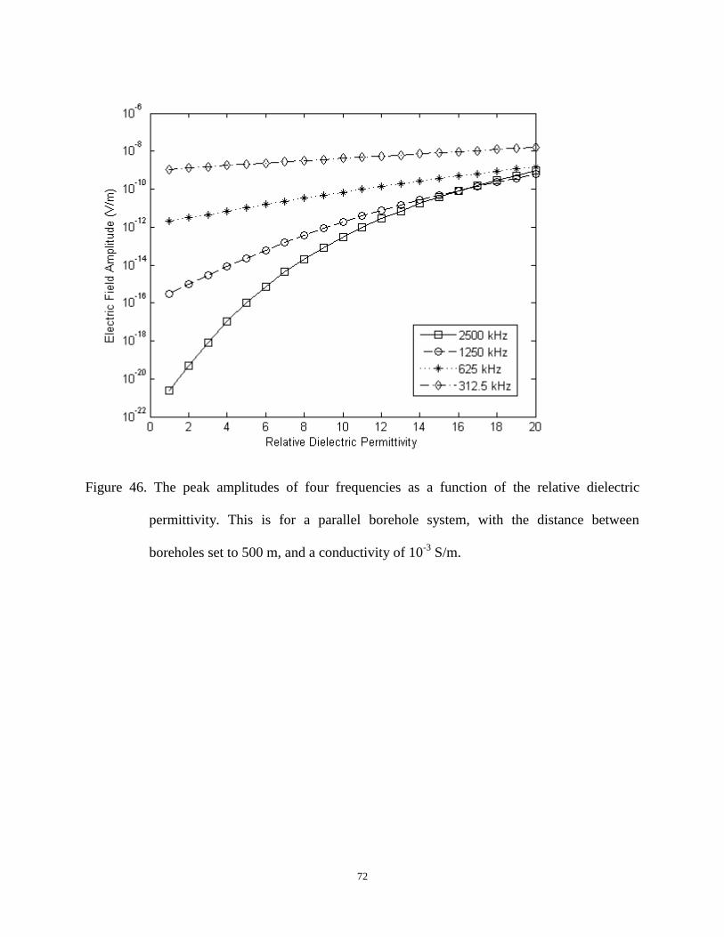
frequencies being greater than the amplitude of the lower frequencies (Figure 45). A greater
conductivity results in the amplitude of the lower frequencies being greater than the amplitude of
the higher frequencies; however, as the relative dielectric permittivity increases, the higher
frequencies’ amplitudes increase at a much greater rate than the amplitudes of the lower
frequencies (Figure 46).
70
Figure 44. The peak amplitudes of four frequencies as a function of the relative dielectric
permittivity. This is for a parallel borehole system, with the distance between
boreholes set to 500 m, and a conductivity of 10-4
S/m.
71
Figure 45. The peak amplitudes of four frequencies as a function of the relative dielectric
permittivity. This is for a parallel borehole system, with the distance between
boreholes set to 500 m, and a conductivity of 10-5
S/m.
72
Figure 46. The peak amplitudes of four frequencies as a function of the relative dielectric
permittivity. This is for a parallel borehole system, with the distance between
boreholes set to 500 m, and a conductivity of 10-3
S/m.