Embed Size (px)
Citation preview
University of Wollongong University of Wollongong
Research Online Research Online
University of Wollongong Thesis Collection 1954-2016 University of Wollongong Thesis Collections
2015
Modelling of inverter interfaced renewable energy resources to investigate Modelling of inverter interfaced renewable energy resources to investigate
grid interactions grid interactions
Brian K. Perera University of Wollongong, [email protected]
Follow this and additional works at: https://ro.uow.edu.au/theses
University of Wollongong University of Wollongong
Copyright Warning Copyright Warning
You may print or download ONE copy of this document for the purpose of your own research or study. The University
does not authorise you to copy, communicate or otherwise make available electronically to any other person any
copyright material contained on this site.
You are reminded of the following: This work is copyright. Apart from any use permitted under the Copyright Act
1968, no part of this work may be reproduced by any process, nor may any other exclusive right be exercised,
without the permission of the author. Copyright owners are entitled to take legal action against persons who infringe
their copyright. A reproduction of material that is protected by copyright may be a copyright infringement. A court
may impose penalties and award damages in relation to offences and infringements relating to copyright material.
Higher penalties may apply, and higher damages may be awarded, for offences and infringements involving the
conversion of material into digital or electronic form.
Unless otherwise indicated, the views expressed in this thesis are those of the author and do not necessarily Unless otherwise indicated, the views expressed in this thesis are those of the author and do not necessarily
represent the views of the University of Wollongong. represent the views of the University of Wollongong.
Recommended Citation Recommended Citation Perera, Brian K., Modelling of inverter interfaced renewable energy resources to investigate grid interactions, Doctor of Philosophy thesis, School of Electrical, Computer and Telecommunications Engineering, University of Wollongong, 2015. https://ro.uow.edu.au/theses/4561
Research Online is the open access institutional repository for the University of Wollongong. For further information contact the UOW Library: [email protected]

School of Electrical, Computer and Telecommunications Engineering
Modelling of Inverter Interfaced Renewable
Energy Resources to Investigate Grid
Interactions
Brian Perera, BSc (Eng)
Supervisors
Dr Philip Ciufo and Professor Sarath Perera
This thesis is presented as part of the requirements for the
Award of the Degree of
Doctor of Philosophy
of the
University of Wollongong
March 2015

2

Dedicated to my parents and my family...

ii

Acknowledgements
I wish to express my sincere appreciation to all the people who helped me in
many ways throughout my PhD candidature at the University of Wollongong.
I would like to pay my greatest gratitude and appreciation to my principal
supervisor, Dr Phil Ciufo and my co-supervisor, Professor Sarath Perera of the
University of Wollongong (UOW), for providing me the opportunity to pursue
postgraduate studies at UOW. My supervisors’ dedication, patience, knowledge
and experience could not have been surpassed. I admire their guidance towards
growing me up academically and personally over last few years.
My PhD research project was funded by the Australian Research Council
(ARC) and Essential Energy through the Linkage Grant LP100100618. Without
the financial support received from these organisations, my dream to complete
a PhD degree may not have been realised. The guidance of Chief Investigators
of this research project, Associate Professor Kashem Muttaqi, Professor Danny
Sutanto and my supervisors and the Partner Investigator, Leith Elder, Senior
Engineer, Essential Energy to reach the goals of the project is also highly appre-
ciated.
The personal and administrative support provided by Sasha Nikolic, Roslyn
Causer-Temby, Raina Lewis, Megan Crowl and Esperanza Gonzalez at various
stages of my PhD degree are acknowledged with gratitude. Special thanks go to
Dr Vic Smith, Dr Sridhar Pulikanti, Sean Elphick, Hamid Ghasemabadi and Dr
Douglas Carter for their generous technical support provided while establishing
the laboratory experimental setup of my research project. Timely technical assis-
tances received from Carlo Giusti, Frank Mikk, Steve Petrou and Neil Wood were
key factors of being able to commission the experimental setup of my research
project within a short period of time. I am very much thankful to them.
I would like to thank Dr Nishad Mendis and Dr Upuli Jayatunga for the
support given during my candidature. Thanks also go to my fellow graduate stu-
dents Devinda Perera, Amila Wickramasinghe, Dothinka Ranamuka and Athmi
iii

Jayawardena for their valuable input to my research work.
Last but not least, I would like to thank my parents, Damian Perera and
Marie Fernando, my wife, Aishanee Weerasundara and the rest of my family for
their unconditional love and continuous support. I would not have been able to
complete this Thesis without them.
iv

Certification
I, Brian Perera, declare that this thesis, submitted in fulfilment of the require-
ments for the award of Doctor of Philosophy, in the School of Electrical, Computer
and Telecommunications Engineering, University of Wollongong, is entirely my
own work unless otherwise referenced or acknowledged. This manuscript has not
been submitted for qualifications at any other academic institute.
Brian Perera
v

vi

Abstract
The public low voltage (LV) electricity networks are being increasingly impacted
by the connection of many small-capacity solar photovoltaic (PV) systems. These
PV systems offer financial benefits to owners while bringing environmental ben-
efits by reducing the electricity generation using fossil fuels. However, there are
technical challenges that should be addressed in order to enable the smooth in-
tegration of PV systems to public LV electricity networks.
A detailed simulation model of a PV system is a useful tool for analysing the
system-level impact of integrating multiple PV systems to public LV electricity
networks. Therefore, such a simulation model of a grid-connected single-phase
two-stage PV system with associated controllers is developed in this Thesis. The
accuracy of the developed simulation model is validated by comparing simulation
results with experimental results obtained from a comparable experimental PV
system established in the laboratory. The developed simulation model of a PV
system forms the basis for the rest of the work presented in this Thesis.
The introduction of multiple PV systems may result in public LV electricity
networks becoming more susceptible to voltage variations and fluctuations caused
by the injected active power variations from the PV systems. Furthermore, if the
power generation by PV systems exceeds that of the local load demand, there is a
possibility of power flowing into the grid for which the traditional LV systems are
not designed. As a result, there can be over voltages in the LV network leading
to tripping of PV systems. The voltage rise in public LV electricity networks
integrated with multiple PV systems is a critical technical problem that should
be addressed. Traditional voltage control techniques are not adequate under
such situations. As a consequence, there is a demand for fast acting dynamic
voltage regulating devices which can respond within a short period of time to the
variations and restore the system to its normal operation.
An opportunity exists to regulate the respective point of common coupling
(PCC) voltages by dynamically controlling both active and reactive power injec-
vii
tion by PV systems that are integrated to an public LV electricity network via
voltage source converters. In this Thesis, two closed-loop controllers that are able
to regulate the PCC voltage by dynamically controlling the active and reactive
power of a PV system are developed. The dynamic behaviour of each controller
is analysed in detail. By combining the dynamic active and reactive power con-
trollers, two novel operating strategies for PV systems; fixed minimum power
factor operation and fixed maximum apparent power operation, are proposed.
The simulation results are validated using experimental work confirming the ac-
curacy of the derived plant models, the robustness of the designed controllers
and the feasibility of implementing the proposed novel operating strategies in PV
systems.
In a public LV electricity network, to which multiple PV systems are in-
tegrated, the grid voltage can be controlled if each PV system regulates their
respective PCC voltage. In such an application of PV systems, the possibility of
control interactions between PV systems exists since PV systems operate elec-
trically close to each other. In this Thesis, possible control interactions between
multiple PV systems are investigated and results of simulation studies are pre-
sented. The small-signal model of an LV radial power distribution feeder with
multiple PV systems developed in this Thesis is used to perform modal analysis to
verify identified control interactions. The experimental results presented confirm
that there are control interactions between multiple PV systems when these sys-
tems control the grid voltage dynamically by absorbing reactive power from the
grid. The control techniques that can be applied to minimise the effects of control
interaction between PV systems are discussed and validated experimentally.
According to applicable standards for grid-integrated PV systems, a PV sys-
tem must be disconnected from the grid when the terminal voltage of the PV
system exceeds a defined maximum voltage. With this directive, in certain situ-
ations, PV systems connected at nodes at which the voltage sensitivity is high,
may get disconnected from the grid while PV systems connected at less sensitive
viii

nodes continue to operate. In such a situation, owners whose PV systems are con-
nected at nodes at which the voltage sensitivity is high, may lose their revenue.
In order to minimise the impact of such a disadvantage, a power sharing method-
ology that can be implemented in PV systems connected to a radial distribution
feeder is developed in this Thesis. In the developed method, power sharing is
achieved by operating PV systems within an allocated voltage bandwidth that
is applicable to the PCC voltage of a PV system. The developed power sharing
methodology provides a pathway to share power injection by PV systems instead
of leading to the disconnection of some PV systems and not others, which leads
to an inequitable operating environment.
The analytical tools and experimentally validated simulation models that are
developed in this Thesis will be beneficial for electricity distribution utilities who
at present, have to deal with uncertainties related to the impact of high pene-
tration levels of PV systems in their LV electricity networks. Further, advanced
control and coordination techniques and methodologies developed in this Thesis
will also enable the development of proper coordination and control strategies
which should be adopted for voltage control and reactive power compensation
while improving system stability and efficiency.
ix

x
List of principal symbols and abbreviations
A/D analog to digital
AC alternating current
BWx bandwidth
Cb base capacitance
Cdc DC-link capacitor of a VSC
Cf capacitor of an LCL filter
Cpv filtering capacitor at the output of a PV array
CSC current source converter
D duty ratio
D/A digital to analog
DC direct current
δ power angle
∆Ix small change in current
∆Vdc magnitude of the DC-link voltage ripple
∆Vx small change in voltage
DSP digital signal processor
DSTATCOM distribution static synchronous compensator
Enp PCC VP controller enable signal
Enq PCC VQ controller enable signal
fdc switching frequency of a DC-DC boost converter in Hz
fres resonant frequency in Hz
fsw switching frequency of a VSC in Hz
FACTS flexible AC transmission system
Hbp gain of a band-pass filter
HC harmonic compensator
i output current of a VSC
Idc current flow through the DC-link
Idpv current conducted by the diode of a PV cell model
ig current injected to the grid by a VSC
Ig rms value of ig
Igp active current component of Ig
Igmp peak value of Igp
xi

Igq reactive current component of Ig
Igmq peak value of Igq
Igmq0 initial value of Igmq
Igpmref current reference of Igpm
igref current reference of ig
Ipv current output of a PV array or PV cell
Ipvref current reference of Ipv
Igqmref current reference of Igqm
Iscpv saturation current of the diode of a PV cell model
IGBT insulated gate bi-polar transistor
InC incremental conductance
k Boltzmann’s constant (1.38× 10⁻²³ J/K)
kix integral gain
kpx proportional gain
L live conductor
Ldc inductor of a DC-DC boost converter
Lfc inductance of the converter-side inductor of an LCL filter
Lfg inductance of the grid-side inductor of an LCL filter
Lg inductance of Xg
LMS least-mean-square
LV low voltage
m modulation signal
MOSFET metaloxidesemiconductor field-effect transistor
MPP maximum power point
MPPT maximum power point tracking
N neutral conductor
nd diode quality factor (1¡n¡2)
Nx electrical node
nh harmonic number
ω fundamental frequency in rad/s
ωe estimated frequency of vg in rad/s
ωbp centre frequency of a band-pass filter in rad/s
ωc cut-off frequency in rad/s
P active power
xii

P & O perturb and observe
Pc active power output of a VSC
Pdc power flow through the DC-link
Pg active power injected to the grid by a PV system
Pmpp power available at MPP
Pn nominal active power
Ppv power output of a PV array
Pref active power reference of Pg
PCC point of common coupling
PI proportional-integral
PLL phase-locked-loop
PR proportional-resonant
PSS power system stabiliser
PV solar photovoltaic
q electron charge (1.602× 10⁻¹⁹ As)
Q reactive power
Qbp quality factor of a band-pass filter
Qc reactive power output of a VSC
Qg reactive power injected to the grid by a PV system
Qref reactive power reference of Qg
R/X resistance to reactance
Rd damping resistor in series with Cf
Rfc resistance of the converter-side inductor of an LCL filter
Rfg resistance of the grid-side inductor of an LCL filter
Rg resistive component of grid impedance
Rshpv shunt resistance of a PV cell
Rsrpv series resistance of a PV cell
rms root-mean-square
Sb base power
Sr kVA rating of a VSC
s-PLL synchronous reference frame PLL
SPWM sinusoidal pulse-width modulation
τd time constant of a first-order lag element
THD total harmonic distortion
xiii
ϑ estimated phase angle of vg
Umax 253 V
v output voltage of a VSC
Vα α-axis voltage
Vβ β-axis voltage
v0 fundamental voltage component of v
Vb base voltage
vc voltage across Cf and Rd
Vdc DC-link voltage of a VSC
Vdcavg average DC-link voltage
Vdcref DC-link voltage reference
Vdpv voltage across the diode of a PV cell model
vg voltage at the PCC of a VSC
Vg rms value of vg
Vgm peak value of vg
Vgm0 initial value of Vgm
Vgmref voltage reference of Vgm
Vmpp voltage at MPP
Vmpp0 initial Vmpp
Vocpv open circuit voltage of a PV array
Vpv voltage output of a PV array or a PV cell
Vpvref voltage reference of Vpv
vs voltage of the equivalent Thevenin voltage source
Vs rms value of vs
Vd d-axis voltage
Vgx rms voltage at node x
Vq q-axis voltage
VCO voltage-controlled-oscillator
VSC voltage source converter
Xg reactive component of grid impedance
xqx state variable
Yij admittance between node i and j
Zb base impedance
xiv

Publications Arising from the Thesis
1. Brian Perera, Phil Ciufo and Sarath Perera. Simulation Model of a Grid-
Connected Single-Phase Photovoltaic System in PSCAD/EMTDC. In Proc.
IEEE International Conference on Power System Technology (POWER-
CON), Auckland, New Zealand, October 2012.
2. Brian Perera, Phil Ciufo and Sarath Perera. Power Sharing among Multiple
Solar Photovoltaic (PV) Systems in a Radial Distribution Feeder. In Proc.
Australasian Universities Power Engineering Conference (AUPEC 2013),
Vienna, Austria, October 2013.
3. Brian Perera, Phil Ciufo and Sarath Perera. Point of Common Coupling
(PCC) Voltage Control of a Grid-Connected Solar Photovoltaic (PV) Sys-
tem. In Proc. 39th Annual Conference of the IEEE Industrial Electronics
Society (IECON’13), Vienna, Austria, November 2013.
4. Brian Perera, Phil Ciufo and Sarath Perera. Advanced Point of Common
Coupling Voltage Controllers for Grid-Connected Solar Photovoltaic (PV)
Systems. Accepted for publication in Elsevier - Renewable Energy Journal.
xv

xvi

Table of Contents
1 Introduction 11.1 Statement of the Problem . . . . . . . . . . . . . . . . . . . . . . 11.2 Research Objectives and Methodologies . . . . . . . . . . . . . . . 51.3 Outline of the Thesis . . . . . . . . . . . . . . . . . . . . . . . . . 8
2 Literature Review 112.1 Introduction . . . . . . . . . . . . . . . . . . . . . . . . . . . . . . 112.2 Solar photovoltaic energy . . . . . . . . . . . . . . . . . . . . . . . 12
2.2.1 Equivalent circuit of a PV cell . . . . . . . . . . . . . . . . 122.2.2 Terminal characteristics of a PV cell . . . . . . . . . . . . 132.2.3 Maximum power point tracking (MPPT) . . . . . . . . . . 14
2.3 Power converters for integrating PV systems to the grid . . . . . . 152.4 Operation and control of a VSC . . . . . . . . . . . . . . . . . . . 17
2.4.1 Basic operation of a VSC . . . . . . . . . . . . . . . . . . . 172.4.2 Four-quadrant operation of a VSC . . . . . . . . . . . . . 212.4.3 Control systems in a VSC . . . . . . . . . . . . . . . . . . 22
2.5 Grid-connected PV system . . . . . . . . . . . . . . . . . . . . . . 262.6 Impact of the integration of multiple PV systems on an LV power
grid . . . . . . . . . . . . . . . . . . . . . . . . . . . . . . . . . . 272.6.1 Steady-state voltage rise with connection of PV systems to
a power distribution feeder . . . . . . . . . . . . . . . . . . 292.6.2 Voltage level variations in an LV power grid integrated with
multiple PV systems . . . . . . . . . . . . . . . . . . . . . 312.7 Voltage control in an LV power grid integrated with multiple PV
systems . . . . . . . . . . . . . . . . . . . . . . . . . . . . . . . . 322.8 Application of distribution static synchronous compensator (DSTAT-
COM) . . . . . . . . . . . . . . . . . . . . . . . . . . . . . . . . . 352.9 Operational and control interactions between multiple PV systems 362.10 Control and coordination of the operation of multiple PV systems 372.11 Chapter summary . . . . . . . . . . . . . . . . . . . . . . . . . . . 39
3 Simulation model of a PV system 413.1 Introduction . . . . . . . . . . . . . . . . . . . . . . . . . . . . . . 413.2 Modelling . . . . . . . . . . . . . . . . . . . . . . . . . . . . . . . 43
3.2.1 PV array . . . . . . . . . . . . . . . . . . . . . . . . . . . 433.2.2 MPPT algorithm . . . . . . . . . . . . . . . . . . . . . . . 443.2.3 Voltage source converter . . . . . . . . . . . . . . . . . . . 463.2.4 LCL filter . . . . . . . . . . . . . . . . . . . . . . . . . . . 463.2.5 Selection of DC-link capacitor . . . . . . . . . . . . . . . . 463.2.6 DC-DC boost converter . . . . . . . . . . . . . . . . . . . 473.2.7 LV power grid . . . . . . . . . . . . . . . . . . . . . . . . . 48
3.3 Control system design . . . . . . . . . . . . . . . . . . . . . . . . 483.3.1 Grid synchronisation . . . . . . . . . . . . . . . . . . . . . 483.3.2 Current controller . . . . . . . . . . . . . . . . . . . . . . . 513.3.3 DC-link voltage controller . . . . . . . . . . . . . . . . . . 533.3.4 DC-DC boost converter controller . . . . . . . . . . . . . . 56
xvii

3.3.5 Power factor controller . . . . . . . . . . . . . . . . . . . . 573.4 Simulation results . . . . . . . . . . . . . . . . . . . . . . . . . . . 573.5 Experimental results . . . . . . . . . . . . . . . . . . . . . . . . . 613.6 Chapter summary . . . . . . . . . . . . . . . . . . . . . . . . . . . 71
4 PCC voltage control of a grid-connected PV system 754.1 Introduction . . . . . . . . . . . . . . . . . . . . . . . . . . . . . . 754.2 Simplified model of a distribution feeder . . . . . . . . . . . . . . 764.3 Decoupling of controllers . . . . . . . . . . . . . . . . . . . . . . . 774.4 PCC voltage regulation with the dynamic reactive power controller
- (PCC VQ controller) . . . . . . . . . . . . . . . . . . . . . . . . . 784.4.1 Control plant model of the PCC VQ controller . . . . . . . 784.4.2 PCC VQ controller . . . . . . . . . . . . . . . . . . . . . . 804.4.3 PCC VQ controller - with a proportional gain . . . . . . . 814.4.4 PCC VQ controller - with a proportional gain and a first-
order lag element . . . . . . . . . . . . . . . . . . . . . . . 814.4.5 PCC VQ controller - with a proportional gain and an inte-
grator . . . . . . . . . . . . . . . . . . . . . . . . . . . . . 844.5 PCC voltage regulation with the dynamic active power controller
- (PCC VP controller) . . . . . . . . . . . . . . . . . . . . . . . . . 864.5.1 Control plant model of the PCC VP controller . . . . . . . 864.5.2 PCC VP controller . . . . . . . . . . . . . . . . . . . . . . 874.5.3 PCC VP controller with a proportional gain and an inte-
grator as the compensator . . . . . . . . . . . . . . . . . . 904.6 Advanced PCC voltage control strategies for PV systems . . . . . 91
4.6.1 Fixed minimum lagging power factor operation . . . . . . 924.6.2 Fixed maximum apparent power operation . . . . . . . . . 94
4.7 Experimental results . . . . . . . . . . . . . . . . . . . . . . . . . 954.8 Chapter summary . . . . . . . . . . . . . . . . . . . . . . . . . . . 99
5 Dynamic interactions between multiple PV systems 1035.1 Introduction . . . . . . . . . . . . . . . . . . . . . . . . . . . . . . 1035.2 Dynamic performance of a PV system . . . . . . . . . . . . . . . . 1045.3 Dynamic performance of a PV system in an installation of multiple
PV systems . . . . . . . . . . . . . . . . . . . . . . . . . . . . . . 1065.4 Small-signal model of a multiple PV installation . . . . . . . . . . 1145.5 Modal analysis . . . . . . . . . . . . . . . . . . . . . . . . . . . . 1195.6 Experimental results . . . . . . . . . . . . . . . . . . . . . . . . . 1215.7 Chapter summary . . . . . . . . . . . . . . . . . . . . . . . . . . . 128
6 Simplified simulation model of a PV system 1316.1 Introduction . . . . . . . . . . . . . . . . . . . . . . . . . . . . . . 1316.2 Simplified model of a PV system . . . . . . . . . . . . . . . . . . 1326.3 Evaluation of the dynamic performance . . . . . . . . . . . . . . . 1356.4 Chapter Summary . . . . . . . . . . . . . . . . . . . . . . . . . . 143
xviii
7 Power sharing between multiple solar PV systems in a radial distributionfeeder 1457.1 Introduction . . . . . . . . . . . . . . . . . . . . . . . . . . . . . . 1457.2 Model of a power distribution feeder . . . . . . . . . . . . . . . . 1467.3 Steady-state voltage rise with PV . . . . . . . . . . . . . . . . . . 1487.4 Determining a reference PCC voltage for each PV system to share
active power . . . . . . . . . . . . . . . . . . . . . . . . . . . . . . 1497.5 Simulation results - Part A . . . . . . . . . . . . . . . . . . . . . . 1517.6 Active power sharing between PV systems together with reactive
power . . . . . . . . . . . . . . . . . . . . . . . . . . . . . . . . . 1547.7 Simulation results - Part B . . . . . . . . . . . . . . . . . . . . . . 1557.8 Experimental results . . . . . . . . . . . . . . . . . . . . . . . . . 1607.9 Discussion . . . . . . . . . . . . . . . . . . . . . . . . . . . . . . . 1637.10 Chapter Summary . . . . . . . . . . . . . . . . . . . . . . . . . . 169
8 Conclusions and Recommendations for Future Work 1718.1 Conclusions . . . . . . . . . . . . . . . . . . . . . . . . . . . . . . 1718.2 Recommendations for Future Work . . . . . . . . . . . . . . . . . 177
A LCL Filter 189A.1 Basic Equations of the LCL filter . . . . . . . . . . . . . . . . . . 189A.2 Design constraints of LCL filter component sizes . . . . . . . . . . 192A.3 Design procedure of an LCL filter . . . . . . . . . . . . . . . . . . 192A.4 LCL filter designing for a 5.4 kVA single-phase VSC . . . . . . . . 193A.5 Analysis of the designed LCL filter . . . . . . . . . . . . . . . . . 195
B Analysis of the closed-loop current controller of a VSC with an LCL filter197B.1 Simplification of the LCL to an L filter at low frequencies . . . . . 197B.2 Effect of the damping resistor in the LCL filter on the dynamic
stability of the closed-loop current controller of the VSC . . . . . 199B.3 Effect of the grid impedance on the performance of the LCL filter
and the closed-loop current controller of the VSC . . . . . . . . . 202
C DC-link capacitor of a single-phase VSC 205C.1 100 Hz voltage ripple in the DC-link voltage of a single-phase VSC 205C.2 Selection of the DC-link capacitor value . . . . . . . . . . . . . . . 207C.3 Control plant model of the DC-link voltage . . . . . . . . . . . . . 210
D Experimental Setup 213D.1 Introduction . . . . . . . . . . . . . . . . . . . . . . . . . . . . . . 213D.2 System description of the experimental setup . . . . . . . . . . . . 213
D.2.1 SEMITEACH-IGBT stack . . . . . . . . . . . . . . . . . . 216D.2.2 LCL filter . . . . . . . . . . . . . . . . . . . . . . . . . . . 217D.2.3 PV emulator . . . . . . . . . . . . . . . . . . . . . . . . . 218D.2.4 Power grid . . . . . . . . . . . . . . . . . . . . . . . . . . . 220D.2.5 Inductor of the DC-DC boost converter (Ldc) . . . . . . . 220D.2.6 Input capacitor of the DC-DC boost converter (Cpv) . . . 221D.2.7 DC-link capacitor (Cdc) . . . . . . . . . . . . . . . . . . . 221
xix

E Dynamic performance of STARSINE 5 kVA DSTATCOM 223E.1 STARSINE 5 kVA DSTATCOM . . . . . . . . . . . . . . . . . . . 224
E.1.1 Terminal characteristics . . . . . . . . . . . . . . . . . . . 224E.1.2 Operation of two STARSINE 5 kVA DSTATCOMs . . . . 226E.1.3 Operation of STARSINE 5 kVA DSTATCOMs and PV sys-
tems . . . . . . . . . . . . . . . . . . . . . . . . . . . . . . 233E.1.4 Analysis of experimental results . . . . . . . . . . . . . . . 236
xx

List of Figures
2.1 Equivalent circuit of a PV cell . . . . . . . . . . . . . . . . . . . . 122.2 Terminal characteristics of a PV cell . . . . . . . . . . . . . . . . 132.3 Variation of solar irradiance and temperature . . . . . . . . . . . 142.4 Different configurations of power electronic converters that inter-
face PV systems to the grid . . . . . . . . . . . . . . . . . . . . . 162.5 Basic structure of a single-phase VSC . . . . . . . . . . . . . . . . 182.6 Generation of PWM switching pulses . . . . . . . . . . . . . . . . 192.7 Output voltage of a H-Bridge of a VSC that uses bipolar-SPWM
technique . . . . . . . . . . . . . . . . . . . . . . . . . . . . . . . 192.8 Output voltage of a H-Bridge of a VSC that uses unipolar-SPWM
technique . . . . . . . . . . . . . . . . . . . . . . . . . . . . . . . 202.9 Frequency response of a coupling inductor and an LCL filter . . . 202.10 Four-quadrant operation of a VSC . . . . . . . . . . . . . . . . . . 212.11 Operating limits of an ideal VSC . . . . . . . . . . . . . . . . . . 222.12 Basic structure of a grid-connected PV system . . . . . . . . . . . 262.13 Simplified model of a power distribution feeder . . . . . . . . . . . 292.14 Phasor diagram of a grid-connected PV system . . . . . . . . . . 30
3.1 Grid-connected PV system with a two-stage converter . . . . . . . 423.2 V –I characteristic curves of the PV array . . . . . . . . . . . . . . 433.3 V -P characteristic curves of the PV array . . . . . . . . . . . . . 443.4 Flow chart of the InC algorithm . . . . . . . . . . . . . . . . . . . 453.5 Structure of the single-phase s-PLL . . . . . . . . . . . . . . . . . 493.6 Frequency response of the band-pass filter . . . . . . . . . . . . . 503.7 Step response of the band-pass filter of the s-PLL . . . . . . . . . 513.8 Step response of the s-PLL . . . . . . . . . . . . . . . . . . . . . . 523.9 Closed-loop current controller of the single-phase VSC system . . 533.10 Frequency response of the closed-loop current controller . . . . . . 543.11 The DC-link voltage control diagram . . . . . . . . . . . . . . . . 553.12 Frequency response of the closed-loop DC-link voltage controller . 553.13 Controller of the DC-DC boost converter . . . . . . . . . . . . . . 563.14 Active and reactive power characteristics of the VSC for power
factor control . . . . . . . . . . . . . . . . . . . . . . . . . . . . . 573.15 Harmonic spectrum of the measured grid current . . . . . . . . . 583.16 System response for step changes of solar irradiance and reactive
power reference . . . . . . . . . . . . . . . . . . . . . . . . . . . . 593.17 System response for a ramping solar irradiance variation . . . . . 603.18 MPP tracking path . . . . . . . . . . . . . . . . . . . . . . . . . . 613.19 Steady-state performance of the s-PLL . . . . . . . . . . . . . . . 623.20 Dynamic performance of the s-PLL . . . . . . . . . . . . . . . . . 633.21 100 Hz voltage ripple of the DC-link voltage . . . . . . . . . . . . 643.22 Dynamic response of the DC-link voltage controller . . . . . . . . 653.23 Active power injection from the PV system . . . . . . . . . . . . . 653.24 Outputs of the PV array . . . . . . . . . . . . . . . . . . . . . . . 663.25 Voltage and current ripple at the output of the PV array . . . . . 67
xxi
3.26 Current injected to the grid by the PV system, ig, when HCs wereinactive and with zero harmonic distortion in the grid voltage, vg
- test 1 . . . . . . . . . . . . . . . . . . . . . . . . . . . . . . . . . 683.27 Current injected to the grid by the PV system, ig, when HCs were
active and with zero harmonic distortion in the grid voltage, vg -test 2 . . . . . . . . . . . . . . . . . . . . . . . . . . . . . . . . . . 69
3.28 Current injected to the grid by the PV system, ig, when HCs wereactive and with harmonic distortions in the grid voltage, vg - test 3 69
3.29 Magnitudes of low-order harmonic currents of ig in three tests per-formed to evaluate the effectiveness of HCs . . . . . . . . . . . . . 70
3.30 A step change in the reactive power reference of the PV system . 703.31 MPP tracking of the PV system . . . . . . . . . . . . . . . . . . . 71
4.1 Simplified model of a power distribution feeder . . . . . . . . . . . 774.2 Control block diagram of the PCC VQ controller . . . . . . . . . . 804.3 Step response of the closed-loop PCC VQ controller with a propor-
tional gain and a first-order lag element . . . . . . . . . . . . . . . 824.4 Dynamic performance of the PCC VQ controller designed with a
proportional gain and a first-order lag element . . . . . . . . . . . 834.5 Pole-zero plot of the PCC VQ controller with a scaled integrator
and the DC-link voltage controller . . . . . . . . . . . . . . . . . . 854.6 Dynamic performance of the PCC VQ controller designed with a
scaled integrator as the compensator . . . . . . . . . . . . . . . . 854.7 Control block diagram of the PCC VP controller . . . . . . . . . . 874.8 V –P characteristics of the PV array . . . . . . . . . . . . . . . . . 884.9 A detailed representation of Block B in Fig. 4.7 . . . . . . . . . . 894.10 Dynamic performance of the PCC VP controller . . . . . . . . . . 924.11 Advanced operating strategies for a PV system . . . . . . . . . . 934.12 Performance of the PCC VQ controller . . . . . . . . . . . . . . . 964.13 Performance of the PCC VP controller . . . . . . . . . . . . . . . 974.14 Fixed minimum lagging power factor operation of the PV system 984.15 Fixed maximum apparent power operation of the PV system . . . 98
5.1 Network model of a grid-connected PV system . . . . . . . . . . . 1055.2 Single PV system operation - dynamic performance of the PCC
VQ controller following a disturbance . . . . . . . . . . . . . . . . 1065.3 Network model of two PV systems connected at the same node . . 1075.4 Operation two PV systems connected at the same node - dynamic
performance of PCC VQ controllers following a disturbance . . . . 1075.5 Network model of two grid-connected PV systems . . . . . . . . . 1085.6 Operation of multiple PV systems - dynamic performance of PCC
VQ controllers following a disturbance . . . . . . . . . . . . . . . . 1095.7 Operation of multiple PV systems with higher controller gains -
dynamic performance of PCC VQ controller of PV3 following adisturbance . . . . . . . . . . . . . . . . . . . . . . . . . . . . . . 110
5.8 Control block diagram of the PCC VQ controller integrated with adroop controller . . . . . . . . . . . . . . . . . . . . . . . . . . . . 112
xxii

5.9 Operation of two PV systems integrated with droop control inPCC VQ controllers - dynamic performance of PCC VQ controllersfollowing a disturbance . . . . . . . . . . . . . . . . . . . . . . . . 112
5.10 Network model of three grid-connected PV systems . . . . . . . . 1135.11 Operation of three PV systems - dynamic performance of PCC VQ
controllers following a disturbance . . . . . . . . . . . . . . . . . . 1135.12 Forward path of the PCC VQ controller . . . . . . . . . . . . . . . 1155.13 Network model of power distribution feeder with multiple PV systems1175.14 Time-domain response of the critical mode . . . . . . . . . . . . . 1205.15 Single PV system operation - dynamic performance of the PCC VQ con-
troller in PV2 . . . . . . . . . . . . . . . . . . . . . . . . . . . . . 1225.16 Single PV system operation - dynamic performance of the PCC VQ con-
troller in PV3 . . . . . . . . . . . . . . . . . . . . . . . . . . . . . 1225.17 Operation of multiple PV systems - dynamic performance of the
PCC VQ controller in PV2 . . . . . . . . . . . . . . . . . . . . . . 1235.18 Operation of multiple PV systems - dynamic performance of the
PCC VQ controller in PV3 . . . . . . . . . . . . . . . . . . . . . . 1235.19 Operation of multiple PV systems with 2 times higher control gains
- dynamic performance of the PCC VQ controller in PV2 . . . . . 1255.20 Operation of multiple PV systems with 2 times higher control gains
- dynamic performance of the PCC VQ controller in PV3 . . . . . 1255.21 Operation of multiple PV systems with 5 times higher control gains
- dynamic performance of the PCC VQ controller in PV2 . . . . . 1265.22 Operation of multiple PV systems with 5 times higher control gains
- dynamic performance of the PCC VQ controller in PV3 . . . . . 1265.23 Operation of multiple PV systems with droop control - dynamic
performance of the PCC VQ controller in PV2 . . . . . . . . . . . 1275.24 Operation of multiple PV systems with droop control - dynamic
performance of the PCC VQ controller in PV3 . . . . . . . . . . . 127
6.1 Schematic diagram of the simplified model of a PV system . . . . 1336.2 Dynamic response of the detailed and simplified model of a PV
system during step changes in active power reference and reactivepower reference . . . . . . . . . . . . . . . . . . . . . . . . . . . . 136
6.3 Dynamic response of the detailed and simplified model of a PVsystem during ramp variation in solar irradiance level . . . . . . . 138
6.4 Dynamic performance of the PCC VQ controller in the simplifiedmodel of a PV system and the detailed model of a PV system . . 139
6.5 Dynamic response of the PCC VP controller in the simplified modelof a PV system and the detailed model of a PV system . . . . . . 140
6.6 Two PV systems connected to an LV power grid . . . . . . . . . . 1416.7 Dynamic behaviour of PV2 in Fig. 6.6 . . . . . . . . . . . . . . . . 1426.8 Dynamic behaviour of PV1 in Fig. 6.6 . . . . . . . . . . . . . . . . 142
7.1 Model of a power distribution feeder . . . . . . . . . . . . . . . . 1477.2 A simplified model of the network model with a single PV system 1487.3 Simulation results - Part A - PCC voltage and active power vari-
ation of PV systems . . . . . . . . . . . . . . . . . . . . . . . . . 1527.4 Simulation results - Part A - Voltage profile of the network . . . . 153
xxiii
7.5 Simulation results - Part A - Active power injected by each PVsystem . . . . . . . . . . . . . . . . . . . . . . . . . . . . . . . . . 153
7.6 Variation of solar irradiance . . . . . . . . . . . . . . . . . . . . . 1557.7 Simulation results - Part B - PCC voltage and active and reactive
power variation of PV systems . . . . . . . . . . . . . . . . . . . . 1567.8 Simulation results - Part B - PCC voltage and active and reactive
power variation of PV systems modelled by using the simplifiedmodel of a PV system . . . . . . . . . . . . . . . . . . . . . . . . 157
7.9 Simulation results - Part B - Voltage profile of the network . . . . 1587.10 Simulation results - Part B - Active power injected by each PV
system . . . . . . . . . . . . . . . . . . . . . . . . . . . . . . . . . 1597.11 Simulation results - Part B - Reactive power absorbed by each PV
system . . . . . . . . . . . . . . . . . . . . . . . . . . . . . . . . . 1597.12 Schematic diagram of the experimental setup . . . . . . . . . . . . 1607.13 Power sharing when only reactive power controllers were active . . 1617.14 Power sharing when both active and reactive power controllers
were active . . . . . . . . . . . . . . . . . . . . . . . . . . . . . . . 1627.15 Model of a power distribution feeder divided into zones . . . . . . 1657.16 Simulation results - Feeder zones - PCC voltage and active and
reactive power variation of PV systems . . . . . . . . . . . . . . . 1667.17 Simulation results - Feeder zones - Voltage profile of the network . 1677.18 Simulation results - Feeder zones - Reactive power absorbed by
each PV system . . . . . . . . . . . . . . . . . . . . . . . . . . . . 1677.19 Simulation results - Feeder zones - Active power injected by each
PV system . . . . . . . . . . . . . . . . . . . . . . . . . . . . . . . 168
A.1 A single-phase grid-connected VSC with an LCL filter . . . . . . . 189A.2 Harmonic model of the LCL filter . . . . . . . . . . . . . . . . . . 190A.3 Variation of r with Cf for switching ripple attenuation of 20% . . 195A.4 Switching ripple current attenuation of the LCL filter . . . . . . . 195
B.1 LCL filter of a single-phase grid-connected VSC . . . . . . . . . . 197B.2 Frequency responses of an LCL and an L filter . . . . . . . . . . . 199B.3 Simplified block diagram of the closed-loop current controller . . . 199B.4 Pole and zero plot of open-loop system without damping . . . . . 200B.5 Pole and zero plot of open-loop system with damping . . . . . . . 201B.6 Frequency response of the open-loop system . . . . . . . . . . . . 202B.7 Frequency response of the LCL filter with grid impedance . . . . . 203B.8 Poles and zeros plot of open-loop current controller with grid impedance203
C.1 A grid connected PV system with a VSC . . . . . . . . . . . . . . 205C.2 Variation of the active and the reactive power delivered to the grid
in a single-phase VSC . . . . . . . . . . . . . . . . . . . . . . . . . 207C.3 Energy oscillation at the DC-link capacitor for 1:1 of P to Q ratio 209C.4 Energy oscillation at the DC-link capacitor for 1:0.4 of P to Q ratio210C.5 Energy oscillation at the DC-link capacitor for one unit of active
power . . . . . . . . . . . . . . . . . . . . . . . . . . . . . . . . . 211
D.1 Schematic diagram of the experimental setup . . . . . . . . . . . . 214
xxiv

D.2 Picture of the complete experimental setup . . . . . . . . . . . . . 215D.3 The Semikron SEMITEACH-IGBT stack . . . . . . . . . . . . . . 216D.4 LCL filter configurations . . . . . . . . . . . . . . . . . . . . . . . 218D.5 The front view of a ELGAR TerraSAS ETS1000X PV emulator . 218
E.1 Front view of a Surtek STARSINE 5 kVA DSTATCOM . . . . . . 224E.2 Schematic diagram of the experimental setup used to investigate
the terminal characteristics of a STARSINE 5 kVA DSTATCOM . 225E.3 Terminal characteristics of a STARSINE 5 kVA DSTATCOM . . 225E.4 Schematic diagram of the experimental setup used to test the op-
eration of two STARSINE 5 kVA DSTATCOMs . . . . . . . . . . 226E.5 Experimental results – Case 1 . . . . . . . . . . . . . . . . . . . . 227E.6 Experimental results – Case 2 . . . . . . . . . . . . . . . . . . . . 228E.7 Experimental results – Case 3 . . . . . . . . . . . . . . . . . . . . 228E.8 Experimental results – Case 4 . . . . . . . . . . . . . . . . . . . . 229E.9 Experimental results – Case 5 . . . . . . . . . . . . . . . . . . . . 229E.10 Experimental results – Case 6 . . . . . . . . . . . . . . . . . . . . 230E.11 Experimental results – Case 7 . . . . . . . . . . . . . . . . . . . . 230E.12 Experimental results – Case 8 . . . . . . . . . . . . . . . . . . . . 231E.13 Experimental results – Case 9 . . . . . . . . . . . . . . . . . . . . 231E.14 Experimental results – Case 10 . . . . . . . . . . . . . . . . . . . 232E.15 Experimental results – Case 11 . . . . . . . . . . . . . . . . . . . 232E.16 Schematic diagram of the experimental setup used to test the op-
eration of two STARSINE 5 kVA DSTATCOMs and two PV systems233E.17 Experimental results – Case 12 . . . . . . . . . . . . . . . . . . . 234E.18 Experimental results – Case 13 . . . . . . . . . . . . . . . . . . . 235E.19 Experimental results – Case 14 . . . . . . . . . . . . . . . . . . . 235E.20 Experimental results – Case 15 . . . . . . . . . . . . . . . . . . . 236
xxv
List of Tables
5.1 System parameters of the network model . . . . . . . . . . . . . . 119
7.1 Reference PCC voltages for PV systems to share active power equally1517.2 Voltage set-points for PV systems in a particular feeder zone . . . 165
A.1 Specifications of the VSC . . . . . . . . . . . . . . . . . . . . . . . 194A.2 Design parameters of the LCL filter . . . . . . . . . . . . . . . . . 195
E.1 Description of experimental cases completed utilising two STAR-SINE 5 kVA DSTATCOMs . . . . . . . . . . . . . . . . . . . . . . 227
E.2 Description of experimental cases completed utilising STARSINE5 kVA DSTATCOMs and PV systems . . . . . . . . . . . . . . . . 234
xxvi
Chapter 1
Introduction
1.1 Statement of the Problem
The overwhelming political drive towards promoting, developing and introducing
sustainable energy technologies is a hallmark of the beginning of the twenty first
century. The main aim of such a political drive is to minimise the dependency on
and also the usage of rapidly depleting fossil fuel resources such as coal, petroleum
and natural gas. There is also a strong desire to reduce the associated pollution of
fossil fuel based electricity generation and to reduce global warming. As a result
of these factors, many developed countries around the world are seen to be taking
initiatives to promote, develop and introduce sustainable energy technologies in
order to minimise the percentage use of fossil fuels to meet their energy demand.
Electricity is one of the main forms of energy on which people largely depend
and is conventionally generated by large scale centralised power generating plants.
Fossil fuels are the main source of energy in most of these power generating plants.
With the efforts to promote sustainable energy technologies in order to minimise
the dependency on fossil fuels, renewable energy resources such as solar, wind,
hydro, tides, waves and geothermal heat have been identified as viable sources
of energy to generate electrical power. Among the identified renewable energy
sources, solar and wind have been further identified as the most promising sources
of renewable energy to generate electrical power. Solar and wind are well known
1

to be dispersed energy sources with low energy concentration. As a result, a large
number of medium to small scale distributed solar photovoltaic (PV) systems and
wind-power systems are being integrated to the electrical power grid.
Governments and electricity utilities around the world are making significant
changes to their traditional policies in order to allow external parties to integrate
their own renewable power generating systems to the electrical power grid with
efforts to promote sustainable energy technologies. Further, commercially attrac-
tive rebates, grants and credit schemes are being introduced to increase the par-
ticipation of external parties in renewable power generation. These actions have
resulted and will continue to make significant changes to the traditional electri-
cal power grid. One such significant change is the integration of a large number
of small scale PV systems (up to 10 kW) to low voltage (LV) public electricity
networks, leaving power distribution utilities with many technical challenges to
deal with.
Electrical power generated from a PV system solely depends on factors such as
solar irradiance and ambient temperature. These factors are subjected to sudden
or slow variations, resulting in changes in the output power. As PV systems
are interfaced to LV power grids through power electronic converters (inverters)
and as no mechanical inertia is involved, changes in power flow can take place
in relatively short periods . Such changes can cause rapid voltage fluctuations
at the point of common coupling (PCC)1 of a PV system and can lead to over-
voltage, under-voltage and/or flicker problems. Further, switching frequency and
low-order harmonic levels may increase with the addition of PV systems to LV
power grids, possibly deteriorating the quality of power supply.
Simulation studies can be performed in order to investigate the terminal char-
acteristics of a PV system under different operating conditions and to analyse how
LV power grids will behave when multiple PV units are integrated. In order to
1In most of the analysis presented in this Thesis, the impedance of the service wire of a PVsystem is neglected. Therefore, the point of connection (POC) of a PV system is referred to asthe point of common coupling (PCC) in this Thesis.
2

perform such simulation studies, the development of accurate simulation models
of PV systems is necessary. A detailed simulation model of a PV system that rep-
resents the dynamic behaviour of all the physical components of a grid-connected
PV system and also the associated control loops is essential to investigate the dy-
namic behaviour of a single or multiple grid-connected PV systems under different
operating conditions.
If a detailed simulation model of a PV system is used to represent PV systems
in a multiple PV installation, the actual time required to simulate a case may be
quite prohibitive in a conventional and commonly available simulation platform.
Therefore, in certain simulation studies, a simplified simulation model that op-
timally represents the dynamic characteristics of a grid-connected PV system is
also required.
The steady-state voltage of an LV power grid may rise above the limits spec-
ified in the applicable standards as a consequence of integrating multiple PV
systems. Such operating conditions in an LV power grid may occur especially in
situations when the power generation from PV systems is greater than loads at
a peak and the load on the LV power grid is at a minimum. The over-voltage
operating conditions in an LV power grid may result in the disconnection of PV
systems and also in certain situations the loads designed to operate within stan-
dard voltage limits in an LV power grid may get exposed to excessive voltage
levels as well. The voltage variation in an LV power grid with high penetration
of PV systems is highly dynamic because of the frequent variation of solar irradi-
ance and ambient temperature. As a result, conventional static voltage regulation
techniques such as fixed tap settings at the distribution transformers, step voltage
regulators and fixed capacitors are not adequate to regulate the voltage of an LV
power grid that is highly penetrated with PV systems. Therefore, the deployment
of fast acting dynamic voltage regulating devices in LV power grids are required
or PV systems may have to be built with such voltage regulating capabilities.
The speed of response of a PV system is very fast. Further, the PCC voltage
3

of a PV system is sensitive to the power flow of the PV system which can be dy-
namically controlled. Therefore, PV systems that are integrated to an LV power
grid via appropriately designed power electronic converter systems and controls
can be deployed to regulate the grid voltage dynamically by regulating the PCC
voltage of each PV system. Furthermore, dedicated dynamic voltage control de-
vices such as distribution-static synchronous compensators (DSTATCOMs) can
also be integrated to regulate the voltage of an LV power grid dynamically. In or-
der to utilise PV systems and DSTATCOMs to dynamically regulate the voltage
of an LV power grid effectively and efficiently, the development and integration
of additional control loops, control strategies and algorithms are necessary.
In the future, with a high penetration of PV systems, DSTATCOMs and
PV systems may be deployed to regulate the voltage dynamically. In such an
LV power grid, since PV systems and DSTATCOMs operate very close to each
other, there can be operational and control interactions between these devices.
The control action of a PV system or a DSTATCOM may significantly affect
the operation and control of another PV system or a DSTATCOM and may lead
to unstable operating conditions in the LV power grid. Therefore, the identi-
fication of any control and operational interactions when multiple PV systems
and DSTATCOMs dynamically regulate the grid voltage and the development of
techniques to mitigate any negative impact of interaction among PV systems and
DSTATCOMs on the operation and control of an LV power grid is essential.
The negative impact of a limited number of PV systems is tolerable in the
operation and control of existing LV power grids. Therefore, the operation of
PV systems connected to LV power grids is not monitored to the same extent as
conventional, large generators. However, once PV systems are highly penetrated,
their collective impact on the operation and control of LV power grids will be
significant. Therefore these PV systems need to be incorporated with proper
coordination and control schemes for smooth operation of LV power grids. How-
ever, it is unclear whether or not all PV systems should provide voltage support,
4
or should there be a staged introduction of this support. For staged introduction
of voltage support, development of mechanisms for conveying the appropriate
changes to control parameters in a coordinated and timely manner is necessary.
While coordinated control schemes can be implemented with the aid of a common
communication media, the first stage is seen to be one that does not depend on
such a media.
1.2 Research Objectives and Methodologies
The research studies presented in this Thesis focus on high density, grid-connected
PV installations where multiple numbers of small scale PV systems operate phys-
ically very close to each other. The main objective of the work presented in this
Thesis is to facilitate the power distribution utilities with new and improved
methodologies and tools to perform advanced system level studies in LV power
grids to which multiple PV systems are integrated and to identify and implement
the possibilities of utilising PV systems to improve the operation and control
aspects of LV power grids. These objectives are achieved through:
• The development of detailed and optimised simulation models of a grid-
connected PV system, in order to perform system level simulation studies
to identify adverse effects on the performance of LV power grids as a con-
sequence of integrating multiple PV systems.
• The development of advanced PCC voltage controllers and control strate-
gies for grid-connected PV systems and DSTATCOMs for the purpose of
regulating grid voltage dynamically.
• The identification and quantification of interaction among multiple PV sys-
tems and DSTATCOMs if these systems regulate the voltage of an LV power
grid dynamically.
• The establishment of novel control and coordination strategies that do not
5
rely on a communication media for smooth and efficient operation of LV
power grids with highly penetrated PV systems.
A simulation model of a PV system should be able to represent the dynamic
behaviour of an actual PV system connected to an LV power grid. Therefore,
the dynamic behaviour of all the physical components and all control loops that
a PV system contains should be accurately modelled. In order to develop such a
detailed model, the design details of commercially available PV systems should
be available. Since such design details were not readily available due to the
commercial aspects of these systems, an alternative approach was undertaken.
The detailed simulation model was developed after an extensive review of the
recently published technical literature on the power electronic design and the
control of grid-connected PV systems. The completed design was modelled in
both PSCAD/EMTDC and MATLAB/Simulink. These simulation platforms
have been identified as the most appropriate simulation programs to model and
investigate power systems in general. The model developed in PSCAD/EMTDC
was initially used to examine the performance of a grid-connected PV system
under varying operating conditions in an LV power grid and subsequently this
study was extended to a multiple PV installation.
The simulation models of a grid-connected PV system should be verified
against an actual PV system for the accuracy of the representation of critical
dynamics. Therefore, a laboratory scale experimental platform that consists of
two, grid-connected PV systems was implemented. The design of each experi-
mental PV system was similar to that of the simulation model developed. In
the experimental platform, PV arrays were established through sophisticated PV
array emulators, and commercially available power electronic systems were used
to implement the converters in experimental PV systems. The control systems
of PV systems were implemented using dSPACE rapid control prototyping sys-
tems and the detailed simulation model developed in MATLAB/Simulink was
utilised to implement the digital control systems in dSPACE control systems. In
6
the experimental platform, the power distribution grid was established through
a programmable voltage source and a passive impedance network. The experi-
mental platform provided great flexibility to perform experimental studies under
variable grid conditions and solar irradiance levels and, more importantly, en-
abled the implementation and testing of novel control systems and coordination
strategies developed. The experimental platform was initially utilised to ver-
ify the accuracy of the simulation models and later it was utilised for system
level studies, testing of novel control systems and coordination strategies, and to
identify dynamic interaction between multiple PV systems. The results of both
simulation and experimental studies were used to derive a simplified model to
optimally represent the dynamic characteristics of a grid-connected PV system.
The advanced control loops should be built into a PV system to dynamically
regulate the PCC voltage of the PV system. Firstly, for a given LV power grid,
the sensitivity of the PCC voltage to injected active and reactive power from a PV
system was evaluated. Then, closed-loop controllers that are able to regulate the
PCC voltage by dynamically controlling the active and reactive power response
of the PV system were proposed. The plant model of each controller has been
theoretically derived. Further, different types of compensators were evaluated
to identify a suitable compensator for the closed-loop PCC voltage controllers
to regulate the PCC voltage at a given reference voltage. By combining the
dynamic active and reactive power controllers proposed, novel operating strategies
have been introduced for effective utilisation of PV systems to control the grid
voltage dynamically. The simulation and experimental results have been used to
validate and confirm the accuracy of the derived plant models, the robustness of
the designed controllers, and the feasibility of implementing the proposed novel
operating strategies in PV systems.
A key research objective was to identify possible interactions when multiple
PV systems and DSTATCOMs actively control the PCC voltage of each individ-
ual system in order to regulate the grid voltage dynamically. Simulation studies
7
were carried out to identify interactions in a multiple PV installation where the
voltage at each PCC is actively regulated, starting with two PV systems con-
nected to an LV power grid. Further, a small signal model of a grid-connected
PV system was derived to mathematically quantify the level of interaction be-
tween multiple PV systems when dynamic voltage regulation is enabled. The
experimental platform that was established by integrating two PV systems was
effectively used to validate the simulation results obtained to identify dynamic
interaction between multiple PV systems and also to validate the accuracy of
the small signal model derived. Finally, DSTATCOMs that were supplied by the
industry partner of this research project were integrated to the implemented ex-
perimental platform to perform rigorous experimental tests to identify dynamic
interaction between DSTATCOMs as well as between DSTATCOMs and PV sys-
tems when they operated close to each other.
The establishment of novel control and coordination strategies for an LV power
grid with high level of penetration of PV systems was carried out considering the
availability of communication systems. Considering that there exists no commu-
nication media, a power sharing methodology was proposed for PV systems that
are connected to a radial distribution feeder by allocating a grid voltage band-
width for each PV system to operate. The closed-loop PCC voltage controllers
were utilised to implement the proposed power sharing methodology. The effec-
tiveness of the proposed power sharing methodology was evaluated through sim-
ulation and experimental studies following integration of the control algorithms
to both the simulation models and the experimental setup.
1.3 Outline of the Thesis
A brief description on the contents of the remaining chapters is given here.
Chapter 2 is a literature review providing an overview on the design, operation
and control of a grid-connected PV system. Further, the power electronic con-
verter topologies and overall control and modelling philosophies of grid-connected
8
PV systems are reviewed. The technical challenges that the power distribution
utilities may face with integration of multiple PV systems to LV power grids are
discussed in this chapter. This chapter also describes the importance and the
necessity for development of advanced PCC voltage controllers for PV systems,
identifying dynamic interaction among multiple grid-connected PV systems and
establishing novel control and coordination strategies for multiple grid-connected
PV systems. Chapter 2 also provides the background knowledge for the work
presented in Chapters 5 − 7.
In Chapter 3, a generalised model of a grid-connected PV system that is ca-
pable of injecting both active and reactive power to the grid is developed. The
selection criteria of the critical components in the PV system are described and
design details and selection of control parameters of the control system of the
PV system are elaborated. Finally, the dynamic performance of the developed
simulation model is presented under rapid variation of solar irradiance and grid
voltage. In the last section of this chapter, the dynamic characteristics of the
simulation model are verified against the dynamic performance of implemented
experimental PV systems. The simulation model developed in this chapter and
the established experimental platform forms the basis for most of the work pre-
sented in this Thesis.
Chapter 4 focuses on the design and development of dynamic PCC voltage
controllers for grid-connected PV systems. Firstly, the plant models of the PCC
voltage controllers that regulate the PCC voltage of a PV system dynamically
which control the active and reactive power response of a PV system are derived
theoretically. With regard to this, three different types of compensators are
evaluated to identify a suitable compensator for the closed-loop PCC voltage
controllers and the sensitivity of the controller gains and the grid impedance
on the response time of the closed-loop PCC voltage controllers are discussed.
Secondly, two advanced PCC voltage control strategies developed based on the
closed-loop PCC voltage controllers are presented.
9
The important findings of the extensive studies performed with the devel-
oped simulation models and the experiments carried out with the implemented
experimental platform and DSTATCOMs provided by the industry partner of
this research project, in order to identify any dynamic interaction among multi-
ple PV systems and DSTATCOMs, are illustrated in Chapter 5. Methodologies
are discussed to mitigate the identified dynamic interactions. In the final part
of this chapter, a small signal model of a grid-connected PV system is derived,
taking into consideration the critical dynamics represented at the terminals of a
grid-connected PV system that regulates the PCC voltage dynamically with PCC
voltage controllers derived in Chapter 4. In Chapter 6, a simplified model of a
grid-connected PV system that optimally represents the terminal characteristic
of a grid-connected PV system that dynamically regulates the PCC voltage is
derived analysing simulation and experimental results presented in Chapters 3, 4
and 5.
Chapter 7 establishes novel control and coordination strategies for a power
distribution grid with high penetration of PV systems. In this chapter, a power
sharing methodology that utilises the closed-loop PCC voltage controllers pre-
sented in Chapter 4 is established. The developed power sharing methodology
is applicable for PV systems integrated to a radial power distribution feeder and
that is based on allocating a voltage bandwidth for each PV system to oper-
ate. The methodology to determine the voltage bandwidth of each PV system
is elaborated. The experimental and simulation results obtained to verify the
robustness of the proposed power sharing methodology are presented in a latter
part of this chapter followed by a discussion on identified limitations in effectively
implementing the proposed power sharing methodology in actual PV systems.
Finally, in Chapter 8, the major outcomes of the work presented in this Thesis
are summarised, and recommendations and suggestions are made for future work.
10
Chapter 2
Literature Review
2.1 Introduction
This chapter provides an overview of the operation and control of grid-connected
PV systems, covering associated challenges when these PV systems are operated
in a multiple PV installation. Section 2.2 gives a brief introduction to PV energy
conversion and modelling aspects of a PV array. Sections 2.3–2.5 cover widely
used power electronic converter topologies for integrating PV systems to the grid,
giving significant attention to the operation and control of a PV system integrated
to a grid via a current-controlled voltage source converter (VSC); the focus of this
Thesis. The impact of integrating multiple PV systems to a public LV electricity
network is discussed in Section 2.6. The application of PV systems in the voltage
control in LV power grids is discussed in Sections 2.7 and 2.8 and provides the
basis for Chapter 4 of this Thesis. Two key sections of this chapter, Sections 2.9
and 2.10, discuss the dynamic interaction between multiple converter systems and
coordination strategies that are applicable to the operation of multiple converters
integrated to a grid respectively. These two sections form the background for
Chapters 5, 6 and 7. Finally, this chapter is summarised in Section 2.11.
11
2.2 Solar photovoltaic energy
The solar photovoltaic energy is the energy converted from sunlight to electricity.
This energy conversion is achieved by using solar panels. PV cells are the main
building blocks of a solar panel. A conventional PV cell is made of semiconductor
materials such as silicon that exhibit the photovoltaic effect.
2.2.1 Equivalent circuit of a PV cell
Idpv
Iscpv RshpvVdpv
IshpvIpvRsrpv
Vpv
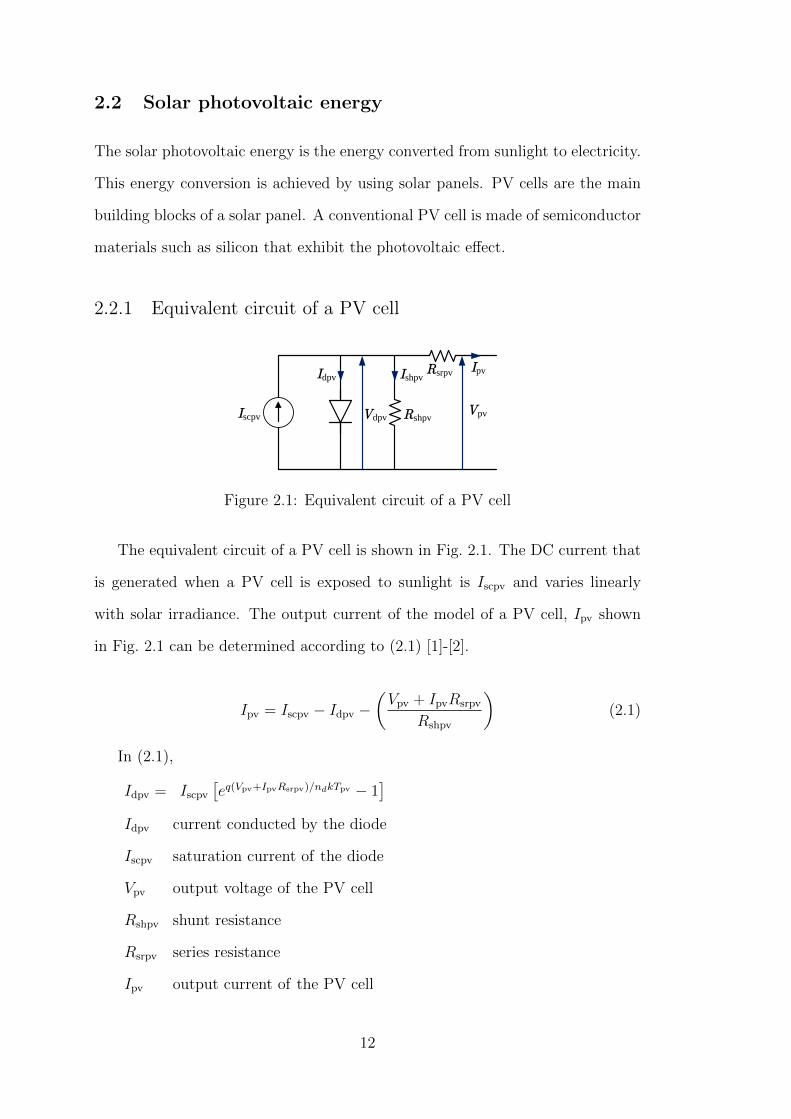
Figure 2.1: Equivalent circuit of a PV cell
The equivalent circuit of a PV cell is shown in Fig. 2.1. The DC current that
is generated when a PV cell is exposed to sunlight is Iscpv and varies linearly
with solar irradiance. The output current of the model of a PV cell, Ipv shown
in Fig. 2.1 can be determined according to (2.1) [1]-[2].
Ipv = Iscpv − Idpv −(Vpv + IpvRsrpv
Rshpv
)(2.1)
In (2.1),
Idpv = Iscpv
[eq(Vpv+IpvRsrpv)/ndkTpv − 1
]Idpv current conducted by the diode
Iscpv saturation current of the diode
Vpv output voltage of the PV cell
Rshpv shunt resistance
Rsrpv series resistance
Ipv output current of the PV cell
12
q electron charge (1.602× 10⁻¹⁹ As)
nd diode quality factor (1 < n < 2)
k Boltzmann′s constant (1.38× 10⁻²³ J/K)
Tpv absolute temperature (in K)
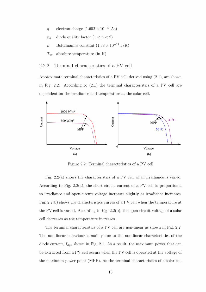
2.2.2 Terminal characteristics of a PV cell
Approximate terminal characteristics of a PV cell, derived using (2.1), are shown
in Fig. 2.2. According to (2.1) the terminal characteristics of a PV cell are
dependent on the irradiance and temperature at the solar cell.
Voltage
Cur
rent
Cur
rent
Voltage
1000 W/m2
800 W/m2
50 0C
30 0C
MPP
MPP
(a) (b)
0
Figure 2.2: Terminal characteristics of a PV cell
Fig. 2.2(a) shows the characteristics of a PV cell when irradiance is varied.
According to Fig. 2.2(a), the short-circuit current of a PV cell is proportional
to irradiance and open-circuit voltage increases slightly as irradiance increases.
Fig. 2.2(b) shows the characteristics curves of a PV cell when the temperature at
the PV cell is varied. According to Fig. 2.2(b), the open-circuit voltage of a solar
cell decreases as the temperature increases.
The terminal characteristics of a PV cell are non-linear as shown in Fig. 2.2.
The non-linear behaviour is mainly due to the non-linear characteristics of the
diode current, Idpv shown in Fig. 2.1. As a result, the maximum power that can
be extracted from a PV cell occurs when the PV cell is operated at the voltage of
the maximum power point (MPP). As the terminal characteristics of a solar cell
13
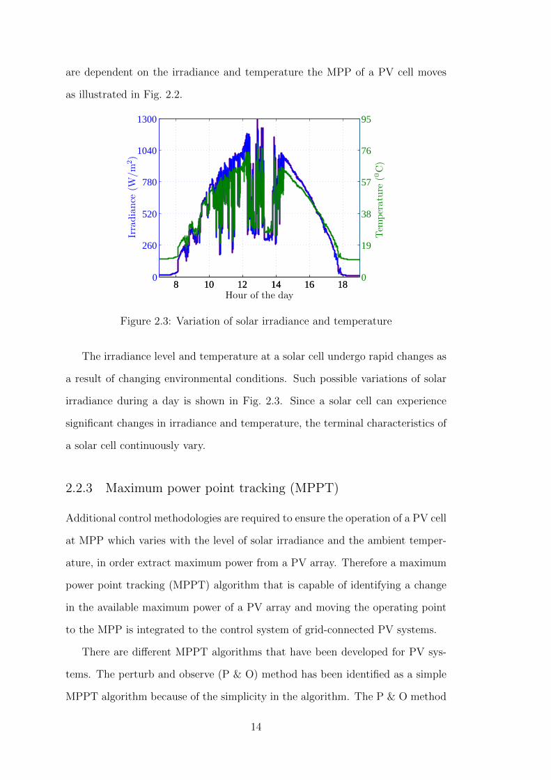
are dependent on the irradiance and temperature the MPP of a PV cell moves
as illustrated in Fig. 2.2.
8 10 12 14 16 180
260
520
780
1040
1300Irradiance
(W/m
2)
8 10 12 14 16 180
19
38
57
76
95
Tem
perature
(0C)
Hour of the day
Figure 2.3: Variation of solar irradiance and temperature
The irradiance level and temperature at a solar cell undergo rapid changes as
a result of changing environmental conditions. Such possible variations of solar
irradiance during a day is shown in Fig. 2.3. Since a solar cell can experience
significant changes in irradiance and temperature, the terminal characteristics of
a solar cell continuously vary.
2.2.3 Maximum power point tracking (MPPT)
Additional control methodologies are required to ensure the operation of a PV cell
at MPP which varies with the level of solar irradiance and the ambient temper-
ature, in order extract maximum power from a PV array. Therefore a maximum
power point tracking (MPPT) algorithm that is capable of identifying a change
in the available maximum power of a PV array and moving the operating point
to the MPP is integrated to the control system of grid-connected PV systems.
There are different MPPT algorithms that have been developed for PV sys-
tems. The perturb and observe (P & O) method has been identified as a simple
MPPT algorithm because of the simplicity in the algorithm. The P & O method
14
needs only one sensor. The P & O method has been identified as a slow tracking
algorithm compared to other available MPPT algorithms discussed in the litera-
ture. Sometimes, the P & O method fails in the presence of rapid variations of
the environmental conditions [3]. The continuous oscillations around the MPP is
a major drawback of the P & O method.
The next advanced MPPT algorithm is the incremental conductance (InC)
method. The InC method tracks the MPP quickly and accurately compared to
the P & O method [4]. In the InC method, once an MPP is found, theoretically
there are no oscillations around that point, as in the P & O method, until the
MPP changes due to variations in available solar irradiance and atmospheric
temperature. The InC method requires output current and voltage feedback of the
PV array. Hence a current sensor and a voltage sensor are needed to implement
the InC method. It is one sensor more than that is needed to implement the
P & O method. The InC method is a reasonably accurate, less complex and
easily implementable MPPT algorithm compared to quite sophisticated MPPT
algorithms that are discussed in recently published literature.
2.3 Power converters for integrating PV systems to the
grid
PV arrays are inherently DC power sources. Therefore, to integrate such systems
to an AC power distribution system, DC power from a PV array should be con-
verted to AC power. In order to perform the DC to AC power conversion, power
electronic converter systems are required. These utility interconnected power
electronic converter systems that convert DC power to AC power are categorised
based on the application, operation and control.
The authors of [5] categorise converters that interface PV systems to the
grid according to different power electronic circuit configurations presented in
Fig. 2.4 as a summary. The PV array configuration1 and the nominal voltage
1Mainly the open circuit voltage of the PV array.
15

Isolation TF on low frequency side
Isolation TF on high frequency side
PV Inverters
With DC-DC converter
Without DC-DC converter
With isolation TF
Without isolation TF
With isolation TF
Without isolation TF
Figure 2.4: Different configurations of power electronic converters that interfacePV systems to the grid
of the AC grid to which the PV system is connected, determines the necessity
of having a DC-DC power conversion stage to provide a suitable DC voltage for
the inverter stage2. The DC-DC power conversion stages can be eliminated with
careful selection of the PV array to closely match with the required DC voltage
required for the inverter ultimately leading to higher efficiency [5]. This may
not be always possible with small capacity PV installations which may need to
boost the output voltage of the PV array in order to achieve the required DC
side voltage of a PV system. In such situations a DC-DC boost converter can be
used to boost the output voltage of the PV array as suitable for integrating to
the grid.
Generally, galvanic isolation of inverters is considered to be a safety require-
ment. However, standards for grid connected energy systems via inverters permit
the elimination of such isolation, provided the inverters are carefully designed to
mitigate the problems with DC current injection, islanding, flicker and harmonics
[6], [7], [8], [9] and [10]. Since an isolation transformer introduces increased losses
and also adds to the cost of a PV system [11], [12], converters (inverters) without
galvanic isolation are usually preferred for relatively small domestic rooftop PV
installations.
Categories of converters can be grouped according to the commutation process
used in the design; as either line commutated converters or force commutated
converters. The latter is applicable in utility interactive systems such as grid-
2This refers to DC to AC power conversion.
16
connected PV systems where limitations on the harmonic current injection are
required [9].
DC-AC converters can be further categorised based on voltage and current
waveforms at their DC-links as either; voltage source converters or current source
converters (CSC). In a VSC, DC-link terminals are connected in parallel with a
relatively large capacitor and hence simulates characteristics of a voltage source.
The DC-link voltage of a VSC retains the same polarity and the direction of
the converter average power flow as determined by the polarity of the DC-link
current. In a CSC, the DC-link is connected in series with a relatively large
reactor and hence simulates the characteristics of a current source. The DC-link
current retains the same polarity and the direction of the average power flow
is determined by the DC-link voltage. In order to be able to fully control the
power flow through a CSC, it should be made from fully controllable bipolar
power electronic switches. Currently, such switches are commercially available
only for very high power converter markets. Unlike in a CSC, power flow of a
VSC can be fully controlled if the converter is made of reverse conducting power
electronic switches. Such power electronic switches are commercially available as
IGBT or MOSFET and those are suitable for low power converter applications
[13]. Therefore, VSCs have become the most suitable type of power electronic
converters to interface low power PV systems to the grid.
2.4 Operation and control of a VSC
2.4.1 Basic operation of a VSC
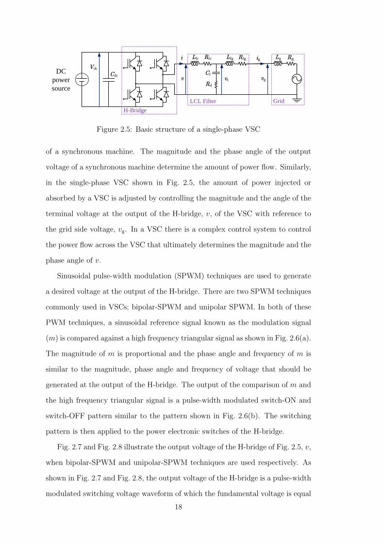
The basic structure of a single-phase VSC that interfaces a DC power source to
the grid is shown in Fig. 2.5. The single-phase VSC is made of an H-bridge3. In
Fig. 2.5, Cdc is the DC-link capacitor and Vdc is the DC-link voltage.
The control of power flow across a VSC is similar to the control of power flow
3This is also referred to as a full-bridge.
17
Grid
Lfc Lfg
Rd
Cf
Rfc Rfg ig
vg
LCL Filter
DC power source
H-Bridge
vcv
i
Cdc
Vdc
Lg Rg
Figure 2.5: Basic structure of a single-phase VSC
of a synchronous machine. The magnitude and the phase angle of the output
voltage of a synchronous machine determine the amount of power flow. Similarly,
in the single-phase VSC shown in Fig. 2.5, the amount of power injected or
absorbed by a VSC is adjusted by controlling the magnitude and the angle of the
terminal voltage at the output of the H-bridge, v, of the VSC with reference to
the grid side voltage, vg. In a VSC there is a complex control system to control
the power flow across the VSC that ultimately determines the magnitude and the
phase angle of v.
Sinusoidal pulse-width modulation (SPWM) techniques are used to generate
a desired voltage at the output of the H-bridge. There are two SPWM techniques
commonly used in VSCs; bipolar-SPWM and unipolar SPWM. In both of these
PWM techniques, a sinusoidal reference signal known as the modulation signal
(m) is compared against a high frequency triangular signal as shown in Fig. 2.6(a).
The magnitude of m is proportional and the phase angle and frequency of m is
similar to the magnitude, phase angle and frequency of voltage that should be
generated at the output of the H-bridge. The output of the comparison of m and
the high frequency triangular signal is a pulse-width modulated switch-ON and
switch-OFF pattern similar to the pattern shown in Fig. 2.6(b). The switching
pattern is then applied to the power electronic switches of the H-bridge.
Fig. 2.7 and Fig. 2.8 illustrate the output voltage of the H-bridge of Fig. 2.5, v,
when bipolar-SPWM and unipolar-SPWM techniques are used respectively. As
shown in Fig. 2.7 and Fig. 2.8, the output voltage of the H-bridge is a pulse-width
modulated switching voltage waveform of which the fundamental voltage is equal
18
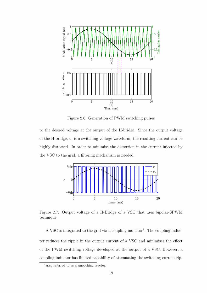
0 5 10 15 20−1
−0.5
0
0.5
1
Modulationsignal
(m)
0 5 10 15 20−1
−0.5
0
0.5
1
Triangularcarrier
(a)
0 5 10 15 20
OFF
ON
Switchingpattern
(b)Time (ms)
Figure 2.6: Generation of PWM switching pulses
to the desired voltage at the output of the H-bridge. Since the output voltage
of the H-bridge, v, is a switching voltage waveform, the resulting current can be
highly distorted. In order to minimise the distortion in the current injected by
the VSC to the grid, a filtering mechanism is needed.
0 5 10 15 20
−Vdc
0
Vdc
Time (ms)
v
v
vo
Figure 2.7: Output voltage of a H-Bridge of a VSC that uses bipolar-SPWMtechnique
A VSC is integrated to the grid via a coupling inductor4. The coupling induc-
tor reduces the ripple in the output current of a VSC and minimises the effect
of the PWM switching voltage developed at the output of a VSC. However, a
coupling inductor has limited capability of attenuating the switching current rip-
4Also referred to as a smoothing reactor.
19
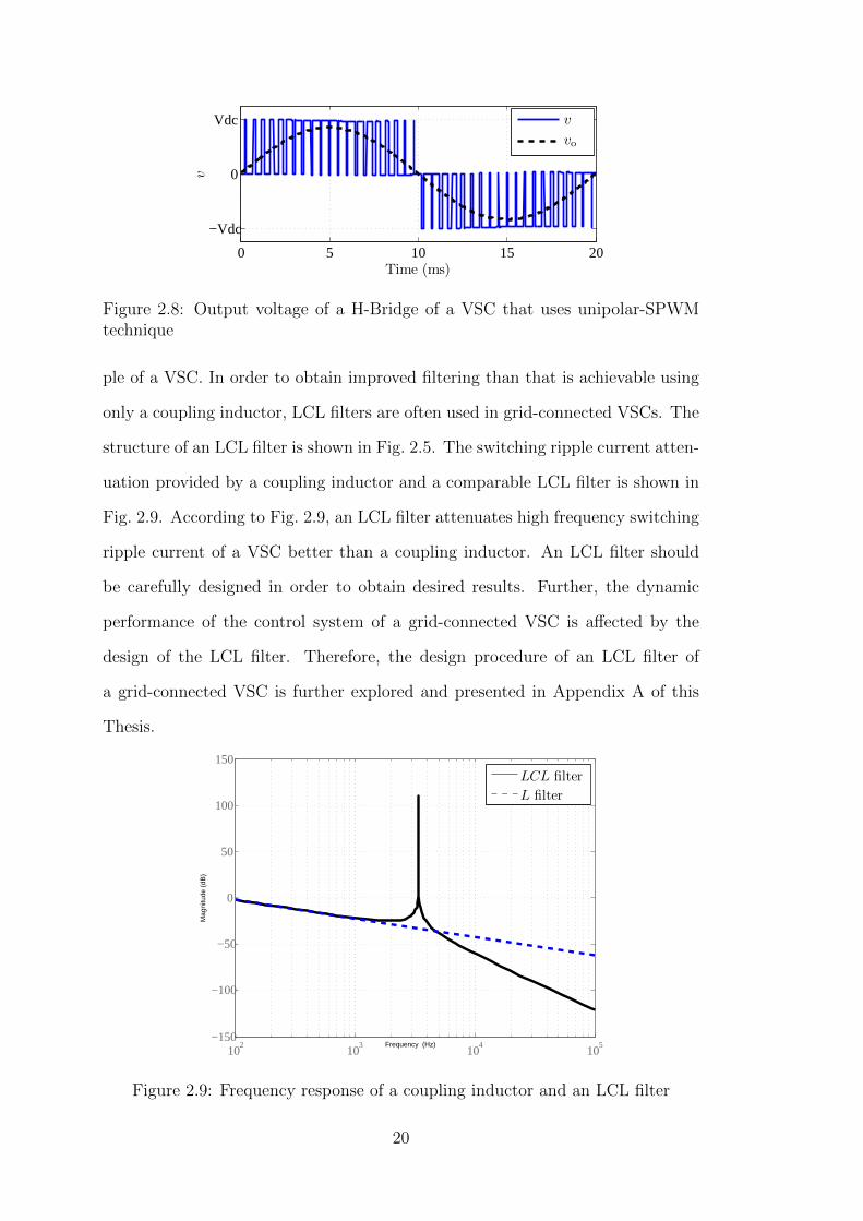
0 5 10 15 20
−Vdc
0
Vdc
Time (ms)
v
v
vo
Figure 2.8: Output voltage of a H-Bridge of a VSC that uses unipolar-SPWMtechnique
ple of a VSC. In order to obtain improved filtering than that is achievable using
only a coupling inductor, LCL filters are often used in grid-connected VSCs. The
structure of an LCL filter is shown in Fig. 2.5. The switching ripple current atten-
uation provided by a coupling inductor and a comparable LCL filter is shown in
Fig. 2.9. According to Fig. 2.9, an LCL filter attenuates high frequency switching
ripple current of a VSC better than a coupling inductor. An LCL filter should
be carefully designed in order to obtain desired results. Further, the dynamic
performance of the control system of a grid-connected VSC is affected by the
design of the LCL filter. Therefore, the design procedure of an LCL filter of
a grid-connected VSC is further explored and presented in Appendix A of this
Thesis.
102
103
104
105
−150
−100
−50
0
50
100
150
Mag
nitu
de (
dB)
Frequency (Hz)
LCL filter
L filter
Figure 2.9: Frequency response of a coupling inductor and an LCL filter
20

2.4.2 Four-quadrant operation of a VSC
A VSC can be controlled to inject or absorb real and reactive power to the grid.
The real and reactive power exchange between a VSC and an AC system can be
controlled independently. Therefore, any combination of real power injection or
absorption along with reactive power injection or absorption is achievable [14].
Such an operational capability of a VSC is referred to as four-quadrant operation
and that can be represented in four quadrants of a Cartesian coordinate system
as shown in Fig. 2.10. The sample operating scenarios of a VSC indicated in
Fig. 2.10 are as follows.
PCC
Pg
Qg
XgRg
Pg
Qg
VSC
Quadrant 2PCC
Pg
Qg
VSC
PCC
Pg
Qg
XgRgVSCPCC
Pg
Qg
VSC
Grid
Grid
XgRg
Grid
XgRg
Grid
EnergyStorage SolarPhotovoltaic
Quadrant 1
Quadrant 3 Quadrant 4
Figure 2.10: Four-quadrant operation of a VSC
• Quadrant 1 - Charging a battery bank while operating at a leading power
factor.
• Quadrant 2 - A PV system operating at a leading power factor.
• Quadrant 3 - A PV system operating at a lagging power factor.
• Quadrant 4 - Charging a battery bank while operating at a lagging power
factor.
Fig. 2.10 introduces counting directions used in this Thesis for active and re-
active power flow outputs of a grid-connected VSC. In this Thesis, active power
21

injected and reactive power absorbed (inductive operation) by a VSC are counted
negative and active power absorbed and reactive power injected (capacitive op-
eration) by a VSC are counted positive.
The real and reactive power injection or absorption by a VSC is limited only
by the converter current carrying capacity. The operating limits of an ideal
VSC are illustrated in Fig. 2.11. In Fig. 2.11, the kVA rating of the converter
is represented by a vector of magnitude Sr. As per Fig. 2.11, when a VSC is
injecting active power Pg to the grid, the VSC is able to either absorb Qg amount
of reactive power from the grid or inject Qg amount of reactive power to the grid.
This means that a VSC is capable of absorbing or injecting the same magnitude
of reactive power for a given Pg. It is evident from Fig. 2.11 that when active
power is zero, the converter is capable of operating at its maximum reactive power
limit that is equal to the rated kVA capacity of the VSC.
P
Q
Sr
-Pg
+Qg
-Qg
Figure 2.11: Operating limits of an ideal VSC
2.4.3 Control systems in a VSC
A VSC can be categorised based on the control philosophy as either voltage-
controlled or current-controlled. In a voltage-controlled VSC, the real and reac-
tive power output are controlled by adjusting the phase angle and the magnitude
22

of the output voltage of the VSC relative to the PCC voltage. There are fewer
control loops in this type of a VSC and there is no closed-loop to control its
output current. Hence the VSC is not protected by the control system against
over current.
In a current-controlled VSC, the output current of the VSC is controlled by a
closed-loop current controller. Hence, such a VSC is inherently protected against
over current. In a current-controlled VSC, the control of the active and reactive
power outputs is achieved by controlling the output current by adjusting the
magnitude and phase angle of the output voltage of the VSC with respect to the
grid voltage. Since a current-controlled VSC provides better protection against
over current, avoiding disconnection in such situations, these are increasingly
being used to integrate PV systems to the grid. In a current controlled VSC, the
closed-loop current controller and grid synchronisation mechanism are the two
main control systems.
Current controller of a VSC
In three-phase VSCs, synchronous reference frame5 current controllers are widely
used. Such a current controller provides flexibility by independently controlling
the injected or absorbed active and reactive power. The synchronous reference
frame current controller requires the transformation of measured AC signals, out-
put current and voltage of a VSC, into DC signals using the Park Transformation.
The measured output current and voltage of a VSC that is transformed to DC
signals are the inputs to a synchronous reference frame current controller. These
DC signals are passed through a proportional and integral (PI) regulator6 in the
synchronous reference frame current controllers and generate control inputs to
the PWM generator of the VSC in synchronous reference frame.
The application of a synchronous reference frame current controller to a single-
5Also known as rotating frame or dq frame.6A PI regulator is used to achieve zero steady-state error since such a regulator provides an
infinite gain for DC signals.
23
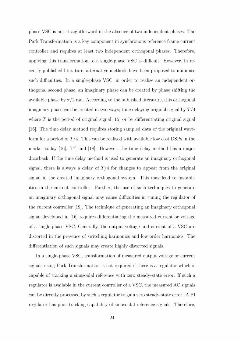
phase VSC is not straightforward in the absence of two independent phases. The
Park Transformation is a key component in synchronous reference frame current
controller and requires at least two independent orthogonal phases. Therefore,
applying this transformation to a single-phase VSC is difficult. However, in re-
cently published literature, alternative methods have been proposed to minimise
such difficulties. In a single-phase VSC, in order to realise an independent or-
thogonal second phase, an imaginary phase can be created by phase shifting the
available phase by π/2 rad. According to the published literature, this orthogonal
imaginary phase can be created in two ways; time delaying original signal by T/4
where T is the period of original signal [15] or by differentiating original signal
[16]. The time delay method requires storing sampled data of the original wave-
form for a period of T/4. This can be realised with available low cost DSPs in the
market today [16], [17] and [18]. However, the time delay method has a major
drawback. If the time delay method is used to generate an imaginary orthogonal
signal, there is always a delay of T/4 for changes to appear from the original
signal in the created imaginary orthogonal system. This may lead to instabil-
ities in the current controller. Further, the use of such techniques to generate
an imaginary orthogonal signal may cause difficulties in tuning the regulator of
the current controller [19]. The technique of generating an imaginary orthogonal
signal developed in [16] requires differentiating the measured current or voltage
of a single-phase VSC. Generally, the output voltage and current of a VSC are
distorted in the presence of switching harmonics and low order harmonics. The
differentiation of such signals may create highly distorted signals.
In a single-phase VSC, transformation of measured output voltage or current
signals using Park Transformation is not required if there is a regulator which is
capable of tracking a sinusoidal reference with zero steady-state error. If such a
regulator is available in the current controller of a VSC, the measured AC signals
can be directly processed by such a regulator to gain zero steady-state error. A PI
regulator has poor tracking capability of sinusoidal reference signals. Therefore,
24
in order to track sinusoidal signals with zero steady-state error, a stationary
frame regulator named proportional resonant (PR) controller has been proposed
in [20]. This regulator is readily applicable for both three phase and single phase
VSCs. A PR regulator achieves zero steady-state error for signals at the designed
frequency. Hence, signal transformation from AC to DC and back to AC, as is
required for a synchronous reference frame current controller, is not necessary.
Furthermore, the formation of an imaginary orthogonal signal is not necessary
in stationary frame current controllers. Hence, the dynamic performance of a
stationary frame current controller in a single-phase VSC is superior compared
to the synchronous frame current controller of a single-phase VSC.
Grid synchronisation of a VSC
In a VSC, a grid synchronisation mechanism is used for synchronising the VSC
to the grid. Further, in a current-controlled VSC, the grid synchronisation mech-
anism is also used for generating an accurate current reference signal in order to
inject the desired amount of active and reactive power to the grid. There are
different grid synchronisation mechanisms that are used to synchronise a VSC to
the grid according to recently published literature. Depending on the application
and type of current controller used in the VSC, a suitable grid synchronisation
method should be chosen.
One of the simplest grid synchronisation methods is the voltage zero crossing
detection. Since voltage zero crossings occur every half a cycle, the dynamic per-
formance of the voltage zero crossing detection method is quite low [21]. However,
the voltage zero crossing detection method for synchronising a VSC to the grid
can fail in the presence of harmonics in the grid because of multiple zero crossings
[22].
Other grid synchronisation methods are mostly based on a phase-locked-loop
(PLL). Among different PLL methods, synchronous reference frame based PLL
(s-PLL) has been identified as suitable for a single-phase VSC [21], [23]. In the
25

s-PLL, the peak value of the measured grid voltage can be obtained easily.
2.5 Grid-connected PV system
LV power grids in Australia are undergoing significant changes with the connec-
tion of a large number of small capacity PV systems. Small scale PV systems
(0 − 10 kW) are the type of renewable energy units that are mostly connected
to these networks. Commercially attractive rebates and concession schemes that
were introduced by the Australian government for installing small scale PV sys-
tems along with price reductions in PV panels and power electronic converter
systems, are the main reasons for the increased number of grid-connected small
scale PV systems in LV power grids. The majority of small scale PV systems are
domestic roof-top type installations and are generally single-phase systems [24].
The basic structure of a grid-connected single-phase PV system is shown in
Fig. 2.12. This is a generic representation of a domestic roof-top PV system. The
PV system consists of a DC-DC converter, a VSC and an LCL filter. The PCC
is where the PV system is connected to the grid.
Cpv
Ipv
Cdc
Idc
VdcVpv
i
v vg
DC-DC Boost Converter
Voltage Source Converter
LCL Filter Distribution Grid
PCC
Ppv Pdc Pc , Qc
Photovoltaic Array
Pg , Qg
ig
Xg Rg
Lfc Lfg
RdCf
Rfc RfgLdc
vs
Figure 2.12: Basic structure of a grid-connected PV system
In the grid-connected PV system shown in Fig. 2.12, the DC-DC converter
steps up or steps down the output voltage of the PV array to a suitable level at
the output of the DC-DC converter. An MPPT algorithm determines the MPP
of the PV array at a given time and the DC-DC converter is controlled in such
a way that the PV array is operated at the MPP. The output of the MPPT
algorithm is an input to the controller of the DC-DC converter.
26
The PV system shown in Fig. 2.12 is integrated to the grid via a VSC. A VSC
with an ability to control output voltage magnitude and phase angle with refer-
ence to the voltage at the PCC and is able to operate in all four quadrants, pro-
vides a significant flexibility in controlling the active and reactive power injected
or absorbed by or from the grid. Therefore, VSCs are becoming more attrac-
tive in PV grid integration especially with the additional capability of providing
reactive power support, voltage regulation [25] and managing battery storage.
The output power from a PV array is a function of solar irradiance and ambi-
ent temperature. Since solar irradiance and ambient temperature vary, the power
output of a PV array is not constant. If the grid-connected PV system shown
in Fig. 2.12 is controlled to inject a constant amount of power to the grid at
times when power level varies at the PV array, the DC-link capacitor, Cdc may
be charged or discharged affecting the DC-link voltage, Vdc. However, maintain-
ing a constant DC-link voltage is necessary in order to minimise the appearance
of low-order harmonics at the output of the VSC as a result of PWM switching
of the power electronic switches of the VSC. Therefore, in a grid-connected PV
system a controller is used to control the DC-link voltage at a suitable level by
controlling the active power flow of the PV system.
2.6 Impact of the integration of multiple PV systems on
an LV power grid
Operational or power quality problems may occur in LV power grids as a result
of integration of a large number of small scale multiple PV systems. The inte-
gration of small scale multiple PV systems means that LV power grids may have
an increased susceptibility to voltage fluctuations due to injected active power
variations from the PV systems, depending on conditions such as the time of
day and weather. Such variations in output power can cause voltage fluctuations
(either slow or fast) in LV power grids where concentrated PV installations exist
27
[26]. Since PV systems are interfaced to LV power grids through power electronic
converters, which is equivalent to a condition where there is no mechanical iner-
tia, the speed of response of PV systems in relation to reduction or increase in
available power can be very fast indeed [27]. Therefore, in a power distribution
feeder to which multiple PV systems are integrated there is a possibility that
feeder voltage can vary significantly as a result of variable power injections from
PV systems.
There may be operational and control interactions between PV systems or
with the grid if multiple PV systems are integrated into the LV power grid [25],
[28], [22] and [29]. These interactions may cause unintentional tripping of PV
systems, possibly making the grid unstable or a system may fail to disconnect
when it is necessary to do so, creating a hazardous situation. Therefore, possible
mechanisms and causes for operational and control interactions should be identi-
fied first, to propose any mitigation techniques to avoid undesirable interactions
between multiple PV systems for a stable operation of LV power grids. Further-
more, there can be potential instabilities within a grid-connected PV system if
the operating point of the PV array is moved towards the constant current region
of the characteristic curve of a PV array [30]. The prior identification of the
possibility of occurring such problems in an LV power grid containing multiple
PV systems is critical for both power utilities and PV system designers.
In order to investigate possible rapid and slow voltage fluctuations at the
grid interface, operational and control interactions in the presence of multiple
grid-connected PV systems and also to evaluate potential instabilities, a detailed
model of a grid-connected single-phase PV system is necessary. The knowledge
on component level modelling of a grid-connected PV system is available with
recently published literature for both 3-phase and single-phase systems [31],[32].
However, a complete model of a grid-connected single-phase PV system with
associated control design methodologies is not readily available. Therefore, the
development of a detailed model of a grid-connected single-phase two-stage PV
28
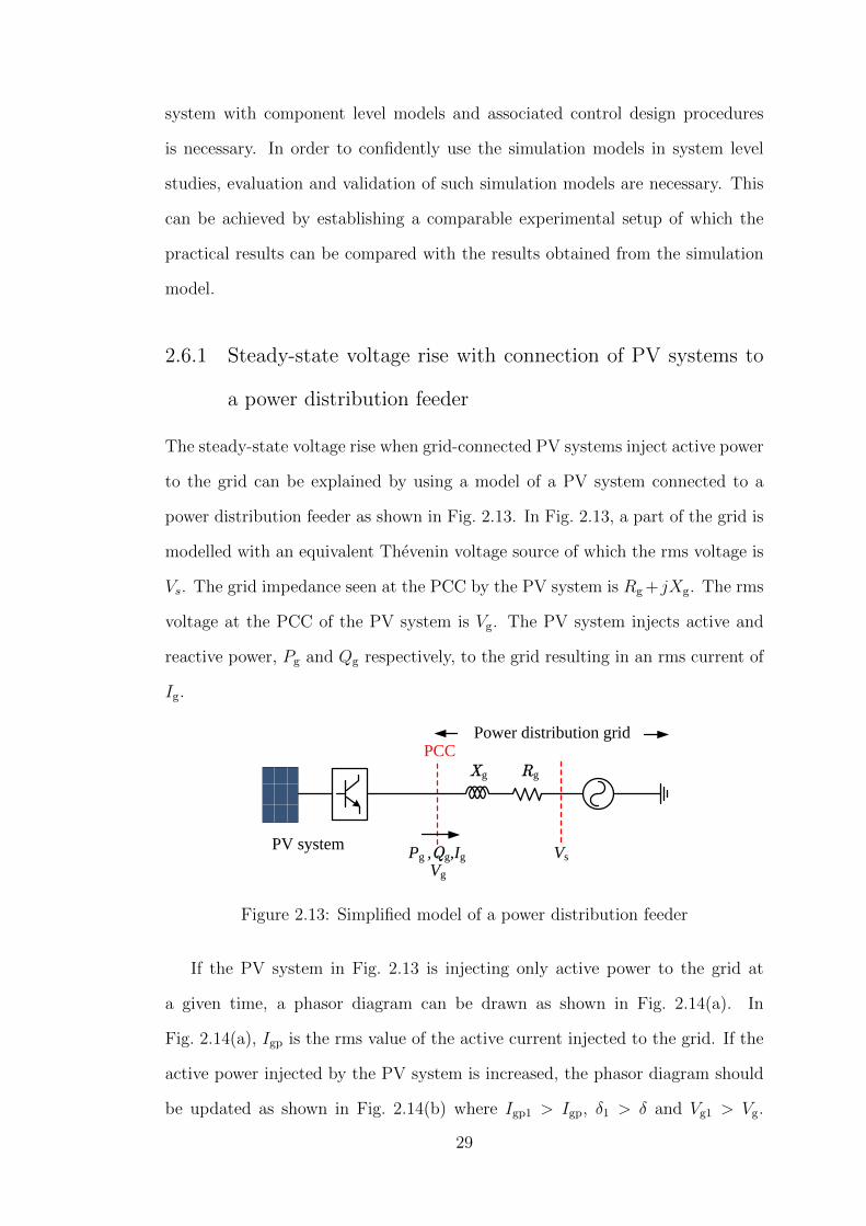
system with component level models and associated control design procedures
is necessary. In order to confidently use the simulation models in system level
studies, evaluation and validation of such simulation models are necessary. This
can be achieved by establishing a comparable experimental setup of which the
practical results can be compared with the results obtained from the simulation
model.
2.6.1 Steady-state voltage rise with connection of PV systems to
a power distribution feeder
The steady-state voltage rise when grid-connected PV systems inject active power
to the grid can be explained by using a model of a PV system connected to a
power distribution feeder as shown in Fig. 2.13. In Fig. 2.13, a part of the grid is
modelled with an equivalent Thevenin voltage source of which the rms voltage is
Vs. The grid impedance seen at the PCC by the PV system is Rg +jXg. The rms
voltage at the PCC of the PV system is Vg. The PV system injects active and
reactive power, Pg and Qg respectively, to the grid resulting in an rms current of
Ig.
Xg
Vs
Power distribution gridPCC
Pg ,Qg,IgVg
Rg
PV system
Figure 2.13: Simplified model of a power distribution feeder
If the PV system in Fig. 2.13 is injecting only active power to the grid at
a given time, a phasor diagram can be drawn as shown in Fig. 2.14(a). In
Fig. 2.14(a), Igp is the rms value of the active current injected to the grid. If the
active power injected by the PV system is increased, the phasor diagram should
be updated as shown in Fig. 2.14(b) where Igp1 > Igp, δ1 > δ and Vg1 > Vg.
29
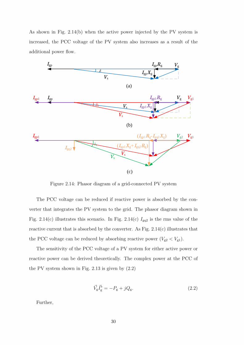
As shown in Fig. 2.14(b) when the active power injected by the PV system is
increased, the PCC voltage of the PV system also increases as a result of the
additional power flow.
VgIgp
IgpXgδ
δ1
Vs
IgpRg
IgpIgp1
Vs
Vs Igp1Xg
Igp1Rg Vg Vg1
Igp1
Igq2δ2
VsVs
Vg1Vg2(Igp1Rg-Igq2Xg)
(Igp1Xg+Igq2Rg)
(a)
(b)
(c)
Figure 2.14: Phasor diagram of a grid-connected PV system
The PCC voltage can be reduced if reactive power is absorbed by the con-
verter that integrates the PV system to the grid. The phasor diagram shown in
Fig. 2.14(c) illustrates this scenario. In Fig. 2.14(c) Igq2 is the rms value of the
reactive current that is absorbed by the converter. As Fig. 2.14(c) illustrates that
the PCC voltage can be reduced by absorbing reactive power (Vg2 < Vg1).
The sensitivity of the PCC voltage of a PV system for either active power or
reactive power can be derived theoretically. The complex power at the PCC of
the PV system shown in Fig. 2.13 is given by (2.2)
~Vg~I∗g = −Pg + jQg. (2.2)
Further,
30

~Vg − ~Vs = ~Ig(Rg + jXg). (2.3)
From (2.2) and (2.3),
~Vg − ~Vs =
(−Pg + jQg
~Vg
)∗(Rg + jXg),
~Vg − ~Vs =(−Pg − jQg)(Rg + jXg)
~V ∗g. (2.4)
If the phase angle deviation of ~Vs with reference to ~Vg is assumed negligible
and considering ~Vg to be the reference phasor, (2.4) can be simplified as,
Vg − Vs =−PgRg +QgXg
Vg
,
∆Vg =−PgRg +QgXg
Vg
, (2.5)
where ∆Vg = Vg − Vs which is the steady-state voltage rise. As per the
simplified expression (2.5) the steady-state voltage rise, ∆Vg increases as active
power injected to the grid, Pg7 increases and ∆Vg can be decreased by absorbing
reactive power from the grid. If active power injected by a PV system can be
controlled, ∆Vg can also be controlled by controlling both active power, Pg and
reactive power, Qg injected by the PV system.
2.6.2 Voltage level variations in an LV power grid integrated with
multiple PV systems
The integration of multiple PV systems to an LV power grid is now known to
cause grid voltage rise problem [33], [34] and [35]. The grid voltage may exceed the
specified highest voltages in the applicable standards such as Australian Standard
7Note that active power injection to the grid is counted negative.
31
AS4777.2 [7] and IEEE Standard 929-2000 [9], especially in situations when the
power generation from PV systems is at a peak and the load on the grid is at
a minimum. According to Australian Standard AS4777.2 [7] the maximum grid
voltage up to which a PV system can remain connected is 230 V + 10%. The
disconnection of PV systems from the grid leads to loss of energy yield from the
installed PV systems and income for the resource owner. If the voltage regulation
at the PCC of the PV system is possible by any means, increased and continuous
active power injection can be achieved from the connected PV systems.
In a power distribution feeder where multiple PV systems are integrated, there
is a possibility for reverse power flow in the feeder. This scenario depends on the
load demand and available power from PV systems. Conventional distribution
voltage regulation devices such as fixed capacitors, tap changers at distribution
transformers and step voltage regulators are not capable of regulating the feeder
voltage in such a situation [9]. However, if dynamic voltage regulators are added
to the system, conventional devices can be properly coordinated to operate the
grid within safe limits [36].
Impact on the voltage levels of an LV power grid integrated with a large
number of PV systems can be quite significant. High penetration of PV systems
may cause over-voltages or severe voltage fluctuations in the grid. Therefore, in
order to operate a grid within safe margins while harnessing the maximum active
power from PV, fast and dynamic voltage regulating systems must be installed
and operated in the grid.
2.7 Voltage control in an LV power grid integrated with
multiple PV systems
The PCC voltage of a PV system is sensitive to both active and reactive power
injected by a PV system and the grid impedance according to (2.5). PV systems
are integrated to the grid via power electronic converters and, more specifically,
32
often via VSCs [5], [37]. A VSC is capable of operating in all four quadrants when
designed appropriately and such systems have been shown to be a fast, efficient
and cost effective means of regulating voltage and power factor for nearby loads
[38], [39], [40] and [41]. Further, the active and reactive power outputs of a PV
system that is integrated to the grid via a VSC can be controlled independently.
Therefore, fast voltage control in an LV power grid can be achieved by PV systems
integrated to the grid via VSCs. Therefore, it is beneficial for both utilities and
consumers to utilise the added value capabilities of modern PV systems to improve
power quality in the grid.
The Australian and IEEE standards applicable for grid-integrated PV sys-
tems, Australian Standard AS4777.1 [7] and IEEE Standard 1547-2003 [10] re-
spectively, permit the use of PV systems for the purpose of voltage support but
do not permit active voltage regulation at the PCC of a PV system. However,
in Australian Standard AS4777.1 [7] there is a provision given for active voltage
regulation by grid-integrated PV system. According to that particular standard,
the utility who owns the LV power grid to which a PV system is integrated has
the authority to permit active voltage regulation by the PV system.
The static voltage support methodologies provided by PV systems, such as
constant and variable power factor, have been identified as inefficient as these
methods may cause additional reactive power flow in the grid even when the grid
voltage is well within the limits and may lead to overloading of the distribution
transformer [33]. A droop based reactive power control method (referred to as
Q(U) method) has been proposed in [42] which aims to minimise the drawbacks of
the static reactive power control methodologies. In order to implement the Q(U)
reactive power control method effectively, grid specific studies or additional deci-
sion making control algorithms such as the fuzzy logic based adaptive controller
presented in [43] are necessary. Further, Q(U) reactive power control method
is not able to maintain the PCC voltage of a PV system below the maximum
allowable voltage all the time.
33

The PCC voltage of a PV system can be regulated by a closed-loop controller
that dynamically controls the reactive power response of the PV system. Such a
controller has been identified as an efficient way of regulating PCC voltage with
reactive power [33]. The ability to regulate the PCC voltage with a closed-loop
controller that dynamically controls the reactive power injected to the grid by the
PV system is limited. This limitation is mainly due to the limited rating of the
VSC that interfaces the PV system to the grid. When the PV system is injecting
a certain amount of active power to the grid, only the excess capacity of the
VSC, if any, can be used to inject/absorb reactive power. The available limited
reactive power capacity of the PV system at a given time may not be adequate
to regulate the PCC voltage at 230 V + 10% or at any other specified voltage
reference depending on the voltage sensitivity of the PCC. In such a situation
active power curtailing is an option to control the PCC voltage in the absence of
energy storage systems [35], [44] and [45]. Similar to closed-loop reactive power
control of a PV system, closed-loop active power control can be proposed as an
effective way of regulating PCC voltage of a PV system.
In the published literature, little attention has been given to adequate tech-
nical details and guidelines for practically implementing closed-loop controllers
that control the active and reactive power response of a PV system in order to
regulate the PCC voltage of the PV system. Therefore, detailed design proce-
dures of closed-loop active and reactive power controllers that are capable of
dynamically regulating the PCC voltage of a grid-connected PV system need to
be developed. The sensitivity of active and reactive power controllers to the gains
of the controllers and the grid impedance should be evaluated. Once closed-loop
active and reactive power controllers are developed, by combining the operation
of closed-loop active and reactive power controllers, novel operating strategies
can be proposed for grid-connected PV systems. The robustness of the designed
closed-loop active and reactive power controllers and the feasibility of implement-
ing novel operating strategies for grid-connected PV systems should be validated
34

experimentally.
2.8 Application of distribution static synchronous com-
pensator (DSTATCOM)
A DSTATCOM is a VSC which is primarily used to exchange reactive power with
the AC system. In power distribution systems, DSTATCOMs are mainly used for
voltage regulation [13], [14]. A DSTATCOM is usually operated as a shunt con-
nected static var compensator of which capacitive and inductive output current
can be controlled independent of the AC system voltage. Hence a DSTATCOM
can be used to either provide voltage support or active voltage control in an LV
power grid.
A PV system that is integrated to the grid via a VSC can be operated as
a DSTATCOM. The active power injection by a PV system is possible only at
times when there is adequate solar irradiance. When there is not enough solar
irradiance8 ideally the rated capacity of the VSC that interfaces PV system to
the grid can be operated as a DSTATCOM. Therefore, PV systems that are
interfaced to the grid via VSCs can be fully deployed to provide voltage support
or active voltage control at times when there is not enough solar irradiance to
generate electrical power, by operating those as DSTATCOMs.
The application of DSTATCOMs for distribution network voltage regulation
has been examined [46], [47] and [48]. Although this is the case, suitability of
using multiple DSTATCOMs for providing voltage support or grid voltage control
in a grid to which multiple PV systems are integrated has not been evaluated.
Therefore, identifying the suitability of using the DSTATCOM for providing volt-
age support or grid voltage control in a grid to which multiple PV systems are
integrated is necessary. Further, the development of control coordination strate-
gies for operation of multiple DSTATCOMs will also be beneficial.
8For an example, at night time.
35
2.9 Operational and control interactions between multi-
ple PV systems
In the presence of multiple PV units that are connected to an LV power grid,
there can be operational conflicts. These units may interfere or interact with
each other’s operation and control. Therefore, it is of utmost importance to iden-
tify the possible conflicts between different converter systems that would disturb
their smooth operation. Mitigation techniques and necessary design modifications
should be recognised. Algorithms must be developed to achieve ride-through ca-
pability of renewable resources and avoid unintentional shut down of PV systems
to avoid abrupt changes in the grid.
In an LV power grid to which multiple PV systems are integrated, the grid
voltage can be controlled by regulating the PCC voltage of each PV system [35],
[49], [34], [33] and [42]. A PV system that is integrated with a closed-loop PCC
voltage controller is able to regulate the PCC voltage of a PV system dynami-
cally at a set reference voltage with zero steady-state error by absorbing reactive
power from the grid. Such a controller has been identified as an efficient way of
regulating the PCC voltage of a PV system [33]. Therefore, multiple PV systems
that are connected to a grid and that are integrated with a closed-loop PCC
voltage controller can be used to control the grid voltage dynamically. However,
when multiple PV systems operate electrically close to each other while dynami-
cally controlling the grid voltage, there may be control interactions between PV
systems.
The control interactions between power system stabilisers (PSS) and flexible
AC transmission system (FACTS) devices operating in high voltage transmission
networks have been well investigated in the published literature [50], [51], [52],
[53] and [54]. However, there is only a limited number of published articles avail-
able on the control interaction between dynamic voltage control devices that are
connected to an LV power grid. This is an emerging topic of discussion amongst
36
researchers. The dynamic interaction between DSTATCOMs connected to a ra-
dial power distribution feeder is analysed in [55] and simulation results of control
interaction between PV systems are presented in [56]. In [55], the research scope
is limited to DSTATCOMs that are made of voltage controlled VSCs and the sen-
sitivity of the gains of controllers to the stability of the individual DSTATCOM
has been overlooked. The negative interaction between multiple PV systems
identified in [56] of PV systems interfaced to the grid via current controlled VSCs
does not appear if a dead-band is added to the PCC voltage controller of a PV
system.
Control and operational interaction between multiple PV systems can be iden-
tified using accurate simulation models and validated mathematical models. How-
ever, since such simulation and mathematical models are not readily available
those should be developed and validated. The development of such tools will
be beneficial for power utilities who are, at present, quite uncertain about the
impact, a high penetration of PV systems will have on the grid. Further, simu-
lation and mathematical models that will enable the identification of operational
and control interactions between PV systems will also enable the development
of proper coordination and control strategies which could be adopted for volt-
age control and reactive power compensation by PV systems while improving
system stability and efficiency. In order to develop such analytical tools, a thor-
ough knowledge on the operation and control of grid-integrated PV systems and
practical techniques used to establish control systems is necessary.
2.10 Control and coordination of the operation of multi-
ple PV systems
The operation of small scale PV systems is not currently monitored like in the
case of conventional large power generators, since the impact of such PV systems
is tolerable in existing power systems. However once multiple PV systems are
37

present in the grid, their collective impact on the system operation and control
will be significant. Therefore these units should be integrated with proper coor-
dination and control practices for acceptable operation of the grid. Further, it
is unclear whether or not all PV systems integrated to an LV power grid should
provide voltage support, or should there be a staged introduction of this support.
For staged introduction of voltage support, development of mechanisms for con-
veying the appropriate changes to control parameters in a coordinated and timely
manner will be necessary. The majority of existing LV power grids does not have
any established communication facilities with it. Therefore, initially, method-
ologies should be developed for proper coordination and control of multiple PV
systems without the use of communication infrastructure and later these devel-
oped methodologies should be extended as suitable for LV power grids integrated
with multiple PV systems in which communication infrastructure exists.
When a certain amount of active and reactive power is injected to the grid
by a PV system, the PCC voltage of the PV system is a function of the voltage
sensitivity at the PCC. Further, the voltage sensitivity at the PCC of a PV
system is a function of the grid impedance seen by the PV system at the PCC.
Therefore, in certain operating situations, the voltage at the PCC of a PV system
where voltage sensitivity is high may reach unacceptable high voltage levels while
the PCC voltages at locations of other PV systems connected to the grid are
lower. In such a situation, the PV system that is connected to the grid at a node
where voltage sensitivity is high may disconnect in order to comply with the
requirements of the Australian Standard AS477.2 [7] while other PV systems will
continue to operate. The discussed scenario highlights that in certain operating
situations, owners of PV systems whose PV systems are integrated to the grid
at nodes where voltage sensitivity is high are disadvantaged over the other PV
system owners whose PV systems are connected to the grid at nodes where voltage
sensitivity is less.
A droop based active power sharing methodology is proposed in [45] for PV
38
systems connected to a radial distribution feeder. Since the droop coefficients de-
rived in [45] are based on the voltage sensitivity, the proposed method in [45] can
be applied to minimise the disadvantages that PV system owners may experience
as a result of their PV systems being connected to nodes where voltage sensitiv-
ity is high. However, droop based active power sharing methodology proposed
in [45] can fail if conditions in the grid such as voltage at the power distribution
transformer and irradiance level, are different to which was considered when de-
riving droop coefficients. Further, safe voltage limits may not be maintained in
the grid by the power sharing methodology developed in [45], in the absence of
closed loop PCC voltage controllers integrated to PV systems. Therefore active
power sharing methodologies that are able to maintain the grid voltage within
safe limits irrespective of operating conditions in the grid should be developed to
apply in multiple PV installations.
2.11 Chapter summary
This chapter has provided general information in relation to the operation and
control of a grid-connected PV system in a multiple PV environment.
Sections 2.6–2.8 emphasised the importance of integrating fast acting dynamic
voltage controllers to grid-connected PV systems. In addition the performance
of voltage support techniques currently used to enhance the integration of multi-
ple PV system to a grid were discussed. Further, existing knowledge and theory
presented in current literature in relation to the modelling aspects of system com-
ponents and control approaches of a PV system were examined establishing the
background for the proceeding chapters. Based on the literature review, it can
be concluded that further research attention should be paid to improve existing
control and coordination techniques used in grid-connected PV systems. Further,
detailed component level modelling of PV systems, detailed investigation of sys-
tem response of PV systems and investigation of dynamic interaction between
PV systems have not received much research attention which forms the basis for
39

the work presented in this Thesis.
40

Chapter 3
Simulation model of a PV system
3.1 Introduction
The integration of multiple, small scale, PV systems into LV power grids bring
many benefits, but it may also introduce many issues of concern. Among those
issues of concern, grid voltage fluctuations, high voltage levels and operational
and control interactions between PV systems have been identified as key issues as
discussed in Chapter 2. In order to ensure an orderly transition from traditional
LV power grids to those which are rich in distributed generation, such as solar
PV, it is imperative that the operational and functional characteristics of these
devices are well understood.
The identification of potential problems in LV power grids with multiple PV
systems is critical for both power utilities and PV system designers. The possible
mechanisms, causes and impact of issues arising as a result of integrating multi-
ple PV systems to LV power grids should first be identified in order to propose
mitigation techniques required to avoid any adverse impact. In order to inves-
tigate probable voltage fluctuations, high voltage levels, potential instabilities
within a PV systems and potential control and operational interaction between
PV systems a detailed simulation model of a PV system is necessary.
41

Grid
2Lfc
2Lfg
Rd
Cf
2Rfc
2Rfg
CdcC
pvL
gR
g
LdcD
dci gI p
v
Vpvv g
LCL
Filte
r
Vdc
H-B
ridge
DC
-DC
Boo
st C
onve
rter
PV A
rray
PpvP
dcP
c , Q
cP
g , Q
g
v s
Fig
ure
3.1:
Gri
d-c
onnec
ted
PV
syst
emw
ith
atw
o-st
age
conve
rter
42
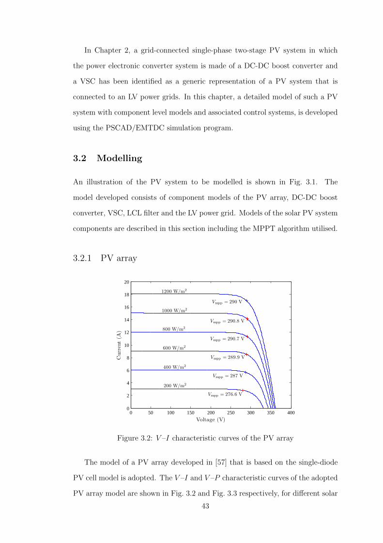
In Chapter 2, a grid-connected single-phase two-stage PV system in which
the power electronic converter system is made of a DC-DC boost converter and
a VSC has been identified as a generic representation of a PV system that is
connected to an LV power grids. In this chapter, a detailed model of such a PV
system with component level models and associated control systems, is developed
using the PSCAD/EMTDC simulation program.
3.2 Modelling
An illustration of the PV system to be modelled is shown in Fig. 3.1. The
model developed consists of component models of the PV array, DC-DC boost
converter, VSC, LCL filter and the LV power grid. Models of the solar PV system
components are described in this section including the MPPT algorithm utilised.
3.2.1 PV array
0 50 100 150 200 250 300 350 4000
2
4
6
8
10
12
14
16
18
20
Vmpp = 290 V
Vmpp = 290.8 V
Vmpp = 290.7 V
Vmpp = 289.9 V
Vmpp = 287 V
Vmpp = 276.6 V
Voltage (V)
Current(A
)
1200 W/m2
1000 W/m2
800 W/m2
600 W/m2
400 W/m2
200 W/m2
Figure 3.2: V –I characteristic curves of the PV array
The model of a PV array developed in [57] that is based on the single-diode
PV cell model is adopted. The V –I and V –P characteristic curves of the adopted
PV array model are shown in Fig. 3.2 and Fig. 3.3 respectively, for different solar
43

0 50 100 150 200 250 300 350 4000
0.5
1.0
1.5
2.0
2.5
3.0
3.5
4.0
4.5
5.0 Pmpp =4.9
Pmpp =4.1
Pmpp =3.3
Pmpp =2.5
Pmpp =1.6
Pmpp =0.8
Voltage / V
Pow
er /
kW
1200 W/m2
800 W/m2
1000 W/m2
600 W/m2
400 W/m2
200 W/m2
Figure 3.3: V -P characteristic curves of the PV array
irradiance levels while the ambient temperature is maintained at 30 C. The
voltage and power levels at the MPP, Vmpp and Pmpp, at each irradiance level are
indicated in Fig. 3.2 and Fig. 3.3 respectively.
3.2.2 MPPT algorithm
The maximum power that can be extracted from a PV array at any given time is
a function of the solar irradiance and the ambient temperature. Since the solar
irradiance and the ambient temperature are changing continuously, an MPPT
algorithm is necessary to track the MPP. In Chapter 2, InC method was identified
as an MPPT algorithm with adequate performance to use in the simulation model
of the PV system. Hence, the InC algorithm is implemented in the developed
simulation model of the PV system.
In the flowchart of Fig. 3.4 that illustrates the InC algorithm, t and (t − 1)
indicate the current sample time and the previous sample time, ∆Vpv and ∆Ipv
represent the difference between two consecutive samples of the output voltage,
Vpv, and current, Ipv, at the PV array output respectively. Vpvref(t) is the voltage
of the tentative MPP that is determined by the InC algorithm at the end of an
iteration and δVpv is the magnitude of voltage that is added/subtracted to/from
44
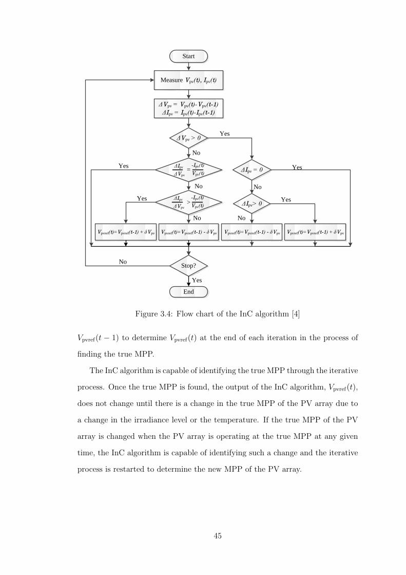
ΔVpv > 0
=
Start
Measure Vpv(t), Ipv(t)
Vpvref(t)=Vpvref(t-1) - δVpv
Stop?
End
ΔVpv = Vpv(t)-Vpv(t-1)ΔIpv = Ipv(t)-Ipv(t-1)
>
ΔIpv = 0
ΔIpv> 0
Vpvref(t)=Vpvref(t-1) - δVpv Vpvref(t)=Vpvref(t-1) + δVpvVpvref(t)=Vpvref(t-1) + δVpv
Yes
No
Yes
Yes
No
NoNo
No
Yes
Yes
No
Yes
ΔVpv
ΔIpv
Vpv(t)-Ipv(t)
ΔVpv
ΔIpv
Vpv(t)-Ipv(t)
Figure 3.4: Flow chart of the InC algorithm [4]
Vpvref(t − 1) to determine Vpvref(t) at the end of each iteration in the process of
finding the true MPP.
The InC algorithm is capable of identifying the true MPP through the iterative
process. Once the true MPP is found, the output of the InC algorithm, Vpvref(t),
does not change until there is a change in the true MPP of the PV array due to
a change in the irradiance level or the temperature. If the true MPP of the PV
array is changed when the PV array is operating at the true MPP at any given
time, the InC algorithm is capable of identifying such a change and the iterative
process is restarted to determine the new MPP of the PV array.
45

3.2.3 Voltage source converter
The VSC in Fig. 3.1 is a full-bridge converter that utilises insulated gate bi-polar
transistor (IGBT) switches. The VSC is able to operate in all four quadrants
provided that necessary control algorithms for such operation are implemented
in the controller of the VSC. The kVA ratting of the VSC, Sr, is 5.4 kVA. The
spare capacity of the VSC when injecting a certain amount of active power is
used for injecting or absorbing reactive power. The switching frequency of the
VSC, fsw, is 25 kHz and a unipolar sinusoidal pulse width modulation technique
is used [58].
3.2.4 LCL filter
The values of the inductors and the capacitor of the LCL filter of the PV sys-
tem shown in Fig. 3.1 were determined as Lfc = 150 µH, Lfg = 75 µH and
Cf = 2.2 µF, by following the design guidelines established in [59]1. Resistances
of inductances Lfc and Lfg are assumed as Rfc = Rfg = 0.001 Ω2. The total induc-
tance of the designed LCL filter is less than 0.1 pu (using a base - Sb = 5.4 kVA,
Vb = 230 V) and the resonant frequency, fres, is 10.7 kHz; less than 0.5fsw. A
damping resistor Rd = 2 Ω, calculated as one third of the impedance of Cf at fres,
is added in series with Cf to improve the stability of the current controller3 [60].
3.2.5 Selection of DC-link capacitor
In a single-phase, grid-connected VSC, the DC-link voltage, Vdc, consists of an
average DC component, Vdcavg, as well as a 100 Hz voltage ripple. The existence of
this 100 Hz voltage ripple in the DC-link voltage of a single-phase grid-connected
1The detailed design procedure of the LCL filter is described in Appendix A.2The damping of the current controller of a PV system is increased if resistance of LCL filter
inductors are high. However, since a higher resistance increases losses, LCL filter inductors aredesigned to have a low resistance.
3The dynamic performance of the current controller with and without the damping resistor,Rd is analysed in Appendix B.
46

VSC is explained in Appendix C. An expression for the peak-to-peak 100 Hz
voltage ripple, ∆Vdc, of the DC-link voltage can be derived as (3.1). The detailed
derivation of (3.1) is given in Appendix C.
In (3.1), Pg is the active power injected to the grid, Cdc is the DC-link capac-
itance and ω is the fundamental angular frequency of the grid voltage, vg.
∆Vdc =Pg
CdcVdcavg ω(3.1)
In the modelled PV system, Cdc is calculated as 2200 µF to limit ∆Vdc to
approximately 5% of Vdcavg when the VSC is injecting 5.4 kW of active power to
the grid and Vdcavg is 400 V.
3.2.6 DC-DC boost converter
The rated capacity of the DC-DC boost converter shown in Fig. 3.1 is 5 kW and
the switching frequency, fdc, is 10 kHz. The current passing through the inductor
Ldc of the DC-DC boost converter consists of a DC component and a switching
ripple. The size of the inductor, Ldc, can be determined using (3.2) [58] in order
to limit the switching frequency associated current ripple, ∆Idc, of the current
that is flowing through the inductor. In (3.2), Vpv is the voltage across the PV
array.
Ldc =Vpv(Vdcavg − Vpv)
∆IdcfdcVdcavg
(3.2)
If the PV array is operated close to the MPP, Vpv is close to 300 V as per
Fig. 3.2 and Fig. 3.3. Hence, the inductor Ldc can be calculated as 9 mH to limit
∆Idc to 5% of the DC current through the inductor Ldc when the DC-DC boost
converter is operating at the rated capacity.
The DC-DC boost converter is able to decouple the PV array from AC-side
dynamics [61]. In modelling the grid-connected PV system, the capacitor Cpv at
the PV array output is chosen to be 2.5 times the DC-link capacitor, Cdc. With
47
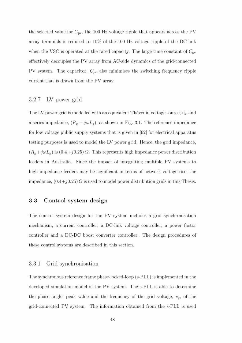
the selected value for Cpv, the 100 Hz voltage ripple that appears across the PV
array terminals is reduced to 10% of the 100 Hz voltage ripple of the DC-link
when the VSC is operated at the rated capacity. The large time constant of Cpv
effectively decouples the PV array from AC-side dynamics of the grid-connected
PV system. The capacitor, Cpv also minimises the switching frequency ripple
current that is drawn from the PV array.
3.2.7 LV power grid
The LV power grid is modelled with an equivalent Thevenin voltage source, vs, and
a series impedance, (Rg + jωLg), as shown in Fig. 3.1. The reference impedance
for low voltage public supply systems that is given in [62] for electrical apparatus
testing purposes is used to model the LV power grid. Hence, the grid impedance,
(Rg +jωLg) is (0.4+j0.25) Ω. This represents high impedance power distribution
feeders in Australia. Since the impact of integrating multiple PV systems to
high impedance feeders may be significant in terms of network voltage rise, the
impedance, (0.4+j0.25) Ω is used to model power distribution grids in this Thesis.
3.3 Control system design
The control system design for the PV system includes a grid synchronisation
mechanism, a current controller, a DC-link voltage controller, a power factor
controller and a DC-DC boost converter controller. The design procedures of
these control systems are described in this section.
3.3.1 Grid synchronisation
The synchronous reference frame phase-locked-loop (s-PLL) is implemented in the
developed simulation model of the PV system. The s-PLL is able to determine
the phase angle, peak value and the frequency of the grid voltage, vg, of the
grid-connected PV system. The information obtained from the s-PLL is used
48
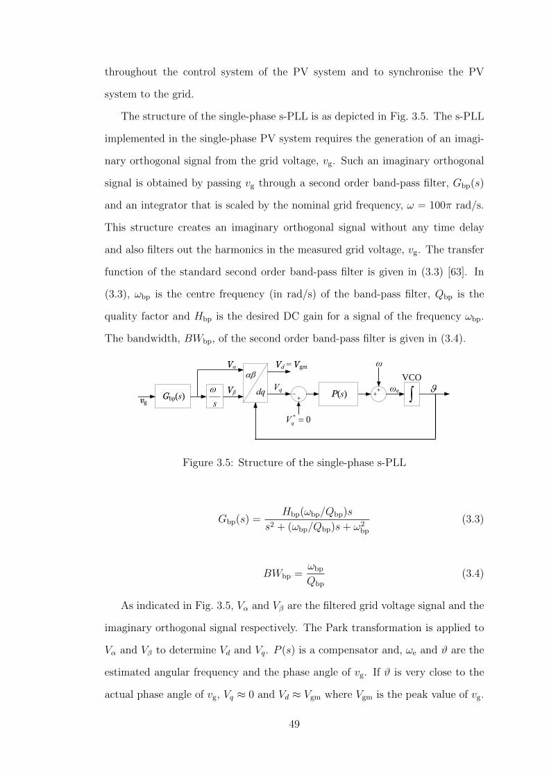
throughout the control system of the PV system and to synchronise the PV
system to the grid.
The structure of the single-phase s-PLL is as depicted in Fig. 3.5. The s-PLL
implemented in the single-phase PV system requires the generation of an imagi-
nary orthogonal signal from the grid voltage, vg. Such an imaginary orthogonal
signal is obtained by passing vg through a second order band-pass filter, Gbp(s)
and an integrator that is scaled by the nominal grid frequency, ω = 100π rad/s.
This structure creates an imaginary orthogonal signal without any time delay
and also filters out the harmonics in the measured grid voltage, vg. The transfer
function of the standard second order band-pass filter is given in (3.3) [63]. In
(3.3), ωbp is the centre frequency (in rad/s) of the band-pass filter, Qbp is the
quality factor and Hbp is the desired DC gain for a signal of the frequency ωbp.
The bandwidth, BWbp, of the second order band-pass filter is given in (3.4).
vgGbp(s)
sω
αβ
dq
0* =qV
P(s) ∫VCO
ϑ
ω
ωe
Vα
Vβ
Vd
Vq
=Vgm
Figure 3.5: Structure of the single-phase s-PLL
Gbp(s) =Hbp(ωbp/Qbp)s
s2 + (ωbp/Qbp)s+ ω2bp
(3.3)
BWbp =ωbp
Qbp
(3.4)
As indicated in Fig. 3.5, Vα and Vβ are the filtered grid voltage signal and the
imaginary orthogonal signal respectively. The Park transformation is applied to
Vα and Vβ to determine Vd and Vq. P (s) is a compensator and, ωe and ϑ are the
estimated angular frequency and the phase angle of vg. If ϑ is very close to the
actual phase angle of vg, Vq ≈ 0 and Vd ≈ Vgm where Vgm is the peak value of vg.
49

The main function of the band-pass filter is to filter out the harmonics in vg.
Therefore, a narrow bandwidth is desired in the band-pass filter so that the low-
order harmonics are well attenuated. Hence a higher Qbp is desired according to
(3.4). But a very low bandwidth slows down the dynamic response of the filter.
Therefore a high value for Qbp cannot be chosen. The chosen value of Qbp is
1.25, so that the BWbp = 40 Hz for a signal of ωbp = 100π rad/s. Since neither
attenuation nor gain is desired for the fundamental frequency grid voltage signal
vg, Hbp = 1. The frequency response and the step response of the designed band-
pass filter are shown in Fig. 3.6 and Fig. 3.7 respectively. As shown in Fig. 3.6,
for a 50 Hz input signal, there is no gain or phase change in the output signal of
the band-pass filter. Based on Fig. 3.7 settling time of the designed band-pass
filter is 30 ms.
−40
−35
−30
−25
−20
−15
−10
−5
0
Mag
nitu
de (
dB)
100
101
102
103
−90
−45
0
45
90
Pha
se (
deg)
Bode Diagram
Frequency (Hz)
Figure 3.6: Frequency response of the band-pass filter
The control loop of the single-phase s-PLL consists only a pole at zero that
is of the voltage-controlled-oscillator (VCO). A PI regulator is chosen as the
compensator P (s). The gains of the PI compensator are selected as kppll = 115
and kipll = 6600. The step response of the closed-loop system is shown in Fig. 3.8
demonstrating a settling time of approximately 70 ms.
50
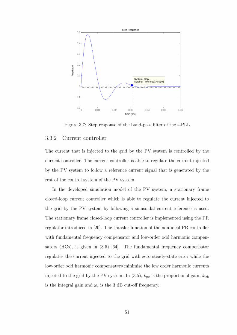
Step Response
Time (sec)
Am
plitu
de
0 0.01 0.02 0.03 0.04 0.05 0.06−0.2
−0.1
0
0.1
0.2
0.3
0.4
0.5
System: GbpSettling Time (sec): 0.0308
Figure 3.7: Step response of the band-pass filter of the s-PLL
3.3.2 Current controller
The current that is injected to the grid by the PV system is controlled by the
current controller. The current controller is able to regulate the current injected
by the PV system to follow a reference current signal that is generated by the
rest of the control system of the PV system.
In the developed simulation model of the PV system, a stationary frame
closed-loop current controller which is able to regulate the current injected to
the grid by the PV system by following a sinusoidal current reference is used.
The stationary frame closed-loop current controller is implemented using the PR
regulator introduced in [20]. The transfer function of the non-ideal PR controller
with fundamental frequency compensator and low-order odd harmonic compen-
sators (HCs), is given in (3.5) [64]. The fundamental frequency compensator
regulates the current injected to the grid with zero steady-state error while the
low-order odd harmonic compensators minimise the low order harmonic currents
injected to the grid by the PV system. In (3.5), kpc is the proportional gain, kich
is the integral gain and ωc is the 3 dB cut-off frequency.
51
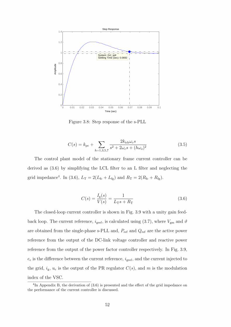
Step Response
Time (sec)
Am
plitu
de
0 0.01 0.02 0.03 0.04 0.05 0.06 0.07 0.08 0.09 0.10
0.2
0.4
0.6
0.8
1
1.2
1.4
System: Gcl_spllSettling Time (sec): 0.0692
Figure 3.8: Step response of the s-PLL
C(s) = kpc +∑
h=1,3,5,7
2kichωcs
s2 + 2ωcs+ (hωo)2(3.5)
The control plant model of the stationary frame current controller can be
derived as (3.6) by simplifying the LCL filter to an L filter and neglecting the
grid impedance4. In (3.6), LT = 2(Lfc + Lfg) and RT = 2(Rfc +Rfg).
C(s) =Ig(s)
V (s)=
1
LTs+RT
(3.6)
The closed-loop current controller is shown in Fig. 3.9 with a unity gain feed-
back loop. The current reference, igref , is calculated using (3.7), where Vgm and ϑ
are obtained from the single-phase s-PLL and, Pref and Qref are the active power
reference from the output of the DC-link voltage controller and reactive power
reference from the output of the power factor controller respectively. In Fig. 3.9,
ec is the difference between the current reference, igref , and the current injected to
the grid, ig, uc is the output of the PR regulator C(s), and m is the modulation
index of the VSC.
4In Appendix B, the derivation of (3.6) is presented and the effect of the grid impedance onthe performance of the current controller is discussed.
52
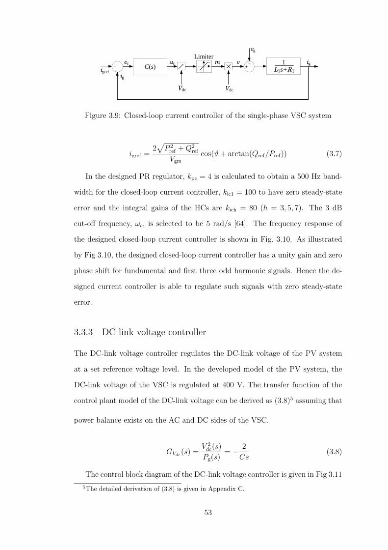
C(s)igigref
1LTs+RTec v
ig
uc
Vdc
Limiter
Vdc
vg
m
Figure 3.9: Closed-loop current controller of the single-phase VSC system
igref =2√P 2
ref +Q2ref
Vgm
cos(ϑ+ arctan(Qref/Pref)) (3.7)
In the designed PR regulator, kpc = 4 is calculated to obtain a 500 Hz band-
width for the closed-loop current controller, kic1 = 100 to have zero steady-state
error and the integral gains of the HCs are kich = 80 (h = 3, 5, 7). The 3 dB
cut-off frequency, ωc, is selected to be 5 rad/s [64]. The frequency response of
the designed closed-loop current controller is shown in Fig. 3.10. As illustrated
by Fig 3.10, the designed closed-loop current controller has a unity gain and zero
phase shift for fundamental and first three odd harmonic signals. Hence the de-
signed current controller is able to regulate such signals with zero steady-state
error.
3.3.3 DC-link voltage controller
The DC-link voltage controller regulates the DC-link voltage of the PV system
at a set reference voltage level. In the developed model of the PV system, the
DC-link voltage of the VSC is regulated at 400 V. The transfer function of the
control plant model of the DC-link voltage can be derived as (3.8)5 assuming that
power balance exists on the AC and DC sides of the VSC.
GVdc(s) =V 2
dc(s)
Pg(s)= − 2
Cs(3.8)
The control block diagram of the DC-link voltage controller is given in Fig 3.11
5The detailed derivation of (3.8) is given in Appendix C.
53
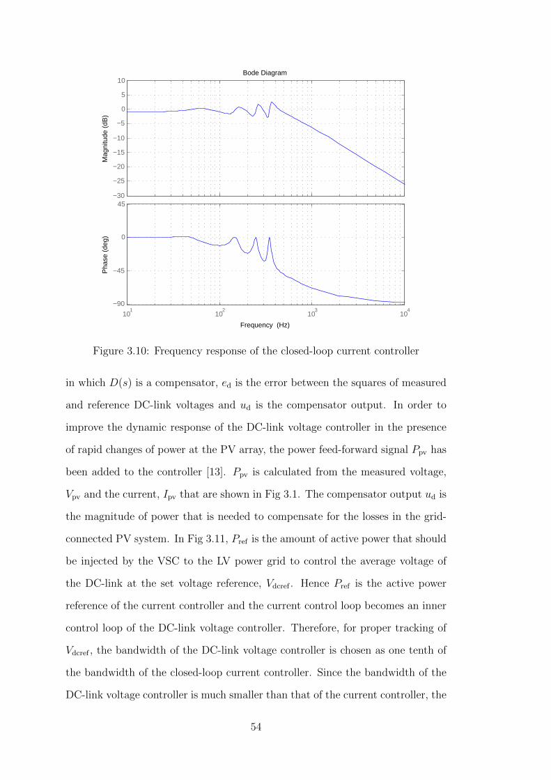
−30
−25
−20
−15
−10
−5
0
5
10
Mag
nitu
de (
dB)
101
102
103
104
−90
−45
0
45
Pha
se (
deg)
Bode Diagram
Frequency (Hz)
Figure 3.10: Frequency response of the closed-loop current controller
in which D(s) is a compensator, ed is the error between the squares of measured
and reference DC-link voltages and ud is the compensator output. In order to
improve the dynamic response of the DC-link voltage controller in the presence
of rapid changes of power at the PV array, the power feed-forward signal Ppv has
been added to the controller [13]. Ppv is calculated from the measured voltage,
Vpv and the current, Ipv that are shown in Fig 3.1. The compensator output ud is
the magnitude of power that is needed to compensate for the losses in the grid-
connected PV system. In Fig 3.11, Pref is the amount of active power that should
be injected by the VSC to the LV power grid to control the average voltage of
the DC-link at the set voltage reference, Vdcref . Hence Pref is the active power
reference of the current controller and the current control loop becomes an inner
control loop of the DC-link voltage controller. Therefore, for proper tracking of
Vdcref , the bandwidth of the DC-link voltage controller is chosen as one tenth of
the bandwidth of the closed-loop current controller. Since the bandwidth of the
DC-link voltage controller is much smaller than that of the current controller, the
54
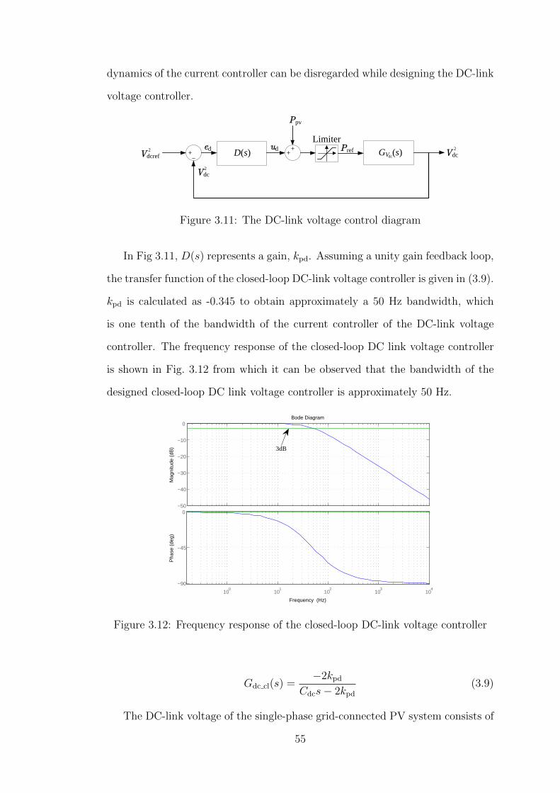
dynamics of the current controller can be disregarded while designing the DC-link
voltage controller.
ed ud
Ppv
D(s)LimiterPref GV (s)dc Vdc
2
Vdc2
Vdcref2
Figure 3.11: The DC-link voltage control diagram
In Fig 3.11, D(s) represents a gain, kpd. Assuming a unity gain feedback loop,
the transfer function of the closed-loop DC-link voltage controller is given in (3.9).
kpd is calculated as -0.345 to obtain approximately a 50 Hz bandwidth, which
is one tenth of the bandwidth of the current controller of the DC-link voltage
controller. The frequency response of the closed-loop DC link voltage controller
is shown in Fig. 3.12 from which it can be observed that the bandwidth of the
designed closed-loop DC link voltage controller is approximately 50 Hz.
−50
−40
−30
−20
−10
0
Mag
nitu
de (
dB)
100
101
102
103
104
−90
−45
0
Pha
se (
deg)
Bode Diagram
Frequency (Hz)
3dB
Figure 3.12: Frequency response of the closed-loop DC-link voltage controller
Gdc cl(s) =−2kpd
Cdcs− 2kpd
(3.9)
The DC-link voltage of the single-phase grid-connected PV system consists of
55
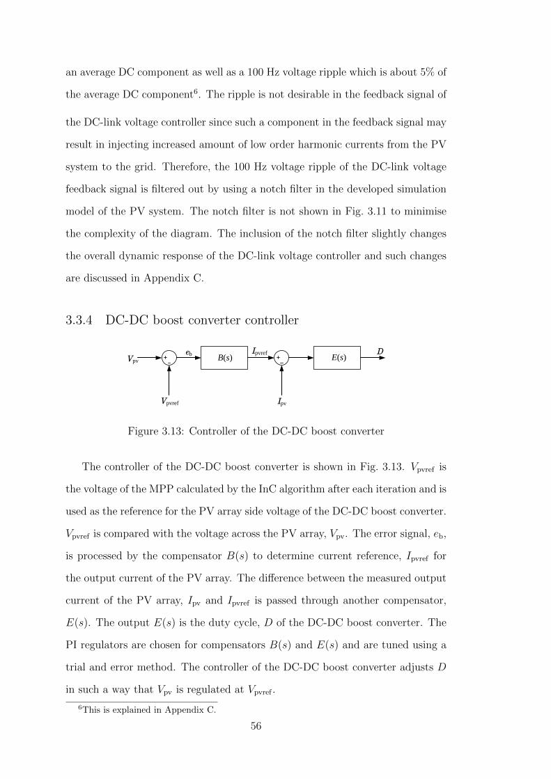
an average DC component as well as a 100 Hz voltage ripple which is about 5% of
the average DC component6. The ripple is not desirable in the feedback signal of
the DC-link voltage controller since such a component in the feedback signal may
result in injecting increased amount of low order harmonic currents from the PV
system to the grid. Therefore, the 100 Hz voltage ripple of the DC-link voltage
feedback signal is filtered out by using a notch filter in the developed simulation
model of the PV system. The notch filter is not shown in Fig. 3.11 to minimise
the complexity of the diagram. The inclusion of the notch filter slightly changes
the overall dynamic response of the DC-link voltage controller and such changes
are discussed in Appendix C.
3.3.4 DC-DC boost converter controller
eb B(s)Ipvref E(s)D
Vpvref
Vpv
Ipv
Figure 3.13: Controller of the DC-DC boost converter
The controller of the DC-DC boost converter is shown in Fig. 3.13. Vpvref is
the voltage of the MPP calculated by the InC algorithm after each iteration and is
used as the reference for the PV array side voltage of the DC-DC boost converter.
Vpvref is compared with the voltage across the PV array, Vpv. The error signal, eb,
is processed by the compensator B(s) to determine current reference, Ipvref for
the output current of the PV array. The difference between the measured output
current of the PV array, Ipv and Ipvref is passed through another compensator,
E(s). The output E(s) is the duty cycle, D of the DC-DC boost converter. The
PI regulators are chosen for compensators B(s) and E(s) and are tuned using a
trial and error method. The controller of the DC-DC boost converter adjusts D
in such a way that Vpv is regulated at Vpvref .
6This is explained in Appendix C.
56
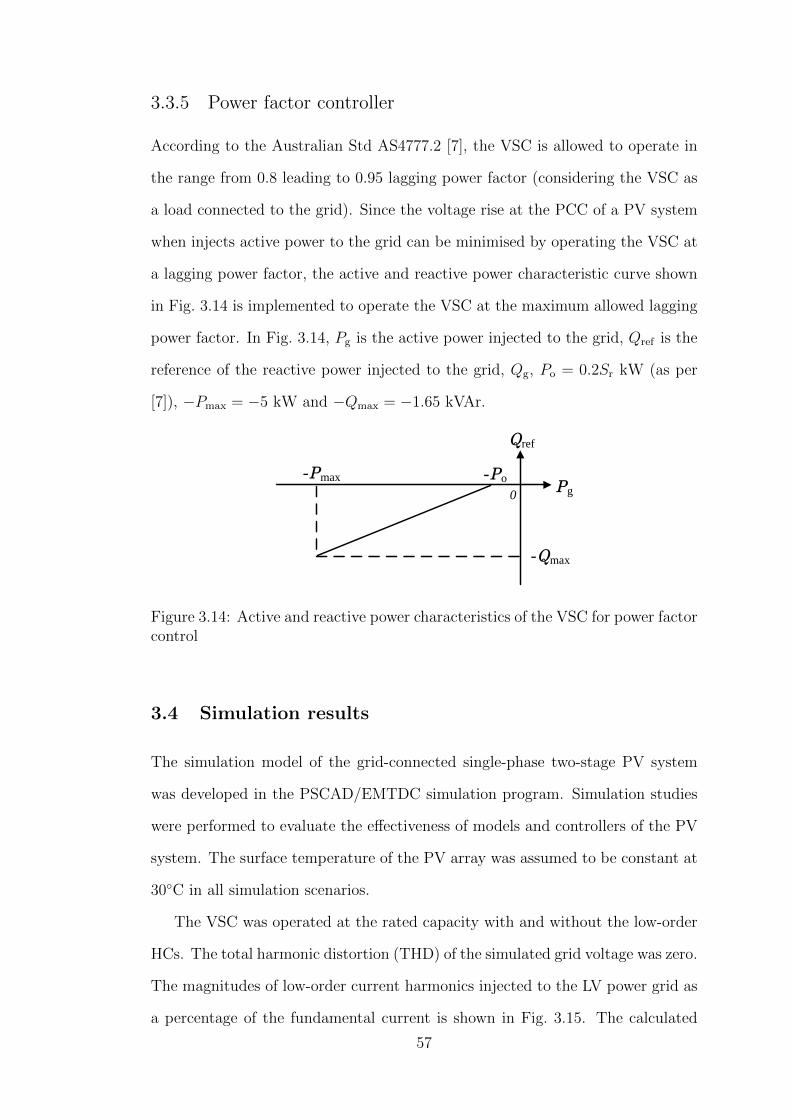
3.3.5 Power factor controller
According to the Australian Std AS4777.2 [7], the VSC is allowed to operate in
the range from 0.8 leading to 0.95 lagging power factor (considering the VSC as
a load connected to the grid). Since the voltage rise at the PCC of a PV system
when injects active power to the grid can be minimised by operating the VSC at
a lagging power factor, the active and reactive power characteristic curve shown
in Fig. 3.14 is implemented to operate the VSC at the maximum allowed lagging
power factor. In Fig. 3.14, Pg is the active power injected to the grid, Qref is the
reference of the reactive power injected to the grid, Qg, Po = 0.2Sr kW (as per
[7]), −Pmax = −5 kW and −Qmax = −1.65 kVAr.
Qref
Pg-Po-Pmax
0
-Qmax
Figure 3.14: Active and reactive power characteristics of the VSC for power factorcontrol
3.4 Simulation results
The simulation model of the grid-connected single-phase two-stage PV system
was developed in the PSCAD/EMTDC simulation program. Simulation studies
were performed to evaluate the effectiveness of models and controllers of the PV
system. The surface temperature of the PV array was assumed to be constant at
30C in all simulation scenarios.
The VSC was operated at the rated capacity with and without the low-order
HCs. The total harmonic distortion (THD) of the simulated grid voltage was zero.
The magnitudes of low-order current harmonics injected to the LV power grid as
a percentage of the fundamental current is shown in Fig. 3.15. The calculated
57
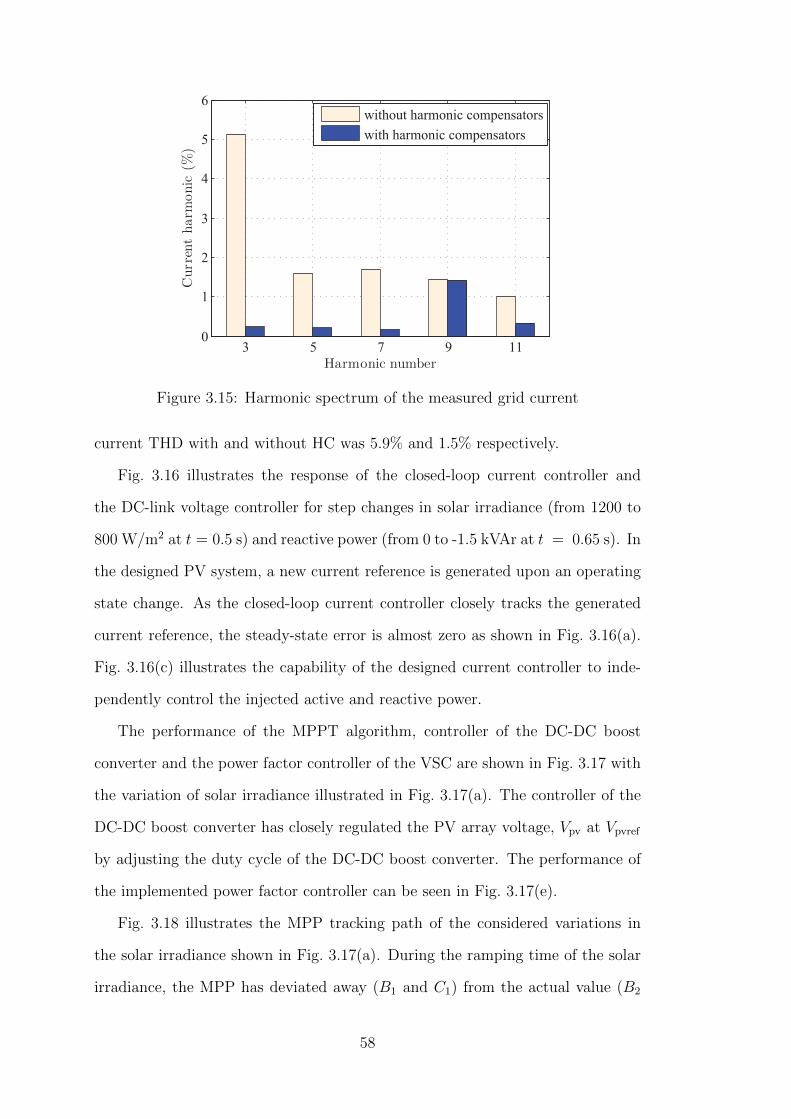
3 5 7 9 110
1
2
3
4
5
6
Harmonic number
Currentharm
onic
(%)
without harmonic compensatorswith harmonic compensators
Figure 3.15: Harmonic spectrum of the measured grid current
current THD with and without HC was 5.9% and 1.5% respectively.
Fig. 3.16 illustrates the response of the closed-loop current controller and
the DC-link voltage controller for step changes in solar irradiance (from 1200 to
800 W/m2 at t = 0.5 s) and reactive power (from 0 to -1.5 kVAr at t = 0.65 s). In
the designed PV system, a new current reference is generated upon an operating
state change. As the closed-loop current controller closely tracks the generated
current reference, the steady-state error is almost zero as shown in Fig. 3.16(a).
Fig. 3.16(c) illustrates the capability of the designed current controller to inde-
pendently control the injected active and reactive power.
The performance of the MPPT algorithm, controller of the DC-DC boost
converter and the power factor controller of the VSC are shown in Fig. 3.17 with
the variation of solar irradiance illustrated in Fig. 3.17(a). The controller of the
DC-DC boost converter has closely regulated the PV array voltage, Vpv at Vpvref
by adjusting the duty cycle of the DC-DC boost converter. The performance of
the implemented power factor controller can be seen in Fig. 3.17(e).
Fig. 3.18 illustrates the MPP tracking path of the considered variations in
the solar irradiance shown in Fig. 3.17(a). During the ramping time of the solar
irradiance, the MPP has deviated away (B1 and C1) from the actual value (B2
58
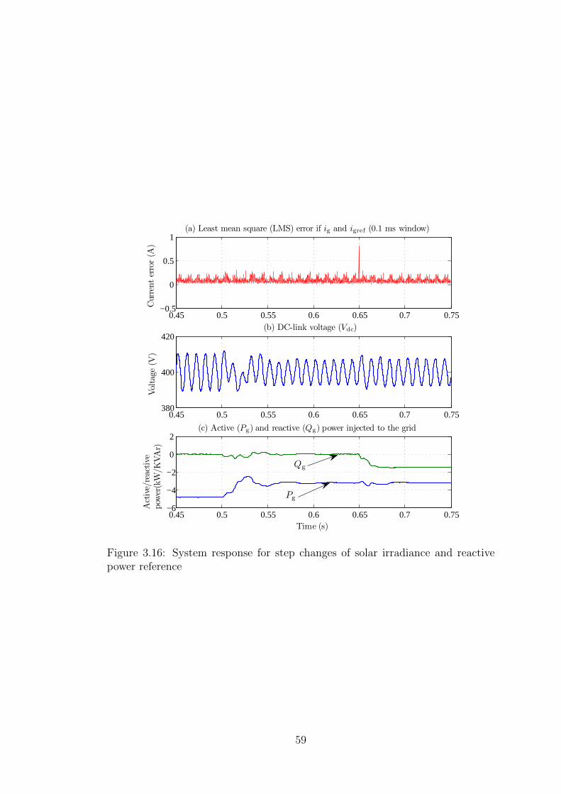
0.45 0.5 0.55 0.6 0.65 0.7 0.75−0.5
0
0.5
1
Currenterror(A
)
(a) Least mean square (LMS) error if ig and igref (0.1 ms window)
0.45 0.5 0.55 0.6 0.65 0.7 0.75−6
−4
−2
0
2(c) Active (Pg) and reactive (Qg) power injected to the grid
Time (s)
Active/reactive
pow
er(kW/K
VAr)
0.45 0.5 0.55 0.6 0.65 0.7 0.75380
400
420(b) DC-link voltage (Vdc)
Voltage
(V)
Pg
Qg
Figure 3.16: System response for step changes of solar irradiance and reactivepower reference
59
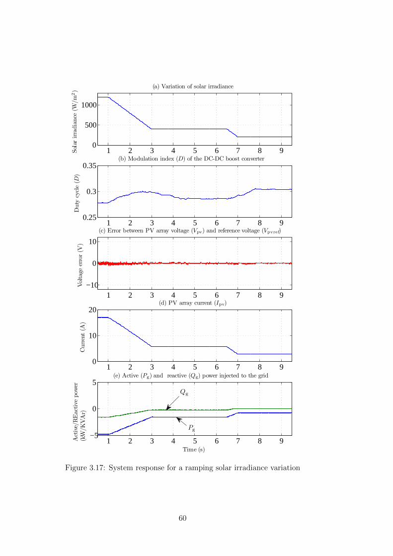
1 2 3 4 5 6 7 8 90
500
1000
Solar
irradiance
(W/m
2)
(a) Variation of solar irradiance
1 2 3 4 5 6 7 8 90.25
0.3
0.35
Duty
cycle(D
)
(b) Modulation index (D) of the DC-DC boost converter
1 2 3 4 5 6 7 8 90
10
20
Current(A
)
(d) PV array current (Ipv)1 2 3 4 5 6 7 8 9
−10
0
10
Voltage
error(V
)
(c) Error between PV array voltage (Vpv) and reference voltage (Vpvref)
1 2 3 4 5 6 7 8 9−5
0
5
Time (s)
Active/REactive
pow
er(kW/K
VAr)
(e) Active (Pg) and reactive (Qg) power injected to the grid
Pg
Qg
Figure 3.17: System response for a ramping solar irradiance variation
60

and C2). However, once the solar irradiance is stabilised, the actual MPP has
been found accurately by the MPPT algorithm.
200 220 240 260 280 300 320 340 3600
2
4
6
8
10
12
14
16
18
20
PV voltage (V)
PV
Curren
t(A
)
200 W/m2
400 W/m2
1200 W/m2
MPP tracking path
B1
C1C2
B2
A
Figure 3.18: MPP tracking path
3.5 Experimental results
An experimental setup using a 5 kW grid-connected single-phase PV system was
established in order to validate the simulation model of the PV system that is
developed in PSCAD/EMTDC simulation program. The control algorithms that
are developed in the simulation model were successfully implemented in the ex-
perimental setup of the PV system. Further details on the experimental setup
including changes that were necessary in the control algorithms and hardware in
the simulation model in order to eliminate practical difficulties when implement-
ing the experimental setup of the PV system are described in Appendix D. The
practical results obtained from the implemented experimental setup of the PV
system are presented in this section. Further, practical results are compared with
the simulation results of the developed simulation model of the PV system that
were presented in Section 3.4 of this chapter, where applicable.
61
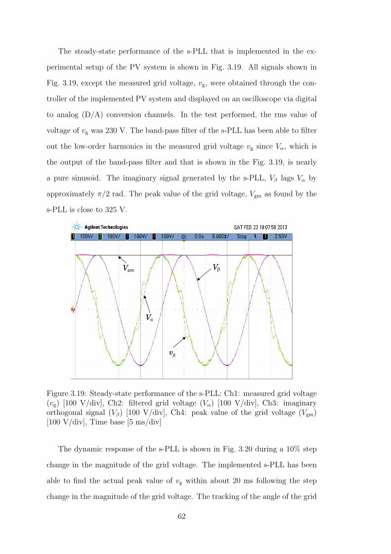
The steady-state performance of the s-PLL that is implemented in the ex-
perimental setup of the PV system is shown in Fig. 3.19. All signals shown in
Fig. 3.19, except the measured grid voltage, vg, were obtained through the con-
troller of the implemented PV system and displayed on an oscilloscope via digital
to analog (D/A) conversion channels. In the test performed, the rms value of
voltage of vg was 230 V. The band-pass filter of the s-PLL has been able to filter
out the low-order harmonics in the measured grid voltage vg since Vα, which is
the output of the band-pass filter and that is shown in the Fig. 3.19, is nearly
a pure sinusoid. The imaginary signal generated by the s-PLL, Vβ lags Vα by
approximately π/2 rad. The peak value of the grid voltage, Vgm as found by the
s-PLL is close to 325 V.
Vgm
Vα
Vβ
vg
Vgm
vg
ϑ
Figure 3.19: Steady-state performance of the s-PLL: Ch1: measured grid voltage(vg) [100 V/div], Ch2: filtered grid voltage (Vα) [100 V/div], Ch3: imaginaryorthogonal signal (Vβ) [100 V/div], Ch4: peak value of the grid voltage (Vgm)[100 V/div], Time base [5 ms/div]
The dynamic response of the s-PLL is shown in Fig. 3.20 during a 10% step
change in the magnitude of the grid voltage. The implemented s-PLL has been
able to find the actual peak value of vg within about 20 ms following the step
change in the magnitude of the grid voltage. The tracking of the angle of the grid
62
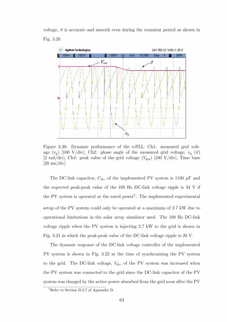
voltage, ϑ is accurate and smooth even during the transient period as shown in
Fig. 3.20.
Vgm
Vα
Vβ
vg
Vgm
vg
ϑ
Figure 3.20: Dynamic performance of the s-PLL: Ch1: measured grid volt-age (vg) [100 V/div], Ch2: phase angle of the measured grid voltage, vg (ϑ)[2 rad/div], Ch4: peak value of the grid voltage (Vgm) [100 V/div], Time base[20 ms/div]
The DC-link capacitor, Cdc, of the implemented PV system is 1100 µF and
the expected peak-peak value of the 100 Hz DC-link voltage ripple is 34 V if
the PV system is operated at the rated power7. The implemented experimental
setup of the PV system could only be operated at a maximum of 2.7 kW due to
operational limitations in the solar array simulator used. The 100 Hz DC-link
voltage ripple when the PV system is injecting 2.7 kW to the grid is shown in
Fig. 3.21 in which the peak-peak value of the DC-link voltage ripple is 20 V.
The dynamic response of the DC-link voltage controller of the implemented
PV system is shown in Fig. 3.22 at the time of synchronising the PV system
to the grid. The DC-link voltage, Vdc, of the PV system was increased when
the PV system was connected to the grid since the DC-link capacitor of the PV
system was charged by the active power absorbed from the grid soon after the PV
7Refer to Section D.2.7 of Appendix D.
63

ΔIpv
ΔVpv
vg
ΔVdc
Figure 3.21: 100 Hz voltage ripple of the DC-link voltage: Ch1: measured gridvoltage (vg) [100 V/div], Ch3: Voltage ripple of the DC-link voltage (∆Vdc)[10 V/div], Time base [2 ms/div]
system was connected to the grid. The DC-link voltage controller has been able
to regulate the DC-link voltage at 420 V within a short period of time (about
20-30 ms) after the PV system was connected to the grid.
The DC-link voltage controller implemented in the PV system has dynamic
characteristics typical of a second-order system as can be seen from the variation
of Vdc in Fig. 3.22. This behaviour is mainly due to the notch filter that is used
to eliminate the 100 Hz voltage ripple of the DC-link voltage feedback signal in
the DC-link voltage controller as discussed in Section 3.3.3 of this chapter.
The waveforms of the current injected to the grid by the PV system, ig, and
the 100 Hz DC-link voltage ripple, ∆Vdc, of the PV system when the PV system
was injecting about 2.3 kW of active power to the grid, is shown in Fig. 3.23.
In this test, the reactive power reference of the PV system was zero. Fig. 3.23
illustrates the capability of the implemented current controller of the PV system
to regulate ig following the reference signal generated by the control system of the
PV system since ig was in phase with vg as shown in Fig. 3.23 when the reactive
power reference is zero.
64
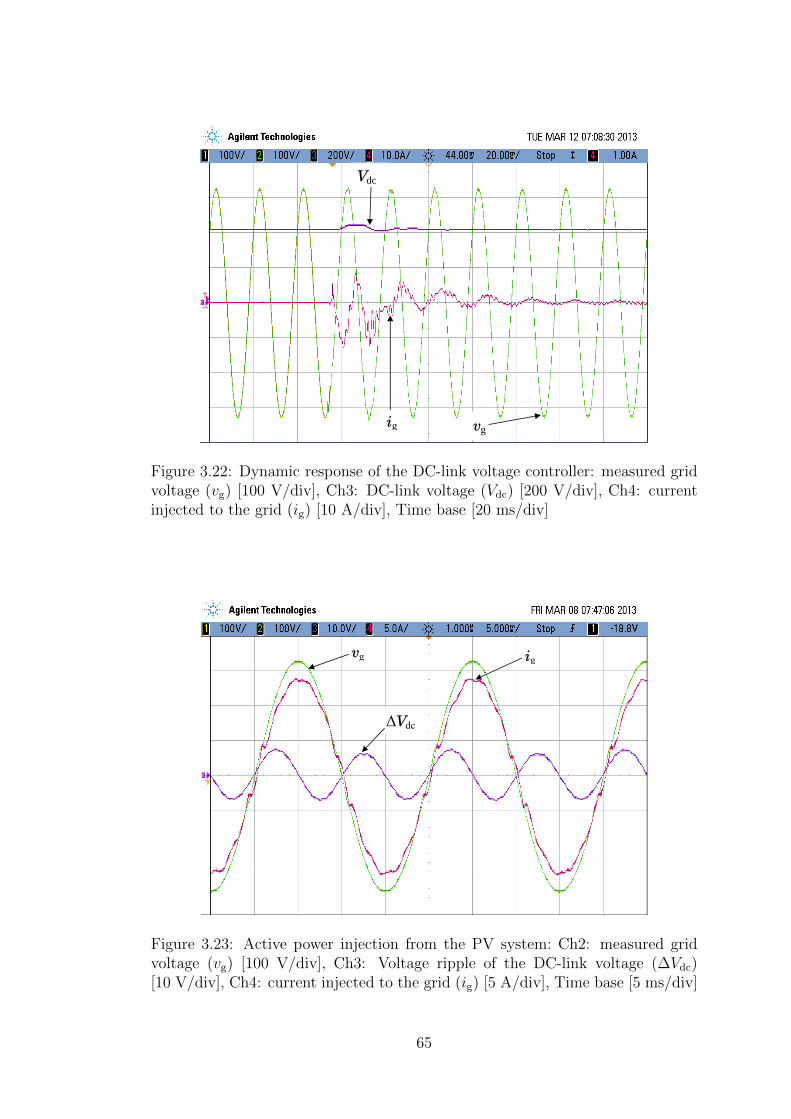
ig
Vdc
vg
vg
ig
Figure 3.22: Dynamic response of the DC-link voltage controller: measured gridvoltage (vg) [100 V/div], Ch3: DC-link voltage (Vdc) [200 V/div], Ch4: currentinjected to the grid (ig) [10 A/div], Time base [20 ms/div]
vg ig
ΔVdc
Ipv Vpv
Figure 3.23: Active power injection from the PV system: Ch2: measured gridvoltage (vg) [100 V/div], Ch3: Voltage ripple of the DC-link voltage (∆Vdc)[10 V/div], Ch4: current injected to the grid (ig) [5 A/div], Time base [5 ms/div]
65

The output voltage of the PV array, Vpv, and the output current of the PV
array, Ipv, during the test performed to obtain Fig. 3.23, is shown in Fig. 3.24.
According to the figures, PV array was injecting about 2.5 kW of active power.
The difference in active power injected to the grid as calculated from Fig. 3.23
and Fig. 3.24 is mainly due to losses in the converter system of the PV system.
vg ig
ΔVdc
Ipv Vpv
Figure 3.24: Outputs of the PV array: Ch3: output voltage of the PV array (Vpv)[100 V/div], Ch4: output current of the PV array (Ipv) [5 A/div], Time base[2 ms/div]
The 100 Hz voltage ripple on the DC-link of the PV system causes a 100 Hz
ripple voltage and current in the output voltage and current of the PV array.
Such voltage and current ripple at the output of the PV system can be minimised
by appropriately tuning the PI regulators in the controller of the DC-DC boost
converter of the PV system.
The voltage ripple, ∆Vpv, and the current ripple, ∆Ipv, at the output of the
PV array during the test performed to obtain Fig. 3.23 and Fig. 3.24 is illustrated
by Fig. 3.25. The high frequency component of ∆Ipv in Fig. 3.25 is the switch-
ing frequency current ripple of the output current of the PV array. According to
Fig. 3.23 and Fig. 3.25, the controller of the DC-DC boost converter of the imple-
mented PV system has been able to limit the peak-peak values of 100 Hz ripple
66
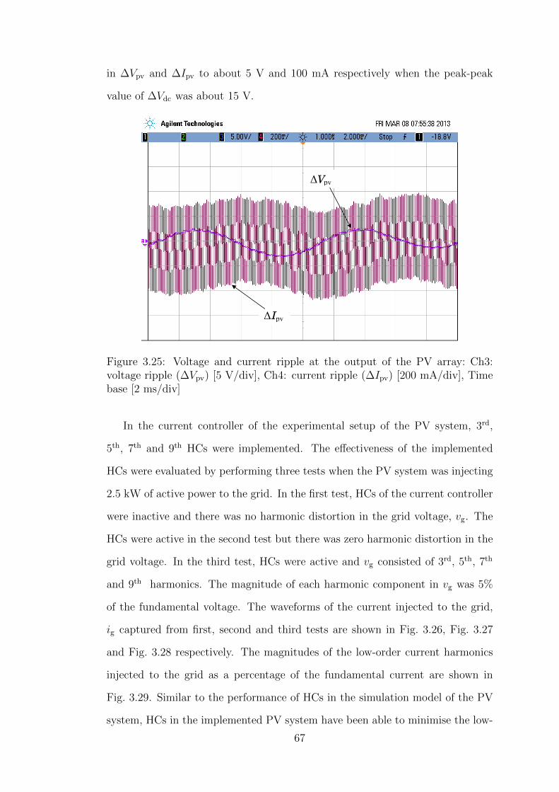
in ∆Vpv and ∆Ipv to about 5 V and 100 mA respectively when the peak-peak
value of ∆Vdc was about 15 V.
ΔIpv
ΔVpv
vg
ΔVdc
Figure 3.25: Voltage and current ripple at the output of the PV array: Ch3:voltage ripple (∆Vpv) [5 V/div], Ch4: current ripple (∆Ipv) [200 mA/div], Timebase [2 ms/div]
In the current controller of the experimental setup of the PV system, 3rd,
5th, 7th and 9th HCs were implemented. The effectiveness of the implemented
HCs were evaluated by performing three tests when the PV system was injecting
2.5 kW of active power to the grid. In the first test, HCs of the current controller
were inactive and there was no harmonic distortion in the grid voltage, vg. The
HCs were active in the second test but there was zero harmonic distortion in the
grid voltage. In the third test, HCs were active and vg consisted of 3rd, 5th, 7th
and 9th harmonics. The magnitude of each harmonic component in vg was 5%
of the fundamental voltage. The waveforms of the current injected to the grid,
ig captured from first, second and third tests are shown in Fig. 3.26, Fig. 3.27
and Fig. 3.28 respectively. The magnitudes of the low-order current harmonics
injected to the grid as a percentage of the fundamental current are shown in
Fig. 3.29. Similar to the performance of HCs in the simulation model of the PV
system, HCs in the implemented PV system have been able to minimise the low-
67

order harmonic current injection to the grid as shown in Fig. 3.29. The calculated
THD of ig in the first test was 8.5%, in the second test was 4.8% and in the third
test was 4.2%.
ig
Vdc
vg
vg
ig
Figure 3.26: Current injected to the grid by the PV system, ig when HCs wereinactive and with zero harmonic distortion in the grid voltage, vg - test 1: Ch1:measured grid voltage (vg) [100 V/div], Ch4: current injected to the grid (ig)[10 A/div], Time base [5 ms/div]
The dynamic behaviour of the DC-link voltage, Vdc, and the current injected
to the grid by the PV system, ig, once the reactive power reference of the PV
system was instantaneously changed from 0 to 2 kVAr is shown in Fig. 3.30. In
Fig. 3.30, ig is in-phase with vg at the beginning since the reactive power reference
at the beginning of the performed test was zero. Once the reactive power reference
was changed to 2 kVAr, ig lags vg since ig was controlled by the current controller
to allow both active and reactive power injection to the grid by the PV system.
The transient in Vdc because of the step change in the reactive power reference
has been stabilised within a short period of time.
The accuracy of operating the PV system at the MPP of the PV array can
be obtained through the user interface of the PV array simulator that is used
in the experimental setup. The variation of the accuracy of the MPP tracking
68

vg
ig
vg
ig
Figure 3.27: Current injected to the grid by the PV system, ig when HCs wereactive and with zero harmonic distortion in the grid voltage, vg - test 2: Ch1:measured grid voltage (vg) [100 V/div], Ch4: current injected to the grid (ig)[10 A/div], Time base [5 ms/div]
vg
ig
vg
ig
Figure 3.28: Current injected to the grid by the PV system, ig when HCswere active and with harmonic distortions in the grid voltage, vg - test 3: Ch1:measured grid voltage (vg) [100 V/div], Ch4: current injected to the grid (ig)[10 A/div], Time base [5 ms/div]
69
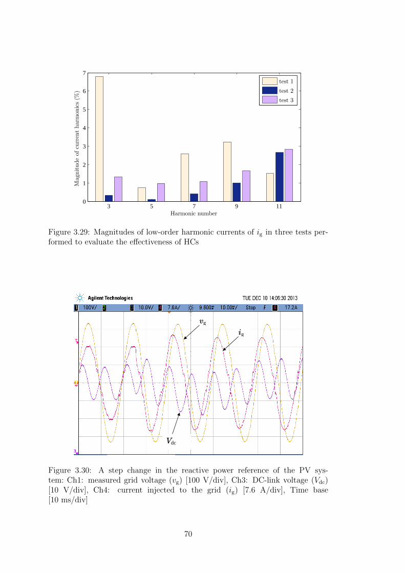
3 5 7 9 110
1
2
3
4
5
6
7
Harmonic number
Mag
nitudeofcu
rren
tharm
onics(%
)
test 1
test 2
test 3
Figure 3.29: Magnitudes of low-order harmonic currents of ig in three tests per-formed to evaluate the effectiveness of HCs
vgig
Vdc
Figure 3.30: A step change in the reactive power reference of the PV sys-tem: Ch1: measured grid voltage (vg) [100 V/div], Ch3: DC-link voltage (Vdc)[10 V/div], Ch4: current injected to the grid (ig) [7.6 A/div], Time base[10 ms/div]
70
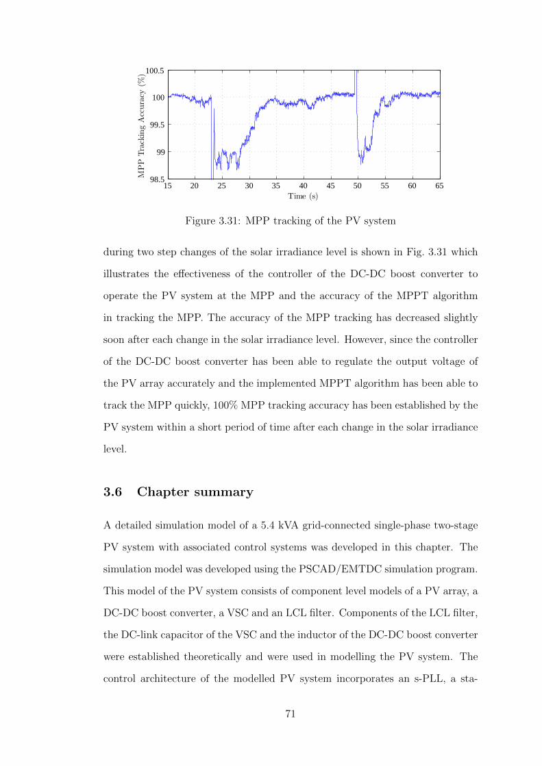
15 20 25 30 35 40 45 50 55 60 6598.5
99
99.5
100
100.5
Time (s)
MPP
TrackingAccuracy
(%)
Figure 3.31: MPP tracking of the PV system
during two step changes of the solar irradiance level is shown in Fig. 3.31 which
illustrates the effectiveness of the controller of the DC-DC boost converter to
operate the PV system at the MPP and the accuracy of the MPPT algorithm
in tracking the MPP. The accuracy of the MPP tracking has decreased slightly
soon after each change in the solar irradiance level. However, since the controller
of the DC-DC boost converter has been able to regulate the output voltage of
the PV array accurately and the implemented MPPT algorithm has been able to
track the MPP quickly, 100% MPP tracking accuracy has been established by the
PV system within a short period of time after each change in the solar irradiance
level.
3.6 Chapter summary
A detailed simulation model of a 5.4 kVA grid-connected single-phase two-stage
PV system with associated control systems was developed in this chapter. The
simulation model was developed using the PSCAD/EMTDC simulation program.
This model of the PV system consists of component level models of a PV array, a
DC-DC boost converter, a VSC and an LCL filter. Components of the LCL filter,
the DC-link capacitor of the VSC and the inductor of the DC-DC boost converter
were established theoretically and were used in modelling the PV system. The
control architecture of the modelled PV system incorporates an s-PLL, a sta-
71

tionary frame current controller, a DC-link voltage controller, a DC-DC boost
converter controller and a MPPT algorithm. The design methodologies that are
followed to establish the control system of the PV system were described in detail.
The effectiveness of the developed model, with theoretically established com-
ponent values and designed controllers was evaluated and verified using simulation
studies. The robustness and the accuracy of the designed grid synchronisation
mechanism, the stationary frame current controller and the DC-link voltage con-
troller were verified by applying rapid changes in solar irradiance and reactive
power reference.
An experimental setup of a PV system that is comparable with the developed
simulation model of the grid-connected single-phase two-stage PV system, was
established to verify the dynamic performance of the developed simulation model
of the PV system. The control system of the PV system that was developed
in the simulation model of the PV system was implemented in the controller of
the experimental setup of the PV system. The experimental results that were
obtained to verify the dynamic performance of the implemented PV system were
presented and discussed. Based on the simulation results of the developed sim-
ulation model of the PV system and the experimental results obtained from the
implemented PV system following conclusions can be made.
• The s-PLL implemented to synchronise the PV system to the grid was
able to determine the phase angle and the peak value of the grid voltage
accurately under steady-state and transient operating conditions of the PV
system. Furthermore, since the s-PLL was implemented with appropriate
low-pass filters, the overall steady-state and dynamic performance of the
s-PLL was seen to be not affected when the grid voltage is distorted.
• The DC-link voltage controller determines the magnitude of the active
power that should be injected/absorbed from/to the grid to regulate the
DC-link voltage at a set reference. The DC-link voltage controller that was
designed has been able to regulate the DC-link voltage at the set reference
72
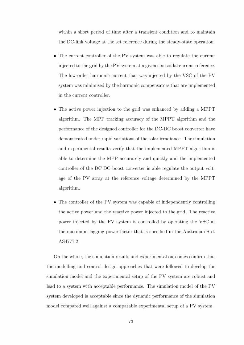
within a short period of time after a transient condition and to maintain
the DC-link voltage at the set reference during the steady-state operation.
• The current controller of the PV system was able to regulate the current
injected to the grid by the PV system at a given sinusoidal current reference.
The low-order harmonic current that was injected by the VSC of the PV
system was minimised by the harmonic compensators that are implemented
in the current controller.
• The active power injection to the grid was enhanced by adding a MPPT
algorithm. The MPP tracking accuracy of the MPPT algorithm and the
performance of the designed controller for the DC-DC boost converter have
demonstrated under rapid variations of the solar irradiance. The simulation
and experimental results verify that the implemented MPPT algorithm is
able to determine the MPP accurately and quickly and the implemented
controller of the DC-DC boost converter is able regulate the output volt-
age of the PV array at the reference voltage determined by the MPPT
algorithm.
• The controller of the PV system was capable of independently controlling
the active power and the reactive power injected to the grid. The reactive
power injected by the PV system is controlled by operating the VSC at
the maximum lagging power factor that is specified in the Australian Std.
AS4777.2.
On the whole, the simulation results and experimental outcomes confirm that
the modelling and control design approaches that were followed to develop the
simulation model and the experimental setup of the PV system are robust and
lead to a system with acceptable performance. The simulation model of the PV
system developed is acceptable since the dynamic performance of the simulation
model compared well against a comparable experimental setup of a PV system.
73

74

Chapter 4
PCC voltage control of a
grid-connected PV system
4.1 Introduction
The integration of multiple PV systems to public LV electricity networks has led
to a grid voltage rise problem as stated in Chapter 2. Since the PCC voltage of a
PV system is sensitive to both active and reactive power injected to the grid by a
PV system, an opportunity exists for PV systems to regulate the respective PCC
voltages by dynamically controlling active and reactive power of the PV system
and help maintaining network voltages within limits. The PCC voltage of a PV
system can be regulated by a closed-loop controller that dynamically controls
the reactive power response of the PV system. Furthermore, in situations where
reactive power capability of a PV system is not adequate to regulate the PCC
voltage, closed-loop active power control is an effective way of regulating PCC
voltage of a PV system as proposed in Chapter 2.
As described in Chapter 2, in the published literature, only limited infor-
mation is available on providing adequate technical details and guidelines for
practically implementing closed-loop controllers that control the active and reac-
tive power response of a PV system in order to regulate the PCC voltage of a PV
system. Therefore, in this Chapter, a detailed design procedure of closed-loop
75

active and reactive power controllers that are capable of dynamically regulating
the PCC voltage of a grid-connected PV system is provided. Plant models of
closed-loop active and reactive power controllers are derived. Further, by com-
bining the operation of closed-loop active and reactive power controllers, two
novel operating strategies are proposed for grid-connected PV systems. Simula-
tion results obtained following the integration of closed-loop active and reactive
power controllers to the simulation model of the PV system that was developed
in Chapter 3 are presented. Experimental results obtained after implementing
novel control systems and operating strategies in the experimental setup of the PV
system1 are provided to demonstrate the robustness of the designed closed-loop
active and reactive power controllers and the feasibility of implementing novel
operating strategies for grid-connected PV systems proposed in this Chapter.
4.2 Simplified model of a distribution feeder
The dynamic active and reactive power controllers proposed in this Chapter are
designed without considering the effects of the dynamic behaviour of loads and
other inverter interfaced energy sources connected to the grid. Hence a simplified
model of a power distribution feeder is considered in the design. The considered
model of the power distribution feeder is shown in Fig. 4.1 where the grid is
modelled with an equivalent Thevenin voltage source (of which the rms voltage at
the terminal is Vs) that is connected in series with a resistor, Rg, and a reactance,
Xg. The rms voltage at the PCC of the PV system is Vg. The term Xf represents
the LCL filter of the PV system. At a given time, the PV system is considered
to inject current Ig to the grid resulting in real power of Pg and reactive power
of Qg. Ig is the rms value of the current injected to the grid by the PV system.
The reference impedance for low voltage public supply systems given in [62]
for electrical apparatus testing purposes is used as the impedance seen by the PV
1Refer to Appendix D for further details on the implemented experimental setup of the PVsystem.
76

Xg
Vs
Power distribution feederPCC
Pg , Qg , IgVg
Xf Rg
PV system
Figure 4.1: Simplified model of a power distribution feeder
system at the PCC when designing dynamic active and reactive power controllers.
Hence the grid impedance of the simplified model of the power distribution feeder
is Rg + jXg = (0.4 + j0.25) Ω. The R/X ratio of the considered grid is approxi-
mately 1.6. As will be shown in Section 4.3, with an R/X ratio greater than unity,
an opportunity exists to regulate the PCC voltage by dynamically controlling the
active and reactive power response of the PV system.
4.3 Decoupling of controllers
An expression for the PCC voltage rise, ∆Vg where ∆Vg = Vg − Vs, when a PV
system is injecting Pg and Qg to the grid, can be derived as given by (4.1)2 using
Fig. 4.1.
∆Vg =−PgRg +QgXg
Vg
(4.1)
The active power injected to the grid by a PV system is controlled by the DC-
link voltage controller as described in Chapter 3. As proposed in this Chapter,
PCC voltage controllers are designed to regulate the PCC voltage by controlling
the active or reactive power injected to the grid by the PV system. According to
(4.1), the PCC voltage, Vg is sensitive to both active and reactive power injected
to the grid by the PV system. As a result, the DC-link voltage controller and PCC
voltage controllers are dynamically coupled. Thus, there should be a decoupling
mechanism for the DC-link voltage controller and PCC voltage controllers of the
2This is derived in 2.6.1
77

PV system to avoid any dynamic interactions between the controllers.
The DC-link voltage controller and PCC voltage controllers can be dynam-
ically decoupled if the grid impedance is measured or estimated [65]. In order
to decouple control systems in this manner, an algorithm to measure or estimate
the grid impedance should be included in the controller design. An alternative
way of decoupling the controllers is to make the response time of one controller
relatively large compared to the response time of the second controller [13]. As a
result of the difference in the response times of controllers, the dynamics are effec-
tively decoupled. A first-order lag element can be utilised to change the response
time of controllers [44]. Alternatively, if the controllers are closed-loop control
systems, the desired response times can be obtained by tuning compensators.
In this Thesis, the tuning of compensators to achieve desired response times is
used in order to decouple controllers. This decoupling technique is commonly
used in control systems of power electronic converters [13]. In order to decouple
two dynamic systems, 2–10 times difference in the response times of the dynamic
systems is adequate [13]. Therefore, in the grid-connected PV system shown in
Fig. 4.1, PCC voltage controllers are made ten times slower than the DC-link
voltage controller in order to decouple the dynamics of these control systems.
4.4 PCC voltage regulation with the dynamic reactive
power controller - (PCC VQ controller)
The design of the closed-loop PCC voltage controller that dynamically controls
the reactive power response of the PV system (herein after referred to as the
PCC VQ controller) is described in detail in this Section.
4.4.1 Control plant model of the PCC VQ controller
In grid-connected PV systems, a phase-locked-loop (PLL) is used to find the phase
angle and the peak value of the PCC voltage. The response time of the PLL is
78
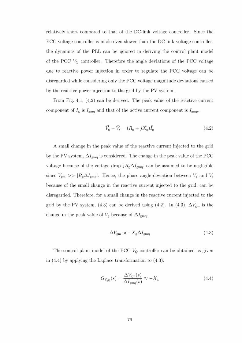
relatively short compared to that of the DC-link voltage controller. Since the
PCC voltage controller is made even slower than the DC-link voltage controller,
the dynamics of the PLL can be ignored in deriving the control plant model
of the PCC VQ controller. Therefore the angle deviations of the PCC voltage
due to reactive power injection in order to regulate the PCC voltage can be
disregarded while considering only the PCC voltage magnitude deviations caused
by the reactive power injection to the grid by the PV system.
From Fig. 4.1, (4.2) can be derived. The peak value of the reactive current
component of Ig is Igmq and that of the active current component is Igmp.
~Vg − ~Vs = (Rg + jXg)~Ig (4.2)
A small change in the peak value of the reactive current injected to the grid
by the PV system, ∆Igmq is considered. The change in the peak value of the PCC
voltage because of the voltage drop jRg∆Igmq, can be assumed to be negligible
since Vgm >> |Rg∆Igmq|. Hence, the phase angle deviation between Vg and Vs
because of the small change in the reactive current injected to the grid, can be
disregarded. Therefore, for a small change in the reactive current injected to the
grid by the PV system, (4.3) can be derived using (4.2). In (4.3), ∆Vgm is the
change in the peak value of Vg because of ∆Igmq.
∆Vgm ≈ −Xg∆Igmq (4.3)
The control plant model of the PCC VQ controller can be obtained as given
in (4.4) by applying the Laplace transformation to (4.3).
GVgQ(s) =∆Vgm(s)
∆Igmq(s)≈ −Xg (4.4)
79
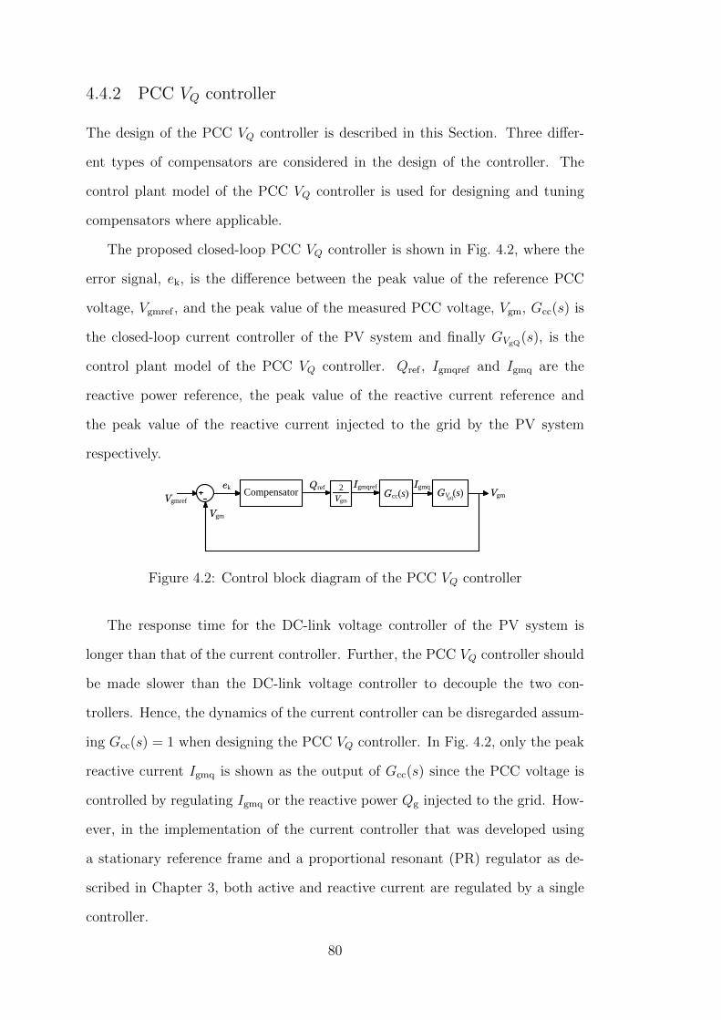
4.4.2 PCC VQ controller
The design of the PCC VQ controller is described in this Section. Three differ-
ent types of compensators are considered in the design of the controller. The
control plant model of the PCC VQ controller is used for designing and tuning
compensators where applicable.
The proposed closed-loop PCC VQ controller is shown in Fig. 4.2, where the
error signal, ek, is the difference between the peak value of the reference PCC
voltage, Vgmref , and the peak value of the measured PCC voltage, Vgm, Gcc(s) is
the closed-loop current controller of the PV system and finally GVgQ(s), is the
control plant model of the PCC VQ controller. Qref , Igmqref and Igmq are the
reactive power reference, the peak value of the reactive current reference and
the peak value of the reactive current injected to the grid by the PV system
respectively.
ekGV (s)
gQVgm
Vgm
VgmrefGcc(s)IgmqQref Igmqref
Vgm
2Compensator
Figure 4.2: Control block diagram of the PCC VQ controller
The response time for the DC-link voltage controller of the PV system is
longer than that of the current controller. Further, the PCC VQ controller should
be made slower than the DC-link voltage controller to decouple the two con-
trollers. Hence, the dynamics of the current controller can be disregarded assum-
ing Gcc(s) = 1 when designing the PCC VQ controller. In Fig. 4.2, only the peak
reactive current Igmq is shown as the output of Gcc(s) since the PCC voltage is
controlled by regulating Igmq or the reactive power Qg injected to the grid. How-
ever, in the implementation of the current controller that was developed using
a stationary reference frame and a proportional resonant (PR) regulator as de-
scribed in Chapter 3, both active and reactive current are regulated by a single
controller.
80
4.4.3 PCC VQ controller - with a proportional gain
A PCC VQ controller with only a proportional gain as the compensator is first
evaluated. The closed-loop transfer function of this controller is a gain since
the plant model of the PCC VQ controller that is given by (4.4) is also a gain.
Therefore, the PCC voltage controller response cannot be made slower than the
DC-link voltage controller of which the closed-loop transfer function is given by
(4.5) as derived in Chapter 3, using only a proportional gain in the control loop.
GVdc cl(s) =
1
0.02s+ 1(4.5)
Furthermore, as there is no integrator in the plant model of the PCC VQ con-
troller derived in (4.4), a zero steady-state error cannot be achieved with only a
proportional gain. Therefore, the PCC VQ controller with a proportional gain as
the compensator, is not suitable for regulating the PCC voltage at a set reference
voltage.
4.4.4 PCC VQ controller - with a proportional gain and a first-order
lag element
In this Section, the PCC VQ controller is evaluated using a combination of a
proportional gain, kpb, and a first-order lag element, Gd(s), as the compensator
in the control loop of the PCC VQ controller. Gd(s) is given by (4.6) where τd is
the time constant.
Gd(s) =1
τds+ 1(4.6)
The closed-loop transfer function of the PCC VQ controller with kpb and Gd(s)
in the control loop is given by (4.7).
GVgQ clpd(s) =2kpbGd(s)GVgQ(s)
Vgm + 2kpbGd(s)GVgQ(s)(4.7)
81
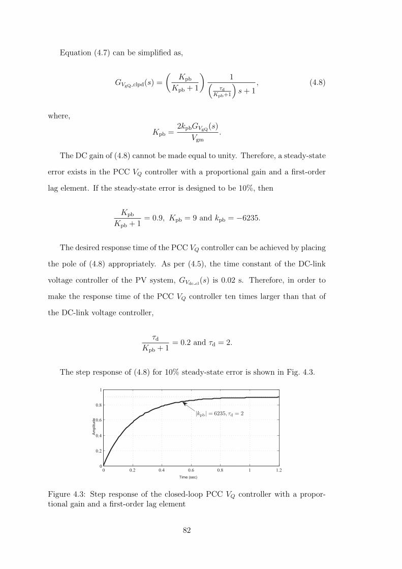
Equation (4.7) can be simplified as,
GVgQ clpd(s) =
(Kpb
Kpb + 1
)1(
τdKpb+1
)s+ 1
, (4.8)
where,
Kpb =2kpbGVgQ(s)
Vgm
.
The DC gain of (4.8) cannot be made equal to unity. Therefore, a steady-state
error exists in the PCC VQ controller with a proportional gain and a first-order
lag element. If the steady-state error is designed to be 10%, then
Kpb
Kpb + 1= 0.9, Kpb = 9 and kpb = −6235.
The desired response time of the PCC VQ controller can be achieved by placing
the pole of (4.8) appropriately. As per (4.5), the time constant of the DC-link
voltage controller of the PV system, GVdc cl(s) is 0.02 s. Therefore, in order to
make the response time of the PCC VQ controller ten times larger than that of
the DC-link voltage controller,
τd
Kpb + 1= 0.2 and τd = 2.
The step response of (4.8) for 10% steady-state error is shown in Fig. 4.3.
0 0.2 0.4 0.6 0.8 1 1.20
0.2
0.4
0.6
0.8
1
Time (sec)
Am
plitu
de
|kpb| = 6235, τd = 2
Figure 4.3: Step response of the closed-loop PCC VQ controller with a propor-tional gain and a first-order lag element
82

The performance of the PCC VQ controller, with a proportional gain and a
first-order lag element was evaluated using the simulation model of the PV system
designed in Chapter 3. The PCC voltage reference was set as Vgmref = 245√
2 V
in the controller. The calculated values for kpb and τd were used in the simulation
study and the results are shown in Fig. 4.4. In the simulation, the PCC voltage
controller was not enabled initially and the rms value of the PCC voltage was set
to approximately 248 V. At time t = 0.5 s, the PCC VQ controller was enabled.
As shown in Fig. 4.4, the designed controller has been able to regulate the PCC
voltage approximately at 245.5 V.
0.4 0.6 0.8 1 1.2 1.4 1.6 1.8 2 2.2245
245.5
246
246.5
247
247.5
248
(a)
Voltage(kV)
PCC voltage (rms) (Vg )
0.4 0.6 0.8 1 1.2 1.4 1.6 1.8 2 2.2−2.5
−2
−1.5
−1
−0.5
0
0.5
(b)Time (s)
Reactivepower
(kVAr)
Reactive power injected to the grid (Qg )
Figure 4.4: Dynamic performance of the PCC VQ controller designed with aproportional gain and a first-order lag element
Fig. 4.4 illustrates that the steady-state value of the PCC voltage has been
reached within approximately 1 s after the PCC VQ controller was enabled. Since
the time constant of (4.8) is 0.2 s, the steady-state PCC voltage has been reached
within five time constants. This observation confirms the accuracy of the plant
model of the PCC VQ controller that is derived in this Chapter.
83
4.4.5 PCC VQ controller - with a proportional gain and an inte-
grator
A zero steady-state error can be achieved by the PCC VQ controller only if the
open-loop transfer function of the controller contains at least one pole that is
closer to the origin. In order to place a pole that is closer to the origin in the
open-loop transfer function of the PCC voltage controller, an integrator with
a scalar can be used as the compensator shown in Fig. 4.2. The closed-loop
transfer function of the PCC voltage controller with a scaled integrator as the
compensator can be derived as,
GVgQ cli(s) =2kpcGVgQ(s)
Vgms+ 2kpcGVgQ(s), (4.9)
where kpc is the scalar of the integrator. Equation (4.9) can be simplified as,
GVgQ cli(s) =1
Kpcs+ 1, (4.10)
where,
Kpc =Vgm
2kpcGVgQ(s).
The pole of GVg cli(s) is selected as one tenth of the pole of GVdc clin (4.5).
Therefore,
Kpc = 0.2 and kpc = −3465.
The pole-zero plot of (4.10) (the pole is labelled as PVg cli) using the reference
grid impedance and when kpc = −3465 is shown in Fig. 4.5. The location of the
pole of the DC-link voltage controller (labelled as PVdc cl) as given by (4.5) is also
shown in Fig. 4.5.
The performance of the PCC VQ controller was evaluated with the simulation
model of the PV system developed in Chapter 3. The PCC voltage reference of the
controller was set as Vgmref = 245√
2 V. Simulation results are shown in Fig. 4.6.
84
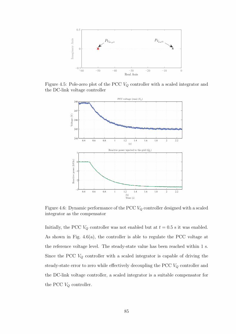
−60 −50 −40 −30 −20 −10 0−0.5
0
0.5
Real AxisIm
aginary
Axis PVg cliPVdc cl
Figure 4.5: Pole-zero plot of the PCC VQ controller with a scaled integrator andthe DC-link voltage controller
0.4 0.6 0.8 1 1.2 1.4 1.6 1.8 2 2.2244
245
246
247
248
(a)
Voltage(V
)
PCC voltage (rms) (Vg )
0.4 0.6 0.8 1 1.2 1.4 1.6 1.8 2 2.2−3
−2
−1
0
1
(b)Time (s)
Reactivepower
(kVAr)
Reactive power injected to the grid (Qg )
Figure 4.6: Dynamic performance of the PCC VQ controller designed with a scaledintegrator as the compensator
Initially, the PCC VQ controller was not enabled but at t = 0.5 s it was enabled.
As shown in Fig. 4.6(a), the controller is able to regulate the PCC voltage at
the reference voltage level. The steady-state value has been reached within 1 s.
Since the PCC VQ controller with a scaled integrator is capable of driving the
steady-state error to zero while effectively decoupling the PCC VQ controller and
the DC-link voltage controller, a scaled integrator is a suitable compensator for
the PCC VQ controller.
85
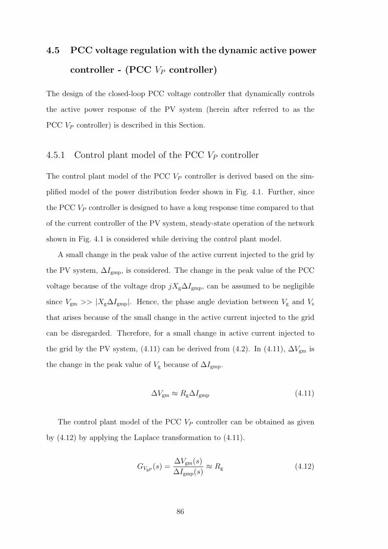
4.5 PCC voltage regulation with the dynamic active power
controller - (PCC VP controller)
The design of the closed-loop PCC voltage controller that dynamically controls
the active power response of the PV system (herein after referred to as the
PCC VP controller) is described in this Section.
4.5.1 Control plant model of the PCC VP controller
The control plant model of the PCC VP controller is derived based on the sim-
plified model of the power distribution feeder shown in Fig. 4.1. Further, since
the PCC VP controller is designed to have a long response time compared to that
of the current controller of the PV system, steady-state operation of the network
shown in Fig. 4.1 is considered while deriving the control plant model.
A small change in the peak value of the active current injected to the grid by
the PV system, ∆Igmp, is considered. The change in the peak value of the PCC
voltage because of the voltage drop jXg∆Igmp, can be assumed to be negligible
since Vgm >> |Xg∆Igmp|. Hence, the phase angle deviation between Vg and Vs
that arises because of the small change in the active current injected to the grid
can be disregarded. Therefore, for a small change in active current injected to
the grid by the PV system, (4.11) can be derived from (4.2). In (4.11), ∆Vgm is
the change in the peak value of Vg because of ∆Igmp.
∆Vgm ≈ Rg∆Igmp (4.11)
The control plant model of the PCC VP controller can be obtained as given
by (4.12) by applying the Laplace transformation to (4.11).
GVgP(s) =∆Vgm(s)
∆Igmp(s)≈ Rg (4.12)
86
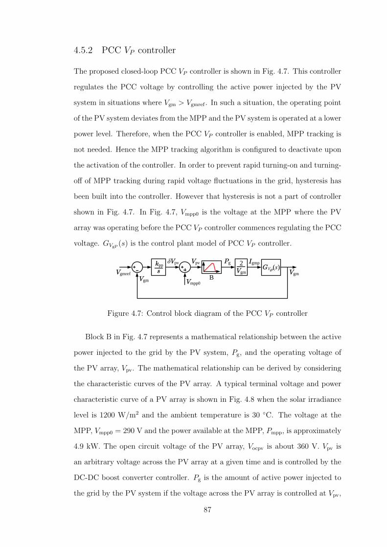
4.5.2 PCC VP controller
The proposed closed-loop PCC VP controller is shown in Fig. 4.7. This controller
regulates the PCC voltage by controlling the active power injected by the PV
system in situations where Vgm > Vgmref . In such a situation, the operating point
of the PV system deviates from the MPP and the PV system is operated at a lower
power level. Therefore, when the PCC VP controller is enabled, MPP tracking is
not needed. Hence the MPP tracking algorithm is configured to deactivate upon
the activation of the controller. In order to prevent rapid turning-on and turning-
off of MPP tracking during rapid voltage fluctuations in the grid, hysteresis has
been built into the controller. However that hysteresis is not a part of controller
shown in Fig. 4.7. In Fig. 4.7, Vmpp0 is the voltage at the MPP where the PV
array was operating before the PCC VP controller commences regulating the PCC
voltage. GVgP(s) is the control plant model of PCC VP controller.
δVpvGV (s)gP VgmVgm
Vgmref
IgmpPg
Vgm
2skpp
BVmpp0
Vpv
Figure 4.7: Control block diagram of the PCC VP controller
Block B in Fig. 4.7 represents a mathematical relationship between the active
power injected to the grid by the PV system, Pg, and the operating voltage of
the PV array, Vpv. The mathematical relationship can be derived by considering
the characteristic curves of the PV array. A typical terminal voltage and power
characteristic curve of a PV array is shown in Fig. 4.8 when the solar irradiance
level is 1200 W/m2 and the ambient temperature is 30 C. The voltage at the
MPP, Vmpp0 = 290 V and the power available at the MPP, Pmpp, is approximately
4.9 kW. The open circuit voltage of the PV array, Vocpv is about 360 V. Vpv is
an arbitrary voltage across the PV array at a given time and is controlled by the
DC-DC boost converter controller. Pg is the amount of active power injected to
the grid by the PV system if the voltage across the PV array is controlled at Vpv,
87
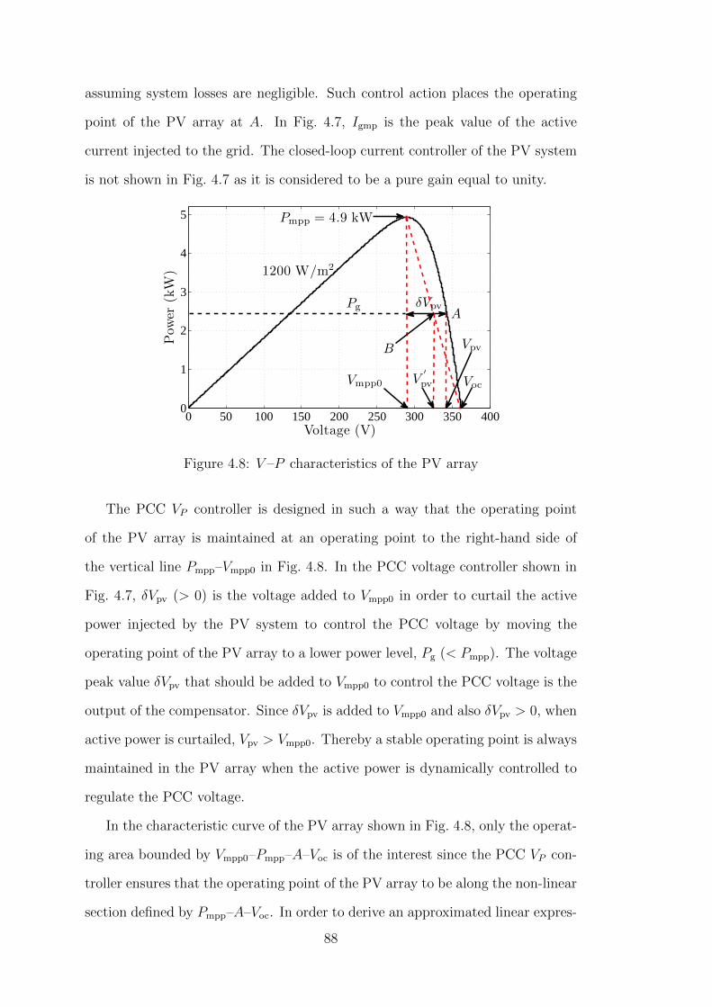
assuming system losses are negligible. Such control action places the operating
point of the PV array at A. In Fig. 4.7, Igmp is the peak value of the active
current injected to the grid. The closed-loop current controller of the PV system
is not shown in Fig. 4.7 as it is considered to be a pure gain equal to unity.
0 50 100 150 200 250 300 350 4000
1
2
3
4
5 Pmpp = 4.9 kW
Voltage (V)
Pow
er(kW
)
δ
1200 W/m2
V′pv
Vpv
Voc
Pg Vpv
Vmpp0
B
A
Figure 4.8: V –P characteristics of the PV array
The PCC VP controller is designed in such a way that the operating point
of the PV array is maintained at an operating point to the right-hand side of
the vertical line Pmpp–Vmpp0 in Fig. 4.8. In the PCC voltage controller shown in
Fig. 4.7, δVpv (> 0) is the voltage added to Vmpp0 in order to curtail the active
power injected by the PV system to control the PCC voltage by moving the
operating point of the PV array to a lower power level, Pg (< Pmpp). The voltage
peak value δVpv that should be added to Vmpp0 to control the PCC voltage is the
output of the compensator. Since δVpv is added to Vmpp0 and also δVpv > 0, when
active power is curtailed, Vpv > Vmpp0. Thereby a stable operating point is always
maintained in the PV array when the active power is dynamically controlled to
regulate the PCC voltage.
In the characteristic curve of the PV array shown in Fig. 4.8, only the operat-
ing area bounded by Vmpp0–Pmpp–A–Voc is of the interest since the PCC VP con-
troller ensures that the operating point of the PV array to be along the non-linear
section defined by Pmpp–A–Voc. In order to derive an approximated linear expres-
88
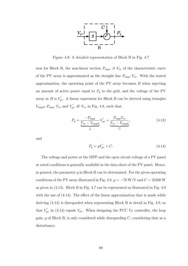
CVpv
B
gPg
Figure 4.9: A detailed representation of Block B in Fig. 4.7
sion for Block B, the non-linear section Pmpp–A–Voc of the characteristic curve
of the PV array is approximated as the straight line Pmpp–Voc. With the stated
approximation, the operating point of the PV array becomes B when injecting
an amount of active power equal to Pg to the grid, and the voltage of the PV
array at B is V′
pv. A linear expression for Block B can be derived using triangles
Vmpp0–Pmpp–Voc and V′
pv–B–Voc in Fig. 4.8, such that,
Pg =−Pmpp
Voc − Vmpp0︸ ︷︷ ︸g
V′
pv +PmppVoc
Voc − Vmpp0︸ ︷︷ ︸C
, (4.13)
and
Pg = gV′
pv + C. (4.14)
The voltage and power at the MPP and the open circuit voltage of a PV panel
at rated conditions is generally available in the data sheet of the PV panel. Hence,
in general, the parameter g in Block B can be determined. For the given operating
conditions of the PV array illustrated in Fig. 4.8, g = −70 W/V and C = 25200 W
as given in (4.14). Block B in Fig. 4.7 can be represented as illustrated in Fig. 4.9
with the use of (4.14). The effect of the linear approximation that is made while
deriving (4.14) is disregarded when representing Block B in detail in Fig. 4.9, so
that V′
pv in (4.14) equals Vpv. When designing the PCC VP controller, the loop
gain, g of Block B, is only considered while disregarding C, considering that as a
disturbance.
89
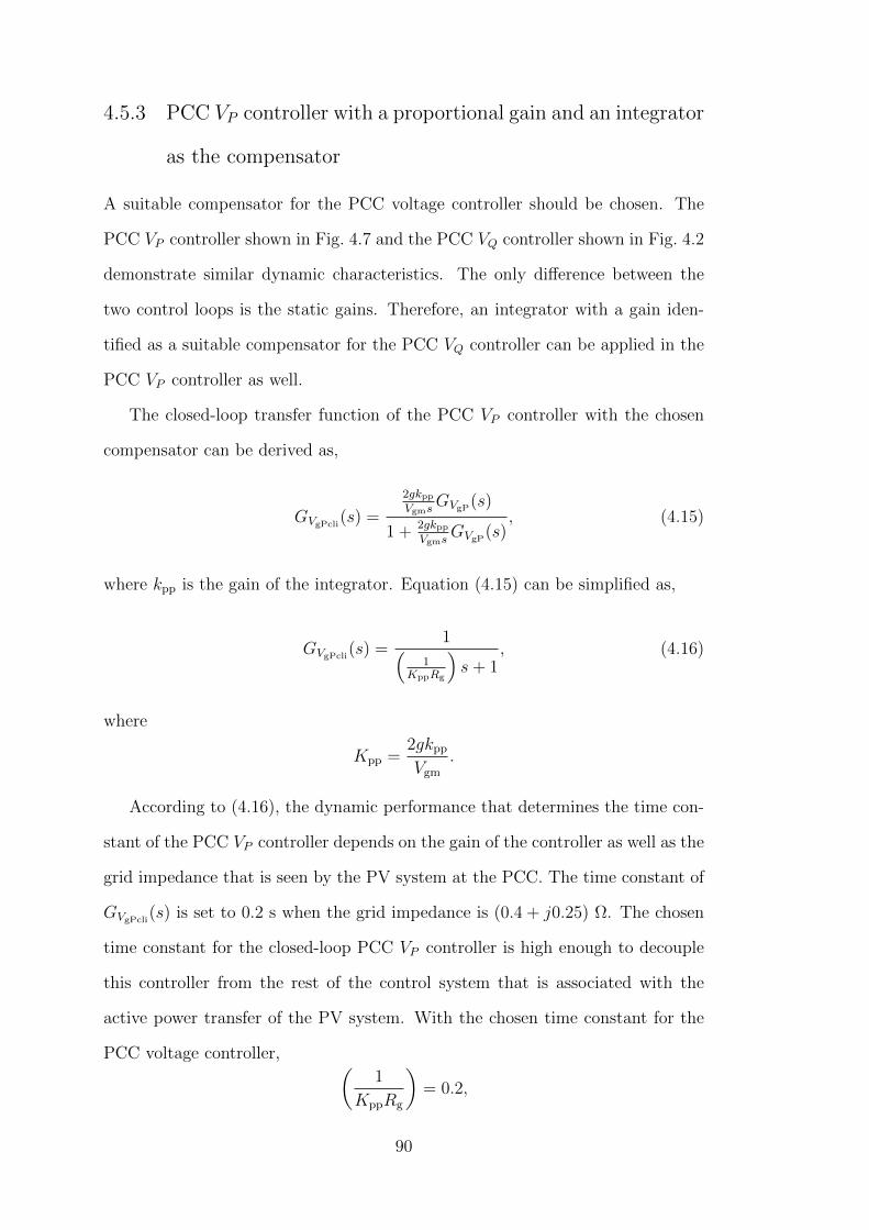
4.5.3 PCC VP controller with a proportional gain and an integrator
as the compensator
A suitable compensator for the PCC voltage controller should be chosen. The
PCC VP controller shown in Fig. 4.7 and the PCC VQ controller shown in Fig. 4.2
demonstrate similar dynamic characteristics. The only difference between the
two control loops is the static gains. Therefore, an integrator with a gain iden-
tified as a suitable compensator for the PCC VQ controller can be applied in the
PCC VP controller as well.
The closed-loop transfer function of the PCC VP controller with the chosen
compensator can be derived as,
GVgPcli(s) =
2gkppVgms
GVgP(s)
1 + 2gkppVgms
GVgP(s), (4.15)
where kpp is the gain of the integrator. Equation (4.15) can be simplified as,
GVgPcli(s) =
1(1
KppRg
)s+ 1
, (4.16)
where
Kpp =2gkpp
Vgm
.
According to (4.16), the dynamic performance that determines the time con-
stant of the PCC VP controller depends on the gain of the controller as well as the
grid impedance that is seen by the PV system at the PCC. The time constant of
GVgPcli(s) is set to 0.2 s when the grid impedance is (0.4 + j0.25) Ω. The chosen
time constant for the closed-loop PCC VP controller is high enough to decouple
this controller from the rest of the control system that is associated with the
active power transfer of the PV system. With the chosen time constant for the
PCC voltage controller, (1
KppRg
)= 0.2,
90
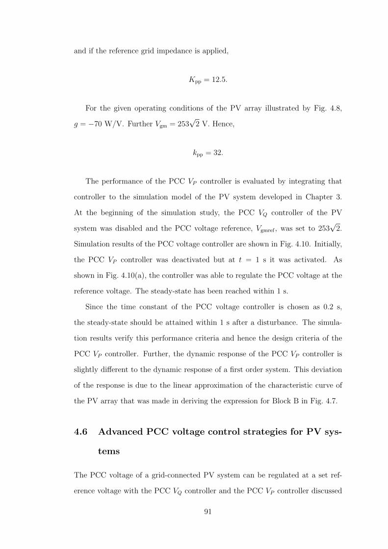
and if the reference grid impedance is applied,
Kpp = 12.5.
For the given operating conditions of the PV array illustrated by Fig. 4.8,
g = −70 W/V. Further Vgm = 253√
2 V. Hence,
kpp = 32.
The performance of the PCC VP controller is evaluated by integrating that
controller to the simulation model of the PV system developed in Chapter 3.
At the beginning of the simulation study, the PCC VQ controller of the PV
system was disabled and the PCC voltage reference, Vgmref , was set to 253√
2.
Simulation results of the PCC voltage controller are shown in Fig. 4.10. Initially,
the PCC VP controller was deactivated but at t = 1 s it was activated. As
shown in Fig. 4.10(a), the controller was able to regulate the PCC voltage at the
reference voltage. The steady-state has been reached within 1 s.
Since the time constant of the PCC voltage controller is chosen as 0.2 s,
the steady-state should be attained within 1 s after a disturbance. The simula-
tion results verify this performance criteria and hence the design criteria of the
PCC VP controller. Further, the dynamic response of the PCC VP controller is
slightly different to the dynamic response of a first order system. This deviation
of the response is due to the linear approximation of the characteristic curve of
the PV array that was made in deriving the expression for Block B in Fig. 4.7.
4.6 Advanced PCC voltage control strategies for PV sys-
tems
The PCC voltage of a grid-connected PV system can be regulated at a set ref-
erence voltage with the PCC VQ controller and the PCC VP controller discussed
91
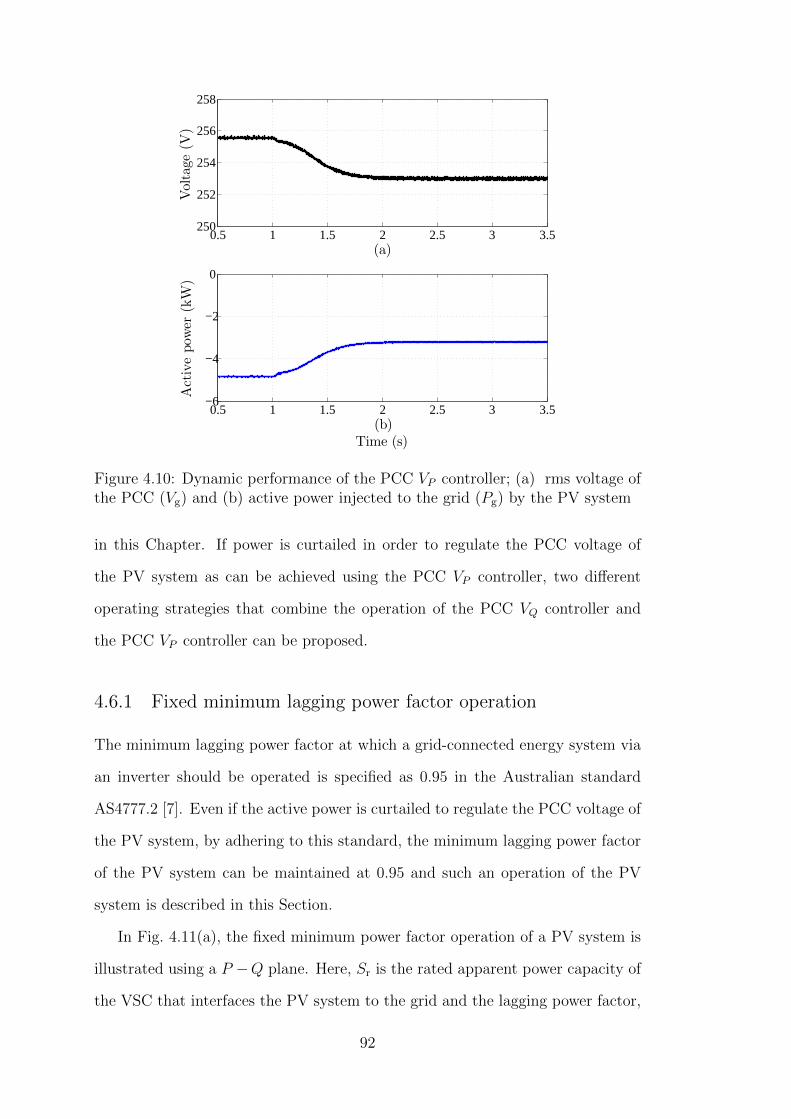
0.5 1 1.5 2 2.5 3 3.5250
252
254
256
258
Voltage
(V)
(a)
0.5 1 1.5 2 2.5 3 3.5−6
−4
−2
0
Activepow
er(kW
)
(b)Time (s)
Figure 4.10: Dynamic performance of the PCC VP controller; (a) rms voltage ofthe PCC (Vg) and (b) active power injected to the grid (Pg) by the PV system
in this Chapter. If power is curtailed in order to regulate the PCC voltage of
the PV system as can be achieved using the PCC VP controller, two different
operating strategies that combine the operation of the PCC VQ controller and
the PCC VP controller can be proposed.
4.6.1 Fixed minimum lagging power factor operation
The minimum lagging power factor at which a grid-connected energy system via
an inverter should be operated is specified as 0.95 in the Australian standard
AS4777.2 [7]. Even if the active power is curtailed to regulate the PCC voltage of
the PV system, by adhering to this standard, the minimum lagging power factor
of the PV system can be maintained at 0.95 and such an operation of the PV
system is described in this Section.
In Fig. 4.11(a), the fixed minimum power factor operation of a PV system is
illustrated using a P −Q plane. Here, Sr is the rated apparent power capacity of
the VSC that interfaces the PV system to the grid and the lagging power factor,
92

Pg/Pn
Qg/Pn
o-1a
b Sr
φ Pg/Pn
Qg/Pn-1
Sr
a
b
c
(a) (b)
Figure 4.11: Advanced operating strategies for a PV system; (a) fixed minimumpower factor operation and (b) fixed maximum apparent power operation
cos(φ) = 0.95. At a given time, the active power injected to the grid by the PV
system is Pg. At the operating point a, the PV system is injecting the nominal
active power, Pn, of the PV system to the grid and hence Pg/Pn = −1. The
PCC VQ controller is active from a to b, and the controller saturates at b as a
result of the PV system reaching the minimum lagging power factor limit. After b,
the MPPT of the PV system is disabled and the PCC VP controller is activated.
The operating point of the PV system moves towards o from b until the PCC
voltage is regulated at the reference voltage. Although the PCC VQ controller
is active from b to o, it does not contribute to dynamic PCC voltage regulation
actively since the controller is saturated.
The operation of the PV system at a minimum lagging power factor is en-
sured by the fixed minimum power factor operation of the PV system. In this
operating mode, the full capacity of the PV system may not be utilised most of
the time. Further, when the PCC VP controller is enabled, in order to maintain
the minimum lagging power factor, the reactive power absorbed from the grid is
reduced in proportion to the amount of active power curtailed. The reduction in
the amount of reactive power absorbed by the PV system causes further active
power curtailment in order to regulate the PCC voltage at the reference level.
93

4.6.2 Fixed maximum apparent power operation
The purpose of defining a minimum power factor in the Australian standard
AS4777.2 [7] is to minimise the reactive power flow in the grid in order to reduce
the network losses and to avoid overloading the distribution transformer in a
large installation of grid-connected energy systems via inverters. The weakest
nodes in an LV grid are the most sensitive nodes to voltage variations and are the
most effective nodes to regulate the voltage. If the reference voltages of dynamic
active and reactive power controllers are properly selected, the PV systems at
weak nodes may start regulating the respective PCC voltage before the other PV
systems in the grid. If the PCC voltage regulation is enabled without limiting
the reactive power absorption to a minimum lagging power factor operation but
limiting to the available capacity of the VSC, the PV systems at the strong nodes
of the grid may not need to contribute to the voltage regulation of the network.
However, the PV systems at weak nodes may contribute to voltage regulation of
the grid utilising their rated capacity. Hence reactive power flow in the network
may be minimised.
The fixed maximum apparent power operation of a PV system is illustrated
in Fig. 4.11(b). The operation of the PV system from a to b is the same as that
was described in Section 4.6.1. At b, the PCC VQ controller is saturated and the
PCC VP controller is activated. Unlike fixed minimum power factor operation,
when power is curtailed to regulate the PCC voltage of the PV system, a pro-
portional amount of reactive power is absorbed by the PV system. Hence, after
b, active power curtailment as well as the additional reactive power absorbed by
the PV system contribute to PCC voltage regulation. Although the PCC VQ con-
troller is enabled after b, it does not contribute to voltage regulation actively since
the controller is saturated.
Since the rated capacity of the VSC that interfaces the PV system to the grid
is used, the active power curtailment to regulate the PCC voltage in the fixed
maximum apparent power operation is less compared to the fixed minimum power
94

factor operation of the PV system. In the fixed minimum power factor operation,
the PV system may disconnect from the grid after curtailing active power up to
a certain level. However, in fixed maximum apparent power operation the PV
system stays connected to the grid even though injecting no active power while
absorbing reactive power to regulate the PCC voltage.
4.7 Experimental results
The dynamic performance of the PCC VQ controller and the PCC VP controller,
and the feasibility of implementing the novel operating strategies proposed for
a PV system in this Chapter, were experimentally verified and the results are
presented and discussed in this Section. The experimental setup of a single-
phase, grid-connected, two-stage PV system established in the laboratory was
used to obtain test results.
A California Instruments MX30 AC and DC power source in combination
with an OMNI 3 − 75 impedance bank was used to simulate the LV grid. The
impedance of the simulated grid was (0.25 + j0.25) Ω3. All experimental results
presented in this Section consists of 4 waveforms; (1) the rms voltage at the PCC
of the PV system, Vg, (2) reactive power injected to the grid, Qg, (3) active power
injected to the grid, Pg, and (4) the current injected to the grid by the PV system,
ig. The first three quantities, Vg, Qg and Pg, were obtained through the controller
and displayed on the oscilloscope via digital to analog (D/A) conversion channels.
The ripple on the waveform of Vg is an artifact of the analog to digital (A/D)
conversion of the measured PCC voltage.
In the controller of the experimental PV system, the voltage reference of
the PCC VQ controller and the PCC VP controller was set as 253√
2 V. The
practical results showing the dynamic performance of the PCC VQ controller and
PCC VP controller and also the proposed novel operating strategies were obtained
3This impedance is different to that is used in simulation studies as specified in Section 4.2.This was because a matching impedance was not available at the time of testing.
95

by introducing a step voltage change in the grid that causes the peak value of the
PCC voltage of the PV system to rise above 253√
2 V.
According to (4.4), the dynamic performance of the PCC VQ controller de-
pends on the reactance, Xg, but not on the resistance, Rg, of the grid impedance
seen by the PV system at the PCC. The reactance values of the grid impedance
as used in the simulation and experimental setup are similar. Hence, the gain of
the integrator as used in the simulation work presented in Section 4.4.5 was used
in the controller of the experimental PV system so that the steady-state of the
PCC VQ controller is reached within 1 s.
Vg
ig
Qg
247.5 V
Vg
ig
Qg
253 V
Pg
Figure 4.12: Performance of the PCC VQ controller: Ch1: rms voltage of the PCC(Vg) [5 V/div] Ch2: reactive power injected to the grid (Qg) [1 kVAr/div], Ch3:active power injected to the grid (Pg) [1 kW/div], Ch4: current injected to thegrid (ig) [10 A/div], Time base [200 ms/div]
The dynamic performance of the PCC VQ controller is shown in Fig. 4.12. The
controller was configured to activate once the peak value of Vg exceeds 253√
2 V.
After the step voltage change in the grid, the PCC voltage is seen to be regulated
at the reference level by absorbing approximately 1.75 kVAr of reactive power
and the steady-state has been reached within approximately 1 s.
Unlike in the case of the PCC VQ controller, the dynamic performance of the
PCC VP controller depends primarily on the resistance of the grid impedance,
Rg, as per (4.12). The resistance of the grid impedance in the simulation work
96

Vg
ig
Qg
253 V
Pg
Figure 4.13: Performance of the PCC VP controller: Ch1: rms voltage of the PCC(Vg) [5 V/div] Ch2: reactive power injected to the grid (Qg) [1 kVAr/div], Ch3:active power injected to the grid (Pg) [1 kW/div], Ch4: current injected to thegrid (ig) [10 A/div], Time base [200 ms/div]
presented in Section 4.5.3 and the experimental PV system are different in mag-
nitude. Therefore the gain of the integrator of the PCC VP controller, kpp is
calculated as 51 to obtain the steady-state response of the PCC VP controller of
the experimental PV system within 1 s, assuming the characteristics of the PV
array are as shown in Fig. 4.8.
Fig. 4.13 illustrates the dynamic performance of the PCC VP controller. After
the step change in voltage of the grid that causes the PCC voltage to rise above
253 V, the controller has been able to regulate the PCC voltage at 253 V by
curtailing approximately 1 kW of active power. The steady-state has been reached
within approximately 1 s. As shown, the smoothness of the Pg variation has been
degraded when Pg is curtailed to regulate the PCC voltage. This behaviour is
introduced by the PV emulator used in the experimental PV system since the PV
emulator is unable to maintain a steady operating point at lower power levels.
The variation of Pg as shown in Fig. 4.13 is comparable with that of Fig. 4.10(b).
The fixed minimum power factor operation and the fixed maximum apparent
power operation of the experimental PV system are illustrated in Fig. 4.14 and
Fig. 4.15 respectively. In the respective operating modes, the minimum power
97
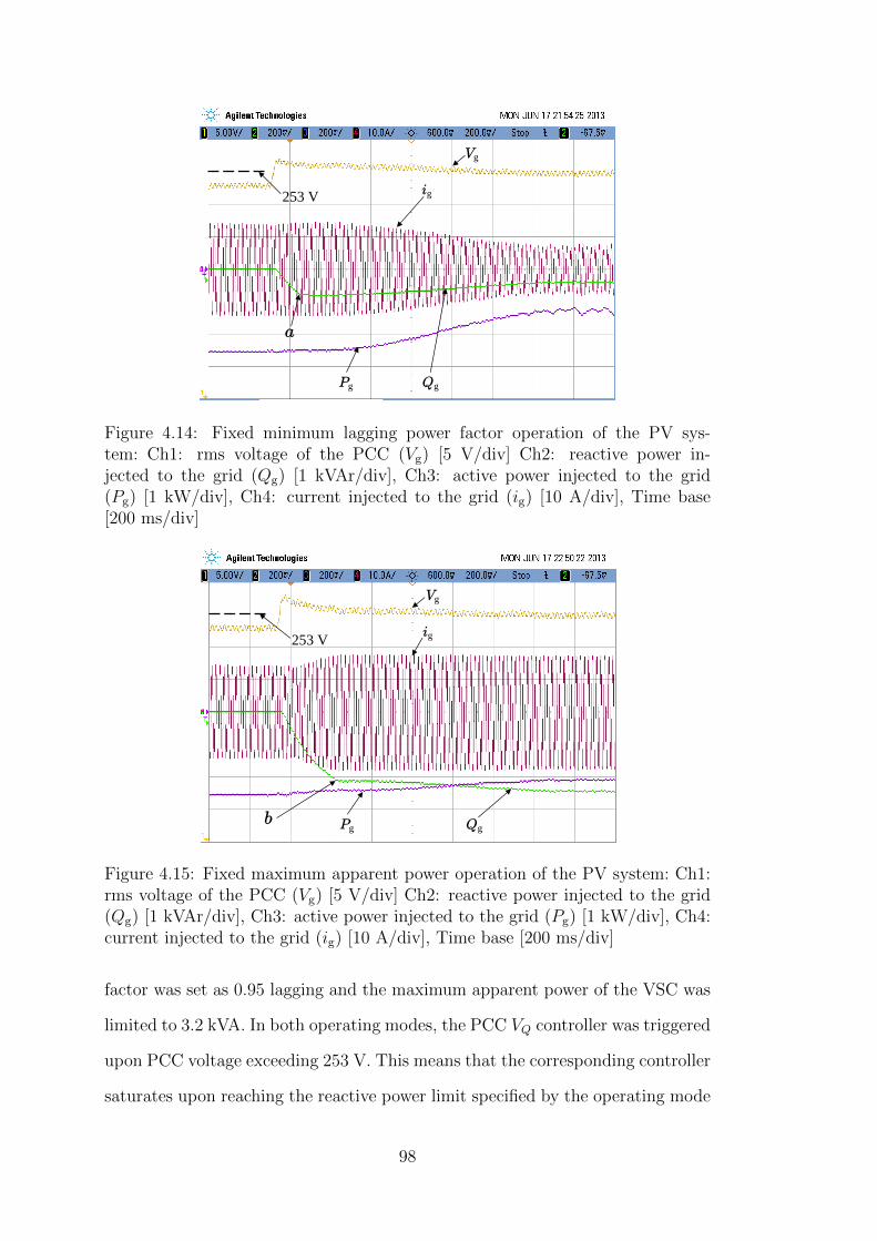
Vg
ig
Qg
253 V
Pg
a
Figure 4.14: Fixed minimum lagging power factor operation of the PV sys-tem: Ch1: rms voltage of the PCC (Vg) [5 V/div] Ch2: reactive power in-jected to the grid (Qg) [1 kVAr/div], Ch3: active power injected to the grid(Pg) [1 kW/div], Ch4: current injected to the grid (ig) [10 A/div], Time base[200 ms/div]
Vg
ig
Qg
253 V
Pg b
Figure 4.15: Fixed maximum apparent power operation of the PV system: Ch1:rms voltage of the PCC (Vg) [5 V/div] Ch2: reactive power injected to the grid(Qg) [1 kVAr/div], Ch3: active power injected to the grid (Pg) [1 kW/div], Ch4:current injected to the grid (ig) [10 A/div], Time base [200 ms/div]
factor was set as 0.95 lagging and the maximum apparent power of the VSC was
limited to 3.2 kVA. In both operating modes, the PCC VQ controller was triggered
upon PCC voltage exceeding 253 V. This means that the corresponding controller
saturates upon reaching the reactive power limit specified by the operating mode
98

at a and b in Fig. 4.14 and Fig. 4.15 respectively. In both operating modes, the
PCC VP controller has been triggered when the PCC VQ controller saturates and
power curtailment commenced in order to regulate the PCC voltage at 253 V. As
illustrated in Fig. 4.15, in the fixed maximum apparent power operation of the
PV system, the PCC voltage can be regulated by curtailing a smaller amount of
active power and obviously absorbing a larger amount of reactive power from the
grid, unlike in the fixed minimum power factor operation of the PV system as
illustrated in Fig. 4.14.
4.8 Chapter summary
In this Chapter, two closed-loop PCC voltage controllers for grid-connected PV
systems were proposed. The proposed PCC VQ controller regulates the PCC volt-
age of a PV system dynamically by controlling the reactive power response of the
PV system and PCC VP controller regulates the PCC voltage of a PV system dy-
namically by controlling the active power response of the PV system. The plant
models of the PCC VQ controller and the PCC VP controller were derived. Three
different compensators were evaluated to identify suitable compensators for the
proposed PCC voltage controllers. Two novel operating strategies, namely fixed
minimum lagging power factor operation and fixed maximum apparent power
operation were proposed. Based on the simulation and experimental results pre-
sented in this Chapter, following conclusions can be drawn.
• The PCC VQ controller and the PCC VP controller proposed in this Chapter
are able to regulate the PCC voltage of a grid-connected PV system at a
given reference voltage with zero steady-state error by controlling the active
or reactive power response of the PV system.
• In order to accurately regulate the PCC voltage at a given reference level,
a suitable compensator should be included in the proposed PCC voltage
controllers. Between the three different compensators that were evaluated,
99

the scaled integrator has been found as the most suitable compensator for
regulating the PCC voltage of the PV system at a given reference voltage
leading to zero steady-state error.
• The derived plant models of The PCC VQ controller and the PCC VP con-
troller are accurate since the dynamics of the designed PCC voltage con-
trollers are predictable. Simulation results and experimental validations
presented in this Chapter prove that the controller design procedures illus-
trated are accurate and robust.
• The fixed minimum power factor operation that was proposed by combining
closed-loop PCC voltage controllers, minimises the reactive power consump-
tion while staying connected to the grid until the power is curtailed to a
specified level. Unlike in the fixed minimum power factor operation, the
maximum apparent power operation proposed in the Chapter may utilise
the full capacity of the VSC that interfaces the PV system to the grid.
Therefore, with the maximum apparent power operation of a PV system,
PCC voltage regulation may be achieved with minimum active power cur-
tailment. Further, the maximum apparent power operation the PV system
may provide voltage support with reactive power even without injecting
any active power to the grid.
• Overall, the closed-loop PCC voltage controllers proposed in this Chapter
will lead to effective and robust PCC voltage regulation of a PV system
employing both active and reactive power. Further, the novel operation
strategies proposed will enable effective utilisation of PV systems in order
to contribute to grid voltage control.
PV systems integrated with dynamic PCC voltage controllers developed in
this Chapter are used to identify interactions between PV systems. The identified
interactions between PV systems are mainly discussed and illustrated in the next
100

chapter, Chapter 5. The key observations discussed in the current chapter form
the basis for most of the analysis presented in Chapter 5.
101

102
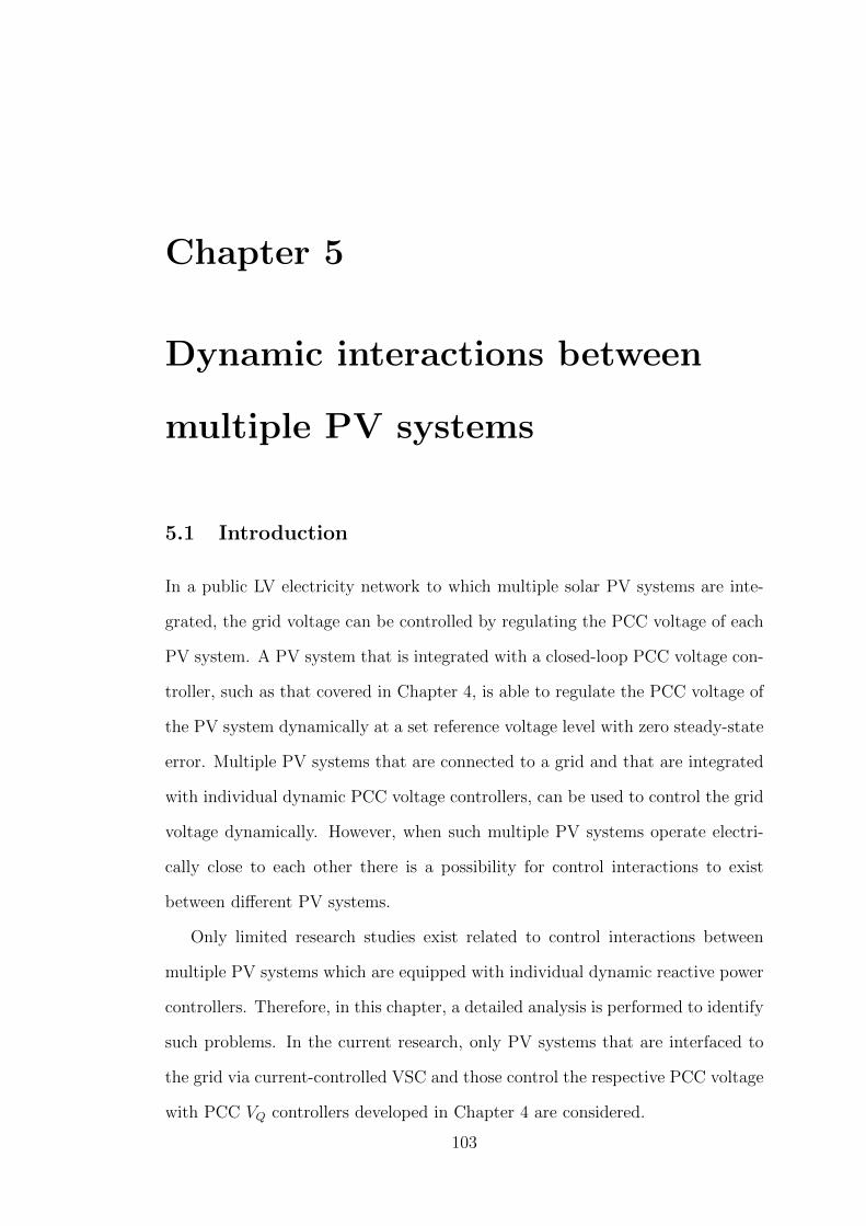
Chapter 5
Dynamic interactions between
multiple PV systems
5.1 Introduction
In a public LV electricity network to which multiple solar PV systems are inte-
grated, the grid voltage can be controlled by regulating the PCC voltage of each
PV system. A PV system that is integrated with a closed-loop PCC voltage con-
troller, such as that covered in Chapter 4, is able to regulate the PCC voltage of
the PV system dynamically at a set reference voltage level with zero steady-state
error. Multiple PV systems that are connected to a grid and that are integrated
with individual dynamic PCC voltage controllers, can be used to control the grid
voltage dynamically. However, when such multiple PV systems operate electri-
cally close to each other there is a possibility for control interactions to exist
between different PV systems.
Only limited research studies exist related to control interactions between
multiple PV systems which are equipped with individual dynamic reactive power
controllers. Therefore, in this chapter, a detailed analysis is performed to identify
such problems. In the current research, only PV systems that are interfaced to
the grid via current-controlled VSC and those control the respective PCC voltage
with PCC VQ controllers developed in Chapter 4 are considered.
103
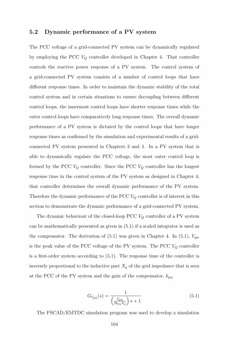
5.2 Dynamic performance of a PV system
The PCC voltage of a grid-connected PV system can be dynamically regulated
by employing the PCC VQ controller developed in Chapter 4. That controller
controls the reactive power response of a PV system. The control system of
a grid-connected PV system consists of a number of control loops that have
different response times. In order to maintain the dynamic stability of the total
control system and in certain situations to ensure decoupling between different
control loops, the innermost control loops have shorter response times while the
outer control loops have comparatively long response times. The overall dynamic
performance of a PV system is dictated by the control loops that have longer
response times as confirmed by the simulation and experimental results of a grid-
connected PV system presented in Chapters 3 and 4. In a PV system that is
able to dynamically regulate the PCC voltage, the most outer control loop is
formed by the PCC VQ controller. Since the PCC VQ controller has the longest
response time in the control system of the PV system as designed in Chapter 4,
that controller determines the overall dynamic performance of the PV system.
Therefore the dynamic performance of the PCC VQ controller is of interest in this
section to demonstrate the dynamic performance of a grid-connected PV system.
The dynamic behaviour of the closed-loop PCC VQ controller of a PV system
can be mathematically presented as given in (5.1) if a scaled integrator is used as
the compensator. The derivation of (5.1) was given in Chapter 4. In (5.1), Vgm
is the peak value of the PCC voltage of the PV system. The PCC VQ controller
is a first-order system according to (5.1). The response time of the controller is
inversely proportional to the inductive part Xg of the grid impedance that is seen
at the PCC of the PV system and the gain of the compensator, kpq.
GVgQ(s) =1(
Vgm2kpqXg
)s+ 1
(5.1)
The PSCAD/EMTDC simulation program was used to develop a simulation
104

Grid
X01R01 N1 N2N0X12R12 N3
PV3
X23R23
Igqm3,Qg3Vg3Vs
Figure 5.1: Network model of a grid-connected PV system
model of the network shown in Fig. 5.1. The simulation model of a PV system
developed in Chapter 3 was integrated to the network as the PV system, PV3.
The PCC VQ controller developed in Chapter 4 was integrated to PV3 and a
scaled integrator was used as the compensator. In Fig. 5.1, Qg3 is the reactive
power absorbed by PV3 and Igmq3 is the peak value of the resulting reactive
current. Vg3 is the rms voltage at the PCC of PV3. The grid impedance at the
PCC of PV3 was (0.28 + j0.27) Ω. With this impedance, the compensator gain
of the PCC VQ controller was set so that steady-state was obtained within 1 s.
Further, the reference voltage of the PCC VQ controller was 253√
2 V and the
controller was configured to operate only if the peak value of the PCC voltage is
greater than the reference voltage level.
Simulation results shown in Fig. 5.2 illustrates the dynamic performance of
the PCC VQ controller of PV3 in the network model shown in Fig. 5.1 after
a step change in the grid voltage, Vs at node N0. As shown in Fig. 5.2, the
PCC VQ controller has been able to regulate the PCC voltage of PV3 at the
reference voltage level nearly within 1 s after the applied step change in the grid
voltage. The dynamic variation shown in Fig. 5.2 is similar to that of the step
response of a first-order system.
105
0.5 1 1.5 2 2.5 3 3.5248
250
252
254
256
Voltage
(V)
(a)
0.5 1 1.5 2 2.5 3 3.5−2
−1.5
−1
−0.5
0
0.5
Reactivepow
er(kVAr)
(b)Time (s)
Figure 5.2: Single PV system operation - dynamic performance of the PCC VQcontroller following a disturbance; (a) rms voltage of the PCC and (b) reactivepower absorbed from the grid (Qg) by the PV system
5.3 Dynamic performance of a PV system in an installa-
tion of multiple PV systems
In a network with multiple PV systems that are operating electrically close to each
other, the dynamic performance of an individual PV system may be different to
that was described in Section 5.2 of this chapter as a result of control interaction
between PV systems. In this section, results of simulation studies performed to
identify possible control interactions between two PV systems that regulate the
respective PCC voltage using PCC VQ controllers are presented.
The dynamic responses of PCC VQ controllers of two PV systems were ob-
tained when these PV systems were connected at the same node. In the simulation
study performed, PV2 and PV3 were connected to node N3 of the network model
shown in Fig. 5.3, at which the grid impedance was (0.28 + j0.27) Ω. The PV
systems were modelled using the detailed simulation model of the PV system
developed in Chapter 3 and the control systems of PV systems, PV2 and PV3
106

Grid
X01R01 N1 N2N0X12R12 N3
PV2
X23R23
Igqm2,Qg2Vg2Vs
PV3
Igqm3,Qg3Vg3
Figure 5.3: Network model of two PV systems connected at the same node
were identical. The PCC VQ controller developed in Chapter 4 was integrated to
both PV2 and PV3 and the gains of PCC VQ controllers in both PV systems were
set to the same value. The reference voltages of PCC VQ controllers were set as
253√
2 V and the controllers were configured to operate only if the peak value of
the PCC voltage is greater than the reference voltage.
0.5 1 1.5 2 2.5 3 3.5248
250
252
254
256
Voltage
(V)
(a)
0.5 1 1.5 2 2.5 3 3.5−2
−1.5
−1
−0.5
0
0.5
Reactivepow
er(kVAr)
(b)Time (s)
Figure 5.4: Operation two PV systems connected at the same node - dynamicperformance of PCC VQ controllers following a disturbance; (a) rms voltage ofthe PCC and (b) reactive power absorbed from the grid (Qg) by the PV system
The simulation results shown in Fig. 5.4 demonstrate the dynamic behaviour
of PCC VQ controllers of PV2 and PV3 when both PV systems were connected
at N3 of the network shown in Fig. 5.3. In this simulation case, the gains of
107
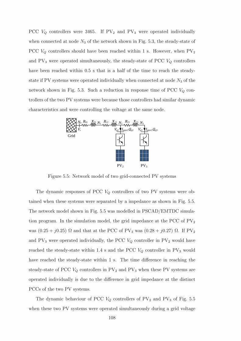
PCC VQ controllers were 3465. If PV2 and PV3 were operated individually
when connected at node N3 of the network shown in Fig. 5.3, the steady-state of
PCC VQ controllers should have been reached within 1 s. However, when PV2
and PV3 were operated simultaneously, the steady-state of PCC VQ controllers
have been reached within 0.5 s that is a half of the time to reach the steady-
state if PV systems were operated individually when connected at node N3 of the
network shown in Fig. 5.3. Such a reduction in response time of PCC VQ con-
trollers of the two PV systems were because those controllers had similar dynamic
characteristics and were controlling the voltage at the same node.
Grid
X01R01 N1 N2N0X12R12 N3
PV2
X23R23
Igqm2,Qg2Vg2Vs
PV3
Igqm3,Qg3Vg3
Figure 5.5: Network model of two grid-connected PV systems
The dynamic responses of PCC VQ controllers of two PV systems were ob-
tained when these systems were separated by a impedance as shown in Fig. 5.5.
The network model shown in Fig. 5.5 was modelled in PSCAD/EMTDC simula-
tion program. In the simulation model, the grid impedance at the PCC of PV2
was (0.25 + j0.25) Ω and that at the PCC of PV3 was (0.28 + j0.27) Ω. If PV2
and PV3 were operated individually, the PCC VQ controller in PV2 would have
reached the steady-state within 1.4 s and the PCC VQ controller in PV3 would
have reached the steady-state within 1 s. The time difference in reaching the
steady-state of PCC VQ controllers in PV2 and PV3 when these PV systems are
operated individually is due to the difference in grid impedance at the distinct
PCCs of the two PV systems.
The dynamic behaviour of PCC VQ controllers of PV2 and PV3 of Fig. 5.5
when these two PV systems were operated simultaneously during a grid voltage
108

5 10 15 20 25 30
250
255
260
(a)Voltage(V
)
5 10 15 20 25 30−8
−6
−4
−2
0
(b)Time (s)
Rea
ctiv
e po
wer
(kV
Ar)
PV3
PV2
PV2
PV3
Figure 5.6: Operation of multiple PV systems - dynamic performance of PCC VQcontrollers following a disturbance; (a) rms voltage of the PCC and (b) reactivepower absorbed from the grid (Qg) by the PV system
disturbance is shown in Fig. 5.6. The figure illustrates that the steady-state of
both controllers was reached within 25-30 s following the grid disturbance. The
time taken by PCC VQ controllers of the two PV systems to reach the steady-state
when two PV systems were operated simultaneously was larger than was expected
if these PV systems were operated individually. Fig. 5.2(b) and Fig. 5.6(b) clearly
illustrates that when two PV systems are operated electrically close to each other,
the dynamic behaviour of the PCC VQ controller of one PV system is affected by
the operation of the PCC VQ controller of the other PV system because of dynamic
interactions between PV systems. The dynamic response shown in Fig. 5.6(b) of
the PV system is similar to the dynamic behaviour of a first-order system which
has a considerably long response time.
Simulation studies were carried out further to identify the impact of set val-
ues of reference voltages of PCC VQ controllers on the dynamic performance of
PCC VQ controllers of PV2 and PV3 in the network model shown in Fig. 5.5. The
simulation results obtained after setting two different reference voltages have con-
109
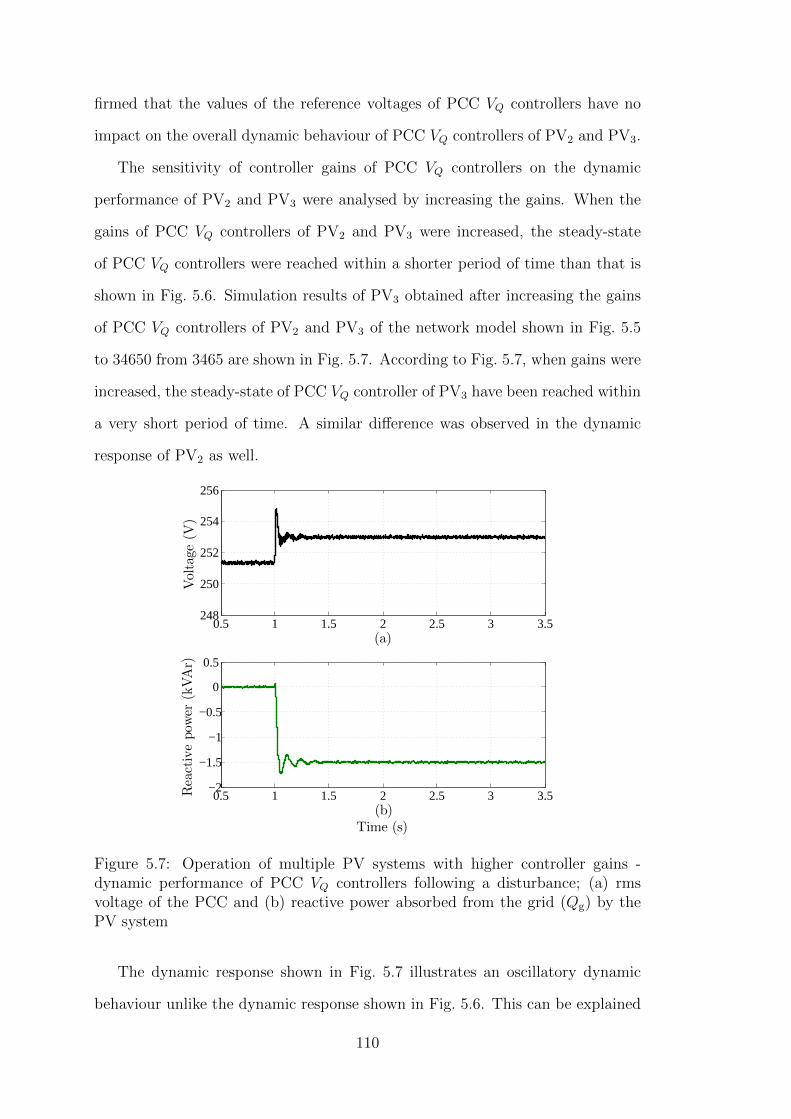
firmed that the values of the reference voltages of PCC VQ controllers have no
impact on the overall dynamic behaviour of PCC VQ controllers of PV2 and PV3.
The sensitivity of controller gains of PCC VQ controllers on the dynamic
performance of PV2 and PV3 were analysed by increasing the gains. When the
gains of PCC VQ controllers of PV2 and PV3 were increased, the steady-state
of PCC VQ controllers were reached within a shorter period of time than that is
shown in Fig. 5.6. Simulation results of PV3 obtained after increasing the gains
of PCC VQ controllers of PV2 and PV3 of the network model shown in Fig. 5.5
to 34650 from 3465 are shown in Fig. 5.7. According to Fig. 5.7, when gains were
increased, the steady-state of PCC VQ controller of PV3 have been reached within
a very short period of time. A similar difference was observed in the dynamic
response of PV2 as well.
0.5 1 1.5 2 2.5 3 3.5248
250
252
254
256
Voltage
(V)
(a)
0.5 1 1.5 2 2.5 3 3.5−2
−1.5
−1
−0.5
0
0.5
Reactivepow
er(kVAr)
(b)Time (s)
Figure 5.7: Operation of multiple PV systems with higher controller gains -dynamic performance of PCC VQ controllers following a disturbance; (a) rmsvoltage of the PCC and (b) reactive power absorbed from the grid (Qg) by thePV system
The dynamic response shown in Fig. 5.7 illustrates an oscillatory dynamic
behaviour unlike the dynamic response shown in Fig. 5.6. This can be explained
110
as follows. The PCC VQ controller is the most outer control layer of a PV system.
Hence, the PCC VQ controller is designed to have a longer response time in order
to decouple the dynamics of that controller from the rest of the control system of
the PV system. The required response time of the PCC VQ controller is obtained
by selecting a suitable gain for the compensator of the controller. When the gain
of the PCC VQ controller of a PV system is 3465 and the grid impedance at the
PCC of the PV system is (0.28 + j0.27) Ω, the steady-state of the PCC VQ con-
troller is reached within 1 s. The response time of 1 s in the PCC VQ controller
is adequate to decouple this controller from the rest of the control system of the
PV system as shown in Chapter 4. When the gain of the PCC VQ controller is
increased from 3465 to 34650, the response time of the controller becomes very
short. Further, dynamic decoupling between the PCC VQ controller and the rest
of the control system has been degraded resulting oscillatory dynamics as shown
in Fig. 5.7. Therefore, though the dynamic interactions between PV systems
demonstrated in Fig. 5.6 can be minimised by increasing gains of PCC VQ con-
trollers that is not the most suitable method to use.
Droop control is widely used in control systems for electrical machines and
power electronic drives. Such a controller is able to extend the operating range of
a power converter system that the controller is built into, improve the dynamic
stability when multiple converter systems are operated electrically close to each
other and to enforce automatic load sharing [14][66]. Therefore a droop controller
was integrated to the PCC VQ controller and control interactions between multiple
PV systems were investigated.
The network model shown in Fig. 5.5 was used to investigate control in-
teractions between PV systems when droop controllers are integrated to the
PCC VQ controllers of PV2 and PV3. The droop controller shown in Fig. 5.8
was integrated to the PCC VQ controller of PV2 and PV3. In Fig. 5.8, Qg is the
reactive power injected by a PV system to the grid. The simulation results of
PV2 and PV3 obtained during a grid voltage disturbance are shown in Fig. 5.9.
111

ekGV (s)
gQ
Vgm
Vgm
VgmrefGcc(s)IgmqQref Igmqref
Vgm
2skpq
kdr
Qg
Droop characteristics
Figure 5.8: Control block diagram of the PCC VQ controller integrated with adroop controller
According to Fig. 5.9, the PCC VQ controllers of PV2 and PV3 have reached the
steady-state within 1 s when droop controllers were integrated. When dynamic
variations of Qg in Fig. 5.6 and Fig. 5.9 are compared, the droop controller has
been able to minimise the effect of control interactions between PV systems and
improve the reactive power sharing between PV systems.
1 2 3 4 5 6 7 8 9 10
250
255
260
Voltage(V
)
(a)
1 2 3 4 5 6 7 8 9 10
−4
−2
0
Reactivepower
(kVAr)
(b)Time (s)
PV3
PV2
PV2
PV3
Figure 5.9: Operation of two PV systems integrated with droop control in PCC VQcontrollers - dynamic performance of PCC VQ controllers following a disturbance;(a) rms voltage of the PCC and (b) reactive power absorbed from the grid (Qg)by the PV system
The impact of the number of PV systems connected to a grid on the dynamic
behaviour of PV systems were investigated by increasing the number of PV sys-
112

Grid
X01R01 N1 N2N0X12R12 N3
PV2
X23R23
Igqm2,Qg2Vg2Vs
PV3
Igqm3,Qg3Vg3
PV1
Igqm1,Qg1Vg1
Figure 5.10: Network model of three grid-connected PV systems
5 10 15 20 25 30
250
255
260
(a)
Voltage(V
)
5 10 15 20 25 30−8
−6
−4
−2
0
(b)Time (s)
Rea
ctiv
e po
wer
(kV
Ar)
PV1
PV2
PV3
PV1 PV2
PV3
Figure 5.11: Operation of three PV systems - dynamic performance of PCC VQcontrollers following a disturbance; (a) rms voltage of the PCC and (b) reactivepower absorbed from the grid (Qg) by the PV system.
tems connected to the network model shown in Fig. 5.5. The network model
shown in Fig. 5.10 was used to investigate the dynamic behaviour of PV systems
when three PV systems are operated simultaneously. The dynamic behaviour of
PCC VQ controllers when all three PV systems, PV1, PV2 and PV3, were oper-
ated simultaneously are shown in Fig. 5.11. According to the results shown, all
three PV systems have attempted to regulate respective PCC voltage by absorb-
ing reactive power from the grid followed by the disturbance. After about 2 s,
PCC VQ controller of PV1 has saturated at zero since the controller had been
configured only to absorb reactive power. As a result, after about 2 s of the simu-
lation time only two PV systems were dynamically regulating the voltage. Hence,
113

the dynamic behaviour of PV systems illustrated after 2 s of the simulation is
similar to that is shown in Fig. 5.6. These results will be further discussed in
Section 5.5.
Simulation results presented in Fig. 5.6, Fig. 5.4, Fig. 5.7 and Fig. 5.11 con-
firm that the operation of the PCC VQ controller of a PV system can affect the
dynamic performance of the PCC VQ controller of another PV system. Hence,
there are control interactions between multiple PV systems. The ability of a
droop controller to minimise the effects of identified control interactions between
PV systems has been confirmed by the simulation results shown in Fig. 5.9. The
existence of control interactions between multiple PV systems identified in this
section and the ability of a droop controller to minimise the effects of control
interactions between PV systems are mathematically and experimentally verified
in following sections of this chapter.
5.4 Small-signal model of a multiple PV installation
The control interaction in a multi-machine power system can be analysed by de-
veloping a small-signal model and then performing modal analysis [67]. Similarly,
control interaction between multiple PV systems can be analysed as identified in
Chapter 2. Therefore, in this section, a small-signal model of a power distribution
feeder to which multiple PV systems are integrated is developed. Further, modal
analysis is performed by using the developed small-signal model to verify control
interaction between PV systems identified in Section 5.3.
As stated in Section 5.2, the PCC VQ controller is the outermost control
loop of a PV system and is implemented to have a comparatively long response
time relative to the response times of other control systems in the inner control
loops system. As a result, the PCC VQ controller is decoupled from the rest of the
control system of the PV system and determines the overall dynamic performance
of the PV system. Therefore, while developing the small-signal model of a PV
system only the PCC VQ controller is considered and the dynamic behaviour of
114

other controllers in the PV system are ignored.
Vgm
Vgmrefs1
kp
ki
Vgm
2xq IgmqQref
Figure 5.12: Forward path of the PCC VQ controller
The forward path of the PCC VQ controller of a PV system is shown in
Fig. 5.12 where, Vgmref and Vgm are the reference voltage and the peak value of
the measured voltage at the PCC of the PV system respectively. A PI regulator is
used as the compensator where kp and ki are the proportional and integral gains
of the PI regulator respectively. Qref is the reactive power reference determined
by the PCC VQ controller and Igmq is the peak value of the reactive current
absorbed by the PV system. In the actual control system of the PV system, Qref
is an input to the current controller. Since the dynamics of the inner control
loops are ignored while developing the small-signal model of the PV system, Igmq
can be considered to change instantaneously for a given change in Qref . In the
actual PV system, the peak value of the PCC voltage, Vgm, and also the angle
of the PCC voltage are obtained by a phase-locked-loop (PLL) as described in
Chapter 3. Since the PLL also has a short response time compared to the PCC
VQ controller, any change in the PCC voltage is considered to appear in the PCC
VQ controller instantaneously. In Fig. 5.12, xq is a state variable of the PCC VQ
controller that can be expressed as given in (5.2).
xq =1
s(Vgm − Vgmref) (5.2)
Equation (5.3) can be obtained by linearising (5.2).
∆xq = ∆Vgm (5.3)
115
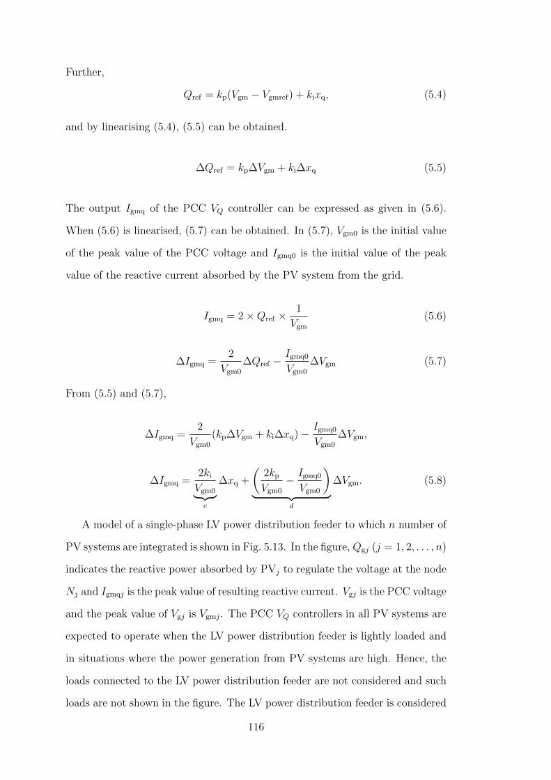
Further,
Qref = kp(Vgm − Vgmref) + kixq, (5.4)
and by linearising (5.4), (5.5) can be obtained.
∆Qref = kp∆Vgm + ki∆xq (5.5)
The output Igmq of the PCC VQ controller can be expressed as given in (5.6).
When (5.6) is linearised, (5.7) can be obtained. In (5.7), Vgm0 is the initial value
of the peak value of the PCC voltage and Igmq0 is the initial value of the peak
value of the reactive current absorbed by the PV system from the grid.
Igmq = 2×Qref ×1
Vgm
(5.6)
∆Igmq =2
Vgm0
∆Qref −Igmq0
Vgm0
∆Vgm (5.7)
From (5.5) and (5.7),
∆Igmq =2
Vgm0
(kp∆Vgm + ki∆xq)− Igmq0
Vgm0
∆Vgm,
∆Igmq =2ki
Vgm0︸ ︷︷ ︸c
∆xq +
(2kp
Vgm0
− Igmq0
Vgm0
)︸ ︷︷ ︸
d
∆Vgm. (5.8)
A model of a single-phase LV power distribution feeder to which n number of
PV systems are integrated is shown in Fig. 5.13. In the figure, Qgj (j = 1, 2, . . . , n)
indicates the reactive power absorbed by PVj to regulate the voltage at the node
Nj and Igmqj is the peak value of resulting reactive current. Vgj is the PCC voltage
and the peak value of Vgj is Vgmj. The PCC VQ controllers in all PV systems are
expected to operate when the LV power distribution feeder is lightly loaded and
in situations where the power generation from PV systems are high. Hence, the
loads connected to the LV power distribution feeder are not considered and such
loads are not shown in the figure. The LV power distribution feeder is considered
116
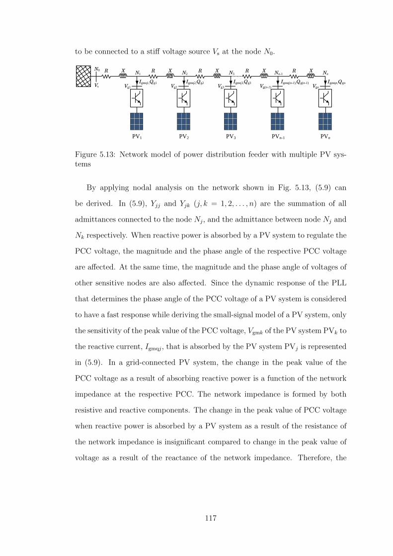
to be connected to a stiff voltage source Vs at the node N0.
XR
Vs
XR XR XR XR
PV1
N1 N2 N3 Nn-1 Nn
PV2 PV3 PVn-1 PVn
N0
Igmq1,Qg1Vg1 Vg2Igmq2,Qg2Vg3 Vg(n-1) VgnIgmq3,Qg3 Igmq(n-1),Qg(n-1) Igmqn,Qgn
Figure 5.13: Network model of power distribution feeder with multiple PV sys-tems
By applying nodal analysis on the network shown in Fig. 5.13, (5.9) can
be derived. In (5.9), Yjj and Yjk (j, k = 1, 2, . . . , n) are the summation of all
admittances connected to the node Nj, and the admittance between node Nj and
Nk respectively. When reactive power is absorbed by a PV system to regulate the
PCC voltage, the magnitude and the phase angle of the respective PCC voltage
are affected. At the same time, the magnitude and the phase angle of voltages of
other sensitive nodes are also affected. Since the dynamic response of the PLL
that determines the phase angle of the PCC voltage of a PV system is considered
to have a fast response while deriving the small-signal model of a PV system, only
the sensitivity of the peak value of the PCC voltage, Vgmk of the PV system PVk to
the reactive current, Igmqj, that is absorbed by the PV system PVj is represented
in (5.9). In a grid-connected PV system, the change in the peak value of the
PCC voltage as a result of absorbing reactive power is a function of the network
impedance at the respective PCC. The network impedance is formed by both
resistive and reactive components. The change in the peak value of PCC voltage
when reactive power is absorbed by a PV system as a result of the resistance of
the network impedance is insignificant compared to change in the peak value of
voltage as a result of the reactance of the network impedance. Therefore, the
117

admittance matrix [Y ] can be considered to be formed by the reactances only.
Igmq1
Igmq2
...
Igmqn
=
−Y11 Y12 . . . Y1n
Y21 −Y22 . . . Y2n
......
......
Yn1 Yn2 . . . −Ynn
︸ ︷︷ ︸
[Y ]
Vgm1
Vgm2
...
Vgmn
(5.9)
When (5.9) is linearised, (5.10) can be obtained.
∆Igmq1
∆Igmq2
...
∆Igmqn
=
−Y11 Y12 . . . Y1n
Y21 −Y22 . . . Y2n
......
......
Yn1 Yn2 . . . −Ynn
︸ ︷︷ ︸
[Y ]
∆Vgm1
∆Vgm2
...
∆Vgmn
(5.10)
The dynamic behaviour of the PCC VQ controller of the PV system PVj (j =
1, 2, . . . , n) can be represented by (5.8). The dynamic behaviour of PCC VQ con-
trollers in all of the PV systems shown in Fig. 5.13 can be represented in a matrix
form as given by (5.11).
∆Igmq1
∆Igmq2
...
∆Igmqn
︸ ︷︷ ︸
[∆IQ]
=
c1 0 . . . 0
0 c1 . . . 0
......
......
0 0 . . . cn
︸ ︷︷ ︸
[C]
∆xq1
∆xq2
...
∆xqn
︸ ︷︷ ︸
[∆XQ]
+
d1 0 . . . 0
0 d1 . . . 0
......
......
0 0 . . . dn
︸ ︷︷ ︸
[D]
∆Vgm1
∆Vgm2
...
∆Vgmn
︸ ︷︷ ︸
[∆VM]
(5.11)
By substituting (5.10) in (5.11), (5.12) can be obtained.
[∆VM] = [Y −D]−1[C][∆XQ] (5.12)
118
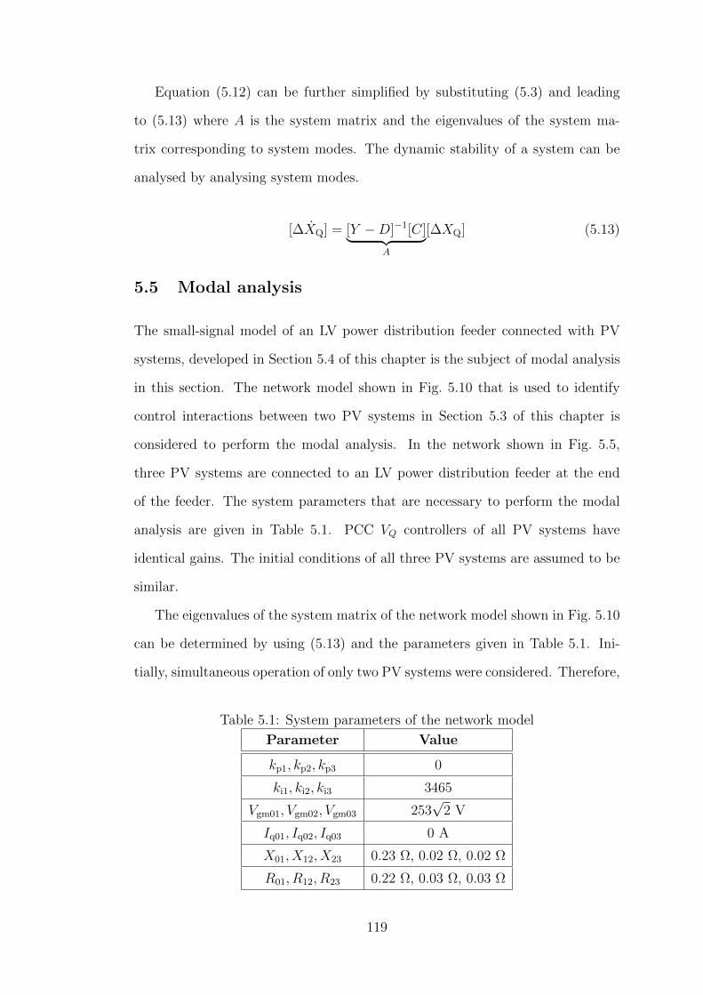
Equation (5.12) can be further simplified by substituting (5.3) and leading
to (5.13) where A is the system matrix and the eigenvalues of the system ma-
trix corresponding to system modes. The dynamic stability of a system can be
analysed by analysing system modes.
[∆XQ] = [Y −D]−1[C]︸ ︷︷ ︸A
[∆XQ] (5.13)
5.5 Modal analysis
The small-signal model of an LV power distribution feeder connected with PV
systems, developed in Section 5.4 of this chapter is the subject of modal analysis
in this section. The network model shown in Fig. 5.10 that is used to identify
control interactions between two PV systems in Section 5.3 of this chapter is
considered to perform the modal analysis. In the network shown in Fig. 5.5,
three PV systems are connected to an LV power distribution feeder at the end
of the feeder. The system parameters that are necessary to perform the modal
analysis are given in Table 5.1. PCC VQ controllers of all PV systems have
identical gains. The initial conditions of all three PV systems are assumed to be
similar.
The eigenvalues of the system matrix of the network model shown in Fig. 5.10
can be determined by using (5.13) and the parameters given in Table 5.1. Ini-
tially, simultaneous operation of only two PV systems were considered. Therefore,
Table 5.1: System parameters of the network model
Parameter Value
kp1, kp2, kp3 0
ki1, ki2, ki3 3465
Vgm01, Vgm02, Vgm03 253√
2 V
Iq01, Iq02, Iq03 0 A
X01, X12, X23 0.23 Ω, 0.02 Ω, 0.02 Ω
R01, R12, R23 0.22 Ω, 0.03 Ω, 0.03 Ω
119

modal analysis was performed considering that PV1 of Fig. 5.10 was disconnected
from the network. The corresponding eigenvalues obtained are given in (5.14).
According to the eigenvalues obtained, there are no oscillatory modes in the sys-
tem since all modes are critically damped. The critical mode is λ22 as that is
closer to the origin in the complex plane than λ12.
λ12
λ22
=
−8.96
−0.24
(5.14)
The time-domain response of the critical mode of (5.14) is shown in Fig. 5.14
for a step change in the system. The dynamic characteristics of the critical mode
shown in Fig. 5.14 is similar to the slow dynamic variation that can be seen in
Fig. 5.6(b). Hence, the presence of control interactions between PV systems that
is identified in Section 5.3 is mathematically verified by the modal analysis.
The eigenvalues obtained considering all three PV systems were connected to
the grid are given in (5.15). According to the results, the critical mode, that is
λ33, results PV systems to reach steady-state after about 60 s. However, such
fact is not verifiable by results shown in Fig. 5.11(b) since the PCC VQ controller
of a PV system had been saturated at zero.
0 5 10 15 20 25 300
0.2
0.4
0.6
0.8
1
Time (sec)
Am
plitu
de
Figure 5.14: Time-domain response of the critical mode
120
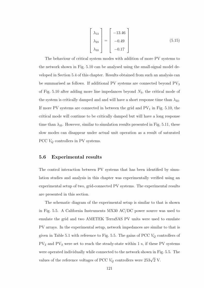
λ13
λ23
λ33
=
−13.46
−0.49
−0.17
(5.15)
The behaviour of critical system modes with addition of more PV systems to
the network shown in Fig. 5.10 can be analysed using the small-signal model de-
veloped in Section 5.4 of this chapter. Results obtained from such an analysis can
be summarised as follows. If additional PV systems are connected beyond PV3
of Fig. 5.10 after adding more line impedances beyond N3, the critical mode of
the system is critically damped and and will have a short response time than λ33.
If more PV systems are connected in between the grid and PV1 in Fig. 5.10, the
critical mode will continue to be critically damped but will have a long response
time than λ33. However, similar to simulation results presented in Fig. 5.11, these
slow modes can disappear under actual unit operation as a result of saturated
PCC VQ controllers in PV systems.
5.6 Experimental results
The control interaction between PV systems that has been identified by simu-
lation studies and analysis in this chapter was experimentally verified using an
experimental setup of two, grid-connected PV systems. The experimental results
are presented in this section.
The schematic diagram of the experimental setup is similar to that is shown
in Fig. 5.5. A California Instruments MX30 AC/DC power source was used to
emulate the grid and two AMETEK TerraSAS PV units were used to emulate
PV arrays. In the experimental setup, network impedances are similar to that is
given in Table 5.1 with reference to Fig. 5.5. The gains of PCC VQ controllers of
PV2 and PV3 were set to reach the steady-state within 1 s, if these PV systems
were operated individually while connected to the network shown in Fig. 5.5. The
values of the reference voltages of PCC VQ controllers were 253√
2 V.
121
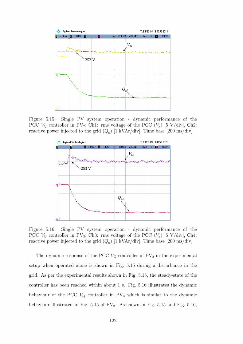
Vg2
253 V
Qg2
Figure 5.15: Single PV system operation - dynamic performance of thePCC VQ controller in PV2: Ch1: rms voltage of the PCC (Vg) [5 V/div], Ch2:reactive power injected to the grid (Qg) [1 kVAr/div], Time base [200 ms/div]
PCC
Two-stage converter
LCL filter DS1104 controller
Feedback signals
Switching signals
Vg3
253 V
Qg3
Figure 5.16: Single PV system operation - dynamic performance of thePCC VQ controller in PV3: Ch3: rms voltage of the PCC (Vg) [5 V/div], Ch4:reactive power injected to the grid (Qg) [1 kVAr/div], Time base [200 ms/div]
The dynamic response of the PCC VQ controller in PV2 in the experimental
setup when operated alone is shown in Fig. 5.15 during a disturbance in the
grid. As per the experimental results shown in Fig. 5.15, the steady-state of the
controller has been reached within about 1 s. Fig. 5.16 illustrates the dynamic
behaviour of the PCC VQ controller in PV3 which is similar to the dynamic
behaviour illustrated in Fig. 5.15 of PV2. As shown in Fig. 5.15 and Fig. 5.16,
122
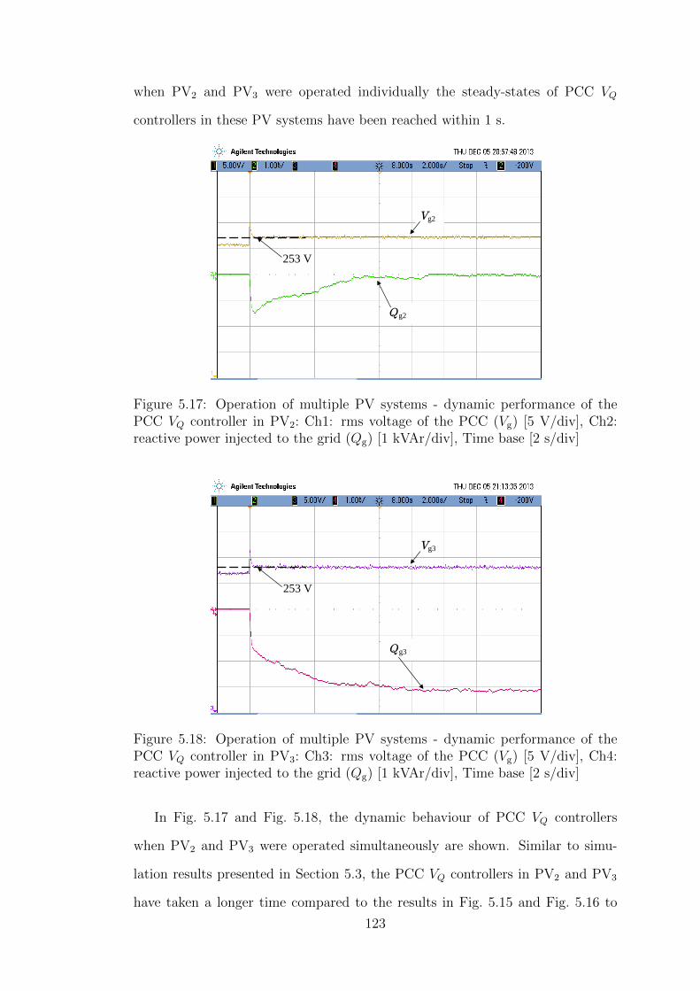
when PV2 and PV3 were operated individually the steady-states of PCC VQ
controllers in these PV systems have been reached within 1 s.
Vg2
253 V
Qg2
Figure 5.17: Operation of multiple PV systems - dynamic performance of thePCC VQ controller in PV2: Ch1: rms voltage of the PCC (Vg) [5 V/div], Ch2:reactive power injected to the grid (Qg) [1 kVAr/div], Time base [2 s/div]
Vg3
253 V
Qg3
Figure 5.18: Operation of multiple PV systems - dynamic performance of thePCC VQ controller in PV3: Ch3: rms voltage of the PCC (Vg) [5 V/div], Ch4:reactive power injected to the grid (Qg) [1 kVAr/div], Time base [2 s/div]
In Fig. 5.17 and Fig. 5.18, the dynamic behaviour of PCC VQ controllers
when PV2 and PV3 were operated simultaneously are shown. Similar to simu-
lation results presented in Section 5.3, the PCC VQ controllers in PV2 and PV3
have taken a longer time compared to the results in Fig. 5.15 and Fig. 5.16 to
123
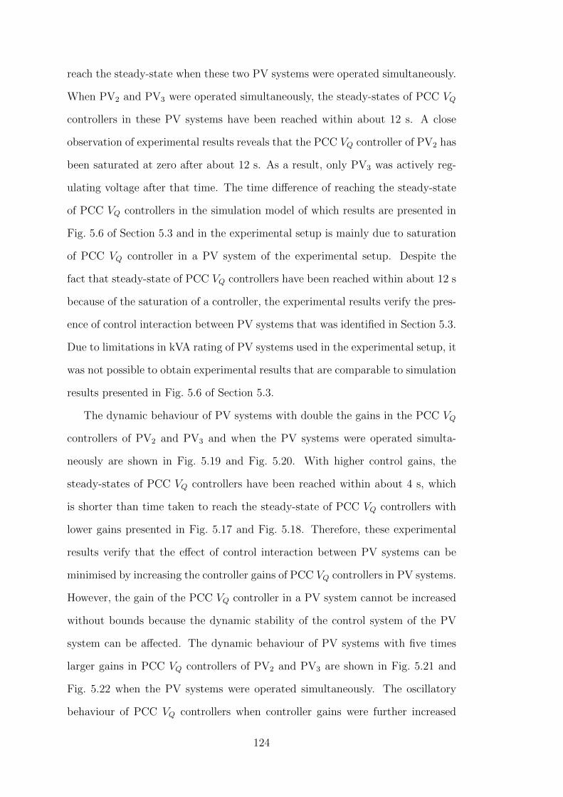
reach the steady-state when these two PV systems were operated simultaneously.
When PV2 and PV3 were operated simultaneously, the steady-states of PCC VQ
controllers in these PV systems have been reached within about 12 s. A close
observation of experimental results reveals that the PCC VQ controller of PV2 has
been saturated at zero after about 12 s. As a result, only PV3 was actively reg-
ulating voltage after that time. The time difference of reaching the steady-state
of PCC VQ controllers in the simulation model of which results are presented in
Fig. 5.6 of Section 5.3 and in the experimental setup is mainly due to saturation
of PCC VQ controller in a PV system of the experimental setup. Despite the
fact that steady-state of PCC VQ controllers have been reached within about 12 s
because of the saturation of a controller, the experimental results verify the pres-
ence of control interaction between PV systems that was identified in Section 5.3.
Due to limitations in kVA rating of PV systems used in the experimental setup, it
was not possible to obtain experimental results that are comparable to simulation
results presented in Fig. 5.6 of Section 5.3.
The dynamic behaviour of PV systems with double the gains in the PCC VQ
controllers of PV2 and PV3 and when the PV systems were operated simulta-
neously are shown in Fig. 5.19 and Fig. 5.20. With higher control gains, the
steady-states of PCC VQ controllers have been reached within about 4 s, which
is shorter than time taken to reach the steady-state of PCC VQ controllers with
lower gains presented in Fig. 5.17 and Fig. 5.18. Therefore, these experimental
results verify that the effect of control interaction between PV systems can be
minimised by increasing the controller gains of PCC VQ controllers in PV systems.
However, the gain of the PCC VQ controller in a PV system cannot be increased
without bounds because the dynamic stability of the control system of the PV
system can be affected. The dynamic behaviour of PV systems with five times
larger gains in PCC VQ controllers of PV2 and PV3 are shown in Fig. 5.21 and
Fig. 5.22 when the PV systems were operated simultaneously. The oscillatory
behaviour of PCC VQ controllers when controller gains were further increased
124
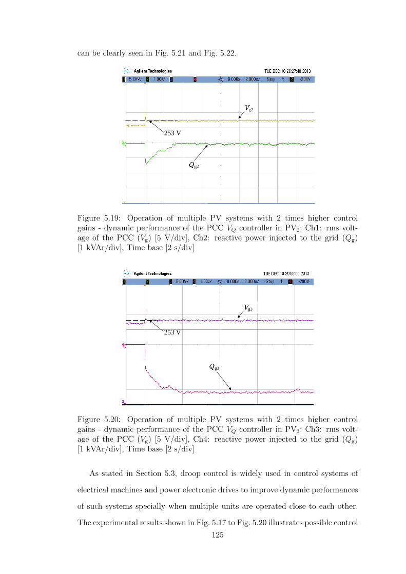
can be clearly seen in Fig. 5.21 and Fig. 5.22.
Vg2
253 V
Qg2
Figure 5.19: Operation of multiple PV systems with 2 times higher controlgains - dynamic performance of the PCC VQ controller in PV2: Ch1: rms volt-age of the PCC (Vg) [5 V/div], Ch2: reactive power injected to the grid (Qg)[1 kVAr/div], Time base [2 s/div]
Vg3
253 V
Qg3
Figure 5.20: Operation of multiple PV systems with 2 times higher controlgains - dynamic performance of the PCC VQ controller in PV3: Ch3: rms volt-age of the PCC (Vg) [5 V/div], Ch4: reactive power injected to the grid (Qg)[1 kVAr/div], Time base [2 s/div]
As stated in Section 5.3, droop control is widely used in control systems of
electrical machines and power electronic drives to improve dynamic performances
of such systems specially when multiple units are operated close to each other.
The experimental results shown in Fig. 5.17 to Fig. 5.20 illustrates possible control
125
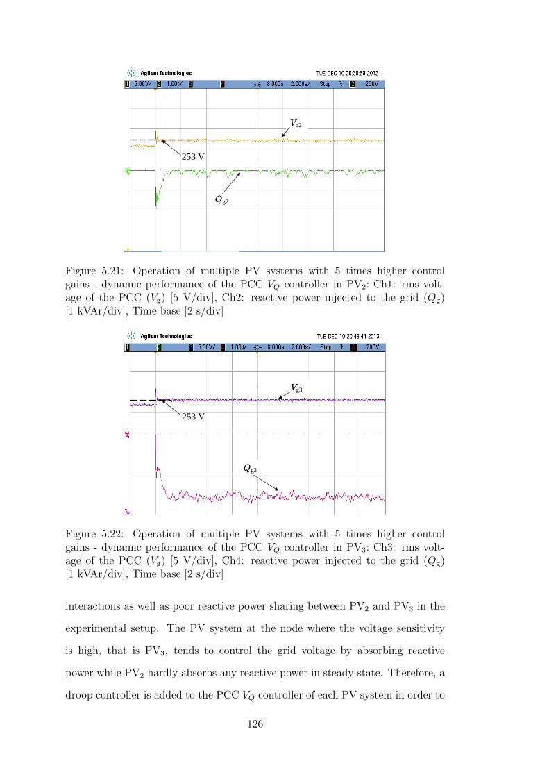
Vg2
253 V
Qg2
Figure 5.21: Operation of multiple PV systems with 5 times higher controlgains - dynamic performance of the PCC VQ controller in PV2: Ch1: rms volt-age of the PCC (Vg) [5 V/div], Ch2: reactive power injected to the grid (Qg)[1 kVAr/div], Time base [2 s/div]
PV simulator
PV1 PV2
Vg3
253 V
Qg3
Figure 5.22: Operation of multiple PV systems with 5 times higher controlgains - dynamic performance of the PCC VQ controller in PV3: Ch3: rms volt-age of the PCC (Vg) [5 V/div], Ch4: reactive power injected to the grid (Qg)[1 kVAr/div], Time base [2 s/div]
interactions as well as poor reactive power sharing between PV2 and PV3 in the
experimental setup. The PV system at the node where the voltage sensitivity
is high, that is PV3, tends to control the grid voltage by absorbing reactive
power while PV2 hardly absorbs any reactive power in steady-state. Therefore, a
droop controller is added to the PCC VQ controller of each PV system in order to
126
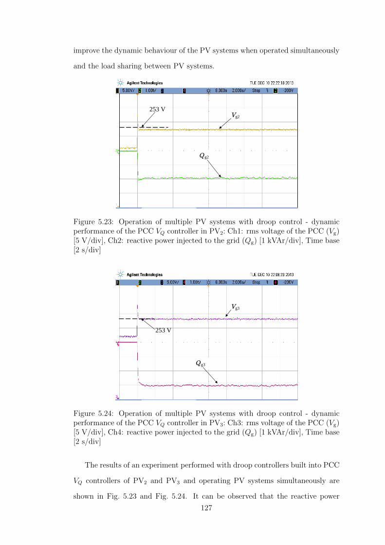
improve the dynamic behaviour of the PV systems when operated simultaneously
and the load sharing between PV systems.
Vg2 253 V
Qg2
PV simulator
PV1 PV2
Figure 5.23: Operation of multiple PV systems with droop control - dynamicperformance of the PCC VQ controller in PV2: Ch1: rms voltage of the PCC (Vg)[5 V/div], Ch2: reactive power injected to the grid (Qg) [1 kVAr/div], Time base[2 s/div]
Vg3
253 V
Qg3
Figure 5.24: Operation of multiple PV systems with droop control - dynamicperformance of the PCC VQ controller in PV3: Ch3: rms voltage of the PCC (Vg)[5 V/div], Ch4: reactive power injected to the grid (Qg) [1 kVAr/div], Time base[2 s/div]
The results of an experiment performed with droop controllers built into PCC
VQ controllers of PV2 and PV3 and operating PV systems simultaneously are
shown in Fig. 5.23 and Fig. 5.24. It can be observed that the reactive power
127

sharing between PV systems has been improved. Further, the steady-states of
the PCC VQ controllers have been reached within about 2 s. The experimental
results confirm that a droop controller built into the PCC VQ controller of a PV
system is able to improve reactive power sharing between multiple PV systems
and minimise the effect of control interactions.
Further experimental studies were carried out by considering different oper-
ating conditions of PV systems and also by integrating commercially available
small-scale DSTATCOMs to the experimental setup. The results of such exper-
imental studies are discussed in Appendix E of this Thesis. These experimental
results do not indicate any dynamic interaction between converter systems that
may impact the stable operation.
5.7 Chapter summary
In this chapter, the control interactions between multiple PV systems were iden-
tified by simulation studies performed. The PV systems considered in this re-
search are interfaced to the grid via current-controlled voltage source converters.
A small-signal model of a power distribution feeder to which multiple PV systems
are integrated was developed while considering practical techniques used to es-
tablish the control system of a grid-connected PV system described in Chapter 3
and Chapter 4. Modal analysis was performed by using the developed small-
signal model to verify the simulation results. The small-signal model developed
in the current research was used to analyse the dynamic stability and system level
behaviour of multiple PV systems that control the grid voltage dynamically. The
accuracy of the small-signal model developed and simulation results presented in
this chapter was verified using experimental results. Based on the simulation and
experimental results presented and mathematical derivations in this chapter, the
following conclusions can be drawn.
• The results of time-domain simulation studies of an LV power grid to which
128

multiple solar PV systems are integrated presented in this chapter, confirm
that control interaction between multiple PV systems can exist when those
systems regulate the respective PCC voltage dynamically by absorbing re-
active power from the grid.
• The small-signal model of a multiple PV installation developed in this chap-
ter is accurate and can be used to analyse the control interaction between
multiple PV systems and to investigate the level of sensitivity of different
parameters.
• The control interactions between multiple PV systems that is identified
in this research does not cause any dynamic instability in the grid since
all modes are critically damped, as demonstrated by the modal analysis
performed.
• The effects of control interaction identified in the current research can be
minimised by adding a droop controller to the dynamic PCC voltage con-
troller of a PV system. Further, such a droop controller improves reactive
power sharing between multiple PV systems.
The research outcomes presented in this chapter confirm that dynamic insta-
bility of the grid as result of control interaction between grid-connected multiple
PV systems that control the PCC voltage with dynamic reactive power controllers
is unlikely to occur. Therefore, multiple PV systems that dynamically control the
PCC voltage can be deployed to control the voltage of a power distribution feeder
without concerns.
129

130
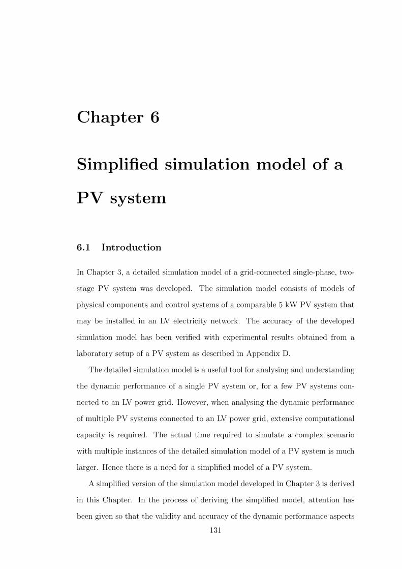
Chapter 6
Simplified simulation model of a
PV system
6.1 Introduction
In Chapter 3, a detailed simulation model of a grid-connected single-phase, two-
stage PV system was developed. The simulation model consists of models of
physical components and control systems of a comparable 5 kW PV system that
may be installed in an LV electricity network. The accuracy of the developed
simulation model has been verified with experimental results obtained from a
laboratory setup of a PV system as described in Appendix D.
The detailed simulation model is a useful tool for analysing and understanding
the dynamic performance of a single PV system or, for a few PV systems con-
nected to an LV power grid. However, when analysing the dynamic performance
of multiple PV systems connected to an LV power grid, extensive computational
capacity is required. The actual time required to simulate a complex scenario
with multiple instances of the detailed simulation model of a PV system is much
larger. Hence there is a need for a simplified model of a PV system.
A simplified version of the simulation model developed in Chapter 3 is derived
in this Chapter. In the process of deriving the simplified model, attention has
been given so that the validity and accuracy of the dynamic performance aspects
131
are not compromised. The strategy that was adopted to simplify the detailed
simulation model of the PV system is described and the dynamic performance of
the detailed and simplified simulation models are compared.
6.2 Simplified model of a PV system
The PV system in the detailed simulation model developed in Chapter 3 was
interfaced to the grid via a current-controlled VSC. Such a converter system can
be modelled using a controlled current source. Therefore, in the simplified model,
the PV system can be represented by a controlled current source.
There are several layers of control in a grid-connected PV system as described
in Chapters 3 and 4. The control systems of the inner layers respond faster
than the control systems of the outer layers to ensure the dynamic stability of
the total control system and the overall dynamic performance of a PV system
is determined by the dynamic performance of the outer control loops. Hence, if
the characteristics of control systems in the outer layers are of primary interest
with regard to the overall dynamic behaviour of the PV system, the inner control
systems can be disregarded in the simplified model.
A simplified model of a PV system as suitable for analysing the dynamic per-
formance of multiple PV systems connected to an LV power grid is developed. The
intended use of this model is to identify possible dynamic interactions between
multiple PV systems when each PV system is dynamically regulating its PCC
voltage with the PCC voltage controllers developed in Chapter 4. As described
in Chapter 4, the dynamic PCC voltage controllers, i.e. the PCC VQ controller
and PCC VP controller, are at the most outer layers of the control for a PV sys-
tem and determine the overall dynamic performance of the PV system. Hence,
in the simplified model of a PV system, the dynamic behaviour of PCC voltage
controllers are accurately presented while disregarding the dynamic behaviour of
control systems in the inner layers such as the current controller, the DC-link
voltage controller and the controller of the DC-DC boost converter.
132
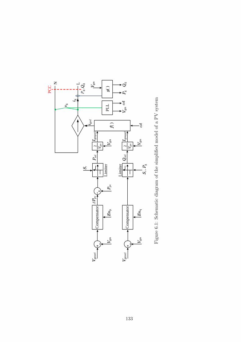
Vgm2
Vgm2Q
ref
Pre
f
Lim
iter
Lim
iter
Vgm
Vgm
refI g
mpr
efC
ompe
nsat
or
Vgm
Vgm
ref
Com
pens
ator
Ppv
Δ Ppv
Vgm
Vgm
LN
Sr
Sr , P
g
En
p
En
q
f ( )
v g
PLL
Vgmω t
ω t
i g
g( )V
gm
PgQ
g
i gre
f
PCC
P g ,Q
g
I gm
qref
Fig
ure
6.1:
Sch
emat
icdia
gram
ofth
esi
mplified
model
ofa
PV
syst
em
133

An illustration of the simplified model of a PV system is shown in Fig. 6.1.
The PLL structure used in the simplified model of the PV system is similar to
that of the detailed model of a PV system developed in Chapter 3. The measured
PCC voltage, vg, is an input to the PLL. The peak value of vg, Vgm, and the phase
angle of vg, ωt, are the outputs of the PLL. The rms value of vg is Vg.
In order to calculate the active and reactive power injected to the grid, Pg
and Qg respectively, the current injected to the grid by the PV system, ig, is
measured. The signal processing block denoted by g( ) in Fig. 6.1 represents
the mathematical calculations performed to determine Pg and Qg. In the signal
processing block g( ), the measured current ig is passed through a band-pass
filter, a scaled integrator and a Park transformation (αβ to dq transformation)
block similar to that which is done to the measured voltage at the PCC, vg, in
the PLL. The output of the Park transformation block in g( ) is the peak value
of the active current component of ig, Igmp, and the peak value of the reactive
current component of ig, Igmq. In g( ), Pg and Qg are determined by using Vgm,
Igmp and Igmq as given in (6.1) and (6.2) respectively.
Pg =1
2VgmIgmp (6.1)
Qg = −1
2VgmIgmq (6.2)
In the simplified model of a PV system, other than the PLL, only dynamic
PCC voltage controllers, i.e. the PCC VQ controller and PCC VP controller
developed in Chapter 4, are implemented. In the PCC VQ controller in Fig. 6.1,
Vgmref is the reference voltage. The controller enable signal, Enq, represents
conditions under which the dynamic voltage regulation is enabled, for an example,
a defined PCC voltage above which the controller is responsive. The limiter is
used to limit the reactive power injection to the available capacity of the VSC that
interfaces the PV system to the grid or to limit the allowed maximum reactive
power injection to the grid at a given time. Sr is the apparent power capacity of
134
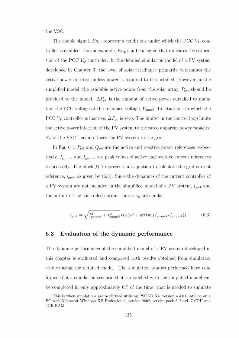
the VSC.
The enable signal, Enp, represents conditions under which the PCC VP con-
troller is enabled. For an example, Enp can be a signal that indicates the satura-
tion of the PCC VQ controller. In the detailed simulation model of a PV system
developed in Chapter 3, the level of solar irradiance primarily determines the
active power injection unless power is required to be curtailed. However, in the
simplified model, the available active power from the solar array, Ppv, should be
provided to the model. ∆Ppv is the amount of active power curtailed to main-
tain the PCC voltage at the reference voltage, Vgmref . In situations in which the
PCC VP controller is inactive, ∆Ppv is zero. The limiter in the control loop limits
the active power injection of the PV system to the rated apparent power capacity,
Sr, of the VSC that interfaces the PV system to the grid.
In Fig. 6.1, Pref and Qref are the active and reactive power references respec-
tively. Igmpref and Igmqref are peak values of active and reactive current references
respectively. The block f( ) represents an equation to calculate the grid current
reference, igref , as given by (6.3). Since the dynamics of the current controller of
a PV system are not included in the simplified model of a PV system, igref and
the output of the controlled current source, ig are similar.
igref =√I2
gmpref + I2gmqref cos(ωt+ arctan(Igmqref/Igmpref)) (6.3)
6.3 Evaluation of the dynamic performance
The dynamic performance of the simplified model of a PV system developed in
this chapter is evaluated and compared with results obtained from simulation
studies using the detailed model. The simulation studies performed have con-
firmed that a simulation scenario that is modelled with the simplified model can
be completed in only approximately 6% of the time1 that is needed to simulate
1This is when simulations are performed utilising PSCAD X4, version 4.4.0.0 intalled on aPC with Microsoft Windows XP Professional, version 2002, service pack 3, Intel i7 CPU and4GB RAM.
135

a comparable simulation scenario utlising the detailed model of a PV system.
In this section, the dynamic performance of the detailed model of a PV system
integrated with dynamic PCC voltage controllers developed in Chapter 4 and the
dynamic performance of the simplified model of a PV system developed in this
chapter are compared. In most of the graphs presented in this section, there are
three traces: a variation of a measured parameter in the detailed model of a PV
system during a simulation case, the variation of the same parameter in the sim-
plified model of a PV system during a similar simulation case and the difference
between the two variations.
0.8 0.9 1 1.1 1.2 1.3−30−18−66
1830
i g(A
)
0.8 0.9 1 1.1 1.2 1.3−10−6−22610
i gERROR
(A)
(a)
0.8 0.9 1 1.1 1.2 1.3230234238242246250
Vg(V
)
0.8 0.9 1 1.1 1.2 1.3−10−6−22610
VgERROR
(V)
(b)
0.8 0.9 1 1.1 1.2 1.3−2
−1
0
1
Qg(kVAr)
0.8 0.9 1 1.1 1.2 1.3−0.6
−0.2
0.2
0.6
QgERROR
(kVAr)
(d)Time (s)
Detailed model Simplified model Error
0.8 0.9 1 1.1 1.2 1.3−6−5−4−3−2−10
Pg(kW
)
0.8 0.9 1 1.1 1.2 1.3−1.2−0.8−0.400.40.81.2
PgERROR
(kW
)
(c)
Figure 6.2: Dynamic response of the detailed and simplified model of a PV systemduring step changes in active power reference and reactive power reference
The dynamic behaviour of the detailed model of a PV system and the sim-
plified model of a PV system during step changes of active and reactive power
136
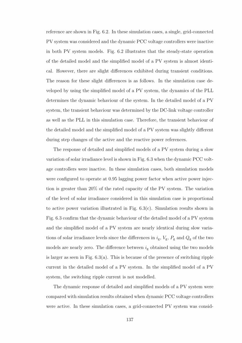
reference are shown in Fig. 6.2. In these simulation cases, a single, grid-connected
PV system was considered and the dynamic PCC voltage controllers were inactive
in both PV system models. Fig. 6.2 illustrates that the steady-state operation
of the detailed model and the simplified model of a PV system is almost identi-
cal. However, there are slight differences exhibited during transient conditions.
The reason for these slight differences is as follows. In the simulation case de-
veloped by using the simplified model of a PV system, the dynamics of the PLL
determines the dynamic behaviour of the system. In the detailed model of a PV
system, the transient behaviour was determined by the DC-link voltage controller
as well as the PLL in this simulation case. Therefore, the transient behaviour of
the detailed model and the simplified model of a PV system was slightly different
during step changes of the active and the reactive power references.
The response of detailed and simplified models of a PV system during a slow
variation of solar irradiance level is shown in Fig. 6.3 when the dynamic PCC volt-
age controllers were inactive. In these simulation cases, both simulation models
were configured to operate at 0.95 lagging power factor when active power injec-
tion is greater than 20% of the rated capacity of the PV system. The variation
of the level of solar irradiance considered in this simulation case is proportional
to active power variation illustrated in Fig. 6.3(c). Simulation results shown in
Fig. 6.3 confirm that the dynamic behaviour of the detailed model of a PV system
and the simplified model of a PV system are nearly identical during slow varia-
tions of solar irradiance levels since the differences in ig, Vg, Pg and Qg of the two
models are nearly zero. The difference between ig obtained using the two models
is larger as seen in Fig. 6.3(a). This is because of the presence of switching ripple
current in the detailed model of a PV system. In the simplified model of a PV
system, the switching ripple current is not modelled.
The dynamic response of detailed and simplified models of a PV system were
compared with simulation results obtained when dynamic PCC voltage controllers
were active. In these simulation cases, a grid-connected PV system was consid-
137
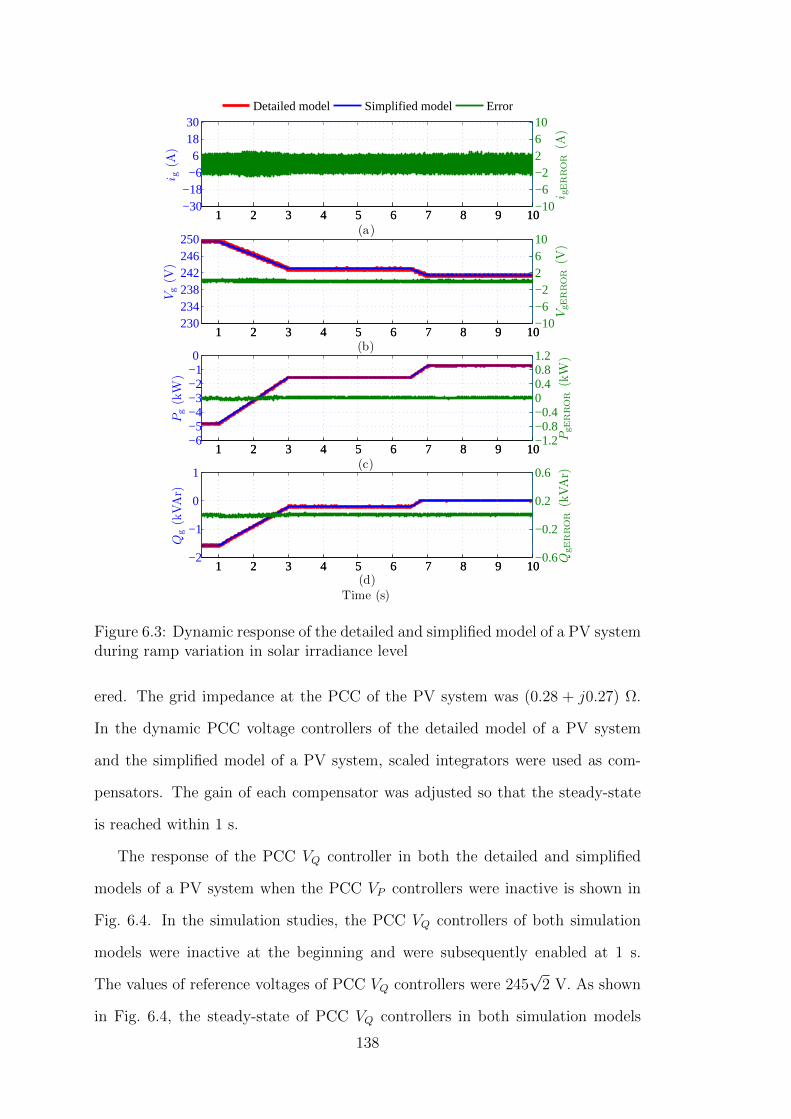
1 2 3 4 5 6 7 8 9 10−30−18−66
1830
i g(A
)
1 2 3 4 5 6 7 8 9 10−10−6−22610
i gERROR
(A)
(a)
1 2 3 4 5 6 7 8 9 10230234238242246250
Vg(V
)
1 2 3 4 5 6 7 8 9 10−10−6−22610
VgERROR
(V)
(b)
1 2 3 4 5 6 7 8 9 10−2
−1
0
1
Qg(kVAr)
1 2 3 4 5 6 7 8 9 10−0.6
−0.2
0.2
0.6
QgERROR
(kVAr)
(d)Time (s)
Detailed model Simplified model Error
1 2 3 4 5 6 7 8 9 10−6−5−4−3−2−10
Pg(kW
)
1 2 3 4 5 6 7 8 9 10−1.2−0.8−0.400.40.81.2
PgERROR
(kW
)
(c)
Figure 6.3: Dynamic response of the detailed and simplified model of a PV systemduring ramp variation in solar irradiance level
ered. The grid impedance at the PCC of the PV system was (0.28 + j0.27) Ω.
In the dynamic PCC voltage controllers of the detailed model of a PV system
and the simplified model of a PV system, scaled integrators were used as com-
pensators. The gain of each compensator was adjusted so that the steady-state
is reached within 1 s.
The response of the PCC VQ controller in both the detailed and simplified
models of a PV system when the PCC VP controllers were inactive is shown in
Fig. 6.4. In the simulation studies, the PCC VQ controllers of both simulation
models were inactive at the beginning and were subsequently enabled at 1 s.
The values of reference voltages of PCC VQ controllers were 245√
2 V. As shown
in Fig. 6.4, the steady-state of PCC VQ controllers in both simulation models
138

0.5 1 1.5 2 2.5 3−30−18−66
1830
i g(A
)0.5 1 1.5 2 2.5 3
−10−6−22610
i gERROR
(A)
(a)
0.5 1 1.5 2 2.5 3230234238242246250
Vg(V
)
0.5 1 1.5 2 2.5 3−10−6−22610
VgERROR
(V)
(b)
0.5 1 1.5 2 2.5 3−3
−2
−1
0
1
Qg(kVAr)
0.5 1 1.5 2 2.5 3−0.6
−0.3
0
0.3
0.6
QgERROR
(kVAr)
(d)Time (s)
Detailed model Simplified model Error
0.5 1 1.5 2 2.5 3−6−5−4−3−2−10
Pg(kW
)
0.5 1 1.5 2 2.5 3−1.2−0.8−0.400.40.81.2
PgERROR
(kW
)
(c)
Figure 6.4: Dynamic performance of the PCC VQ controller in the simplifiedmodel of a PV system and the detailed model of a PV system
has been reached within 1 s. Further, simulation results shown in Fig. 6.4 con-
firms that PCC VQ controllers in both simulation models have similar dynamic
behaviours.
The response of PCC VP controllers of both the detailed and simplified models
of a PV system when PCC VQ controllers were inactive is shown in Fig. 6.5.
Though the steady-state of PCC VP controllers has been reached within 1 s, the
transient behaviour of PCC VP controllers in both models are slightly different
as can be observed in Fig. 6.5.
The difference in the transient behaviour of PCC VP controllers in detailed
and simplified models of a PV system shown in Fig. 6.5 can be explained as
follows. In the detailed model of a PV system, when active power is curtailed
139
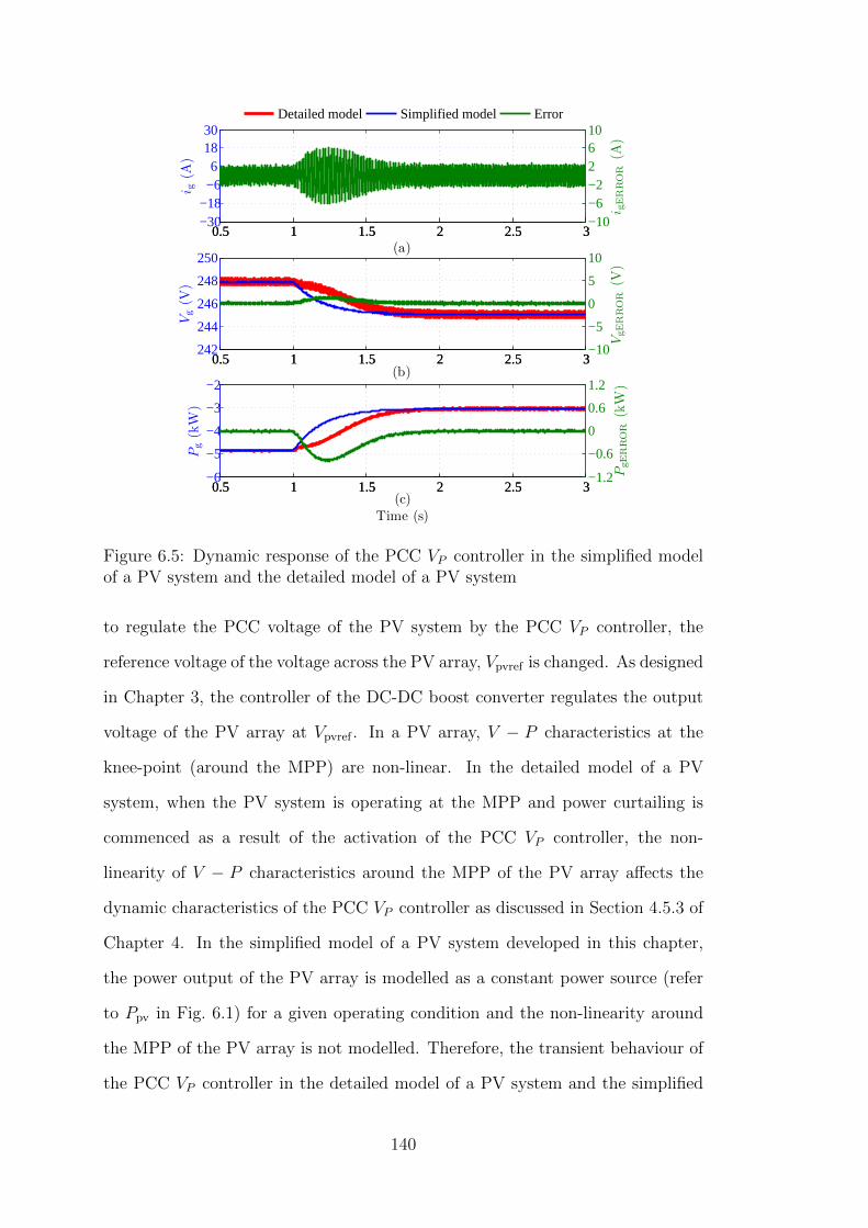
0.5 1 1.5 2 2.5 3−30−18−66
1830
i g(A
)
0.5 1 1.5 2 2.5 3−10−6−22610
i gERROR
(A)
(a)
0.5 1 1.5 2 2.5 3242
244
246
248
250
Vg(V
)
0.5 1 1.5 2 2.5 3−10
−5
0
5
10
VgERROR
(V)
(b)
Detailed model Simplified model Error
0.5 1 1.5 2 2.5 3−6
−5
−4
−3
−2
Pg(kW
)
0.5 1 1.5 2 2.5 3−1.2
−0.6
0
0.6
1.2
PgERROR
(kW
)
(c)Time (s)
Figure 6.5: Dynamic response of the PCC VP controller in the simplified modelof a PV system and the detailed model of a PV system
to regulate the PCC voltage of the PV system by the PCC VP controller, the
reference voltage of the voltage across the PV array, Vpvref is changed. As designed
in Chapter 3, the controller of the DC-DC boost converter regulates the output
voltage of the PV array at Vpvref . In a PV array, V − P characteristics at the
knee-point (around the MPP) are non-linear. In the detailed model of a PV
system, when the PV system is operating at the MPP and power curtailing is
commenced as a result of the activation of the PCC VP controller, the non-
linearity of V − P characteristics around the MPP of the PV array affects the
dynamic characteristics of the PCC VP controller as discussed in Section 4.5.3 of
Chapter 4. In the simplified model of a PV system developed in this chapter,
the power output of the PV array is modelled as a constant power source (refer
to Ppv in Fig. 6.1) for a given operating condition and the non-linearity around
the MPP of the PV array is not modelled. Therefore, the transient behaviour of
the PCC VP controller in the detailed model of a PV system and the simplified
140

model of a PV system is marginally different.
VsInfinite grid
XgRg XRN1 N2
PV1 PV2
N0
Figure 6.6: Two PV systems connected to an LV power grid
Simulation studies were performed using detailed and simplified models of a
PV system to determine the suitability of using the simplified model of a PV
system developed in this chapter to model an LV power grid integrated with mul-
tiple PV systems and for identifying dynamic interactions between PV systems.
In these simulation studies, the network model shown in Fig. 6.6 was consid-
ered. In the network model shown in Fig. 6.6, (Rg + jXg) is (0.25 + j0.25) Ω
and (R + jX) is (0.03 + j0.02) Ω. The PCC VQ controllers of two PV systems
shown in Fig. 6.6 were active and PCC VP controllers were inactive. The gains
of PCC VQ controllers of two PV systems were identical.
Results obtained from two simulation cases by modelling the network shown
in Fig. 6.6 by using detailed and simplified models of a PV system are shown in
Fig. 6.7 and Fig. 6.8. The PCC VQ controllers of PV1 and PV2 were configured to
reach the steady-state within 1 s if those PV systems were operated individually
and when those were connected to the grid as shown in Fig. 6.6. As per the sim-
ulation results presented in Fig. 6.7 and Fig. 6.8, the dynamic behaviours of both
detailed and simplified models of a PV system are identical in these simulation
cases. The simulation results shown in Fig. 6.7 and Fig. 6.8 are of initial 10 s
of the simulation study. At that time PCC VQ controllers had not reached the
steady-state. The steady-state of PCC VQ controllers of PV1 and PV2 reached
within about 30 s. The time taken to reach the steady-state of PCC VQ controllers
when these PV systems were operated simultaneously is longer than the time to
141
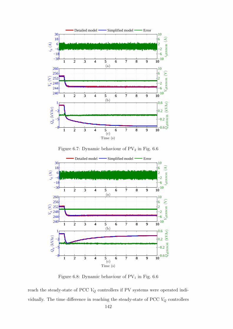
1 2 3 4 5 6 7 8 9 10−30−18−66
1830
i g(A
)
1 2 3 4 5 6 7 8 9 10−10−6−22610
i gERROR
(A)
(a)
1 2 3 4 5 6 7 8 9 10240244248252256260
Vg(V
)
1 2 3 4 5 6 7 8 9 10−10−6−22610
VgERROR
(V)
(b)
1 2 3 4 5 6 7 8 9 10−8
−5
−2
1
Qg(kVAr)
1 2 3 4 5 6 7 8 9 10−0.6
−0.2
0.2
0.6
QgERROR
(kVAr)
(c)Time (s)
Detailed model Simplified model Error
Figure 6.7: Dynamic behaviour of PV2 in Fig. 6.6
1 2 3 4 5 6 7 8 9 10−30−18−66
1830
i g(A
)
1 2 3 4 5 6 7 8 9 10−10−6−22610
i gERROR
(A)
(a)
1 2 3 4 5 6 7 8 9 10240244248252256260
Vg(V
)
1 2 3 4 5 6 7 8 9 10−10−6−22610
VgERROR
(V)
(b)
1 2 3 4 5 6 7 8 9 10−8
−5
−2
1
Qg(kVAr)
1 2 3 4 5 6 7 8 9 10−0.6
−0.2
0.2
0.6
QgERROR
(kVAr)
(c)Time (s)
Detailed model Simplified model Error
Figure 6.8: Dynamic behaviour of PV1 in Fig. 6.6
reach the steady-state of PCC VQ controllers if PV systems were operated indi-
vidually. The time difference in reaching the steady-state of PCC VQ controllers
142
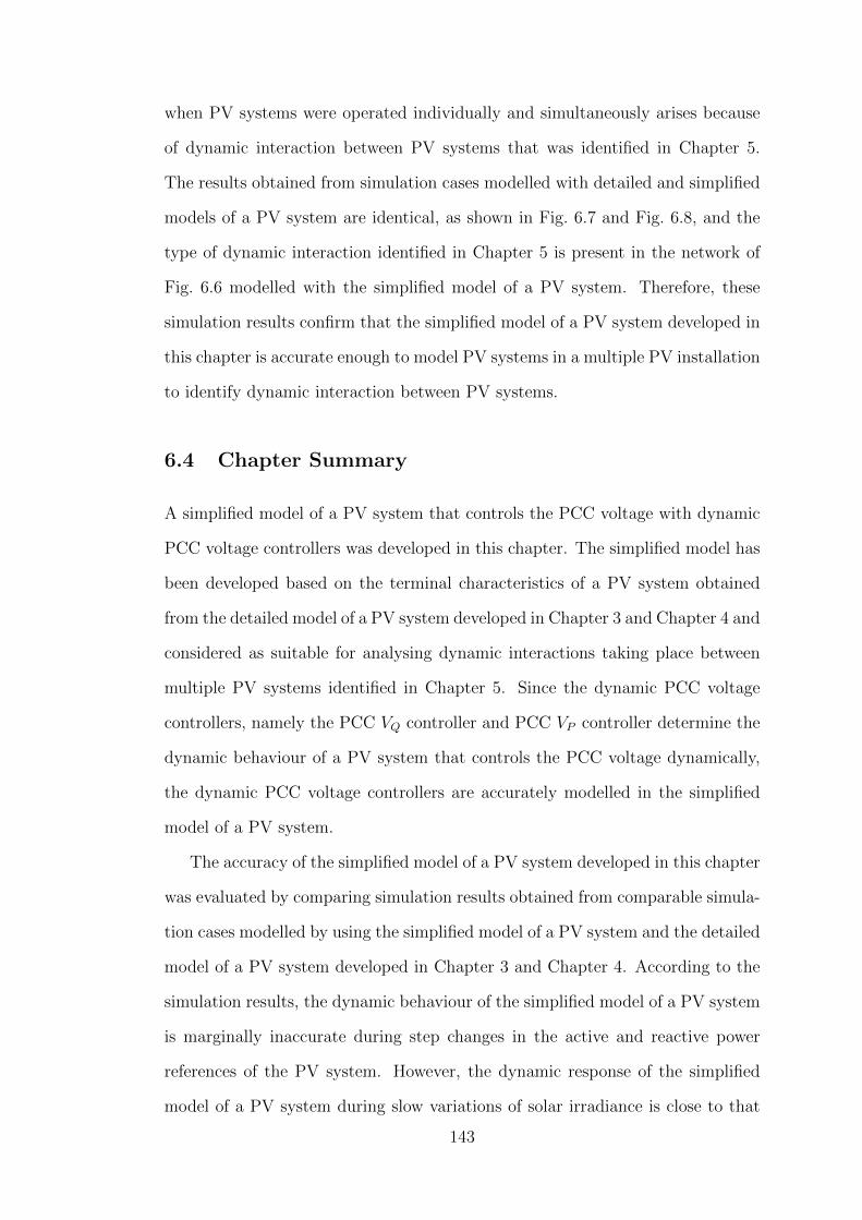
when PV systems were operated individually and simultaneously arises because
of dynamic interaction between PV systems that was identified in Chapter 5.
The results obtained from simulation cases modelled with detailed and simplified
models of a PV system are identical, as shown in Fig. 6.7 and Fig. 6.8, and the
type of dynamic interaction identified in Chapter 5 is present in the network of
Fig. 6.6 modelled with the simplified model of a PV system. Therefore, these
simulation results confirm that the simplified model of a PV system developed in
this chapter is accurate enough to model PV systems in a multiple PV installation
to identify dynamic interaction between PV systems.
6.4 Chapter Summary
A simplified model of a PV system that controls the PCC voltage with dynamic
PCC voltage controllers was developed in this chapter. The simplified model has
been developed based on the terminal characteristics of a PV system obtained
from the detailed model of a PV system developed in Chapter 3 and Chapter 4 and
considered as suitable for analysing dynamic interactions taking place between
multiple PV systems identified in Chapter 5. Since the dynamic PCC voltage
controllers, namely the PCC VQ controller and PCC VP controller determine the
dynamic behaviour of a PV system that controls the PCC voltage dynamically,
the dynamic PCC voltage controllers are accurately modelled in the simplified
model of a PV system.
The accuracy of the simplified model of a PV system developed in this chapter
was evaluated by comparing simulation results obtained from comparable simula-
tion cases modelled by using the simplified model of a PV system and the detailed
model of a PV system developed in Chapter 3 and Chapter 4. According to the
simulation results, the dynamic behaviour of the simplified model of a PV system
is marginally inaccurate during step changes in the active and reactive power
references of the PV system. However, the dynamic response of the simplified
model of a PV system during slow variations of solar irradiance is close to that
143
predicted by the detailed model. Further, though the dynamic characteristics of
the PCC VQ controller has been modelled accurately in the simplified model of
a PV system, the transient behaviour of the PCC VP controller in the simplified
model of a PV system is slightly different to that of the detailed model of a PV
system. The inaccuracy in the transient characteristics of the PCC VQ controller
in the simplified model of a PV system arises because of the absence of non-linear
characteristics of a PV array in that model.
The dynamic behaviour of inner control loops, the total control system of a
PV system and MPPT algorithm are disregarded while developing the simplified
model. Therefore, the simplified model of a PV system developed in this chapter
may not be an accurate representation of an actual PV system for certain simu-
lation studies. Hence the appropriateness of using the simplified model of a PV
system in simulation studies should be evaluated before using this model.
The simulation results presented in this chapter confirm that the developed
simplified model of a PV system is a sufficiently accurate model of a grid-connected
PV system that controls the PCC voltage with dynamic PCC voltage controllers.
Further, simulation studies have confirmed that a simulation case modelled with
the simplified model of a PV system can be performed 15 times faster than a
comparable simulation case that is modelled with the detailed model of a PV
system. In this chapter, the operation of only one or two grid-connected PV
systems were considered to demonstrate the accuracy of the developed simplified
model of a PV system. The accuracy of the simplified model of a PV system
to represent PV systems in an installation of more than two PV systems will
be confirmed in Chapter 7 of this Thesis. Therefore, in order to model an LV
power grid integrated with multiple PV systems to identify dynamic interaction
between PV systems that control respective PCC voltage with dynamic PCC
voltage controllers and to obtain simulation results within a short period of time,
the simplified model of a PV system can be used.
144
Chapter 7
Power sharing between multiple
solar PV systems in a radial
distribution feeder
7.1 Introduction
In a grid to which multiple solar PV systems are integrated, network voltage
rise has been identified in Chapter 2 as a critical technical matter that should be
addressed. In such a grid, voltage may rise to considerably higher levels, especially
during the day time when power generation from PV systems is at the highest
level and load on the grid is at a minimum. The standards applicable to grid-
integrated PV systems impose a maximum voltage level below which PV systems
may stay connected to the grid. The Australian standard that is applicable to
grid-integrated PV systems is AS4777.2 [7]. As per [7], the highest grid voltage
that PV systems may stay connected is 230 V + 10% (herein after referred to as
Umax). If the PCC voltage of a PV system exceeds Umax, after a defined time
period the PV system should disconnect from the grid that leads to a loss of
potential revenue to the owner of the PV system and loss of generation.
The voltage at the PCC of a PV system is a function of both the grid
impedance and real and reactive power injected. Therefore, in certain operat-
145
ing situations, the voltage at the PCC of a PV system where voltage sensitivity
is high may exceed Umax while the PCC voltages of other PV systems connected
to the grid are below Umax. In such a situation the PV system that is connected
to the grid at a node where voltage sensitivity is high may disconnect in order
to comply within the Australian standard AS477.2 [7] while other PV systems
will continue to operate. This scenario highlights that in certain operating sit-
uations, owners of PV systems whose PV systems are integrated to the grid at
nodes where voltage sensitivity is high are disadvantaged over the other PV sys-
tem owners whose PV systems are connected to the grid at nodes where voltage
sensitivity is less. Therefore, in this chapter a power sharing methodology is de-
veloped for PV systems that are integrated to a radial distribution feeder. The
developed methodology will minimise the disadvantages associated with the volt-
age sensitivity at the PCC of a PV system that an owner of a grid-integrated PV
system may experience.
In the power sharing method proposed in this chapter, a voltage bandwidth
is determined for each PV system connected to a radial distribution feeder. Since
the voltage bandwidth of a PV system is determined based on the voltage sensitiv-
ity at the PCC of the PV system, power sharing between PV systems connected
to the radial distribution feeder is achieved. In the proposed method, closed-loop
PCC voltage controllers developed in Chapter 4 are used to ensure that the PCC
voltage of each PV system is maintained within the allocated bandwidth while
sharing active power. Further, the use of closed-loop PCC voltage controllers
in PV systems guarantee that the voltage of the radial distribution feeder at no
location exceeds Umax.
7.2 Model of a power distribution feeder
A single-phase power distribution feeder to which five PV systems are connected
is considered in order to develop the power sharing methodology. The model
of the distribution feeder is shown in Fig. 7.1. The power grid is modelled as
146

XR
Vs
Infinite grid
XR XR XR XR
PV1
N1 N2 N3 N4 N5
PV2 PV3 PV4 PV5
N0
Figure 7.1: Model of a power distribution feeder
an equivalent Thevenin voltage source with an rms voltage Vs = 240 V. The
impedances of high and medium voltage power lines and transformers are assumed
to be negligible compared to that of the distribution feeder. Hence, the equivalent
impedance of the grid is the impedance of the distribution transformer. The
impedance of the the distribution transformer is 4%1 and is incorporated with
the feeder impedance.
The distribution feeder is modelled with five equally spaced line sections. Each
line section has a resistance, R, and a reactance, X. The PV systems are assumed
as directly connected to the distribution feeder without a service wire since the
impedance of a service wire is generally small. The reference impedance for low
voltage public supply systems that is given in [62] for electrical apparatus testing
purposes is considered as the grid impedance seen by the PV system PV5 located
at the end of the distribution feeder. Hence the grid impedance seen by PV5 is
(0.4 + j0.25) Ω.
The distribution feeder is connected with five PV systems that are equally
spaced along the feeder. Since the PV systems are equally spaced and the
impedance of the distribution transformer is considered equally distributed along
the feeder, R = 0.08 Ω and X = j0.05 Ω. PV systems PV1 − PV5 are con-
nected at nodes N1 −N5 respectively. Nodes N1 −N5 are the points of common
coupling (PCC) of the PV systems. The rated capacity of each PV array is 5 kW.
The PV systems are integrated to the grid via VSCs. The rated capacity of each
1This is equivalent to the impedance of a typical 300 kVA low voltage power distributiontransformer.
147
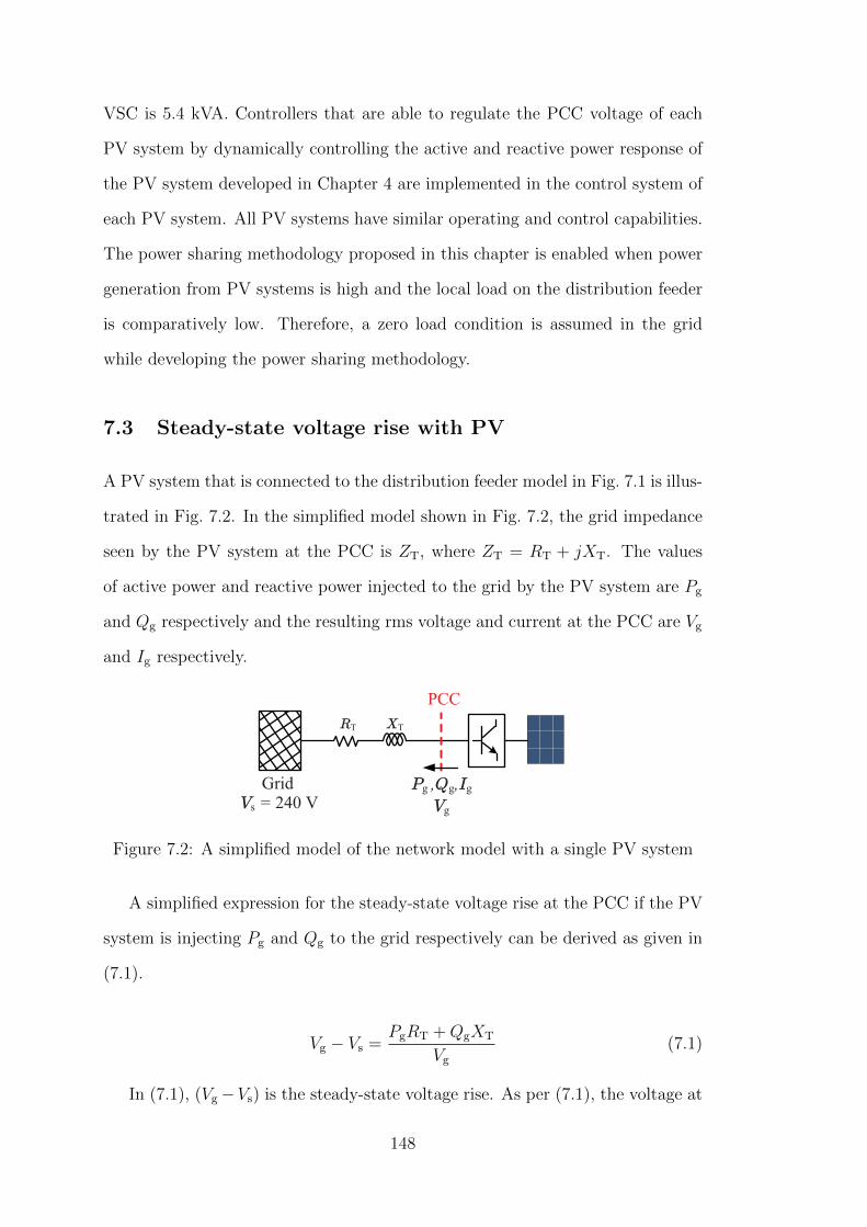
VSC is 5.4 kVA. Controllers that are able to regulate the PCC voltage of each
PV system by dynamically controlling the active and reactive power response of
the PV system developed in Chapter 4 are implemented in the control system of
each PV system. All PV systems have similar operating and control capabilities.
The power sharing methodology proposed in this chapter is enabled when power
generation from PV systems is high and the local load on the distribution feeder
is comparatively low. Therefore, a zero load condition is assumed in the grid
while developing the power sharing methodology.
7.3 Steady-state voltage rise with PV
A PV system that is connected to the distribution feeder model in Fig. 7.1 is illus-
trated in Fig. 7.2. In the simplified model shown in Fig. 7.2, the grid impedance
seen by the PV system at the PCC is ZT, where ZT = RT + jXT. The values
of active power and reactive power injected to the grid by the PV system are Pg
and Qg respectively and the resulting rms voltage and current at the PCC are Vg
and Ig respectively.
RT
Vs = 240 VGrid
PCC
Pg ,Qg,Ig
Vg
XT
Figure 7.2: A simplified model of the network model with a single PV system
A simplified expression for the steady-state voltage rise at the PCC if the PV
system is injecting Pg and Qg to the grid respectively can be derived as given in
(7.1).
Vg − Vs =PgRT +QgXT
Vg
(7.1)
In (7.1), (Vg−Vs) is the steady-state voltage rise. As per (7.1), the voltage at
148

the PCC is increased if active power is injected to the grid by the PV system and
if reactive power is absorbed by the PV system, the PCC voltage can be reduced.
7.4 Determining a reference PCC voltage for each PV
system to share active power
The reference PCC voltage of each PV system determines the setting above which
the dynamic PCC voltage controllers are activated. The reference PCC voltage
for each PV system is derived initially in such a way that if power curtailing
is required to keep the network voltage within limits. Once power curtailing is
done to bring the network voltage within limits, each PV system injects an equal
amount of power to the grid irrespective of the point of connection of each PV
system. In this section, the methodology that is used to determine the reference
PCC voltage of each PV system is described in detail with reference to the model
of a power distribution feeder shown in Fig. 7.1. In this section, PV systems are
assumed to have no reactive power injection or absorption capabilities.
In the power distribution model shown in Fig. 7.1, the voltage rise at each
node with respect to the immediately following node (towards the grid) can be
found by using (7.1) at steady-state. Equation (7.1) is written as in (7.2) with
different notations in order to mathematically represent the steady-state voltage
rise in each node of the network model shown in Fig. 7.1. In (7.2), Vn is the
voltage at the node Nn (n = 1, 2, .., 5) that is of interest to determine the steady-
state voltage rise, Vn−1 is the voltage at the node Nn−1, Pn and Qn are the total
active and reactive power that flows to the grid through the node Nn respectively,
and R and X are the resistance and the reactance of the line section Nn−Nn−1.
Vn − Vn−1 =PnR +QnX
Vn(7.2)
In order to find the steady-state voltage rise at node Nn (n = 1, 2, .., 5) with
respect to node Nn−1 by using (7.2) the voltage at node Nn−1 and the power
149
that flows through node Nn should be known. Since the voltage at a node is a
function of the active and reactive power injected by the PV system connected
at that particular node as well as by other PV systems connected to the feeder,
the voltage at each node can be found only by an iterative process. The iterative
method that is used to determine the reference PCC voltage of each PV system
is described here.
The active power injected by each PV system is assumed to be equal in each
iteration. The network losses are disregarded. Since network losses are disre-
garded and a no-load condition is assumed, the active power that flows through a
node is the summation of the active power injected by the PV system connected
to the particular node and active power injected by all other PV systems that
are connected to the distribution feeder downstream of the node of interest. If
the active power injected by each PV system is P , then the active power flows
to the grid at node Nn is (6− n)P since the total number of PV systems in the
network model in Fig. 7.1 is five.
The voltage at the node Nn when the active power flowing through the node
to the grid is P and the reactive power flowing through the node is zero, can be
found by solving (7.2) for Vn. The resulting equation is given in (7.3) that is used
to iteratively determine the reference PCC voltage of each PV system to ensure
equal share of active power.
Vn =Vn−1 +
√V 2n−1 + 4(6− n)PR
2(n=1,2,..,5) (7.3)
The active power injected by each PV system is set at the beginning of an
iteration. Since the voltage at the node N0 is 240 V, voltages at following nodes
can be found by (7.3) when the power injected by each PV system is known.
Since the voltage sensitivity of the node N5 in the network model is higher than
all other nodes, the voltage at N5 reaches the maximum voltage limit, Umax, first.
Therefore, after finding voltages at all the nodes in an iteration, the voltage at
node N5, V5, is compared with Umax. If V5 ≤ Umax then node voltages calculated
150

in the current iteration are stored, the active power injected by each PV system
that is set at the beginning of the current iteration is incremented and the next
iteration is commenced. If V5 > Umax, the node voltages calculated at the previous
iteration are considered as the reference PCC voltage of the respective PV system.
The reference PCC voltages that are calculated by the described iterative
process for the network model shown in Fig. 7.1 are given in Table 7.1. According
to the results obtained using the iterative method, each PV system should inject
2.69 kW of active power to the grid if the respective PCC voltage is regulated by
curtailing active power at the reference PCC voltage given in Table 7.1.
Table 7.1: Reference PCC voltages for PV systems to share active power equally
PV system (PVn) Reference PCC voltage (V)
PV1 244.4
PV2 247.8
PV3 250.4
PV4 252.1
PV5 253.0
7.5 Simulation results - Part A
The network model shown in Fig. 7.1 was simulated in the PSCAD/EMTDC
simulation program. Each PV system was modelled by using the simulation
model of a grid-connected PV system developed in Chapter 3. Furthermore,
the dynamic PCC voltage controller that is able to regulate the PCC voltage of
a PV system by controlling active power response of the PV system developed
in Chapter 4 was integrated within the simulation models of PV systems. The
reference voltage of the PCC voltage controller in each respective PV system was
set using the voltages references given in Table 7.1. The solar irradiance level
at each PV system was 1200 W/m2 and the surface temperature of all the PV
arrays were considered constant at 30 C.
At the beginning of the simulation, all PV systems were operating at the
151

maximum power point and the PCC voltage controllers were inactive. At time
t = 1 s, PCC voltage controllers were activated in all PV systems. The simulation
was run for 20 s. The voltage variations at all five nodes that are connected with
PV systems and the active power variation at each PV system are illustrated in
Fig. 7.3. As shown in Fig. 7.3(a), once the controllers were activated, the PCC
voltage at each PV system is regulated at the respective reference PCC voltage.
The voltage profile of the network is shown in Fig. 7.4 before and after the PCC
voltage controllers were activated.
2 4 6 8 10 12 14 16 18 20−5
−4
−3
−2
(b)Time (s)
ActivePower
(kW)
Variation of active power injected to grid by each PV system
2 4 6 8 10 12 14 16 18 20240
245
250
255
260
265
(a)
RMSVoltage(V
)
Voltage variation at nodes
V5 V4 V3
V2 V1
PPV5
PPV1
PPV2
PPV3
PPV4
Figure 7.3: Simulation results - Part A - PCC voltage and active power variationof PV systems
The amount of active power injected by each PV system before controllers
were activated and after power was curtailed to regulate the respective PCC
voltage is shown in Fig. 7.5. Initially, each PV system was injecting about 4.85 kW
of active power to the grid. Once active power was curtailed to regulate the PCC
voltage and controllers reached steady-state, each of the PV systems was injecting
about 2.69 kW of active power to the grid. This is the expected amount of active
power injection by each PV system if the respective PCC voltage is regulated
at the reference voltage given in Table 7.1. As per Fig. 7.5, there are slight
152
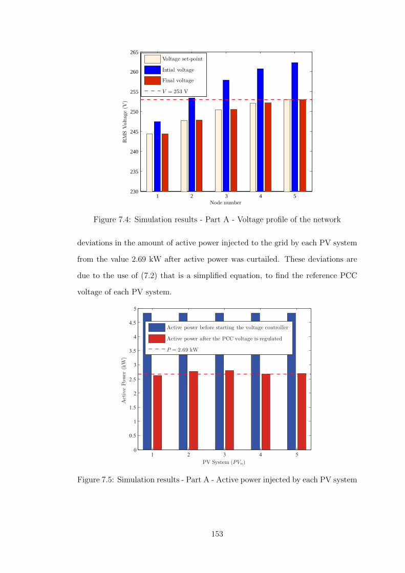
1 2 3 4 5230
235
240
245
250
255
260
265
Node number
RMSVoltage(V
)
Voltage set-point
Intial voltage
Final voltage
V = 253 V
Figure 7.4: Simulation results - Part A - Voltage profile of the network
deviations in the amount of active power injected to the grid by each PV system
from the value 2.69 kW after active power was curtailed. These deviations are
due to the use of (7.2) that is a simplified equation, to find the reference PCC
voltage of each PV system.
1 2 3 4 50
0.5
1
1.5
2
2.5
3
3.5
4
4.5
5
PV System (PVn)
ActivePower
(kW)
Active power before starting the voltage controller
Active power after the PCC voltage is regulated
P = 2.69 kW
Figure 7.5: Simulation results - Part A - Active power injected by each PV system
153
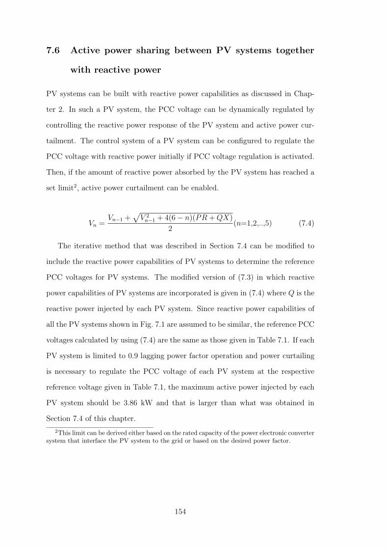
7.6 Active power sharing between PV systems together
with reactive power
PV systems can be built with reactive power capabilities as discussed in Chap-
ter 2. In such a PV system, the PCC voltage can be dynamically regulated by
controlling the reactive power response of the PV system and active power cur-
tailment. The control system of a PV system can be configured to regulate the
PCC voltage with reactive power initially if PCC voltage regulation is activated.
Then, if the amount of reactive power absorbed by the PV system has reached a
set limit2, active power curtailment can be enabled.
Vn =Vn−1 +
√V 2n−1 + 4(6− n)(PR +QX)
2(n=1,2,..,5) (7.4)
The iterative method that was described in Section 7.4 can be modified to
include the reactive power capabilities of PV systems to determine the reference
PCC voltages for PV systems. The modified version of (7.3) in which reactive
power capabilities of PV systems are incorporated is given in (7.4) where Q is the
reactive power injected by each PV system. Since reactive power capabilities of
all the PV systems shown in Fig. 7.1 are assumed to be similar, the reference PCC
voltages calculated by using (7.4) are the same as those given in Table 7.1. If each
PV system is limited to 0.9 lagging power factor operation and power curtailing
is necessary to regulate the PCC voltage of each PV system at the respective
reference voltage given in Table 7.1, the maximum active power injected by each
PV system should be 3.86 kW and that is larger than what was obtained in
Section 7.4 of this chapter.
2This limit can be derived either based on the rated capacity of the power electronic convertersystem that interface the PV system to the grid or based on the desired power factor.
154

7.7 Simulation results - Part B
The dynamic PCC voltage controller that regulate the PCC voltage by control-
ling the reactive power response of a PV system and developed in Chapter 4
is integrated with each PV system in the simulation model used in Section 7.5.
The control system of each PV system is configured to utilise the reactive power
capabilities of each PV system initially if PCC voltage regulation is necessary.
The minimum lagging power factor of each PV system is set as 0.9. Once a PV
system reaches the maximum reactive power limit, the respective controller is sat-
urated and active power curtailing is enabled to regulate the PCC voltage. The
minimum lagging power factor of a PV system is still maintained when power is
curtailed to regulate the PCC voltage.
In order to demonstrate the robustness of the power sharing methodology
presented in this chapter, a dynamically varying solar irradiance level was applied
to the simulation model. The considered variation of solar irradiance at each PV
system is illustrated in Fig. 7.6 and respective dynamic variations of PCC voltage,
active and reactive power are shown in Fig. 7.7. The latter figure illustrates that
PCC voltage regulation in each PV system is initially achieved by absorbing
reactive power from the grid. Once the reactive power limit of each PV system
is reached, active power has been curtailed to regulate the PCC voltage.
5 10 15 20 25 300
500
1000
Time (s)
SolarIrradiance
(W/m
2)
PV2 and PV4
PV1 , PV3 and PV5
Figure 7.6: Variation of solar irradiance
The dynamic performance of the simplified model of a PV system developed
in Chapter 6 of this Thesis was validated in Section 6.3 using simulation case
studies that consisted of only one or two grid-connected PV systems. In order to
155

5 10 15 20 25 30240
245
250
255
260
(a)
RMSVoltage(V
)
Voltage variation at nodes
5 10 15 20 25 30
−5
−4
−3
−2
−1
0
(c)Time (s)
ActivePower
(kW)
Variation of active power injected to the grid by each PV system
5 10 15 20 25 30−3
−2
−1
0
1Variation of reactive power injected to the grid by each PV system
(b)
ReactivePower
(kVAr)
V5V3
V2 V1
V4V = 253 V
QPV2
QPV4 QPV3
QPV5
QPV1
PPV3
PPV5
PPV1
PPV4
PPV2
Figure 7.7: Simulation results - Part B - PCC voltage and active and reactivepower variation of PV systems
156

5 10 15 20 25 30
−5
−4
−3
−2
−1
0
(c)Time (s)
Activepower
(kW)
Variation of active power injected to the grid by each PV system
5 10 15 20 25 30−3
−2
−1
0
1Variation of reactive power absorbed by each PV system
(b)
Reactivepower
(kVAr)
5 10 15 20 25 30240
245
250
255
260
(a)
Voltage(V
)
Voltage variation at nodes
V5V3
V2 V1
V4V = 253 V
QPV2
QPV4
QPV1
QPV5 QPV3
PPV3PPV4
PPV5
PPV2
PPV1
Figure 7.8: Simulation results - Part B - PCC voltage and active and reactivepower variation of PV systems modelled by using the simplified model of a PVsystem
157
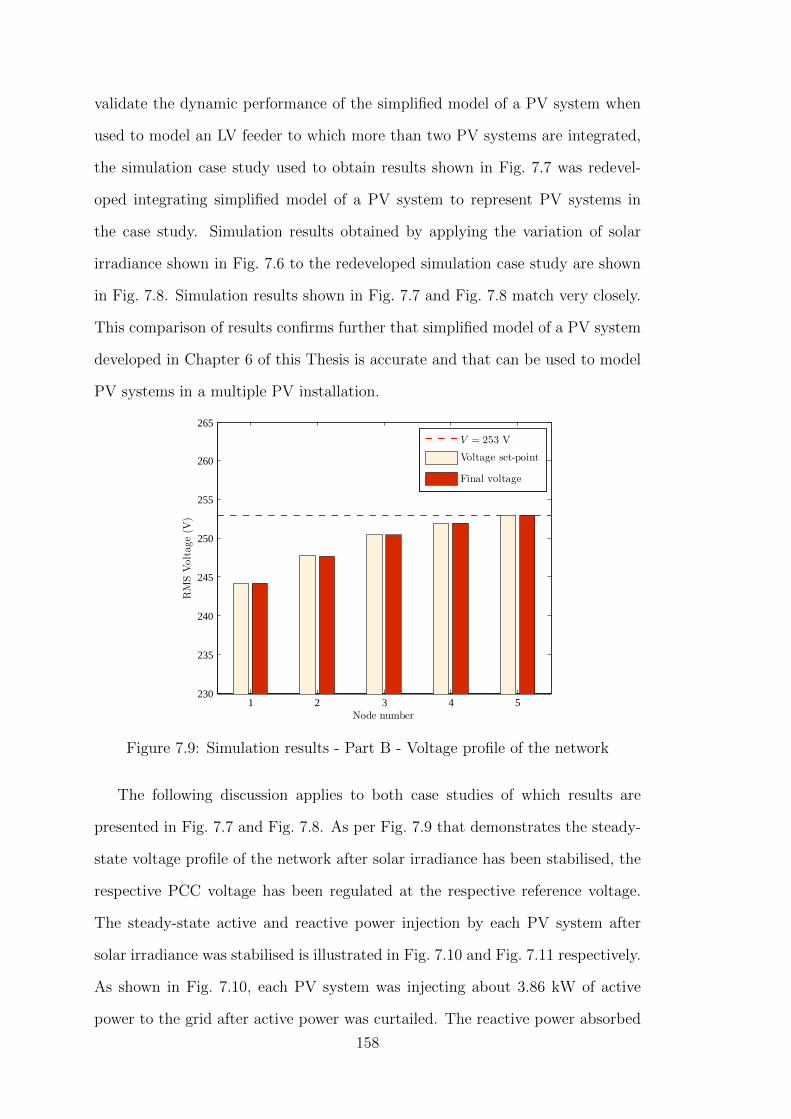
validate the dynamic performance of the simplified model of a PV system when
used to model an LV feeder to which more than two PV systems are integrated,
the simulation case study used to obtain results shown in Fig. 7.7 was redevel-
oped integrating simplified model of a PV system to represent PV systems in
the case study. Simulation results obtained by applying the variation of solar
irradiance shown in Fig. 7.6 to the redeveloped simulation case study are shown
in Fig. 7.8. Simulation results shown in Fig. 7.7 and Fig. 7.8 match very closely.
This comparison of results confirms further that simplified model of a PV system
developed in Chapter 6 of this Thesis is accurate and that can be used to model
PV systems in a multiple PV installation.
1 2 3 4 5230
235
240
245
250
255
260
265
Node number
RMSVoltage(V
)
V = 253 V
Voltage set-point
Final voltage
Figure 7.9: Simulation results - Part B - Voltage profile of the network
The following discussion applies to both case studies of which results are
presented in Fig. 7.7 and Fig. 7.8. As per Fig. 7.9 that demonstrates the steady-
state voltage profile of the network after solar irradiance has been stabilised, the
respective PCC voltage has been regulated at the respective reference voltage.
The steady-state active and reactive power injection by each PV system after
solar irradiance was stabilised is illustrated in Fig. 7.10 and Fig. 7.11 respectively.
As shown in Fig. 7.10, each PV system was injecting about 3.86 kW of active
power to the grid after active power was curtailed. The reactive power absorbed
158

1 2 3 4 50
0.5
1
1.5
2
2.5
3
3.5
4
4.5
5
PV System (PVn)
ActivePower
(kW) P = 3.86 kW
Active power before the variation of solar irradiance
Active power after the solar irradiance is stabilised
Figure 7.10: Simulation results - Part B - Active power injected by each PVsystem
1 2 3 4 50
0.5
1
1.5
2
2.5
PV System (PVn)
ReactivePower
(kVAr)
Q= 1.87 kVAr
Reactive power absorbed by each PV system
Figure 7.11: Simulation results - Part B - Reactive power absorbed by each PVsystem
by each PV system has been limited to 0.9 lagging power factor operation of the
PV system as illustrated in Fig. 7.11. Simulation results presented in this section
demonstrate that by operating each PV system of the network at the respective
reference PCC voltage given in Table 7.1, active power sharing can be achieved
in the network shown in Fig. 7.1.
159

7.8 Experimental results
The power sharing methodology proposed for PV systems connected to a ra-
dial power distribution feeder in this chapter was experimentally validated. The
experimental setup that was used to obtain experimental results presented in
Chapter 5 of this Thesis was used to validate the power sharing methodology
developed in this chapter.
Grid
X01R01N1 N2
PV1 PV2
N0
Iq1 Iq2
X12R12
Figure 7.12: Schematic diagram of the experimental setup
A schematic diagram of the experimental setup used is shown in Fig. 7.12.
In the experimental setup, (R01 + jX01) = (0.25 + j0.25) Ω and (R12 + jX12) =
(0.12 + j0.08) Ω with reference to Fig. 7.12 and the grid voltage was set as
251 V. The reference voltages of PCC voltage controllers of PV1 and PV2 were
set as 252.2√
2 V and 253√
2 V respectively and those values were determined
by applying the iterative method described in Section 7.4 of this chapter to the
network model of the experimental setup shown in Fig. 7.12. A Hioki 3196 power
quality analyser was used to record active and reactive power injected by PV
systems and PCC voltages of PV systems.
The experimental results obtained when PCC voltage control was done only by
curtailing active power is shown in Fig. 7.13. In this experiment, reactive power
controllers of PV systems were inactive. The step changes that can be seen in
Fig. 7.13 are due to 400 W/m2 to 1000 W/m2 step changes of solar irradiance
levels simulated in the experimental setup.
Fig. 7.13 illustrates that when solar irradiance level was 400 W/m2 both PV
160
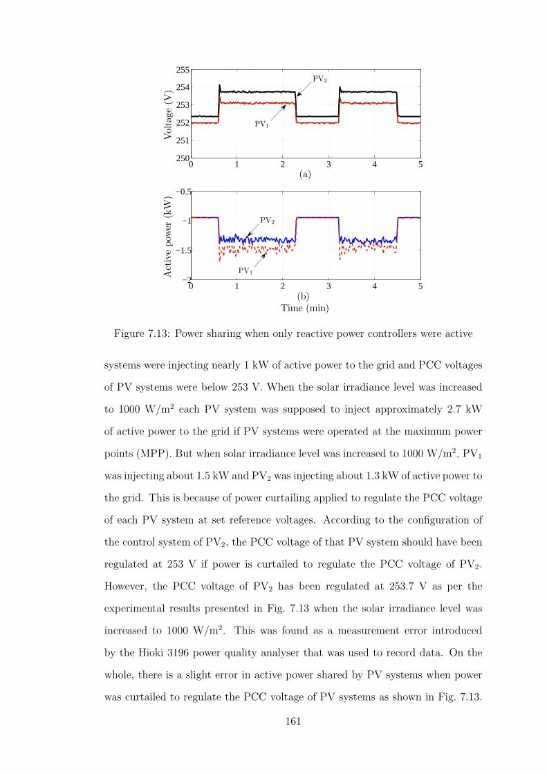
0 1 2 3 4 5250
251
252
253
254
255
Voltage
(V)
(a)
0 1 2 3 4 5−2
−1.5
−1
−0.5
Activepow
er(kW
)
(b)Time (min)
PV1
PV2
PV2
PV1
Figure 7.13: Power sharing when only reactive power controllers were active
systems were injecting nearly 1 kW of active power to the grid and PCC voltages
of PV systems were below 253 V. When the solar irradiance level was increased
to 1000 W/m2 each PV system was supposed to inject approximately 2.7 kW
of active power to the grid if PV systems were operated at the maximum power
points (MPP). But when solar irradiance level was increased to 1000 W/m2, PV1
was injecting about 1.5 kW and PV2 was injecting about 1.3 kW of active power to
the grid. This is because of power curtailing applied to regulate the PCC voltage
of each PV system at set reference voltages. According to the configuration of
the control system of PV2, the PCC voltage of that PV system should have been
regulated at 253 V if power is curtailed to regulate the PCC voltage of PV2.
However, the PCC voltage of PV2 has been regulated at 253.7 V as per the
experimental results presented in Fig. 7.13 when the solar irradiance level was
increased to 1000 W/m2. This was found as a measurement error introduced
by the Hioki 3196 power quality analyser that was used to record data. On the
whole, there is a slight error in active power shared by PV systems when power
was curtailed to regulate the PCC voltage of PV systems as shown in Fig. 7.13.
161
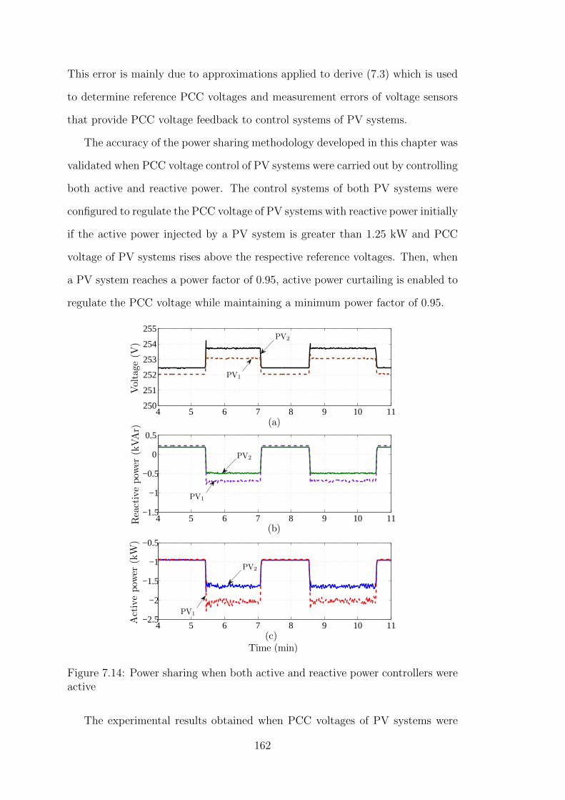
This error is mainly due to approximations applied to derive (7.3) which is used
to determine reference PCC voltages and measurement errors of voltage sensors
that provide PCC voltage feedback to control systems of PV systems.
The accuracy of the power sharing methodology developed in this chapter was
validated when PCC voltage control of PV systems were carried out by controlling
both active and reactive power. The control systems of both PV systems were
configured to regulate the PCC voltage of PV systems with reactive power initially
if the active power injected by a PV system is greater than 1.25 kW and PCC
voltage of PV systems rises above the respective reference voltages. Then, when
a PV system reaches a power factor of 0.95, active power curtailing is enabled to
regulate the PCC voltage while maintaining a minimum power factor of 0.95.
4 5 6 7 8 9 10 11250
251
252
253
254
255
Voltage
(V)
(a)
4 5 6 7 8 9 10 11−1.5
−1
−0.5
0
0.5
Reactivepow
er(kVAr)
(b)
4 5 6 7 8 9 10 11−2.5
−2
−1.5
−1
−0.5
Activepow
er(kW
)
(c)Time (min)
PV1
PV1
PV1
PV2
PV2
PV2
Figure 7.14: Power sharing when both active and reactive power controllers wereactive
The experimental results obtained when PCC voltages of PV systems were
162

regulated by controlling both active and reactive power are shown in Fig. 7.14.
Similar to Fig. 7.13, the step changes that can be seen in Fig. 7.14 are due to
400 W/m2 to 1000 W/m2 step changes in solar irradiance levels simulated in the
experimental setup.
Fig. 7.14 illustrates that when the solar irradiance level was 400 W/m2 both
PV systems were injecting about 1 kW of active power and no reactive power
to the grid. When solar irradiance level was increased to 1000 W/m2, PV1 was
injecting about 2 kW of active power while absorbing about 0.7 kVAr of reac-
tive power from the grid and PV2 was injecting about 1.6 kW of active power
while absorbing about 0.5 kVAr of reactive power from the grid. The exper-
imental results presented in Fig. 7.14 confirm that when solar irradiance level
was increased to 1000 W/m2, active power was curtailed by each PV system to
regulate the PCC voltage since expected active power output of each PV system
was about 2.7 kW. Further, PV systems have operated at 0.95 power factor when
solar irradiance level was increased to 1000 W/m2 and that confirms the regu-
lation of PCC voltage of each PV system with reactive power before curtailing
active power. As expected, active power injection by PV systems has increased in
this experiment compared to the experimental results shown in Fig. 7.13. On the
whole, the experimental results presented in Fig. 7.14 confirm that power sharing
methodology developed for PV systems that control PCC voltages by controlling
both active and reactive power, is acceptable and accurate enough despite the
fact there were slight errors introduced by PCC voltage sensors of PV systems.
7.9 Discussion
The power sharing methodologies proposed in the current research have been
successfully applied to the network shown in Fig. 7.1 in a simulation study. Ac-
cording to simulation results obtained, there are minor deviations in the amount
of active power shared between PV systems from what is expected as shown in
Fig. 7.5 and Fig. 7.10. These deviations are mainly due to the use of (7.3) or (7.4)
163

that are simplified expressions, based on assumptions to determine the reference
PCC voltages for each PV system as given in Table 7.1. The stated deviations
in active power shared by each PV system can be further minimised if reference
PCC voltages are determined through a detailed load flow analysis of the network
shown in Fig. 7.1.
In the network model shown in Fig. 7.1, upstream impedances are disregarded
and the impedance of the distribution transformer is assumed as equally dis-
tributed along the distribution feeder. However, in a practical situation, there
are upstream impedances and the impedance of the distribution transformer is
a lumped impedance. Although the assumption is a significant deviation from a
real situation, it does not introduce any inaccuracy to the developed power shar-
ing methodology if it is implemented in an actual power system. This is because,
in an actual power system, the upstream or downstream power flow through the
distribution transformer causes the voltage to change in the whole distribution
feeder equally.
The reference PCC voltages given in Table 7.1 are applicable only to the net-
work shown in Fig. 7.1. If an additional PV system is integrated to the network,
reference PCC voltages should be recalculated to suit the new network. If the
developed power sharing methodology is practically implemented in a radial dis-
tribution feeder, since PV systems are being integrated to the grid continuously,
there will be a need to change in the reference PCC voltage level of each PV
system connected to the considered feeder when an additional PV system is in-
tegrated. Such a requirement can be minimised by zoning the feeder as shown
in Fig. 7.15 and allocating a voltage reference for a particular zone. In this ap-
proach, all PV systems connected to a particular zone of a feeder will have the
same PCC voltage reference.
The power sharing methodology developed in this chapter was applied to a
power distribution feeder that was divided into three zones as shown in Fig. 7.15.
In order to determine the reference PCC voltages of PV systems connected at
164
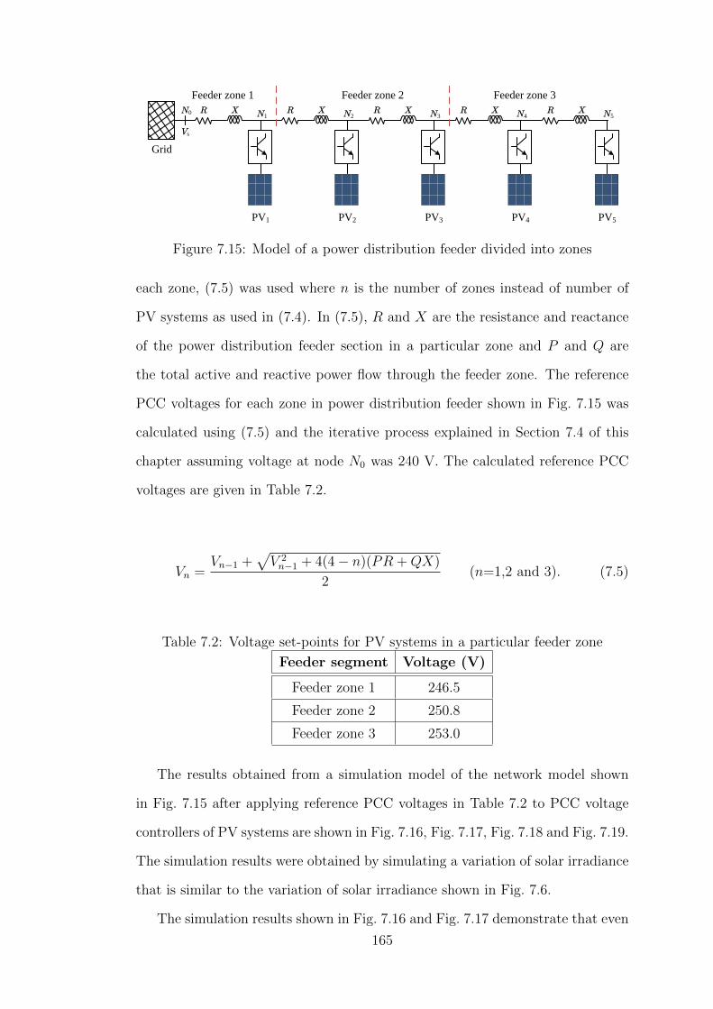
XR
Grid
XR XR XR XR
PV1
N1 N2 N3 N4 N5
PV2 PV3 PV4 PV5
Feeder zone 1 Feeder zone 2 Feeder zone 3
Vs
N0
Figure 7.15: Model of a power distribution feeder divided into zones
each zone, (7.5) was used where n is the number of zones instead of number of
PV systems as used in (7.4). In (7.5), R and X are the resistance and reactance
of the power distribution feeder section in a particular zone and P and Q are
the total active and reactive power flow through the feeder zone. The reference
PCC voltages for each zone in power distribution feeder shown in Fig. 7.15 was
calculated using (7.5) and the iterative process explained in Section 7.4 of this
chapter assuming voltage at node N0 was 240 V. The calculated reference PCC
voltages are given in Table 7.2.
Vn =Vn−1 +
√V 2n−1 + 4(4− n)(PR +QX)
2(n=1,2 and 3). (7.5)
Table 7.2: Voltage set-points for PV systems in a particular feeder zone
Feeder segment Voltage (V)
Feeder zone 1 246.5
Feeder zone 2 250.8
Feeder zone 3 253.0
The results obtained from a simulation model of the network model shown
in Fig. 7.15 after applying reference PCC voltages in Table 7.2 to PCC voltage
controllers of PV systems are shown in Fig. 7.16, Fig. 7.17, Fig. 7.18 and Fig. 7.19.
The simulation results were obtained by simulating a variation of solar irradiance
that is similar to the variation of solar irradiance shown in Fig. 7.6.
The simulation results shown in Fig. 7.16 and Fig. 7.17 demonstrate that even
165
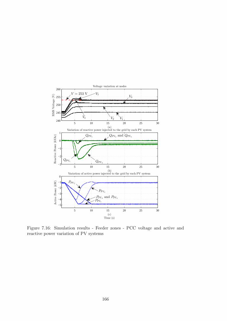
5 10 15 20 25 30240
245
250
255
260
(a)
RMSVoltage(V
)
Voltage variation at nodes
5 10 15 20 25 30
−5
−4
−3
−2
−1
0
(c)Time (s)
ActivePower
(kW)
Variation of active power injected to the grid by each PV system
5 10 15 20 25 30−3
−2
−1
0
1Variation of reactive power injected to the grid by each PV system
(b)
ReactivePower
(kVAr)
V1V2
V3V5
V4
V = 253 V
PPV5
PPV3
PPV1
PPV2 and PPV4
QPV5 QPV3
QPV2 and QPV4QPV1
Figure 7.16: Simulation results - Feeder zones - PCC voltage and active andreactive power variation of PV systems
166

1 2 3 4 5230
235
240
245
250
255
260
265
Node number
RMSVoltage(V
)
Voltage set-point
Final Voltage
V = 253 V
Figure 7.17: Simulation results - Feeder zones - Voltage profile of the network
1 2 3 4 50
0.1
0.2
0.3
0.4
0.5
PV System (PVn)
ReactivePower
(kVAr)
Reactive power absorbed by each PV System
Figure 7.18: Simulation results - Feeder zones - Reactive power absorbed by eachPV system
though the power distribution feeder was divided into zones, the voltage along
the feeder has been maintained below 253 V at times when the voltage levels
of the feeder was likely to exceed 253 V. Fig. 7.18 and Fig. 7.19 demonstrate
that though the feeder voltage was maintained below 253 V, the accuracy of the
power sharing methodology developed in this chapter has been compromised after
167

1 2 3 4 50
0.5
1
1.5
2
2.5
3
3.5
4
4.5
5
PV System (PVn)
ActivePower
(kW) Maximum active power could be injected by PV systems
Active power injected by PV systems
Figure 7.19: Simulation results - Feeder zones - Active power injected by eachPV system
applying reference PCC voltages derived based on feeder zones shown in Fig. 7.15.
On the whole, these simulation results confirm that zoning a power distribution
feeder may minimise the need for frequent adjustment of control parameters of
PV systems connected to a power distribution feeder to share active and reactive
power but such an action may result in compromised performance in sharing
power within a zone.
In developing the power sharing methodology using the network model shown
in Fig. 7.1, the impedances of service wires are disregarded. In a practical appli-
cation, where impedances of service wires should be accounted for, the developed
power sharing methodology may not be accurate. Further, while obtaining exper-
imental results presented in Section 7.8 of this chapter, slight adjustments had to
be made to the calculated reference PCC voltages because of calibration errors in
voltage sensors that measure PCC voltages of PV systems. In other words, the
power sharing methodology developed in this chapter is sensitive to the accuracy
of voltage sensors that measure PCC voltages of PV systems and the accuracy of
the analog to digital conversion in control systems of PV systems. Such a prob-
lem exists in all PV systems that have voltage regulation capabilities. Therefore
168
in order to enhance the practical application and accuracy, the developed power
sharing methodology should be further improved.
The practical application and the accuracy of the power sharing methodology
developed in this chapter can be enhanced by using accurately calibrated volt-
age sensors to measure PCC voltages of PV systems. Further, if grid impedance
measurement algorithms are integrated to PV systems, each PV system is able
to determine the grid impedance seen at the PCC of the PV system. In such
PV systems, reference PCC voltages can be made to be determined by the con-
troller of the PV systems with reference to a preset maximum grid impedance.
If there is an established communication medium in between PV systems in a
power distribution feeder, that communication link can be used to identify the
maximum grid impedance that a PV system sees. In such situations, the high-
est grid impedance measured by a PV system in a power distribution feeder can
be utilised to determine reference PCC voltages and such technique will lead to
accurate results in the developed power sharing methodology when practically
implemented.
7.10 Chapter Summary
In this chapter, a power sharing methodology was proposed for PV systems that
are integrated to a radial distribution feeder. In the power sharing method pro-
posed in this chapter, a voltage bandwidth is determined for each PV system
connected to a radial power distribution feeder. Since the voltage bandwidth is
determined based on the voltage sensitivity, power sharing between PV systems
connected to the radial distribution feeder is achieved. In the proposed method,
closed-loop PCC voltage controllers are used to ensure that PCC voltage of each
PV system is maintained within the allocated bandwidth while sharing active
power. Further, the use of closed-loop PCC voltage controllers in PV systems
guarantee that the voltage of the radial distribution feeder is maintained below
253 V that is the highest voltage that a PV system should remain connected to
169
the grid as per the Australian Standard AS4777.2. The proposed method enables
equal power sharing between multiple PV systems in situations where disconnec-
tion of PV systems may be necessary due to the presence of high voltages in the
grid in the absence of such a power sharing methodology.
Simulation and experimental results presented in this chapter verifies the
validity and the robustness of the developed power sharing methodology. The
voltage bandwidth that is determined for each PV system is derived based on a
simplified equation. The power sharing methodology developed in this Chapter is
sensitive to the voltage bandwidth. Hence there are inaccuracies in power sharing
between PV systems that could be observed in both simulation and experimental
results when the developed power sharing methodology was applied.
In the developed power sharing method, the allocated bandwidth for each PV
system is a function of the number of PV systems integrated to the distribu-
tion feeder. Since PV systems are being continuously integrated, the allocated
bandwidth for each PV system should be altered when an additional PV system
is integrated to the feeder which is practically difficult in an actual power dis-
tribution feeder. Further, experimental results suggest that errors from voltage
sensors in PV systems that measure the PCC voltage of PV systems may lead
to inaccuracies in the developed method when practically implemented. In order
to minimise such practical difficulties the work presented in the current research
should be further improved.
170

Chapter 8
Conclusions and
Recommendations for Future
Work
8.1 Conclusions
A comprehensive literature review undertaken in this research revealed that most
of the research and development activities on small scale grid-connected PV sys-
tems had been limited to improving the operation and control of individual PV
systems. There was limited research attention on LV electricity networks inte-
grated with multiple PV systems. Therefore, the research work presented in this
Thesis was carried out in relation to the following aspects of the LV electricity
networks integrated with multiple PV systems: (a) detailed modelling of PV sys-
tems, (b) development of advanced control techniques for controlling voltage in
LV electricity networks integrated with multiple PV systems, (c) identifying and
analysing dynamic interaction between multiple PV systems and (d) development
of control and coordination methodologies. The main objective of the work pre-
sented in this Thesis was to enhance the integration of multiple PV systems to
LV electricity networks while minimising the system level impact of operation
and control of PV systems. The key conclusions and recommendations based on
171
the work undertaken are summarised as follows.
Development and validation of a detailed simulation model of a grid-
connected PV system
A detailed simulation model of a PV system has been identified as a useful
tool for identifying the dynamic behaviour of a PV system and for analysing
system level impacts on LV electricity networks integrated with multiple PV sys-
tems. Since such detailed models are not completely presented in the published
literature, in Chapter 3 of this Thesis, a detailed component level model of a
grid-connected single-phase two-stage PV system with associated controllers was
developed. In this research, a power electronic converter topology that consists
of a current-controlled VSC and a DC-DC boost converter that form a two-stage
converter was considered as suitable for integrating small scale PV systems to
LV electricity networks. Current-controlled VSCs that provide great flexibility in
controlling active and reactive power flow across the VSC are becoming increas-
ingly popular for grid integration of small scale PV systems. A DC-DC boost
converter is needed in a small scale PV system to boost the output voltage of the
PV array to a suitable level as appropriate for integrating the PV system to the
LV electricity network.
The effectiveness of the simulation model of the PV system developed in
Chapter 3 of this Thesis with theoretically established component values and de-
signed controllers, was evaluated with simulation studies. The robustness and the
accuracy of the designed grid synchronisation mechanism, the stationary frame
current controller and the DC-link voltage controller of the modelled PV system
have been verified with time-domain simulation studies that are illustrated with
rapid changes in solar irradiance and reactive power reference. The harmonic
current that is injected by the VSC of the PV system was minimised by the
harmonic compensators that are implemented in the current controller. In the
simulation model, the controller of the PV system was capable of independently
172

controlling the active power and the reactive power injected to the grid. The
active power injection to the grid was enhanced by adding an MPPT algorithm.
The MPP tracking accuracy of the MPPT algorithm and the performance of
the designed controller for the DC-DC boost converter have demonstrated under
rapid variations of the solar irradiance. The reactive power injected by the VSC
was controlled by operating the VSC at the maximum lagging power factor that
is specified in the Australian Std. AS4777.2.
An experimental setup of two grid-connected PV systems was established in
the laboratory. Each experimental PV system is comparable to the simulation
model of a PV system developed in Chapter 3. The accuracy of the simulation
model of a PV system developed in Chapter 3 has been evaluated with results
obtained from an experimental PV system. An exact one-to-one comparison of
the dynamic performance of the simulation model and that of the experimental
PV system has not been carried out due to limited access to certain parameters
in the experimental PV system. However, the experimental results presented at
the end of Chapter 3 of this Thesis provided strong evidence to confirm that
the dynamic characteristics of an actual PV system has been accurately mod-
elled in the developed simulation model. Therefore, this simulation model can be
confidently used to perform advanced simulation studies relevant to multiple PV
systems integrated to LV electricity networks.
Advanced PCC voltage control techniques for grid-connected PV sys-
tems
In an LV electricity network to which multiple PV systems are integrated,
maintaining the network voltage within allowable limits is a critical technical
issue especially at times when power generation from PV systems exceeds the
power demand by the loads connected to the local network. In such an LV
electricity network, PV systems can be deployed to control the network voltage by
regulating the active or reactive power response of each PV system. The technical
173
standards that are applicable for grid-connected PV systems allow PV systems
to inject or absorb reactive power to provide voltage support. However, voltage
support techniques have been identified as less efficient compared to dynamic
voltage control with active and reactive power injection of PV systems. Hence,
in the future, use of dynamic active and reactive power controllers in PV systems
to control grid voltage is likely.
Dynamic voltage controllers have been identified as efficient ways to control
grid voltage with multiple PV systems. However, the development of detailed
design procedures and advanced analysis of dynamic performance of such con-
trollers needed to be carried out due to the lack of relevant published research
outcomes. Therefore, in this research, two closed-loop PCC voltage controllers
were developed and that are presented in Chapter 4 of this Thesis. The developed
closed-loop PCC voltage controllers were able to regulate the PCC voltage of a
PV system at a reference level by dynamically controlling the active or reactive
power response of the PV system. Simulation results and experimental valida-
tions presented in this Thesis demonstrate that the controller design procedures
illustrated in Chapter 4 of this Thesis are accurate and the responses of the con-
trollers are predictable. The closed-loop PCC voltage controllers developed in
this Thesis lead to effective and robust PCC voltage regulation of a PV system
with both active and reactive power.
Two advanced operating strategies that will lead to an optimised operation
of a PV system in a multiple PV installation were proposed in Chapter 4 of this
Thesis. These operating strategies have been developed by combining the opera-
tion of dynamic voltage controllers developed in this Thesis. The novel operating
strategy, the fixed minimum power factor operation, minimises the reactive power
consumption while staying connected to the grid until the active power of a PV
system is curtailed to a specified level. Unlike fixed minimum power factor oper-
ation, using the second novel operating strategy, the maximum apparent power
operation proposed in this Thesis may utilise the full capacity of the converter
174
that interfaces the PV system to the grid. Therefore, with the maximum appar-
ent power operation of a PV system, PCC voltage regulation may be achieved
with minimum active power curtailment. Further, the maximum apparent power
operation of a PV system may dynamically control the network voltage with reac-
tive power even without injecting any active power to the grid. The experimental
results presented in Chapter 4 confirm the feasibility of implementing these novel
operating strategies in a PV system without affecting the stability of the opera-
tion of a PV system.
Identification of dynamic interactions between multiple PV systems
In this research, possible dynamic interactions between multiple PV systems
were identified by performing extensive simulation studies. The results of time-
domain simulation studies of an LV electricity network to which multiple PV
systems are integrated, presented in Chapter 5 of this Thesis, confirm that there
is control interaction between multiple PV systems when those systems regulate
the respective PCC voltage dynamically by absorbing reactive power from the
grid. In a multiple PV installation, the dynamic voltage controller of a PV system
takes a longer time to reach the steady-state because of interactions between other
PV systems.
Small-signal studies have also been used in Chapter 5 of this Thesis to de-
termine control interactions between multiple PV systems. The experimental
results presented in Chapter 5 of this Thesis confirm that the small-signal model
of a multiple PV installation developed is accurate and control interactions exist
between multiple PV systems. The developed small-signal model can be used to
analyse the control interaction between multiple PV systems and to investigate
the level of sensitivity of different parameters.
The control interactions between multiple PV systems that are identified in
this research and presented in Chapter 5 of this Thesis do not cause any dynamic
instability in the grid since all modes are critically damped, as determined by the
175
modal analysis performed. However, the effects of control interaction identified
in the current research can be minimised by adding a droop controller to the
dynamic PCC voltage controller of a PV system. Further, such a droop controller
improves reactive power sharing between multiple PV systems.
The detailed simulation model of a PV system developed in Chapter 3 of
this Thesis is a useful tool in analysing and understanding dynamic performance
of a PV system or few PV systems connected to an LV electricity network. But
when analysing dynamic performance of multiple PV systems connected to an LV
electricity network, the detailed simulation model of a PV system will demand a
higher computational capacity. As a result, the actual time that is required to
simulate a case study is significantly large. In such situations, a simplified and
accurate model of a PV system may be useful to perform the simulation studies
faster. Hence, in Chapter 6 of this Thesis, a simplified model of a PV system was
developed by analysing the terminal characteristics of the detailed model of a PV
system. Comparison of the simulation results obtained from the detailed simula-
tion model and the simplified simulation model of a PV system confirm that the
developed simplified simulation model of a PV system accurately represent the
terminal characteristics of a PV system. A simulation study can be performed
15 times faster if the simplified model of a PV system is used. Therefore, the
simplified model of a PV system can be used to perform system level simulation
studies of LV electricity networks integrated with multiple PV systems providing
reasonably accurate results within a short period of time.
Active and reactive power sharing methodology for multiple PV sys-
tems integrated to a radial distribution feeder
A power control and coordination methodology for PV systems that are inte-
grated to a radial distribution feeder was proposed in this research. Such control
and coordination methodologies are essential in future LV electricity networks
in order to minimise any adverse impact with integration of multiple PV sys-
176

tems. The developed methodology determines a voltage bandwidth for each PV
system to operate. The allocated voltage bandwidth of each PV system is propor-
tional to the voltage sensitivity at the PCC of the PV system. The determined
voltage bandwidth of each PV system ensures equal power sharing between PV
systems if power curtailing is necessary to keep the operation of the PV system
within the voltage bandwidth. Thereby, disadvantages associated with the volt-
age sensitivity at the point of connection of the PV system that an owner of
a grid-integrated PV system may experience are minimised. In the developed
power sharing method, the allocated bandwidth for each PV system is a func-
tion of the number of PV systems integrated to the distribution feeder. Since
PV systems are being continuously integrated, the allocated bandwidth for each
PV system should be altered when an additional PV system is integrated to the
feeder. Further, experimental results have revealed that the developed power
sharing methodology is sensitive to errors in voltage measurement systems in
PV systems. Therefore, in order to minimise such practical difficulties the work
presented in the current research should be further improved.
8.2 Recommendations for Future Work
The work presented in this Thesis can be extended by carrying out further re-
search studies. The following is a description of further activities that can be
undertaken in relation to LV electricity networks integrated with multiple PV
systems;
• Development of a detailed model of a PV system integrated to
the grid via voltage-controlled VSC
The research work presented in this Thesis is based on PV systems that
are interfaced to the grid via current-controlled VSCs. Such control method-
ologies are used in most of modern PV systems. The voltage-controlled
VSCs that were used to integrate PV systems previously are an old tech-
177
nology and those converter control systems are no longer used in more
modern systems. However, there can be substantial numbers of PV sys-
tems installed earlier that are integrated to the grid via voltage-controlled
VSCs. Therefore, the development of a detailed model of a PV system in-
tegrated to the grid via a voltage-controlled VSC is beneficial in order to
identify the terminal characteristics of such a PV system and to perform
realistic system level simulation studies in LV electricity networks to which
multiple PV systems are integrated via both voltage and current controlled
VSCs.
• System level studies on PV systems integrated to three-phase four
wire power distribution systems
The bulk of the research work presented in this Thesis was focused on
PV systems connected to single-phase power distribution feeders. However,
the voltage control techniques and advanced operating and coordination
strategies developed in this Thesis can be applied to PV systems integrated
to three-phase, four-wire power distribution systems that are common in
Australia. The robustness and the effectiveness of the voltage control tech-
niques and advanced operating and coordination strategies developed in this
Thesis can be evaluated by carrying out simulation studies on PV systems
integrated to three-phase four wire systems.
• Integration of battery storage systems to grid-connected PV sys-
tems
In the current research, advanced control systems were developed to
dynamically regulate the PCC voltage of a PV system by curtailing active
power of a grid-connected PV system at times that is needed. If a PV
system is integrated with a battery storage system such power curtailing
may not be necessary in certain situations. With the development of ad-
vanced, economical and safe battery technologies, PV systems are likely to
178
be integrated with a battery storage systems in the future. Therefore, the
development of advanced control techniques to control PCC voltage of a
PV system integrated with a battery storage is beneficial.
• Further development of the control and coordination strategies
The power sharing methodology developed in this Thesis was able to
enhance the integration of multiple PV systems to LV electricity networks.
However, experimental results presented in this Thesis confirm that the
developed power sharing methodology is sensitive to errors in the voltage
measurement systems in a PV system. Therefore, further research work
can be carried out to enhance the practical application and to improve the
accuracy of the power sharing methodology developed in this Thesis by
using accurately calibrated voltage sensors to measure PCC voltages of PV
systems.
A PV system is able to determine the grid impedance seen at the PCC
of the PV system if grid impedance measurement algorithms are integrated
to the PV system. In such PV systems, reference PCC voltages can be
determined by the controller of the PV systems with reference to a preset
maximum grid impedance. If a communication medium exists between
PV systems in a power distribution feeder, that link can be used to help
identify the maximum grid impedance that a PV system measured by the
grid impedance measurement algorithm. In such situations, the highest
grid impedance measured by a PV system in a power distribution feeder
can be utilised to determine reference PCC voltages and such technique will
lead to accurate results in the developed power sharing methodology when
practically implemented. The above mentioned possibilities of improving
the power sharing methodology proposed in this Thesis can be validated
analytically and experimentally.
179
• Field experiments to further validate the outcomes of this thesis
In this research, an extensive and rigorous experimental program has
been carried out to validate the robustness of the developed advanced con-
trol and coordination methodologies and accuracy of the analytical tools
developed. The experiments were carried out in a laboratory under con-
trolled conditions. In an actual PV installation there may be operating
conditions that are different to test conditions simulated at the laboratory.
Therefore, by carrying out field experiments, the outcomes of this Thesis
can be further validated.
180

References
[1] A. Labouret and M. Villoz. Solar Photovoltaic Energy. IET, 2010.
[2] H. Haberlin. Photovoltaics: system design and practice. Wiley, 2012.
[3] T. Esram and P.L. Chapman. Comparison of photovoltaic array maximum
power point tracking techniques. IEEE Trans. Energy Convers., 22(2):439–
449, June 2007.
[4] K.H. Hussein, I. Muta, T. Hoshino, and M. Osakada. Maximum photovoltaic
power tracking: an algorithm for rapidly changing atmospheric conditions.
Proc. IEE Generation, Transmission and Distribution, 142(1):59–64, Jan-
uary 1995.
[5] S. B. Kjaer, J. K. Pedersen, and F. Blaabjerg. A review of single-phase
grid-connected inverters for photovoltaic modules. IEEE Trans. Ind. Appl.,
41(5):1292–1306, September/October 2005.
[6] AS4777.1: Grid Connection of Energy Systems via Inverters - part 1: instal-
lation requirements. Technical report, Australian Standards, 2005.
[7] AS4777.2: Grid Connection of Energy Systems via Inverters - part 2: inverter
requirements. Technical report, Australian Standards, 2005.
[8] AS4777.3: Grid Connection of Energy Systems via Inverters - part 3: grid
protection requirements. Technical report, Australian Standards, 2005.
[9] IEEE STD 929-2000: IEEE Recommended Practice for Utility Interface of
Photovoltaic (PV) Systems. Technical report, IEEE, 2000.
[10] IEEE STD 1547-2003: IEEE Standard for Interconnecting Distributed Re-
sources with Electric Power Systems. Technical report, IEEE, 2003.
[11] T. Kerekes, R. Teodorescu, and U. Borup. Transformerless photovoltaic
inverters connected to the grid. In Proc. 22nd Annu. IEEE Applied Power
Electronics Conf. (APEC), February 2007.
181
[12] H. Haeberlin. Evolution of inverters for grid connected pv-systems from 1989
to 2000. In Proc. 17th European Photovoltaic Solar Energy Conf., October
2001.
[13] Amirnaser Yazdani and Reza Iravani. Voltage-Sourced Converters in Power
Systems. Wiley/IEEE, 2010.
[14] N. G. Hingorani and L Gyugyi. Understanding FACTS. Wiley-IEEE Press,
Piscataway, NJ, 2000.
[15] R. Zhang, M. Cardinal, P. Szczesny, and M. Dame. A grid simulator with
control of single-phase power converters in D-Q rotating frame. In Proc. 33rd
Annu. IEEE Power Electronics Specialists Conf. PESC’02, June 2002.
[16] A Roshan, R. Burgos, AC. Baisden, F. Wang, and D. Boroyevich. A D-Q
frame controller for a full-bridge single phase inverter used in small dis-
tributed power generation systems. In Proc. 22nd Annu. IEEE Applied
Power Electronics Conf., APEC 2007, February 2007.
[17] G. Franceschini, E. Lorenzani, C. Tassoni, and A Bellini. Synchronous refer-
ence frame grid current control for single-phase photovoltaic converters. In
Proc. IEEE Industry Applications Society Annu. Meeting, IAS’08, October
2008.
[18] U. A Miranda, L. G B Rolim, and M. Aredes. A DQ synchronous reference
frame current control for single-phase converters. In Proc. 36th IEEE Power
Electronics Specialists Conf., PESC’05, June 2005.
[19] B. Crowhurst, E.F. El-Saadany, L. El Chaar, and L.A Lamont. Single-phase
grid-tie inverter control using DQ transform for active and reactive load
power compensation. In Proc. IEEE Int. Conf. Power and Energy (PECon),
November 2010.
182

[20] D.N. Zmood and D.G. Holmes. Stationary frame current regulation of
PWM inverters with zero steady-state error. IEEE Trans. Power Electron.,
18(3):814–822, May 2003.
[21] D. Yazdani, M. Pahlevaninezhad, and A. Bakhshai. Single-phase grid-
synchronization algorithms for converter interfaced distributed generation
systems. In Proc. Canadian Conf. on Electrical and Computer Engineering
CCECE’09, May 2009.
[22] J.H.R. Enslin and P.J.M. Heskes. Harmonic interaction between a large
number of distributed power inverters and the distribution network. IEEE
Trans. Power Electron., 19(6):1586–1593, November 2004.
[23] S.A.O. da Silva, L.B.G. Campanhol, A. Goedtel, C.F. Nascimento, and
D. Paiao. A comparative analysis of p-PLL algorithms for single-phase util-
ity connected systems. In Proc. 13th Europian Conf. on Power Electronics
and Applications EPE’09, September 2009.
[24] Australian Energy Market Operator (AEMO). Rooftop PV information pa-
per. In www.aemo.com.au, June 2012.
[25] B. Kroposki et al. Benefits of power electronic interfaces for distributed
energy systems. IEEE Trans. Energy Convers., 25(3):901–908, September
2010.
[26] E. Caamano et al. State-of-the-art on dispersed PV power generation: im-
pact of PV distributed generation and electricity networks, July 2007.
[27] L. Freris and D. Infield. Renewable Energy in Power Systems. Wiley, 2008.
[28] E. Caamano-Martın et al. Interaction between photovoltaic distributed gen-
eration and electricity networks. Progress in Photovoltaics: Research and
Applications, 16(7):629–643, August 2008.
183

[29] M. Liserre, R. Teodorescu, and F. Blaabjerg. Stability of photovoltaic and
wind turbine grid-connected inverters for a large set of grid impedance values.
IEEE Trans. Power Electron., 21(1):263 –272, January 2006.
[30] J. Puukko, T. Messo, and T. Suntio. Effect of photovoltaic generator on a
typical VSI-based three-phase grid-connected photovoltaic inverter dynam-
ics. In Proc. IET Conf. on Renewable Power Generation RPG’11, September
2011.
[31] M.G. Molina and P.E. Mercado. Modeling and control of grid-connected
photovoltaic energy conversion system used as a dispersed generator. In
Proc. IEEE/PES Transmission and Distribution Conf. and Exposition, Au-
gust 2008.
[32] M. Ciobotaru, T. Kerekes, R. Teodorescu, and A. Bouscayrol. PV inverter
simulation using MATLAB/Simulink graphical environment and PLECS
blockset. In Proc. 32nd Annu. IEEE Conf. on Industrial Electronics,
IECON’06, November 2006.
[33] T. Stetz, W. Yan, and M. Braun. Voltage control in distribution systems with
high level PV penetration - improving absorption capacity for PV systems
by reactive power supply. In Proc. 25th European Photovoltaic Solar Energy
Conf. and Exhibition, September 2010.
[34] E. Demirok et al. Local reactive power control methods for overvoltage
prevention of distributed solar inverters in low-voltage grids. IEEE Trans.
Photovoltaics, 1(2):174–182, October 2011.
[35] T. Stetz, F. Marten, and M. Braun. Improved low voltage grid-integration
of photovoltaic systems in Germany. 4(2):534–542, April 2013.
[36] E Liu and J. Bebic. NREL/SR-581-42298: Distribution System Voltage Per-
formance Analysis for High-Penetration Photovoltaics. Technical report, Ge
Global Research,New York, February 2008.
184
[37] T. Kerekes, M. Liserre, R. Teodorescu, C. Klumpner, and M. Sumner. Eval-
uation of three-phase transformerless photovoltaic inverter topologies. IEEE
Trans. Power Electron., 24(9):2202–2211, September 2009.
[38] Y. Xu, D. T. Rizy, F. Li, and J. D. Kueck. Dynamic voltage regulation using
distributed energy resources. In Proc. CIRED 19th Int. Conf. on Electricity
Distribution, May 2007.
[39] H. Yu, J. Pan, and A. Xiang. A multi-function grid-connected PV system
with reactive power compensation for the grid. In Proc. Energy Conversion
Congress and Exposition (ECCE’09), July 2005.
[40] H. Yu, J. Pan, and A. Xiang. A multi-function grid-connected PV sys-
tem with reactive power compensation for the grid. Proc. Solar Energy,
79(1):101–106, July 2005.
[41] H. Seo et al. Harmonics and reactive power compensation method by grid-
connected photovoltaic generation system. In Proc. Int. Conf. on Electrical
Machines and Systems (ICEMS 2009), November 2009.
[42] G. Kerber, R. Witzmann, and H. Sappl. Voltage limitation by autonomous
reactive power control of grid connected photovoltaic inverters. In Proc.
Compatibility and Power Electronics (CPE ’09), 2009.
[43] E. Demirok, D. Sera, P. Rodriguez, and R. Teodorescu. Enhanced local
grid voltage support method for high penetration of distributed genera-
tors. In Proc. 37th Annual Conf. of the IEEE Industrial Electronics Society
(IECON’11), 2011.
[44] E. Demirok, D. Sera, R. Teodorescu, P. Rodriguez, and U. Borup. Eval-
uation of the voltage support strategies for the low voltage grid connected
PV generators. In Proc. IEEE Energy Conversion Congress and Exposition
(ECCE), September 2010.
185

[45] R. Tonkoski, L. A. C. Lopes, and T. H. M. El-Fouly. Coordinated active
power curtailment of grid connected PV inverters for overvoltage prevention.
2(2):139–147, April 2011.
[46] F. Magueed and H. Awad. Voltage compensation in weak grids using dis-
tributed generation with voltage source converter as a front end. In Proc.
Int. Conf. on Power Electronics and Drives Systems, 2005.
[47] E. Twining and D. G. Holmes. Voltage compensation in weak distribution
networks using multiple shunt connected voltage source inverters. In Proc.
IEEE Power Tech Conf., June 2003.
[48] B. Singh, P. Jayaprakash, and D.P. Kothari. Three single-phase voltage
source converter based three-phase four wire DSTATCOM. In Proc. Int.
Conf. on Power Systems, December 2009.
[49] R. K. Varma, E. M. Siavashi, B. Das, and V. Sharma. Novel application of
a PV solar plant as STATCOM (PV-STATCOM) during night and day in a
distribution utility network: Part 2. In Proc. IEEE PES Transmission and
Distribution Conf. and Exposition (T&D), May 2012.
[50] L. Cai and I. Erlich. Simultaneous coordinated tuning of PSS and FACTS
damping controllers in large power systems. IEEE Trans. Power Syst.,
20(1):294–300, February 2005.
[51] H. J. Kim et al. Dynamic interactions among multiple FACTS controllers -
a survey. In Proc. IEEE Power and Energy Society General Meeting, pages
1–8, July 2011.
[52] L. A. S. Pilotto et al. Analysis of control interactions on FACTS-assisted
power systems, January 1998.
186
[53] S. Kincic, B. T. Ooi, D. Mcgillis, and A. Chandra. Voltage support of radial
transmission lines by var compensation at distribution buses. IEE Gener.,
Transm. and Distrib, 153(1):51–58, January 2006.
[54] N. Mithulananthan, C.A. Canizares, and J. Reeve. Tuning, performance and
interactions of PSS and FACTS controllers. In Proc. IEEE Power Engineer-
ing Society Summer Meeting, volume 2, pages 981–987, July 2002.
[55] L.B. Perera, G. Ledwich, and A. Ghosh. Multiple distribution static syn-
chronous compensators for distribution feeder voltage support. IET Gener.,
Transm. and Distrib, 6(4):285–293, April 2012.
[56] A. Samadi, M. Ghandhari, and L. Soder. Reactive power dynamic assessment
of a PV system in a distribution grid. Energy Procedia, 20:98–107, June 2012.
[57] A.D. Rajapakse and D. Muthumuni. Simulation tools for photovoltaic sys-
tem grid integration studies. In Proc. IEEE Electrical Power Energy Conf.
EPEC’09, October 2009.
[58] M. H. Rashid. Power Electronics. Prentice Hall, Upper Saddle River, NJ,
third edition, 2004.
[59] M. Liserre, F. Blaabjerg, and S. Hansen. Design and control of an LCL-filter-
based three-phase active rectifier. IEEE Trans. Ind. Appl., 41(5):1281–1291,
Sep.-Oct. 2005.
[60] M. Liserre, A. Dell’Aquila, and F. Blaabjerg. Stability improvements of
an LCL-filter based three-phase active rectifier. In Proc. 33rd Annu. IEEE
Power Electronics Specialists Conf. PESC’02, volume 3, 2002.
[61] F. Gao et al. Indirect DC-link voltage control of two-stage single-phase
PV inverter. In Proc. IEEE Energy Conversion Congress and Exposition
ECCE’09, September 2009.
187
[62] TR 60725: Electromagnetic Compatibility (EMC) - consideration of reference
impedance and public supply network impedances for use in determining
disturbances characteristics of electrical equipment having a rated current
≤ 75 A per phase. Technical report, IEC, June 2012.
[63] M. E. Van Valkenburg. Analog Filter Design. CBS College, 1982.
[64] R. Teodorescu, F. Blaabjerg, M. Liserre, and P.C. Loh. Proportional-
resonant controllers and filters for grid-connected voltage-source converters.
Proc. IEE Electric Power Applications, 153(5):750–762, September 2006.
[65] K. De Brabandere et al. A voltage and frequency droop control method for
parallel inverters. IEEE Trans. Power Electron., 22(4):1107–1115, July 2007.
[66] R.A. Mastromauro et al. Droop control of a multifunctional PV inverter. In
Proc. IEEE Int. Symp. Industrial Electronics, July 2008.
[67] P. Kundur. Power System Stability and Control. McGraw-Hill, New York,
1994.
[68] F. Jenni and D. Wuest. Steuerverfahren fur selbstgefuhrte Stromrichter.
ETH University Zurich, 1995.
[69] D.G. Holmes and T. Lipo. Pulse Width Modulation for Power Converters:
Principles and Practice. IEEE, 2003.
[70] T. Kerekes, R. Teodorescu, P. Rodriguez, G. Vazquez, and E. Aldabas. A
new high-efficiency single-phase transformerless PV inverter topology. IEEE
Trans. Ind. Electron., 58(1):184–191, January 2011.
188

Appendix A
LCL Filter
A.1 Basic Equations of the LCL filter
Grid
Lfc Lfg
Rd
Cf
Rfc Rfg ig
vg
LCL Filter
Vdc
VSC
vcv
i
Figure A.1: A single-phase grid-connected VSC with an LCL filter
A single-phase grid-connected VSC that is interfaced to the grid via an LCL
filter is shown in Fig. A.1. The VSC consists of a full-bridge inverter and a
unipolar PWM technique is used for switching the VSC. Further, the DC-link of
the VSC is connected to a constant DC voltage source, Vdc. The grid impedance
is assumed to be zero. In the figure, Lfc and Lfg represent the inductances of the
converter side and the grid side inductors respectively. Rfc and Rfg represent the
resistance of each inductor. The damping resistor, Rd, is connected in series with
the capacitor Cf . Voltages v, vc and vg are the voltage at the output of the VSC,
the voltage across Cf and Rd and the grid voltage respectively. Currents i and
ig are the output current of the VSC and the current injected to the grid by the
VSC respectively.
189
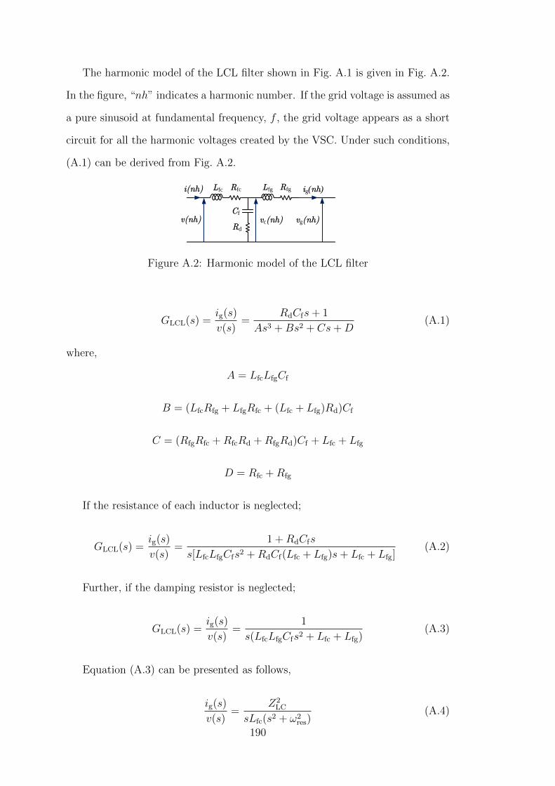
The harmonic model of the LCL filter shown in Fig. A.1 is given in Fig. A.2.
In the figure, “nh” indicates a harmonic number. If the grid voltage is assumed as
a pure sinusoid at fundamental frequency, f , the grid voltage appears as a short
circuit for all the harmonic voltages created by the VSC. Under such conditions,
(A.1) can be derived from Fig. A.2.
Lfc Lfg
Rd
Cf
Rfc Rfg ig(nh)
vg(nh)vc(nh)v(nh)
i(nh)
Figure A.2: Harmonic model of the LCL filter
GLCL(s) =ig(s)
v(s)=
RdCfs+ 1
As3 +Bs2 + Cs+D(A.1)
where,
A = LfcLfgCf
B = (LfcRfg + LfgRfc + (Lfc + Lfg)Rd)Cf
C = (RfgRfc +RfcRd +RfgRd)Cf + Lfc + Lfg
D = Rfc +Rfg
If the resistance of each inductor is neglected;
GLCL(s) =ig(s)
v(s)=
1 +RdCfs
s[LfcLfgCfs2 +RdCf(Lfc + Lfg)s+ Lfc + Lfg](A.2)
Further, if the damping resistor is neglected;
GLCL(s) =ig(s)
v(s)=
1
s(LfcLfgCfs2 + Lfc + Lfg)(A.3)
Equation (A.3) can be presented as follows,
ig(s)
v(s)=
Z2LC
sLfc(s2 + ω2res)
(A.4)
190

where Z2LC = 1/LfgCf and ω2
res = (Lfc + Lfg)/LfcLfgCf .
Switching frequency (fsw) current harmonics are dominant in the output cur-
rent of the VSC. Therefore, the LCL filter design procedure will follow to reduce
the switching ripple current that flows to the grid. The switching ripple current
attenuation by the LCL filter at any frequency can be derived in two ways. First,
it is derived assuming that the filter capacitance has very small impedance at high
frequencies. Therefore the capacitor branch can be considered as short circuited.
Hence, with that assumption, the following relationship between the converter
side current and voltage can be derived.
i(s)
v(s)≈ 1
sLfc
(A.5)
From (A.4) and (A.5);
ig(s)
i(s)≈ Z2
LC
(s2 + ω2res)
(A.6)
As the second method, the transfer function for the switching ripple current
attenuation can be derived as given in (A.7) without the assumption used to
derive (A.6) and considering that the grid voltage appears as short circuited for
harmonics.
ig(s)
i(s)=
Z2LC
(s2 + Z2LC)
(A.7)
The assumption made to derive (A.6) is for the purpose of developing a re-
lationship between Lfc, Lfg and Cf for frequencies higher than the switching fre-
quency of the VSC, fsw. The assumption will be justified while analysing the
performance of a designed LCL filter.
Defining base quantities for the VSC system;
Zb =V 2
r
Pr
(A.8)
191

Cb =1
ωZb
(A.9)
A.2 Design constraints of LCL filter component sizes
1. The capacitance of Cf is limited by the amount of reactive power absorbed
by the capacitor (generally less than 0.05Pr).
2. To limit the AC voltage drop during operation, the total value of inductive
reactance, (ωLfc+ωLfg) should be less than 0.1 pu at fundamental frequency.
3. The resonant frequency should be in the range 10f < fres <12fsw to avoid
resonance problems. fres is the resonant frequency of the LCL filter.
4. The damping resistor, Rd should be large enough to provide sufficient damp-
ing at the resonant frequency of the LCL filter but losses cannot be very
high.
A.3 Design procedure of an LCL filter
1. Determine the switching current ripple through the converter side inductor
and establish the inductance of Lfc. Then the grid side inductor of the LCL
filter, Lfg can be expressed as a function of Lfc, using an index, r.
Lfg = rLfc (A.10)
2. If x is the percentage of reactive power absorbed under rated condition as
mentioned in Constraint 1, the maximum capacitance of Cf can be calcu-
lated as follows.
Cf = xCb (A.11)
3. Equation (A.6) can be rearranged as (A.12) where a = LCbω2sw. A value
for r can be calculated using (A.12) for a given switching ripple current
192
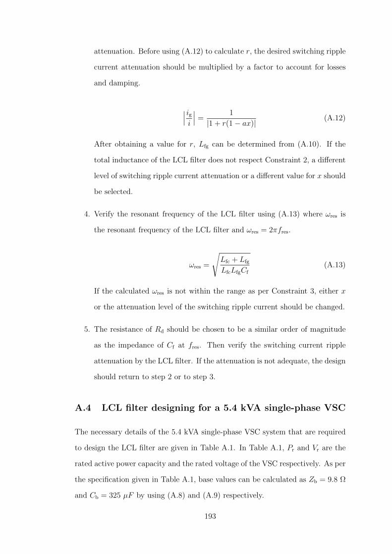
attenuation. Before using (A.12) to calculate r, the desired switching ripple
current attenuation should be multiplied by a factor to account for losses
and damping.
∣∣∣igi
∣∣∣ =1
|1 + r(1− ax)| (A.12)
After obtaining a value for r, Lfg can be determined from (A.10). If the
total inductance of the LCL filter does not respect Constraint 2, a different
level of switching ripple current attenuation or a different value for x should
be selected.
4. Verify the resonant frequency of the LCL filter using (A.13) where ωres is
the resonant frequency of the LCL filter and ωres = 2πfres.
ωres =
√Lfc + Lfg
LfcLfgCf
(A.13)
If the calculated ωres is not within the range as per Constraint 3, either x
or the attenuation level of the switching ripple current should be changed.
5. The resistance of Rd should be chosen to be a similar order of magnitude
as the impedance of Cf at fres. Then verify the switching current ripple
attenuation by the LCL filter. If the attenuation is not adequate, the design
should return to step 2 or to step 3.
A.4 LCL filter designing for a 5.4 kVA single-phase VSC
The necessary details of the 5.4 kVA single-phase VSC system that are required
to design the LCL filter are given in Table A.1. In Table A.1, Pr and Vr are the
rated active power capacity and the rated voltage of the VSC respectively. As per
the specification given in Table A.1, base values can be calculated as Zb = 9.8 Ω
and Cb = 325 µF by using (A.8) and (A.9) respectively.
193
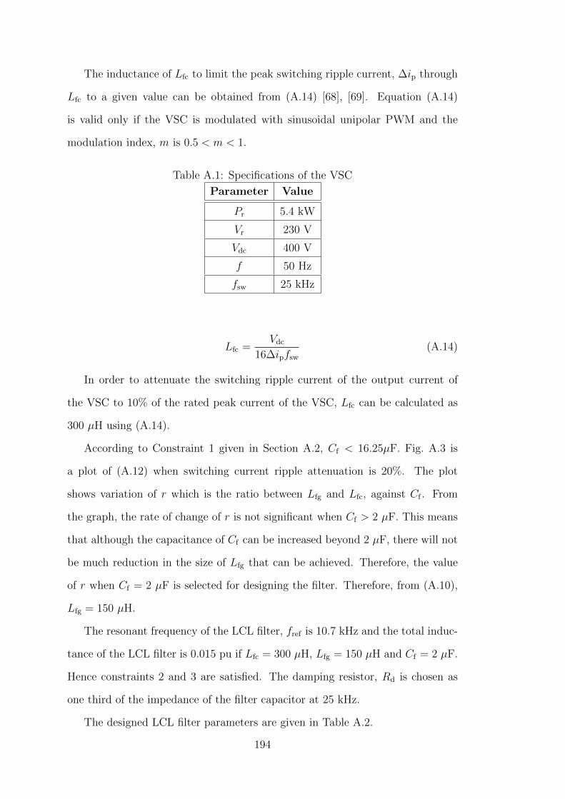
The inductance of Lfc to limit the peak switching ripple current, ∆ip through
Lfc to a given value can be obtained from (A.14) [68], [69]. Equation (A.14)
is valid only if the VSC is modulated with sinusoidal unipolar PWM and the
modulation index, m is 0.5 < m < 1.
Table A.1: Specifications of the VSC
Parameter Value
Pr 5.4 kW
Vr 230 V
Vdc 400 V
f 50 Hz
fsw 25 kHz
Lfc =Vdc
16∆ipfsw
(A.14)
In order to attenuate the switching ripple current of the output current of
the VSC to 10% of the rated peak current of the VSC, Lfc can be calculated as
300 µH using (A.14).
According to Constraint 1 given in Section A.2, Cf < 16.25µF. Fig. A.3 is
a plot of (A.12) when switching current ripple attenuation is 20%. The plot
shows variation of r which is the ratio between Lfg and Lfc, against Cf . From
the graph, the rate of change of r is not significant when Cf > 2 µF. This means
that although the capacitance of Cf can be increased beyond 2 µF, there will not
be much reduction in the size of Lfg that can be achieved. Therefore, the value
of r when Cf = 2 µF is selected for designing the filter. Therefore, from (A.10),
Lfg = 150 µH.
The resonant frequency of the LCL filter, fref is 10.7 kHz and the total induc-
tance of the LCL filter is 0.015 pu if Lfc = 300 µH, Lfg = 150 µH and Cf = 2 µF.
Hence constraints 2 and 3 are satisfied. The damping resistor, Rd is chosen as
one third of the impedance of the filter capacitor at 25 kHz.
The designed LCL filter parameters are given in Table A.2.
194
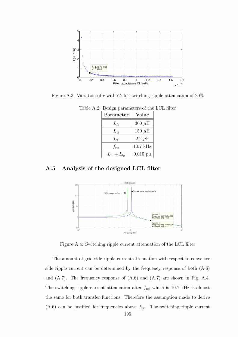
0 0.2 0.4 0.6 0.8 1 1.2 1.4 1.6 1.8
x 10−5
0
1
2
3
4
5
X: 1.787e−006Y: 0.4905
Filter capacitance Cf / (uF)
Lg/L
or
(r)
Figure A.3: Variation of r with Cf for switching ripple attenuation of 20%
Table A.2: Design parameters of the LCL filter
Parameter Value
Lfc 300 µH
Lfg 150 µH
Cf 2.2 µF
fres 10.7 kHz
Lfc + Lfg 0.015 pu
A.5 Analysis of the designed LCL filter
Bode Diagram
Frequency (Hz)
103
104
105
−50
0
50
100
150
System: HFrequency (Hz): 2.49e+004Magnitude (dB): −17
System: GFrequency (Hz): 2.49e+004Magnitude (dB): −16.3
Mag
nitu
de (
dB)
Without assumptionWith assumption
Figure A.4: Switching ripple current attenuation of the LCL filter
The amount of grid side ripple current attenuation with respect to converter
side ripple current can be determined by the frequency response of both (A.6)
and (A.7). The frequency response of (A.6) and (A.7) are shown in Fig. A.4.
The switching ripple current attenuation after fres which is 10.7 kHz is almost
the same for both transfer functions. Therefore the assumption made to derive
(A.6) can be justified for frequencies above fsw. The switching ripple current
195

attenuation at fsw, which is determined from two plots in Fig. A.4, is less than
20%. Hence the designed LCL filter parameters given in Table A.2 satisfy the
design requirements.
196
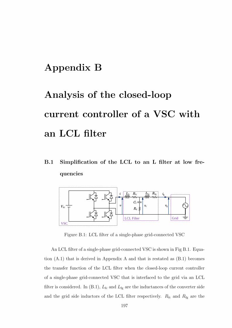
Appendix B
Analysis of the closed-loop
current controller of a VSC with
an LCL filter
B.1 Simplification of the LCL to an L filter at low fre-
quencies
Grid
Lfc Lfg
Rd
Cf
Rfc Rfg ig
vg
LCL Filter
Vdc
VSC
vcv
i
Figure B.1: LCL filter of a single-phase grid-connected VSC
An LCL filter of a single-phase grid-connected VSC is shown in Fig B.1. Equa-
tion (A.1) that is derived in Appendix A and that is restated as (B.1) becomes
the transfer function of the LCL filter when the closed-loop current controller
of a single-phase grid-connected VSC that is interfaced to the grid via an LCL
filter is considered. In (B.1), Lfc and Lfg are the inductances of the converter side
and the grid side inductors of the LCL filter respectively. Rfc and Rfg are the
197

resistances of inductors of the LCL filter. The damping resistor is Rd and that is
connected in series with the filter capacitor, Cf . v is the voltage at the output of
the VSC and ig is the current injected to the grid by the VSC.
GLCL(s) =ig(s)
v(s)=
RdCfs+ 1
As3 +Bs2 + Cs+D(B.1)
where,
A = LfcLfgCf
B = (LfcRfg + LfgRfc + (Lfc + Lfg)Rd)Cf
C = (RfcRfg +RfcRd +RfgRd)Cf + Lfc + Lfg
D = Rfc +Rfg.
The transfer function an L only filter can be obtained from (B.1) if Cf = 0
and that is given in (B.2).
GL(s) =ig(s)
v(s)=
1
(Lfc + Lfg)s+Rfc +Rfg
(B.2)
The frequency responses of (B.1) and (B.2) are shown in Fig. B.2 when Rfc,
Rfg, andRd are assumed to have negligible resistances. The frequency responses of
both the LCL filter and the L filter below the resonant frequency of the LCL filter
is almost similar as that can be seen in the Fig B.2. Both types of filters attenuate
signals of frequencies less than the resonant frequency by −20 dB/decade. If the
desired bandwidth of the closed-loop current controller of the VSC is 500 Hz that
is far less than the resonant frequency of the LCL filter. Hence, the LCL filter
can be simplified to an L filter while designing the closed-loop current controller.
198

−150
−100
−50
0
50
100
150
Mag
nitu
de (
dB)
100
101
102
103
104
105
−270
−225
−180
−135
−90P
hase
(de
g)
Bode Diagram
Frequency (Hz)
LCL Filter
L Filter
Figure B.2: Frequency responses of an LCL and an L filter
B.2 Effect of the damping resistor in the LCL filter on the
dynamic stability of the closed-loop current controller
of the VSC
A simplified block diagram of the closed-loop current controller of the VSC is
shown in Fig. B.3. In Fig. B.3, GLCL(s) is the transfer function of the LCL filter
that is given in (B.1) and C(s) is a proportional resonant (PR) regulator. The
transfer function of the PR regulator that includes both fundamental frequency
compensator and low-order odd harmonic compensators (HC), is given in (B.3)
where kpc is the proportional gain, kich is the integral gain and ωc is the 3 dB
cut-off frequency and ω0 = 100π rad/s.
C(s)ig
igrefig
GLCL(s)
Figure B.3: Simplified block diagram of the closed-loop current controller
C(s) = kpc +∑
h=1,3,5,7
2kichωcs
s2 + 2ωcs+ (hω0)2(B.3)
199

The open-loop and closed-loop transfer functions of the current controller
shown in Fig B.3 are given in (B.4) and (B.5) respectively.
Gol(s) = C(s)GLCL(s) (B.4)
Gcl(s) =C(s)GLCL(s)
1 + C(s)GLCL(s)(B.5)
In the LCL filter shown in Fig B.1, Lfc = 300 µH, Lfg = 150 µH, Cf = 2.2 µF
and Rfc, Rfg = 0.001 Ω. In the PR regulator that is given in (B.3), kpc = 4 ,
kic1 = 100, kich = 80 (h = 3, 5, 7) and the 3 dB cut-off frequency, ωc, is 5 rad/s.
The pole and zero plot of (B.4) is shown in Fig. B.4 when Rd = 0. Rfc and
Rfc, which are the resistances of inductors in the LCL filter, are assumed to have
negligible values when plotting Fig. B.4.
Pole−Zero Map
Real Axis
Imag
inar
y A
xis
−140 −120 −100 −80 −60 −40 −20 0−8
−6
−4
−2
0
2
4
6
8x 10
4
System: OLPole : 0 + 6.74e+004iDamping: −0Overshoot (%): 100Frequency (Hz): 1.07e+004
Figure B.4: Pole and zero plot of open-loop system without damping
In Fig. B.4, there are two poles on the imaginary axis that are further away
from the origin. Hence the closed-loop current controller is unstable when Rd =
0 Ω. These unstable poles are the resonant poles of the LCL filter.
The stability of the closed-loop current controller can be improved by adding a
damping resistor, Rd in series with the LCL filter capacitor Cf [60]. The addition
of the damping resistor, Rd creates an additional zero while attracting unstable
poles towards negative side of the imaginary axis in the complex plane and hence
200

improve the stability of the closed-loop current controller.
The positions of poles and zeros of the open-loop system after adding the
damping resistor, Rd, in series with the filter capacitor, Cf , is shown in Fig. B.5
for a range of values of Rd. As shown in Fig. B.5, the unstable poles of the open-
loop system have moved to the left hand side of the imaginary axis in the complex
plan. Hence the stability of the closed-loop current controller is improved with
addition of Rd.
Pole−Zero Map
Real Axis
Imag
inar
y A
xis
−2.5 −2 −1.5 −1 −0.5 0 0.5
x 105
−8
−6
−4
−2
0
2
4
6
8x 10
4
Rd = 0 ohm
Rd = 2 ohm
Rd = 4 ohm
Rd = 6 ohm
Figure B.5: Pole and zero plot of open-loop system with damping
The Bode plots of (B.4) with and without Rd are shown in Fig. B.6 in which
resonant peaks at low frequencies are due to the PR regulator and the resonant
peak at around 10.7 kHz is because of the LCL filter. The resonant peak caused
by the LCL filter has been reduced once Rd is added. The stability of the closed-
loop current controller improves with increasing damping resistor values, while
the attenuation provided the LCL filter for high frequency signals has reduced.
Since a higher damping resistor increases resistive losses in the system, a small
resistor should be selected which can improve system stability while minimising
the losses. In this work, the damping resistor, Rd is chosen as one third of the
impedance of the filter capacitor at the resonant frequency frequency of the LCL
filter, fres [60]. The impedance of filter capacitor at fres is 7 Ω. Hence Rd is
chosen as 2 Ω.
201

−200
−100
0
100
200
300
400
Mag
nitu
de (
dB)
100
101
102
103
104
105
106
−450
−360
−270
−180
−90
0
Pha
se (
deg)
Bode Diagram
Frequency (Hz)
Rd = 0 ohm
Rd = 2 ohm
Rd = 4 ohm
Rd = 6 ohmResonance of PR controller
Resonance of LCL filter
Figure B.6: Frequency response of the open-loop system
B.3 Effect of the grid impedance on the performance of
the LCL filter and the closed-loop current controller
of the VSC
The LCL filter was designed using the procedure stated in Appendix A considering
that the grid impedance is zero. In a real world application, the LCL filter is the
front end of a VSC that is connected to the grid. Hence studying the effects of
the grid impedance on the performance of the LCL filter is important. Further,
the performance of the closed-loop current controller should be evaluated in the
presence of the grid impedance as well.
In the following analysis, the grid impedance (0.4 + j0.25 Ω) is lumped with
the grid side inductance, Lfg and the resistance, Rfg of the LCL filter. Further,
resistances of filter components are neglected.
The Bode plot of the open-loop current controller is shown in Fig. B.7 for two
different cases. As shown in Fig. B.7 the resonant frequency of the LCL filter
without the grid impedance is 10.7 kHz. Once the grid impedance is added to the
system, the resonant frequency of the LCL filter has dropped to 7.1 kHz which is
about a 33% reduction from the previous value. The performance of the LCL filter
with respect to attenuating high frequency harmonics has improved with addition
202
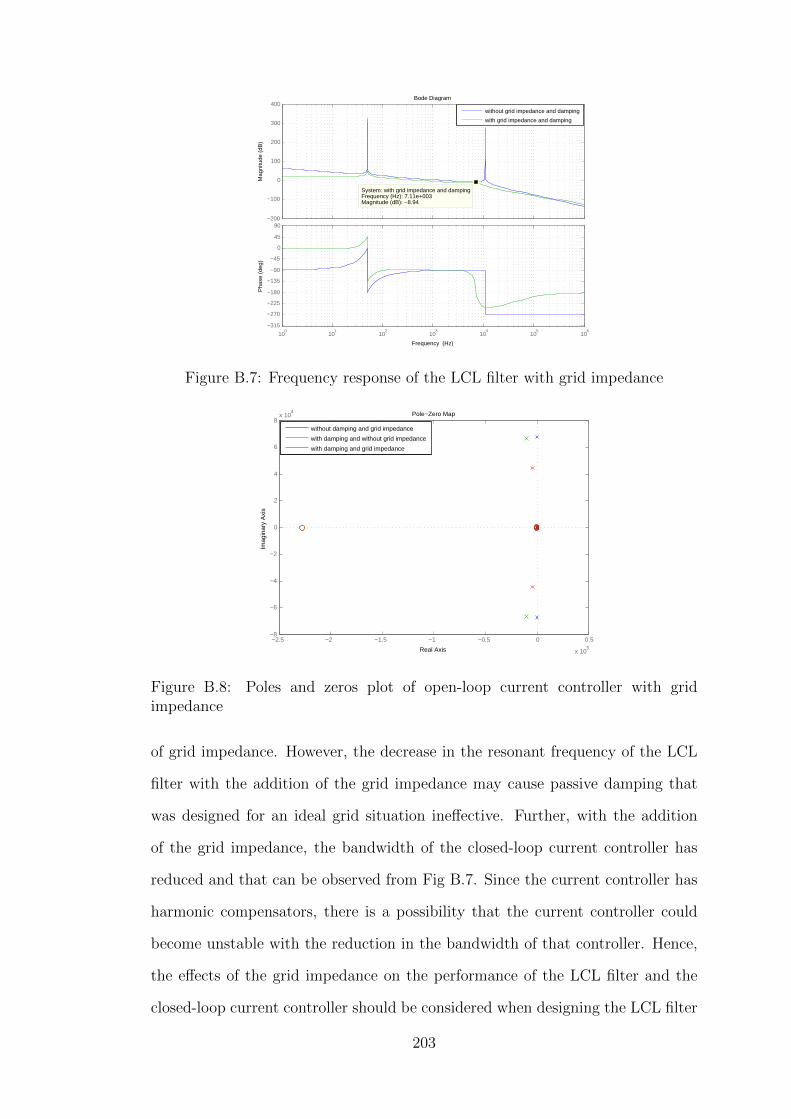
100
101
102
103
104
105
106
−315
−270
−225
−180
−135
−90
−45
0
45
90
Pha
se (
deg)
Bode Diagram
Frequency (Hz)
−200
−100
0
100
200
300
400
System: with grid impedance and dampingFrequency (Hz): 7.11e+003Magnitude (dB): −8.94
Mag
nitu
de (
dB)
without grid impedance and damping
with grid impedance and damping
Figure B.7: Frequency response of the LCL filter with grid impedance
−2.5 −2 −1.5 −1 −0.5 0 0.5
x 105
−8
−6
−4
−2
0
2
4
6
8x 10
4
Pole−Zero Map
Real Axis
Imag
inar
y A
xis
without damping and grid impedance
with damping and without grid impedance
with damping and grid impedance
Figure B.8: Poles and zeros plot of open-loop current controller with gridimpedance
of grid impedance. However, the decrease in the resonant frequency of the LCL
filter with the addition of the grid impedance may cause passive damping that
was designed for an ideal grid situation ineffective. Further, with the addition
of the grid impedance, the bandwidth of the closed-loop current controller has
reduced and that can be observed from Fig B.7. Since the current controller has
harmonic compensators, there is a possibility that the current controller could
become unstable with the reduction in the bandwidth of that controller. Hence,
the effects of the grid impedance on the performance of the LCL filter and the
closed-loop current controller should be considered when designing the LCL filter
203
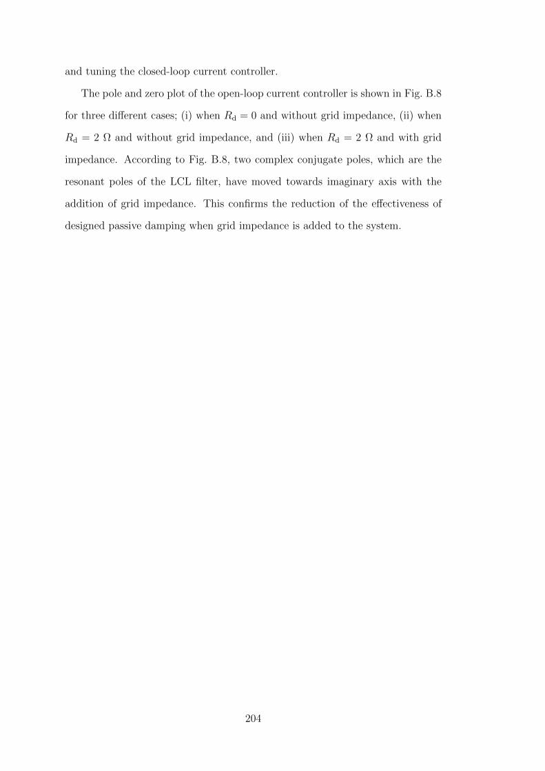
and tuning the closed-loop current controller.
The pole and zero plot of the open-loop current controller is shown in Fig. B.8
for three different cases; (i) when Rd = 0 and without grid impedance, (ii) when
Rd = 2 Ω and without grid impedance, and (iii) when Rd = 2 Ω and with grid
impedance. According to Fig. B.8, two complex conjugate poles, which are the
resonant poles of the LCL filter, have moved towards imaginary axis with the
addition of grid impedance. This confirms the reduction of the effectiveness of
designed passive damping when grid impedance is added to the system.
204
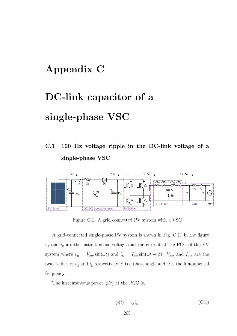
Appendix C
DC-link capacitor of a
single-phase VSC
C.1 100 Hz voltage ripple in the DC-link voltage of a
single-phase VSC
Grid
2Lfc 2Lfg
Rd
Cf
2Rfc 2Rfg
CdcCpvLg Rg
Ldc DdcigIpv
Vpvvg
LCL Filter
Vdc
H-BridgeDC-DC Boost ConverterPV Array
Ppv Pdc Pc , Qc Pg , Qg
vs
Figure C.1: A grid connected PV system with a VSC
A grid-connected single-phase PV system is shown in Fig. C.1. In the figure
vg and ig are the instantaneous voltage and the current at the PCC of the PV
system where vg = Vgm sin(ωt) and ig = Igm sin(ωt − φ). Vgm and Igm are the
peak values of vg and ig respectively, φ is a phase angle and ω is the fundamental
frequency.
The instantaneous power, p(t) at the PCC is,
p(t) = vgig (C.1)
205
p(t) = VgmIgm sin(ωt) sin(ωt− φ). (C.2)
Equation (C.2) can be simplified given in (C.3).
p(t) =1
2VgmIgm cosφ[1− cos(2ωt)]− 1
2VgmIgm sinφ sin(2ωt) (C.3)
If P = 12VgmIgm cosφ and Q = 1
2VgmIgm sinφ where P is the average active
power and Q is the average reactive power, assigning these values in (C.3), (C.4)
can be derived.
p(t) = P [1− cos(2ωt)]−Q sin(2ωt) (C.4)
The instantaneous power variation on the AC side of the VSC that is given
in (C.4) is plotted in Fig. C.2 when P = 1 and Q = 1. According to (C.4) and
Fig. C.2, in a single-phase system, the active power delivered to the grid has an
average value of P (which is 1 in this particular case) and an oscillating component
that is −P cos(2ωt). The active power flow is unidirectional since the active
power component in (C.4) never becomes negative when power is injecting to the
grid. Unlike the active power component, the reactive power component only
has an oscillating component, that oscillates at twice the fundamental frequency.
Therefore the average value of the reactive power delivered to the grid over half
a cycle is zero.
The PV array generates only DC power. Hence, Ppv in Fig. C.1 is DC power
which is equal to the average power P if the losses in the converter system are
disregarded. However, the grid side of the single-phase VSC demands not only
the constant active power that can be supplied by the PV but also an oscillating
component of active power. The oscillating active power component cannot be
supplied by the PV array. Therefore, there is a mismatch in the instantaneous
power demand from the AC side and the available power from the PV array. In
single-phase VSCs, the DC-link capacitor, (Cdc) is used to balance the power mis-
206

0 0.005 0.01 0.015 0.02 0.025 0.03 0.035 0.04−1
−0.5
0
0.5
1
1.5
2
Time (s)
Active(P
)an
dReactive(Q
)Power
(pu) P
Q
Figure C.2: Variation of the active and the reactive power delivered to the gridin a single-phase VSC
match. When the AC side power demand is less than that is generated by the PV
array, the DC-link capacitor, Cdc, charges by storing excess energy, whereas when
the demand is higher than generated power from the PV array, Cpv discharges
by releasing stored energy. The charging and discharging of Cdc causes a voltage
ripple at the DC-link. The frequency of the ripple is equal to the frequency of
active power oscillation that is twice the fundamental frequency.
In half a cycle that is 10 ms, the energy transfered to the grid as reactive power
is zero. Therefore the amount of energy drawn from the PV array to generate
reactive power is zero. Within a quarter cycle, for example, from t = 0.005 ms
to t = 0.010 ms in Fig. C.2, capacitor Cdc releases a certain amount of energy
as the reactive power to the grid and within the next quarter cycle the capacitor
stores the same amount of energy. The energy transfer as the reactive power
also causes voltage oscillations at the DC-link at a similar frequency as the active
power transfer does.
C.2 Selection of the DC-link capacitor value
An expression for the energy oscillation at the AC side of the VSC can be obtained
by considering only the oscillating power components of (C.4) and integrating
207
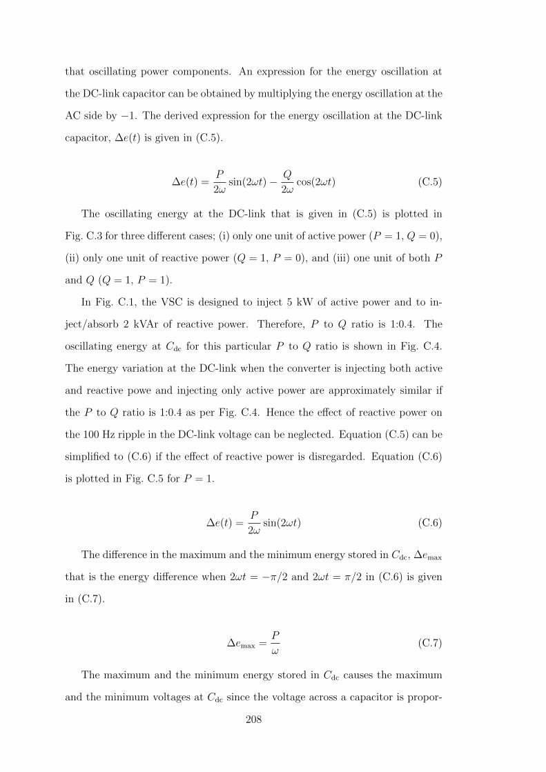
that oscillating power components. An expression for the energy oscillation at
the DC-link capacitor can be obtained by multiplying the energy oscillation at the
AC side by −1. The derived expression for the energy oscillation at the DC-link
capacitor, ∆e(t) is given in (C.5).
∆e(t) =P
2ωsin(2ωt)− Q
2ωcos(2ωt) (C.5)
The oscillating energy at the DC-link that is given in (C.5) is plotted in
Fig. C.3 for three different cases; (i) only one unit of active power (P = 1, Q = 0),
(ii) only one unit of reactive power (Q = 1, P = 0), and (iii) one unit of both P
and Q (Q = 1, P = 1).
In Fig. C.1, the VSC is designed to inject 5 kW of active power and to in-
ject/absorb 2 kVAr of reactive power. Therefore, P to Q ratio is 1:0.4. The
oscillating energy at Cdc for this particular P to Q ratio is shown in Fig. C.4.
The energy variation at the DC-link when the converter is injecting both active
and reactive powe and injecting only active power are approximately similar if
the P to Q ratio is 1:0.4 as per Fig. C.4. Hence the effect of reactive power on
the 100 Hz ripple in the DC-link voltage can be neglected. Equation (C.5) can be
simplified to (C.6) if the effect of reactive power is disregarded. Equation (C.6)
is plotted in Fig. C.5 for P = 1.
∆e(t) =P
2ωsin(2ωt) (C.6)
The difference in the maximum and the minimum energy stored in Cdc, ∆emax
that is the energy difference when 2ωt = −π/2 and 2ωt = π/2 in (C.6) is given
in (C.7).
∆emax =P
ω(C.7)
The maximum and the minimum energy stored in Cdc causes the maximum
and the minimum voltages at Cdc since the voltage across a capacitor is propor-
208
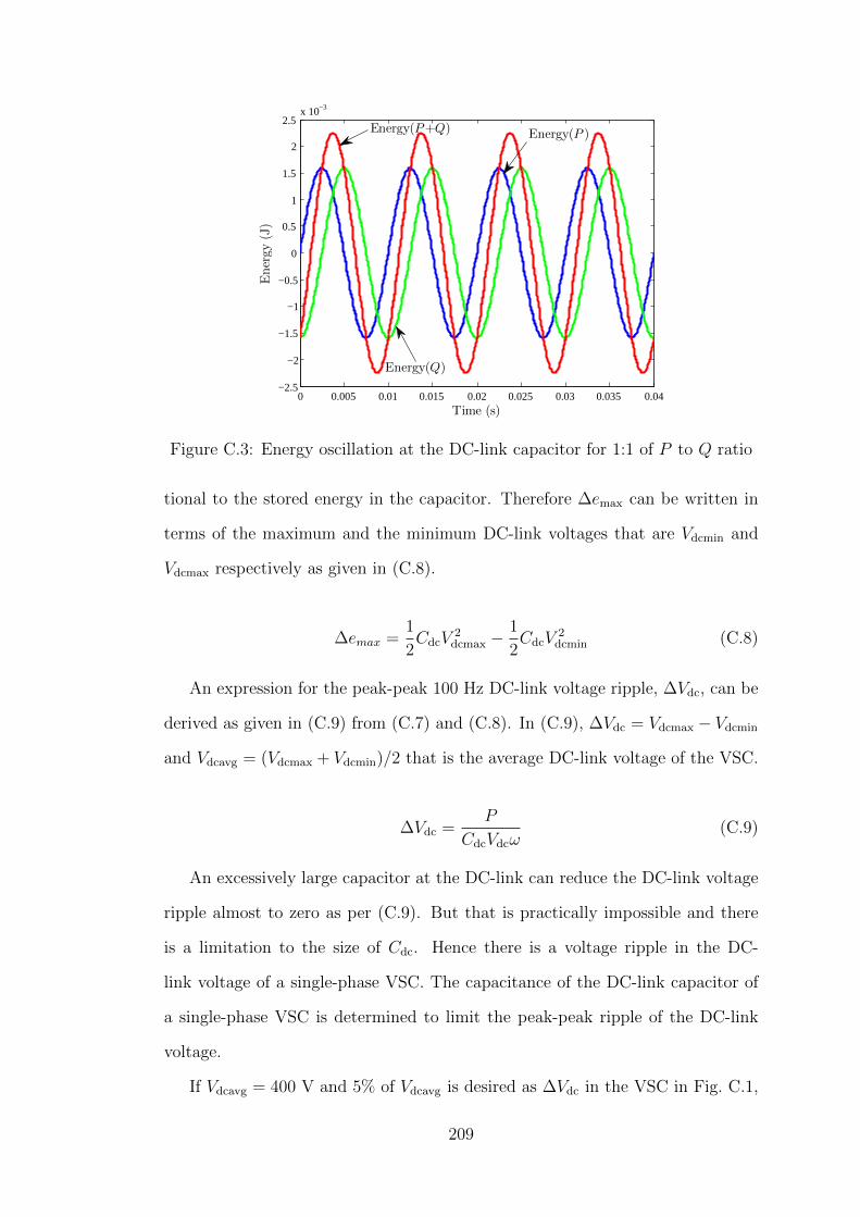
0 0.005 0.01 0.015 0.02 0.025 0.03 0.035 0.04−2.5
−2
−1.5
−1
−0.5
0
0.5
1
1.5
2
2.5x 10⁻³
Time (s)
Energy(J)
Energy(P+Q)
Energy(Q)
Energy(P )
Figure C.3: Energy oscillation at the DC-link capacitor for 1:1 of P to Q ratio
tional to the stored energy in the capacitor. Therefore ∆emax can be written in
terms of the maximum and the minimum DC-link voltages that are Vdcmin and
Vdcmax respectively as given in (C.8).
∆emax =1
2CdcV
2dcmax −
1
2CdcV
2dcmin (C.8)
An expression for the peak-peak 100 Hz DC-link voltage ripple, ∆Vdc, can be
derived as given in (C.9) from (C.7) and (C.8). In (C.9), ∆Vdc = Vdcmax − Vdcmin
and Vdcavg = (Vdcmax + Vdcmin)/2 that is the average DC-link voltage of the VSC.
∆Vdc =P
CdcVdcω(C.9)
An excessively large capacitor at the DC-link can reduce the DC-link voltage
ripple almost to zero as per (C.9). But that is practically impossible and there
is a limitation to the size of Cdc. Hence there is a voltage ripple in the DC-
link voltage of a single-phase VSC. The capacitance of the DC-link capacitor of
a single-phase VSC is determined to limit the peak-peak ripple of the DC-link
voltage.
If Vdcavg = 400 V and 5% of Vdcavg is desired as ∆Vdc in the VSC in Fig. C.1,
209
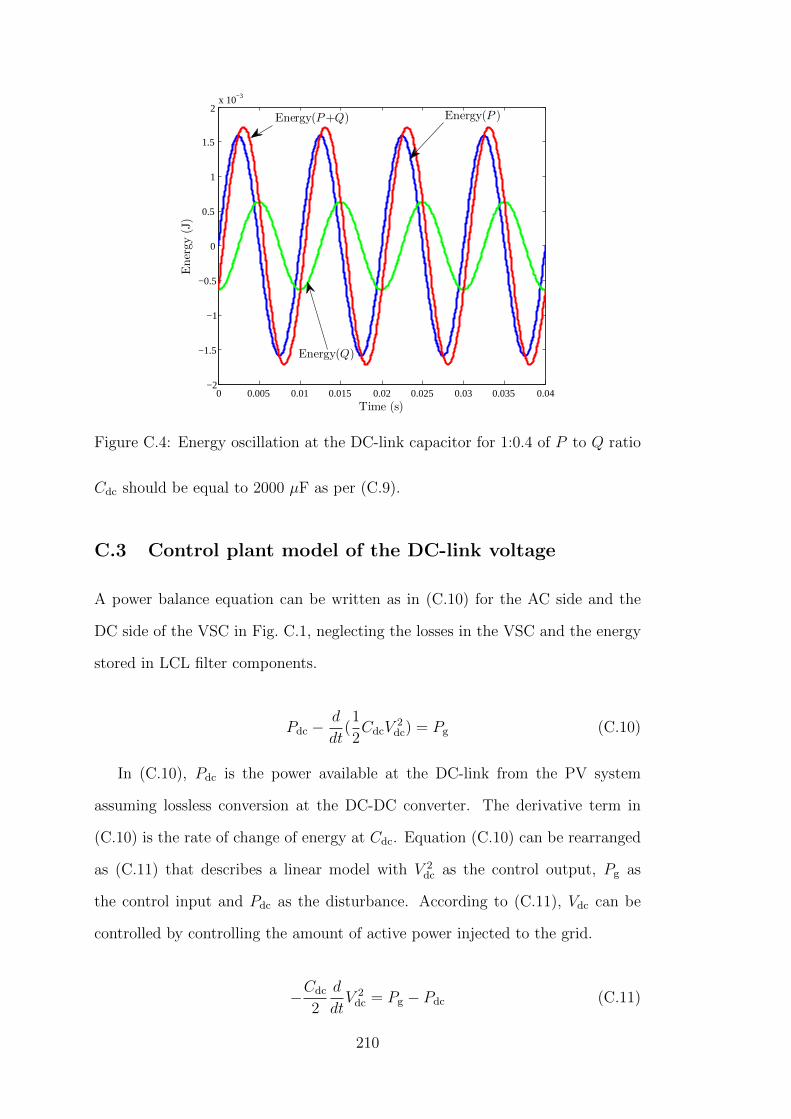
0 0.005 0.01 0.015 0.02 0.025 0.03 0.035 0.04−2
−1.5
−1
−0.5
0
0.5
1
1.5
2x 10⁻³
Time (s)
Energy
(J)
Energy(P )
Energy(Q)
Energy(P+Q)
Figure C.4: Energy oscillation at the DC-link capacitor for 1:0.4 of P to Q ratio
Cdc should be equal to 2000 µF as per (C.9).
C.3 Control plant model of the DC-link voltage
A power balance equation can be written as in (C.10) for the AC side and the
DC side of the VSC in Fig. C.1, neglecting the losses in the VSC and the energy
stored in LCL filter components.
Pdc −d
dt(1
2CdcV
2dc) = Pg (C.10)
In (C.10), Pdc is the power available at the DC-link from the PV system
assuming lossless conversion at the DC-DC converter. The derivative term in
(C.10) is the rate of change of energy at Cdc. Equation (C.10) can be rearranged
as (C.11) that describes a linear model with V 2dc as the control output, Pg as
the control input and Pdc as the disturbance. According to (C.11), Vdc can be
controlled by controlling the amount of active power injected to the grid.
−Cdc
2
d
dtV 2
dc = Pg − Pdc (C.11)
210

0 0.005 0.01 0.015 0.02 0.025 0.03 0.035 0.04−2
−1.5
−1
−0.5
0
0.5
1
1.5
2x 10⁻³
Time (s)
Energy
(J)
Energy(P)
Figure C.5: Energy oscillation at the DC-link capacitor for one unit of activepower
The transfer function of the control plant model for the DC-link voltage is
given in (C.12).
GVdc(s) =V 2
dc(s)
Pg(s)= − 2
Cdcs(C.12)
211

212

Appendix D
Experimental Setup
D.1 Introduction
In order to validate the simulation model of a grid-connected single-phase, two-
stage photovoltaic system that was developed in PSCAD/EMTDC simulation
program, an experimental setup was needed. Therefore a laboratory scale experi-
mental setup of two, 5 kW grid-connected single-phase, two-stage PV systems was
implemented after acquiring necessary hardware and using the control algorithms
developed in the simulation model. The implemented experimental setup is used
for validating the simulation model and also for identifying operational and con-
trol interactions between multiple PV systems when PV systems are operated
electrically very close to each other.
D.2 System description of the experimental setup
A schematic diagram of the implemented experimental setup of the grid connected
PV system is shown in Fig. D.1. A picture of the complete experimental setup
implemented is shown in Fig. D.1
213

Grid
LfcL
fg
Rd
Cf
RfcR
fg
CdcC
pv
LfcR
fcL
fgR
fg
LglR
gl
LgnR
gn
LdcD
dcFu
seR
elay
con
tact
s
i g
I pv
Vpvv g
LCL
Filte
r
Vdc
H-B
ridge
DC
-DC
Boo
st C
onve
rter
PV S
imul
ator
SEM
IKR
ON
Mod
ule
dSPA
CE
– D
S110
4 co
ntro
ller
Dig
ital I
/O In
terf
ace
and
rela
y dr
iver
circ
uit
Inte
rfac
e bo
ard
for s
igna
l con
ditio
ning
Gat
e dr
ive
puls
esEr
ror s
igna
l
Bre
aker
Erro
r Sig
nal
Cur
rent
feed
back
Vol
tage
sens
ors
Vol
tage
fe
edba
ckS dc
Fig
ure
D.1
:Sch
emat
icdia
gram
ofth
eex
per
imen
tal
setu
p
214

Fig
ure
D.2
:P
ictu
reof
the
com
ple
teex
per
imen
tal
setu
p
215
The implemented PV system consists of a two-stage converter that was formed
by a combination of a DC-DC boost converter and a VSC. The PV system is
interfaced to the grid via an LCL filter. A brief description of various modules
and some of the important components shown in Fig. D.1 are given in following
subsections.
D.2.1 SEMITEACH-IGBT stack
Figure D.3: The Semikron SEMITEACH-IGBT stack
The Semikron SEMITEACH-IGBT stack that was used in the experimental
setup is shown in Fig. D.3. This module was used to form most of the power
electronic circuitry of the two-stage converter. In the experimental setup, two
legs of the 3-phase inverter built into the Semikron SEMITEACH-IGBT stack
was used to form the full-bridge. Further, the diode (Ddc) and the power elec-
tronic switch, Sdc that are parts of the DC-DC boost converter and the DC-link
capacitor, Cdc are integrated components of the Semikron SEMITEACH-IGBT
stack. The full-bridge in combination with Cdc forms the VSC that is the DC-AC
power converter of the PV system. All power electronic switches in the module
are IGBTs.
The Semikron SEMITEACH-IGBT stack has built-in IGBT drivers for each
leg of the 3-phase inverter built into the stack. The driver imposes roughly a 4 µs
216
dead-time on top and bottom switches of a leg in order to avoid a short-circuit
condition in the power circuit. The IGBT drivers should be supplied with an
external 15 V DC power supply. The IGBT driver generates an error in cases
where the driver detects a power supply undervoltage condition or an over current
condition through an IGBT of the stack. If the driver detects an error, the IGBT
is turned off. The error signal that is generated by the driver of each leg is
accessible from outside of the stack. Hence in the experimental setup these error
signals are integrated to the control circuit to develop protective measures.
D.2.2 LCL filter
The LCL filter minimises the amount of switching frequency harmonic current
injected to the grid by the PV system. There were two types of LCL filter
configurations considered while implementing the experimental setup and those
two configurations are shown in Fig. D.4 where Lfc is the converter side inductance
and Lfg is the grid side inductance. Rfc and Rfg are resistances of converter side
and grid side inductors respectively. Cf is the filter capacitor and Rd is the
damping resistor.
In the experimental setup, the switching frequency of both the DC-DC boost
converter and the VSC are 10 kHz and bipolar sinusoidal pulse width modulation
(bipolar-SPWM) was used to switch the IGBTs in the VSC due to limitations
in the dSPACE-DS1104 controller. Since the LCL filter configuration shown in
Fig. D.4(b) leads to less ground leakage current when the VSC is switched with
bipolar-SPWM technique, that particular LCL filter configuration is used in the
implemented experimental setup of the PV system.
The LCL filter was initially designed by following the procedures described in
Appendix A. However, when purchasing inductors for the LCL filter rather than
adopting component values that are optimally designed (in terms of inductances
and capacitance) a conservative design approach was followed. A considerable
margin was allowed for design errors when deciding the component values to pur-
217

Lfc Lfg
Rd
Cf
Rfc Rfg
Lfc Rfc Lfg Rfg
2Lfc 2Lfg
Rd
Cf
2Rfc 2Rfg
(a) (b)
Figure D.4: LCL filter configurations
chase but the design rules depicted in Appendix A were not violated. The values
of the components of the LCL filter as used in the implemented experimental
setup of the PV system are Lfc = 900 µH, Lfg = 450 µH, Cf = 4.7 µF and
Rd = 2 Ω.
D.2.3 PV emulator
The PV emulator simulates the electrical characteristics (I-V curve) of a defined
PV array. An ELGAR TerraSAS ETS1000X PV emulator is used in the experi-
mental setup. The front view of the ELGAR TerraSAS ETS1000X PV emulator
is shown in Fig D.5.
Figure D.5: The front view of a ELGAR TerraSAS ETS1000X PV emulator
The maximum output power, output current and output voltage of the EL-
GAR TerraSAS ETS1000X PV emulator are 8.5 kW (at 0.85 fill factor), 10 A DC
and 1000 V DC respectively. In the design of the DC-DC boost converter of the
PV system, the nominal input voltage of the DC-DC boost converter (Vpv) was
considered as less than 300 V DC. Hence, with the limited current rating of the
PV emulator and also with the input voltage limitation of the DC-DC boost con-
verter, the designed PV system cannot be operated at the rated power, 5 kW
with one PV emulator. The maximum power rating that the PV system can be
218

operated with one PV emulator is roughly 3 kW. In order to operate the PV
system at the rated power of the converter system, two PV emulators that are
connected in parallel can be used.
At the initial stage of the implementation of the experimental setup of the PV
system, the LCL filter configuration that is shown in Fig D.4(a) was used and
unipolar-SPWM technique was used to switch the VSC. When the PV system
was tested with the LCL filter configuration that is shown in Fig. D.4(a) and
unipolar-SPWM the ELGAR TerraSAS ETS1000X PV emulator was tripping at
the time of grid connection. Since detailed information on the internal circuitry
of the PV emulator was not readily available, a proper technical analysis could
not be performed to identify the root cause for tripping. Therefore a trial and
error method was followed to find a solution.
An analysis performed in [70] has illustrated that in single-phase transformer-
less PV systems that are designed with the LCL filter configuration shown in
Fig. D.4(a) and unipolar-SPWM switching of VSC, the ground leakage current
is quite significant. Further, single phase transformerless PV systems that are
designed with the LCL filter configuration shown in Fig. D.4(b) and bipolar-
SPWM switching of VSC has been identified as a design leading to less ground
leakage current. Accordingly, in the implemented experimental setup of the PV
system, the LCL filter configuration was changed to the configuration shown in
Fig. D.4(b) and bipolar-SPWM switching technique was used to switch the VSC.
With these modifications in the PV system, the ELGAR TerraSAS ETS1000X
PV emulator functioned as required, without tripping at the time of grid connec-
tion. Though the PV emulator stayed connected after the grid connection the
output of the PV emulator was not stable. Upon the recommendations received
from the supplier of the PV emulator with regard to stabilising the output of
the PV emulator, an EMI filter was included at the output of the PV emulator
(the EMI filter is not shown in Fig. D.1). A Shaffner FN 2200-25-33 EMI filter is
used in the implemented PV system. After the changes such as including a EMI
219

filter at the output of the PV emulator, changing the LCL filter configuration to
that is shown in Fig. D.4(b) and utilising bipolar-SPWM switching technique to
switch the VSC, the PV emulator continued to operate satisfactorily.
D.2.4 Power grid
In the experimental setup of the PV system, the power distribution grid was
emulated with an electronic power source that is connected in series with an
impedance for initial testing purposes. The California Instruments MX30 AC
and DC power source in combination with OMNI 3 − 75 impedance bank was
used to simulate the power distribution grid. The impedance of the simulated
grid was (0.25 + j0.25) Ω. At the latter stages, the implemented PV system was
connected to the actual power distribution grid.
D.2.5 Inductor of the DC-DC boost converter (Ldc)
The inductance of Ldc was calculated using (D.1) to limit the current ripple, ∆I,
of the current that is flowing through the inductor [58]. In (D.1), Vpv is the
voltage across the PV array, Vdcavg is the average DC-link voltage and fdc is the
switching frequency of the DC-DC boost converter.
Ldc =Vpv(Vdc avg − Vpv)
∆IfdcVdcavg
(D.1)
When the PV system is operated at the rated capacity, the input voltage
of the DC-DC boost converter, Vpv is 300 V. Further, the rated capacity of the
DC-DC boost converter is 5 kW, Vdcavg is 420 V and fdc is 10 kHz. Hence the
inductor, Ldc = 9 mH, calculated to limit ∆I to 5% of the rated input current of
the DC-DC boost converter. In the implemented PV system two, 6 mH iron core
inductors (connected in series) were used instead of a 9 mH inductor.
220
D.2.6 Input capacitor of the DC-DC boost converter (Cpv)
The input capacitor of the DC-DC boost converter, Cpv, minimises the switching
frequency ripple current that is drawn from the PV array and thereby the switch-
ing frequency ripple voltage. Also, if a large capacitor is used as Cpv, the PV
array can be decoupled from AC side dynamics. In the implemented PV system,
decoupling of the PV array from AC side dynamics was achieved by means of im-
plemented control techniques. The capacitor Cpv was mainly utilised to minimise
the switching frequency ripple current that is drawn from the PV array. Hence,
a smaller capacitor could be used at the input of the DC-DC boost converter.
Cpv =DVpv
4∆VpvLdcf 2dc
(D.2)
The capacitor, Cpv, was calculated based on the equation given in (D.2) [58].
In (D.2), D is the duty cycle of the DC-DC boost converter, Vpv is the average
voltage across the PV array, ∆Vpv is the switching ripple voltage of the PV array,
Ldc is 12 mH and fdc is 10 kHz. The capacitor, Cpv, was selected as 40 µF in the
implemented PV system in order to limit ∆Vpv to less than 0.5 V.
D.2.7 DC-link capacitor (Cdc)
The DC-link capacitor, Cdc, is an integrated part of the SEMITEACH-IGBT
stack. The value of Cdc is 1100 µF. The DC-link voltage consists of an average
DC component, Vdcavg, as well as a 100 Hz voltage ripple. An expression for the
peak-to-peak 100 Hz voltage ripple of the DC-link voltage, ∆Vdc, is derived in
Appendix C and is given in (D.3) where Pg is the active power injected to the grid
and ω is the fundamental angular frequency of the grid voltage. Since Vdcavg is
420 V in the implemented PV system with the given capacitance for Cdc, ∆Vdc =
34 V if the PV system is operated at the rated power that is 5 kW. Hence in the
implemented PV system the peak-to-peak 100 Hz voltage ripple of the DC-link
voltage is less than 10% of the average DC-link voltage.
221
∆Vdc =Pg
CdcVdcavgω(D.3)
222
Appendix E
Dynamic performance of
STARSINE 5 kVA DSTATCOM
The STARSINE 5 kVA DSTATCOM that was initially manufactured by Surtek
Pty Ltd in Queensland, Australia is a commercially available small scale DSTAT-
COM. This converter can be configured to operate in all four quadrants meaning
that injection or absorption of any combination of active and reactive power is
possible, limiting to the kVA rating of the converter. The Industry Partner of this
research project, Essential Energy had utilised these DSTATCOMS to regulate
voltage in long distribution feeders in their network and was interested in utilising
these converters to regulate network voltage in LV grids to which multiple small
scale PV systems are integrated. However, the dynamic performances of STAR-
SINE 5 kVA converters when used in LV grids to which multiple PV systems are
integrated were not known. Therefore experimental investigations were carried
out in this research project to validate the dynamic performance of STARSINE
5 kVA converters in such an applications.
In the first part of this appendix, terminal characteristics of a STARSINE
5 kVA DSTATCOM and the dynamic behaviour of two of STARSINE 5 kVA
DSTATCOMs when operated electrically close to each other are illustrated. In
the final part of this appendix, experimental results obtained by integrating two
223

STARSINE 5 kVA DSTATCOMs and two experimental PV systems developed
in this research project to an experimental network are presented.
E.1 STARSINE 5 kVA DSTATCOM
Figure E.1: Front view of a Surtek STARSINE 5 kVA DSTATCOM
The front view of a STARSINE 5 kVA DSTATCOM is shown in Fig. E.1.
These DSTATCOMs can be configured to control reactive power output at a
reference reactive power level or to regulate the PCC voltage within a voltage
bandwidth. The latter configuration a DSTATCOM was used in all the experi-
mental tests of which results are presented in this appendix.
E.1.1 Terminal characteristics
The terminal characteristics of a STARSINE 5 kVA DSTATCOM was inves-
tigated by utilising an experimental setup of which the schematic diagram is
shown in Fig. E.2. The impedance seen at the PCC of the DSTATCOM was
224
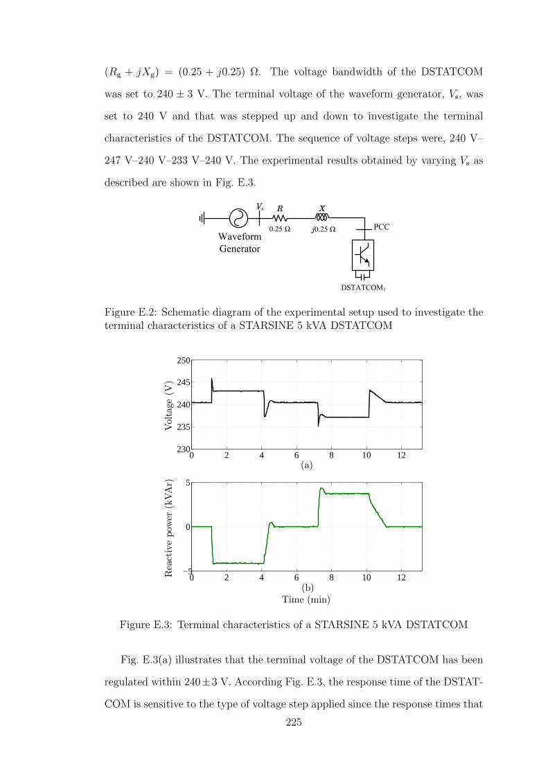
(Rg + jXg) = (0.25 + j0.25) Ω. The voltage bandwidth of the DSTATCOM
was set to 240 ± 3 V. The terminal voltage of the waveform generator, Vs, was
set to 240 V and that was stepped up and down to investigate the terminal
characteristics of the DSTATCOM. The sequence of voltage steps were, 240 V–
247 V–240 V–233 V–240 V. The experimental results obtained by varying Vs as
described are shown in Fig. E.3.
XR
Waveform Generator
DSTATCOM1
0.25 Ω j0.25 Ω PCC
Vs
Figure E.2: Schematic diagram of the experimental setup used to investigate theterminal characteristics of a STARSINE 5 kVA DSTATCOM
0 2 4 6 8 10 12230
235
240
245
250
Voltage
(V)
(a)
0 2 4 6 8 10 12−5
0
5
Reactivepow
er(kVAr)
(b)Time (min)
Figure E.3: Terminal characteristics of a STARSINE 5 kVA DSTATCOM
Fig. E.3(a) illustrates that the terminal voltage of the DSTATCOM has been
regulated within 240±3 V. According Fig. E.3, the response time of the DSTAT-
COM is sensitive to the type of voltage step applied since the response times that
225
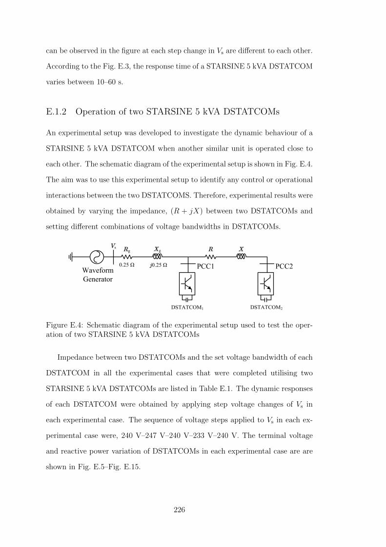
can be observed in the figure at each step change in Vs are different to each other.
According to the Fig. E.3, the response time of a STARSINE 5 kVA DSTATCOM
varies between 10–60 s.
E.1.2 Operation of two STARSINE 5 kVA DSTATCOMs
An experimental setup was developed to investigate the dynamic behaviour of a
STARSINE 5 kVA DSTATCOM when another similar unit is operated close to
each other. The schematic diagram of the experimental setup is shown in Fig. E.4.
The aim was to use this experimental setup to identify any control or operational
interactions between the two DSTATCOMS. Therefore, experimental results were
obtained by varying the impedance, (R + jX) between two DSTATCOMs and
setting different combinations of voltage bandwidths in DSTATCOMs.
XgRg
Waveform Generator
DSTATCOM1
0.25 Ω j0.25 Ω
DSTATCOM2
XRVs
PCC1 PCC2
Figure E.4: Schematic diagram of the experimental setup used to test the oper-ation of two STARSINE 5 kVA DSTATCOMs
Impedance between two DSTATCOMs and the set voltage bandwidth of each
DSTATCOM in all the experimental cases that were completed utilising two
STARSINE 5 kVA DSTATCOMs are listed in Table E.1. The dynamic responses
of each DSTATCOM were obtained by applying step voltage changes of Vs in
each experimental case. The sequence of voltage steps applied to Vs in each ex-
perimental case were, 240 V–247 V–240 V–233 V–240 V. The terminal voltage
and reactive power variation of DSTATCOMs in each experimental case are are
shown in Fig. E.5–Fig. E.15.
226
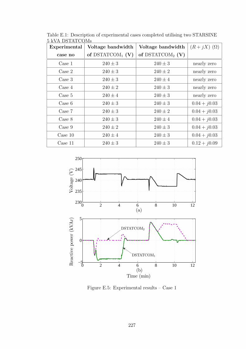
Table E.1: Description of experimental cases completed utilising two STARSINE5 kVA DSTATCOMsExperimental Voltage bandwidth Voltage bandwidth (R + jX) (Ω)
case no of DSTATCOM1 (V) of DSTATCOM2 (V)
Case 1 240± 3 240± 3 nearly zero
Case 2 240± 3 240± 2 nearly zero
Case 3 240± 3 240± 4 nearly zero
Case 4 240± 2 240± 3 nearly zero
Case 5 240± 4 240± 3 nearly zero
Case 6 240± 3 240± 3 0.04 + j0.03
Case 7 240± 3 240± 2 0.04 + j0.03
Case 8 240± 3 240± 4 0.04 + j0.03
Case 9 240± 2 240± 3 0.04 + j0.03
Case 10 240± 4 240± 3 0.04 + j0.03
Case 11 240± 3 240± 3 0.12 + j0.09
0 2 4 6 8 10 12230
235
240
245
250
Voltage
(V)
(a)
0 2 4 6 8 10 12−5
0
5
Reactivepow
er(kVAr)
(b)Time (min)
DSTATCOM1
DSTATCOM2
Figure E.5: Experimental results – Case 1
227
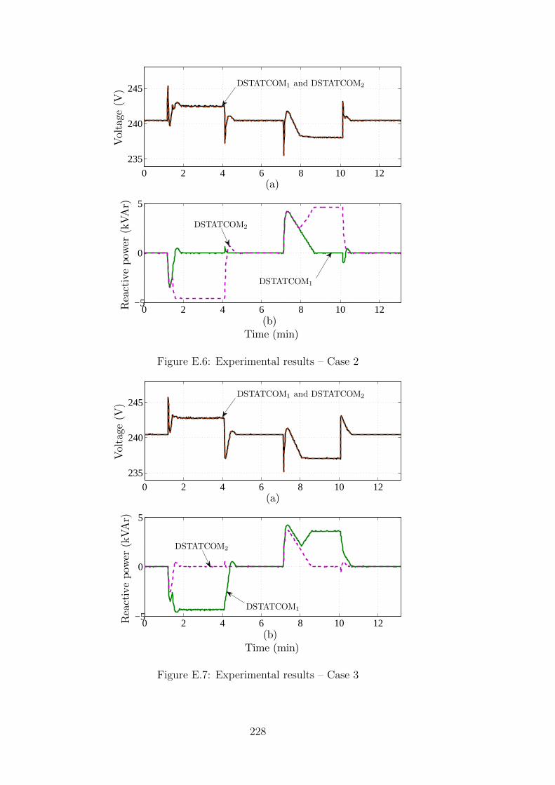
0 2 4 6 8 10 12
235
240
245
Voltage
(V)
(a)
0 2 4 6 8 10 12−5
0
5
Reactivepow
er(kVAr)
(b)Time (min)
DSTATCOM1 and DSTATCOM2
DSTATCOM1
DSTATCOM2
Figure E.6: Experimental results – Case 2
0 2 4 6 8 10 12
235
240
245
Voltage
(V)
(a)
0 2 4 6 8 10 12−5
0
5
Reactivepow
er(kVAr)
(b)Time (min)
DSTATCOM1 and DSTATCOM2
DSTATCOM2
DSTATCOM1
Figure E.7: Experimental results – Case 3
228

0 2 4 6 8 10 12
235
240
245
Voltage
(V)
(a)
0 2 4 6 8 10 12−5
0
5
Reactivepow
er(kVAr)
(b)Time (min)
DSTATCOM1 and DSTATCOM2
DSTATCOM2
DSTATCOM1
Figure E.8: Experimental results – Case 4
0 2 4 6 8 10 12
235
240
245
Voltage
(V)
(a)
0 2 4 6 8 10 12−5
0
5
Reactivepow
er(kVAr)
(b)Time (min)
DSTATCOM1 and DSTATCOM2
DSTATCOM2
DSTATCOM1
Figure E.9: Experimental results – Case 5
229
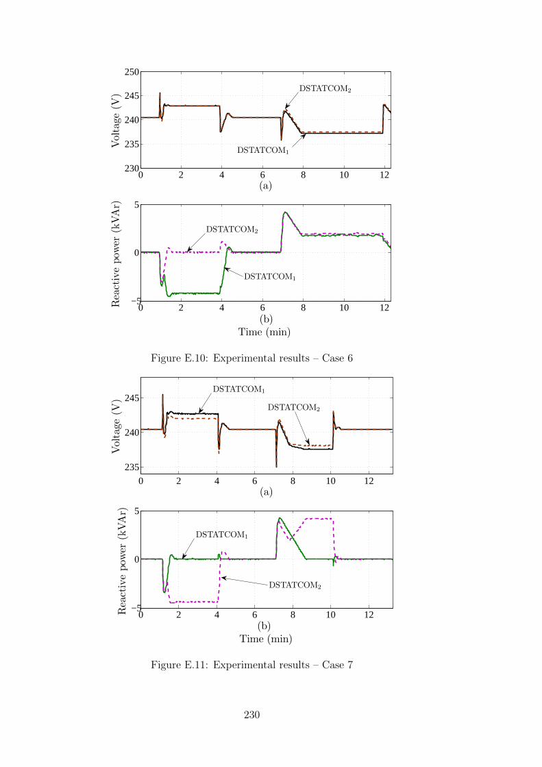
0 2 4 6 8 10 12230
235
240
245
250
Voltage
(V)
(a)
0 2 4 6 8 10 12−5
0
5
Reactivepow
er(kVAr)
(b)Time (min)
DSTATCOM1
DSTATCOM2
DSTATCOM1
DSTATCOM2
Figure E.10: Experimental results – Case 6
0 2 4 6 8 10 12
235
240
245
Voltage
(V)
(a)
0 2 4 6 8 10 12−5
0
5
Reactivepow
er(kVAr)
(b)Time (min)
DSTATCOM1
DSTATCOM1
DSTATCOM2
DSTATCOM2
Figure E.11: Experimental results – Case 7
230
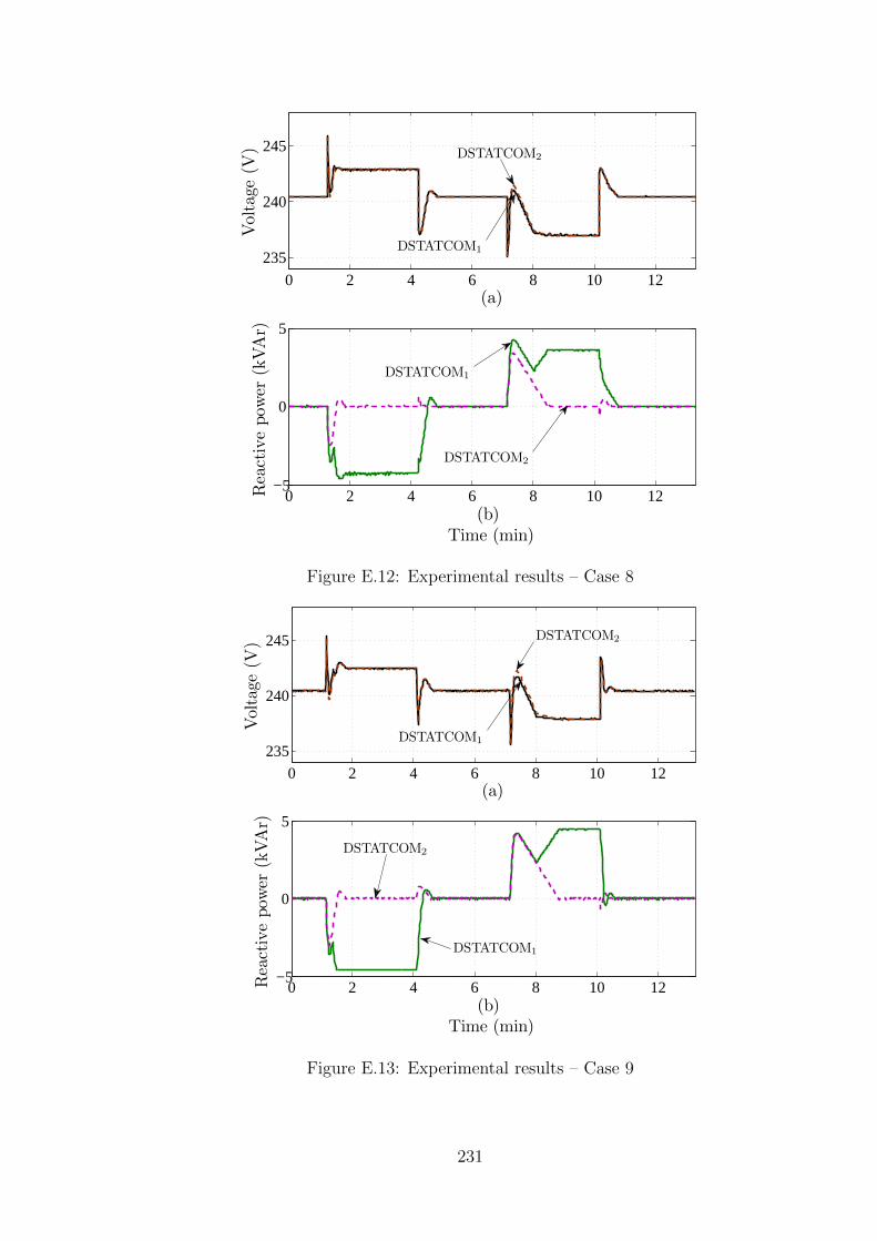
0 2 4 6 8 10 12
235
240
245
Voltage
(V)
(a)
0 2 4 6 8 10 12−5
0
5
Reactivepow
er(kVAr)
(b)Time (min)
DSTATCOM2
DSTATCOM1
DSTATCOM2
DSTATCOM1
Figure E.12: Experimental results – Case 8
0 2 4 6 8 10 12
235
240
245
Voltage
(V)
(a)
0 2 4 6 8 10 12−5
0
5
Reactivepow
er(kVAr)
(b)Time (min)
DSTATCOM1
DSTATCOM2
DSTATCOM1
DSTATCOM2
Figure E.13: Experimental results – Case 9
231

0 2 4 6 8 10 12
235
240
245
Voltage
(V)
(a)
0 2 4 6 8 10 12−5
0
5
Reactivepow
er(kVAr)
(b)Time (min)
DSTATCOM2
DSTATCOM2
DSTATCOM1
DSTATCOM1
Figure E.14: Experimental results – Case 10
0 2 4 6 8 10 12230
235
240
245
250
Voltage
(V)
(a)
0 2 4 6 8 10 12−5
0
5
Reactivepow
er(kVAr)
(b)Time (min)
DSTATCOM1
DSTATCOM1
DSTATCOM2
DSTATCOM2
Figure E.15: Experimental results – Case 11
232
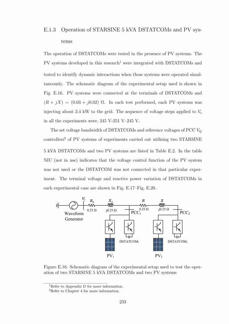
E.1.3 Operation of STARSINE 5 kVA DSTATCOMs and PV sys-
tems
The operation of DSTATCOMs were tested in the presence of PV systems. The
PV systems developed in this research1 were integrated with DSTATCOMs and
tested to identify dynamic interactions when these systems were operated simul-
taneously. The schematic diagram of the experimental setup used is shown in
Fig. E.16. PV systems were connected at the terminals of DSTATCOMs and
(R + jX) = (0.03 + j0.02) Ω. In each test performed, each PV systems was
injecting about 2.4 kW to the grid. The sequence of voltage steps applied to Vs
in all the experiments were, 245 V-251 V–245 V.
The set voltage bandwidth of DSTATCOMs and reference voltages of PCC VQ
controllers2 of PV systems of experiments carried out utilising two STARSINE
5 kVA DSTATCOMs and two PV systems are listed in Table E.2. In the table
NIU (not in use) indicates that the voltage control function of the PV system
was not used or the DSTATCOM was not connected in that particular exper-
iment. The terminal voltage and reactive power variation of DSTATCOMs in
each experimental case are shown in Fig. E.17–Fig. E.20.
XgRg
Waveform Generator
DSTATCOM1
0.25 Ω j0.25 Ω
DSTATCOM2
XRVs
PCC1 PCC2
PV1 PV2
0.25 Ω j0.25 Ω
Figure E.16: Schematic diagram of the experimental setup used to test the oper-ation of two STARSINE 5 kVA DSTATCOMs and two PV systems
1Refer to Appendix D for more information.2Refer to Chapter 4 for more information.
233
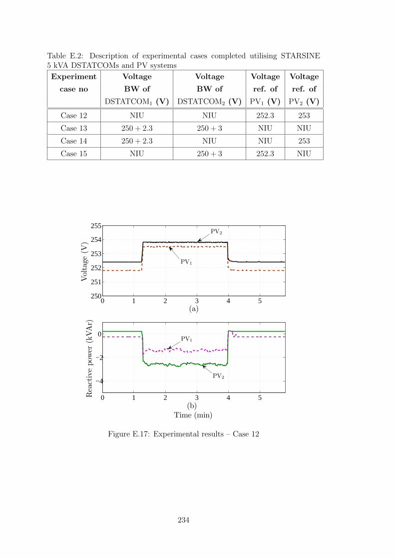
Table E.2: Description of experimental cases completed utilising STARSINE5 kVA DSTATCOMs and PV systems
Experiment Voltage Voltage Voltage Voltage
case no BW of BW of ref. of ref. of
DSTATCOM1 (V) DSTATCOM2 (V) PV1 (V) PV2 (V)
Case 12 NIU NIU 252.3 253
Case 13 250 + 2.3 250 + 3 NIU NIU
Case 14 250 + 2.3 NIU NIU 253
Case 15 NIU 250 + 3 252.3 NIU
0 1 2 3 4 5250
251
252
253
254
255
Voltage
(V)
(a)
0 1 2 3 4 5
−4
−2
0
Reactivepow
er(kVAr)
(b)Time (min)
PV2
PV1
PV1
PV2
Figure E.17: Experimental results – Case 12
234
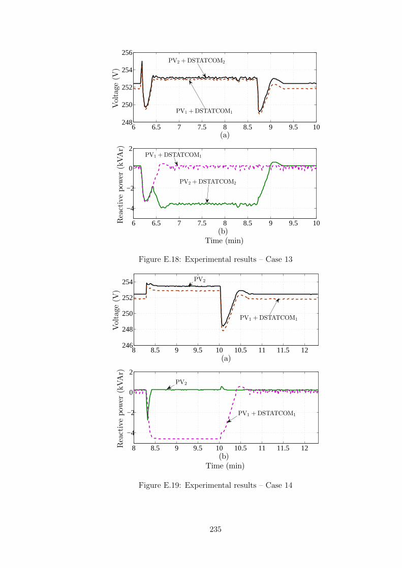
6 6.5 7 7.5 8 8.5 9 9.5 10248
250
252
254
256
Voltage
(V)
(a)
6 6.5 7 7.5 8 8.5 9 9.5 10
−4
−2
0
2
Reactivepow
er(kVAr)
(b)Time (min)
PV2 +DSTATCOM2
PV1 +DSTATCOM1
PV1 +DSTATCOM1
PV2 +DSTATCOM2
Figure E.18: Experimental results – Case 13
8 8.5 9 9.5 10 10.5 11 11.5 12246
248
250
252
254
Voltage
(V)
(a)
8 8.5 9 9.5 10 10.5 11 11.5 12
−4
−2
0
2
Reactivepow
er(kVAr)
(b)Time (min)
PV2
PV2
PV1 +DSTATCOM1
PV1 +DSTATCOM1
Figure E.19: Experimental results – Case 14
235
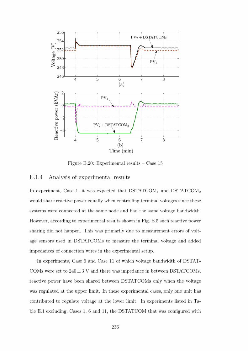
4 5 6 7 8246
248
250
252
254
256
Voltage
(V)
(a)
4 5 6 7 8
−4
−2
0
2
Reactivepow
er(kVAr)
(b)Time (min)
PV2 +DSTATCOM2
PV2 +DSTATCOM2
PV1
PV1
Figure E.20: Experimental results – Case 15
E.1.4 Analysis of experimental results
In experiment, Case 1, it was expected that DSTATCOM1 and DSTATCOM2
would share reactive power equally when controlling terminal voltages since these
systems were connected at the same node and had the same voltage bandwidth.
However, according to experimental results shown in Fig. E.5 such reactive power
sharing did not happen. This was primarily due to measurement errors of volt-
age sensors used in DSTATCOMs to measure the terminal voltage and added
impedances of connection wires in the experimental setup.
In experiments, Case 6 and Case 11 of which voltage bandwidth of DSTAT-
COMs were set to 240±3 V and there was impedance in between DSTATCOMs,
reactive power have been shared between DSTATCOMs only when the voltage
was regulated at the upper limit. In these experimental cases, only one unit has
contributed to regulate voltage at the lower limit. In experiments listed in Ta-
ble E.1 excluding, Cases 1, 6 and 11, the DSTATCOM that was configured with
236
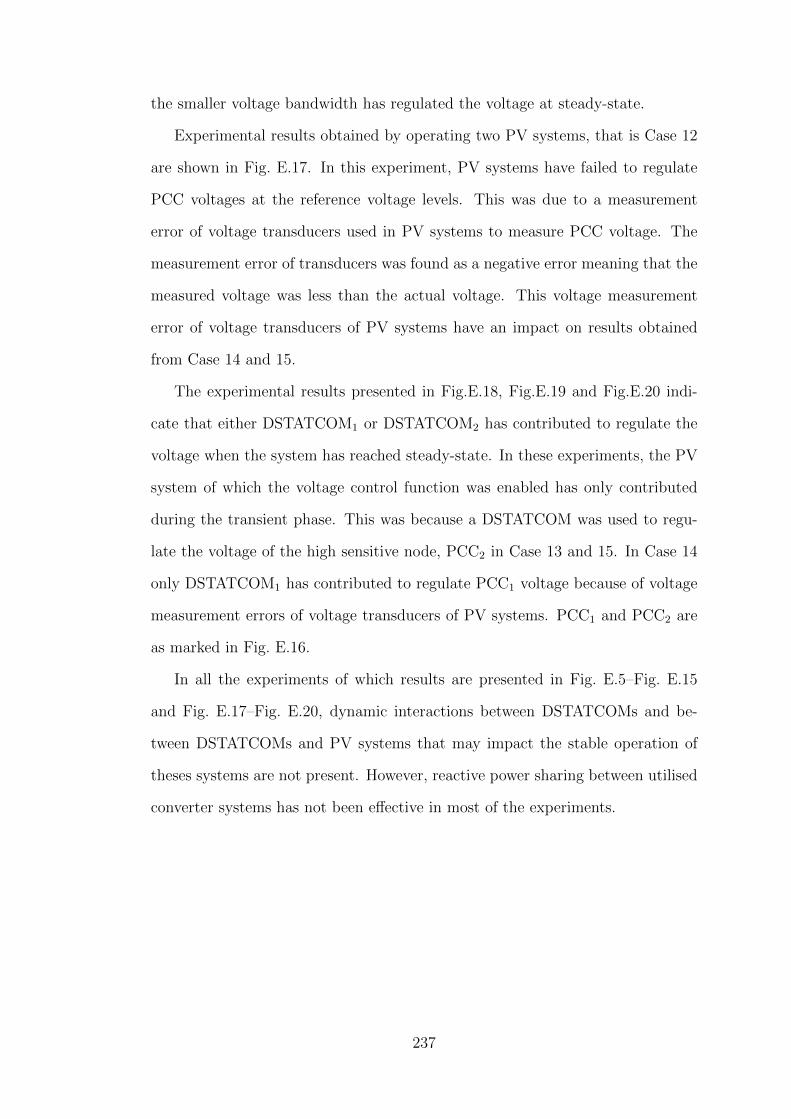
the smaller voltage bandwidth has regulated the voltage at steady-state.
Experimental results obtained by operating two PV systems, that is Case 12
are shown in Fig. E.17. In this experiment, PV systems have failed to regulate
PCC voltages at the reference voltage levels. This was due to a measurement
error of voltage transducers used in PV systems to measure PCC voltage. The
measurement error of transducers was found as a negative error meaning that the
measured voltage was less than the actual voltage. This voltage measurement
error of voltage transducers of PV systems have an impact on results obtained
from Case 14 and 15.
The experimental results presented in Fig.E.18, Fig.E.19 and Fig.E.20 indi-
cate that either DSTATCOM1 or DSTATCOM2 has contributed to regulate the
voltage when the system has reached steady-state. In these experiments, the PV
system of which the voltage control function was enabled has only contributed
during the transient phase. This was because a DSTATCOM was used to regu-
late the voltage of the high sensitive node, PCC2 in Case 13 and 15. In Case 14
only DSTATCOM1 has contributed to regulate PCC1 voltage because of voltage
measurement errors of voltage transducers of PV systems. PCC1 and PCC2 are
as marked in Fig. E.16.
In all the experiments of which results are presented in Fig. E.5–Fig. E.15
and Fig. E.17–Fig. E.20, dynamic interactions between DSTATCOMs and be-
tween DSTATCOMs and PV systems that may impact the stable operation of
theses systems are not present. However, reactive power sharing between utilised
converter systems has not been effective in most of the experiments.
237


![Control of Inverter-Interfaced Distributed Generation ...joape.uma.ac.ir/article_428_11b1f55fc7b1f79a62b2f2ae50109c4b.pdf · In Refs. [7-11], some methods have been presented for](https://img.pdfslide.us/doc/110x75/5fd176ac5dc01a1b367c6142/control-of-inverter-interfaced-distributed-generation-joapeumaacirarticle42811b1f55fc7b1.jpg)


![Inverter-Based Generation Only—An Analysis on Dynamic ......microgrid [6]. Inverter-interfaced energy resources behave completely di erent compared to synchronous generators [7],](https://img.pdfslide.us/doc/110x75/612503dbe636eb70250656b7/inverter-based-generation-onlyaan-analysis-on-dynamic-microgrid-6-inverter-interfaced.jpg)