ISSN 0280-5316ISRN LUTFD2/TFRT—5668—SE

Modelling of a Gas Turbine withModelicaTM

Antonio Alejandro Gómez Pérez

Department of Automatic ControlLund Institute of Technology

May 2001

Document nameMASTER THESISDate of issueMay 2001

Department of Automatic ControlLund Institute of TechnologyBox 118SE-221 00 Lund Sweden Document Number

ISRN LUTFD2/TFRT—5668--SESupervisorsA. Rantzer H. Tummescheit

Author(s)Antonio Alejandro Gómez Pérez

Sponsoring organization

Title and subtitleModeling of a Gas Turbine in Modelica (Modellering av en gasturbin i Modelica)

Abstract

The report describes the development of a global model of a simple gas turbine in order to simulate the dynamic

behaviour. The Modelica language is used for the creation of the model. The model is based on the evaporative gas

turbine located in the Department of Heat and Power Engineering in Lund. This turbine was run as a conventional turbine

before including the heat exchanger and the evaporative tower. The model can be split up in three main parts: the

compressor, the combustion chamber and the expander. These three models are based on the equations obtained from

thermodynamic literature. Furthermore, information provided by the manufacturer was used for the implementation of the

compressor and the expander models. Hence, the thesis is focused first on creating a model of a simple gas turbine by

using as many components of the ThermoFlow library as possible and second on extending the library with reusable

models for turbines and compressors. Since the model involves mechanical parts, components of the rotational sub-library

are used for the task.

KeywordsObject oriented modeling, Reuse, dynamic simulation,

Classification system and/or index terms (if any)

Supplementary bibliographical information

ISSN and key title0280-5316

ISBN

LanguageEnglish

Number of pages77

Security classification

Recipient’s notes

The report may be ordered from the Department of Automatic Control or borrowed through:University Library 2, Box 3, SE-221 00 Lund, SwedenFax +46 46 222 44 22 E-mail ub2@ub2.se

1

Acknowledgements

I want to express my sincere gratitude to everyone who has helped me

during the development of the thesis. I want to give special thanks to:§ My advisor Hubertus Tummeschcheit who has been supporting me with

infinite patience through all my work

§ My Spanish advisor Jose Hernandez Grau, who gave me important

information for the development of the thesis

§ The Ph.D. student Jaime Arriaga, who helped me with many technical

questions

§ Jonas Eborn who helped me with technical questions about the library

§ The professor Alejandrino Gallego, who made it possible to complete my

degree abroad.

§ The Ph.D. student Ines Romero Navarro, who encouraged me to come to

Sweden.

§ My parents Eulogio Gomez Pastor and Juana Perez Ortega, who made

real the dream of finishing my degree in a foreign country

§ To all my mates and friends in Sweden, who made my time away from

home as enjoyable as could be.

2

To my girlfriend Maria,who supported bravely my decision

of coming to Sweden for all this

period. I hope we can enjoy for all

the time that we were separated

3

NOMENCLATURE......................................................................................................................................5

1. INTRODUCTION ....................................................................................................................................7

1.1 BACKGROUND .......................................................................................................................................71.2 OBJECTIVES ...........................................................................................................................................81.3 WHY A DYNAMIC MODEL?....................................................................................................................81.4 PHASES OF THE PROJECT .......................................................................................................................9

2. GAS TURBINES.....................................................................................................................................11

2.1 BASIC DESCRIPTION.............................................................................................................................112.2 EVAPORATIVE GAS TURBINE..............................................................................................................13

3. MODELICA LANGUAGE...................................................................................................................15

3.1 INTRODUCTION....................................................................................................................................153.2 CHARACTERISTICS OF OBJECT-ORIENTED MODELING........................................................................153.3 NON-CAUSAL MODELING...................................................................................................................16

4. THERMOFLOW LIBRARY................................................................................................................17

4.1 INTRODUCTION....................................................................................................................................174.2 BASIC DESIGN IDEAS ..........................................................................................................................18

Control Volumes ...................................................................................................................................19Flow Models .........................................................................................................................................20Medium Models ....................................................................................................................................21State variable transformation ..............................................................................................................22

4.3 SEQUENCE OF CALCULATION IN A DYNAMIC SIMULATION................................................................24

5.COMPRESSOR.......................................................................................................................................26

5.1 INTRODUCTION....................................................................................................................................265.2 GOVERNING EQUATIONS .....................................................................................................................275.3 USE OF THE COMPRESSOR MAP...........................................................................................................335.4 COMPRESSOR MODEL IN MODELICA...................................................................................................40

CorrectedMass1 ...................................................................................................................................40CorrectedMass2 ...................................................................................................................................40P_maxeff ...............................................................................................................................................40Maxeff....................................................................................................................................................40Efficiency ..............................................................................................................................................40CompressorMap ...................................................................................................................................41IsentropicVariables ..............................................................................................................................41FlowModelBaseMD .............................................................................................................................41PolytropicEfficiency .............................................................................................................................42Compressor ...........................................................................................................................................42CompressorMec....................................................................................................................................42CompleteCompressor ...........................................................................................................................43

6.TURBINE..................................................................................................................................................44

6.1 GOVERNING EQUATIONS .....................................................................................................................446.2 TURBINE MAP ......................................................................................................................................476.3 TURBINE MODEL IN MODELICA ..........................................................................................................49

FlowModelBaseDM .............................................................................................................................49IsentropicVariables ..............................................................................................................................49PolytropicEfficiency .............................................................................................................................49Turbine..................................................................................................................................................50TurbineMec...........................................................................................................................................50CompleteTurbine..................................................................................................................................51

4

7.COMBUSTION CHAMBER.................................................................................................................52

7.1 INTRODUCTION....................................................................................................................................52Mass balance ........................................................................................................................................53Energy Balance ....................................................................................................................................55

7.3 COMBUSTION CHAMBER MODEL IN MODELICA .................................................................................58MassBalance.........................................................................................................................................58Valve......................................................................................................................................................58NaturalGasResS_pTX ..........................................................................................................................58ThreePort ..............................................................................................................................................59CombustionChamber ...........................................................................................................................59

8. TESTING MODELS OF THE TURBINE .........................................................................................60

8.1 SYSTEM MODEL WITH HYDRAULIC BRAKE.........................................................................................608.2 SYSTEM MODEL WITH SPEED CONTROLLER........................................................................................62

9.SIMULATION RESULTS .....................................................................................................................63

9.1 SIMULATION IN THE MODEL WITH HYDRAULIC BRAKE......................................................................639.2 SIMULATION OF THE MODEL WITH SPEED CONTROLLER...................................................................72

10. CONCLUSIONS AND FUTURE WORK........................................................................................75

10.1 CONCLUSIONS ...................................................................................................................................7510.2 FUTURE WORK...................................................................................................................................75

BIBLIOGRAPHY.......................................................................................................................................76

5

Nomenclature

Symbol Unit Physical Meaning

A m2 surface area

c J/(kgK) specific heat capacity

F N axial force

h J/kg specific enthalpy

I kgm/s axial momentum

J - Jacobean matrix

m kg/s mass flow rate

M kg mass

n rpm rotational speed

p Pa pressure

P W power

q J/kg heat flow

Q J/s heat flow

R J/(molK) universal gas constant

s J/(kgK) specific entropy

t s time

T K temperature

u J/kg specific internal energy

U J internal energy

6

v m3/kg specific volume

V m3 volume

w kg/mol molecular weight

w J/kg specific work

γ - ratio of specific heats

η - efficiency

ρ kg/m3 density

τ Nm torque

ω rad/s rotational speed

U J internal energy

7

1. Introduction

1.1 Background

Due to the wide range of interactions between different engineering fields,

systems are getting more complex and heterogeneous. When trying to create models

of these systems, problems arise with the interaction of the different parts. Many

times, it is possible to find simulation programs with graphical user interfaces for

creating complex model. The main problem using these interfaces is that they are

normally very specific, and are constrained to a concrete engineering discipline.

Some examples of this kind of programs are Spice and Saber for electronics

simulations, or ASPEN Plus and SpeedUp for simulation of chemical processes.

Therefore, they are not appropriate when dealing with interoperatibily in

heterogeneous problems.

Among the recent research results in modelling and simulation, two concepts

have strong relevance to this problem:

§ Object oriented modelling languages have demonstrated how object

oriented concepts can be successfully employed to support hierarchical

structuring, reuse and evolution of large and complex models,

independent from the application domain and specialised graphical

formalisms. By using these languages, it is possible to support modularity

on multiple levels. It means that a model can have many submodels,

which have submodels themselves.

§ Non-causal modeling. The traditional approach for simulation based on

input and output blocks, is replaced by another one where interaction is

not defined with inputs or outputs. This generalisation provides both

simpler models and more efficient simulations, while retaining the

capability to include submodels with fixed input output relations.

During the last four years the object-oriented, multi-domain language

Modelica has been developed by an international group of engineers and

researchers. The goal of the Modelica design is to become a de-facto standard for

physical modeling languages. Another activity of the group is to also develop basic,

free model libraries for several applications domains. The library for thermo-hydraulic

8

processes is currently being developed at the Department of Automatic Control,

Lund.

A base library like the one in progress in Lund can only prove its usefulness in

practical applications with industrial relevance. Hence, the thesis is focused first on

creating a model of a simple gas turbine by using as many components of the

ThermoFlow library as possible and second on extending the library with reusable

models for turbines and compressors. Since the model involves mechanical parts,

components of the rotational sub-library are used for the task. This project is

performed in close cooperation with the Department of Heat and Power Engineering,

which runs a pilot plant for an evaporative gas turbine at Lund University.

1.2 Objectives

The objective of this thesis is to develop a global model of a simple gas

turbine in order to simulate the dynamic behaviour. The Modelica language is used

for the creation of the model. The model is based on the evaporative gas turbine

located in the Department of Heat and Power Engineering in Lund (Lindquist, 1999).

This turbine was run as a conventional turbine before including the heat exchanger

and the evaporative tower. Due to the large quantity of parameters involved in the

model, the goal is to reproduce the general dynamic behaviour of the turbine. It

should be noted that the approximation in the result obtained the model and the

results obtained with the experiments depend on many model parameters. The

tuning of the parameters of the model is beyond the scope the project.

The model can be split up in three main parts: the compressor, the

combustion chamber and the expander. These three models are based on the

equations obtained from thermodynamic literature, mainly in (Cohen, 1996), (Cengel,

1994) and (Philips, 1999). Furthermore, information provided by the manufacturer

was used for the implementation of the compressor and the expander models.

A model of a hydraulic brake or another kind of power sink needs to be

implemented in order to extract power from the turbine. The models of compressor,

expander and brake are mechanically coupled.

1.3 Why a dynamic model?

When designing a gas turbine for generating electrical power, the most

important thing is to obtain a high efficiency of the system. Therefore, an operating

9

point is chosen, and all calculations are based on this design point. Static models are

normally used for the design of gas turbines. However, it is not possible to know the

response of the plant during transients by using static models. A concrete case of a

transient can be a change in the requested power. It is known that in a gas turbine

the highest temperature in the cycle is reached at the end of the combustion

chamber, before the turbine, which is approximately the same than at the inlet of the

expander. The maximum temperature that the turbine blades can withstand limits the

turbine inlet temperature (TIT). Therefore, the maximum pressure ratio that can be

used in the cycle is also limited, because the TIT is associated to this pressure ratio.

Increasing the turbine inlet temperature has been one of the main approaches to

improve the gas turbine efficiency. The development of new materials and new

cooling techniques has made possible the increase of the TIT. This development has

also resulted in more expensive components and the necessity of controlling that

these components are working in the right operating range. Consequently, it is

necessary to evaluate the behaviour of the plant during different transients in order to

keep the TIT in the right range. Dynamic models are used for addressing questions

like this.

It should be noted that these models are more complicated than the static

models, and it could yield problems for evaluating the equations of the model. Hence,

the models have to be simple and at the same time accurate enough for the

simulations. Dynamic models are used mainly in order to control the plant. These

models can be used for simulating different parts of the plant and to plug them

together, for analysing the behaviour of the whole plant. Then, new controllers can be

tested improving the global behaviour of the turbine. Another important function of

the dynamic models is the training of the personal in power plant. Dynamics models

are created to reproduce the behaviour of the plant. In this way, the staff of the

company can be prepared by using simulation based on these models.

1.4 Phases of the project

The project was divided in the following phases:

§ Study of the features of the language Modelica

§ Study of the structure and models in the ThermoFlow library

10

§ Study of the governing equations and technical data for the main parts of

the plant.

§ Development and implementation of the different models of the plant

§ Simulation of the global model of the turbine

§ Discussion of the results obtained in the simulations

11

2. Gas Turbines

2.1 Basic description

It is known that nowadays, all the society in general is dependent on the

electrical power. Most of generation of heat and power is dominated by the use of

fossil fuels. Turbines are the main devices for generating electrical power by using

these fuels. There are basically two kinds of turbines: steam and gas turbines. Steam

turbines are able to generate larger power than gas turbines and with an overall

efficiency over 40%, but they have the drawback that rather complicated installations

for generating steam are needed. On the other hand, gas turbines are much more

compact power plants than steam turbines, since steam does not need to be

generated and hot gases are used directly to run the turbine. Therefore, gas turbines

have very short start-up times.

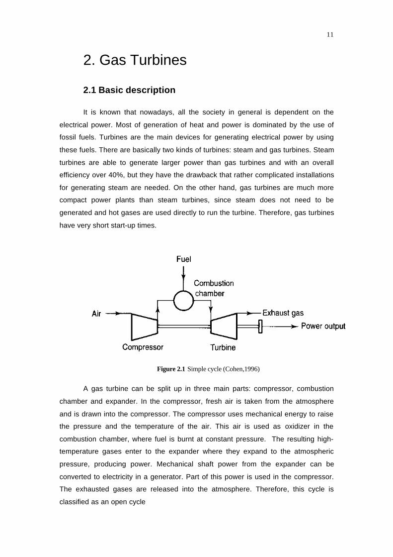
Figure 2.1 Simple cycle (Cohen,1996)

A gas turbine can be split up in three main parts: compressor, combustion

chamber and expander. In the compressor, fresh air is taken from the atmosphere

and is drawn into the compressor. The compressor uses mechanical energy to raise

the pressure and the temperature of the air. This air is used as oxidizer in the

combustion chamber, where fuel is burnt at constant pressure. The resulting high-

temperature gases enter to the expander where they expand to the atmospheric

pressure, producing power. Mechanical shaft power from the expander can be

converted to electricity in a generator. Part of this power is used in the compressor.

The exhausted gases are released into the atmosphere. Therefore, this cycle is

classified as an open cycle

12

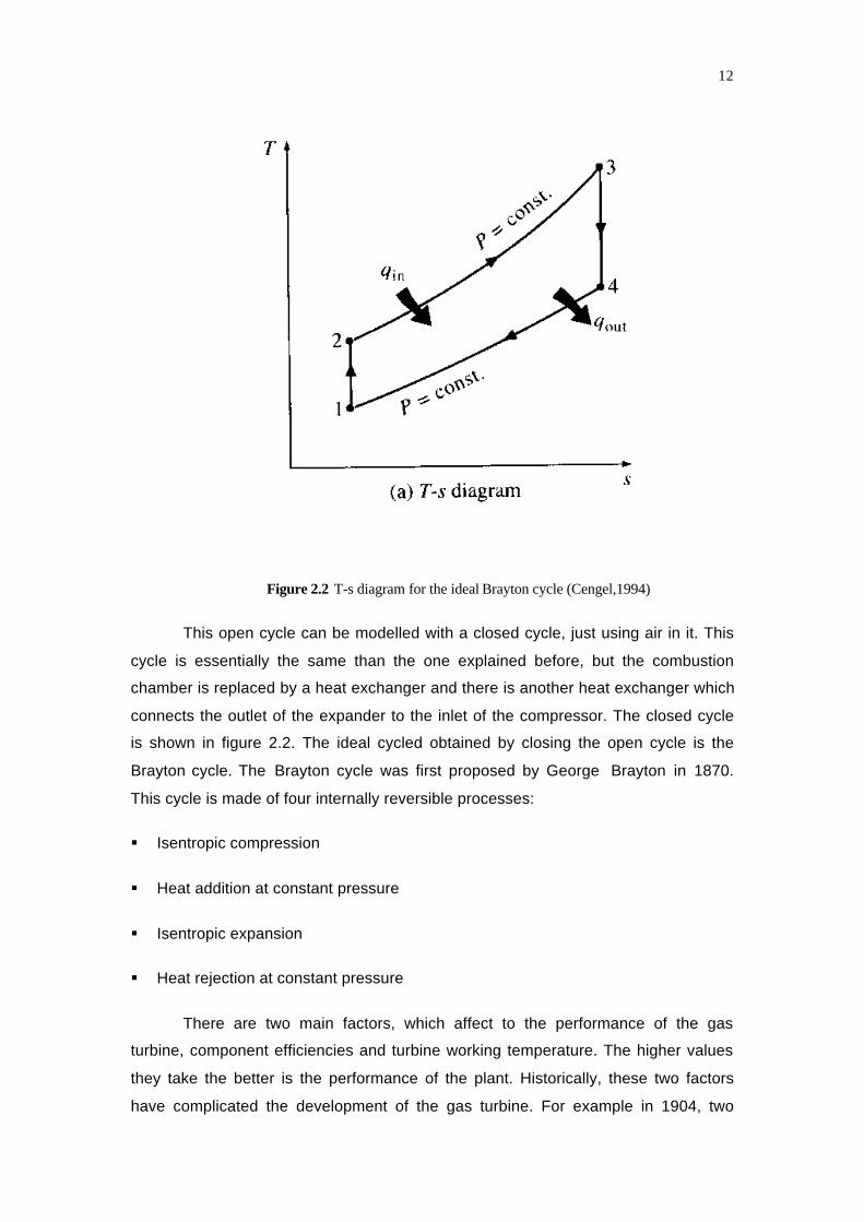
Figure 2.2 T-s diagram for the ideal Brayton cycle (Cengel,1994)

This open cycle can be modelled with a closed cycle, just using air in it. This

cycle is essentially the same than the one explained before, but the combustion

chamber is replaced by a heat exchanger and there is another heat exchanger which

connects the outlet of the expander to the inlet of the compressor. The closed cycle

is shown in figure 2.2. The ideal cycled obtained by closing the open cycle is the

Brayton cycle. The Brayton cycle was first proposed by George Brayton in 1870.

This cycle is made of four internally reversible processes:

§ Isentropic compression

§ Heat addition at constant pressure

§ Isentropic expansion

§ Heat rejection at constant pressure

There are two main factors, which affect to the performance of the gas

turbine, component efficiencies and turbine working temperature. The higher values

they take the better is the performance of the plant. Historically, these two factors

have complicated the development of the gas turbine. For example in 1904, two

13

French engineers, Armegaud and Lemale, made a turbine, which could hardly turn

itself. It was due to the low efficiency in the compressor, around 60%, and the

limitation of the gas temperature, around 740 K. Nowadays, the efficiencies of the

components are around 85-90% and the temperatures that the turbines can

withstand exceed 1650 K.

2.2 Evaporative Gas Turbine

The evaporative gas turbine developed at the Department of Heat and Power

Engineering in Lund is briefly described in this section.

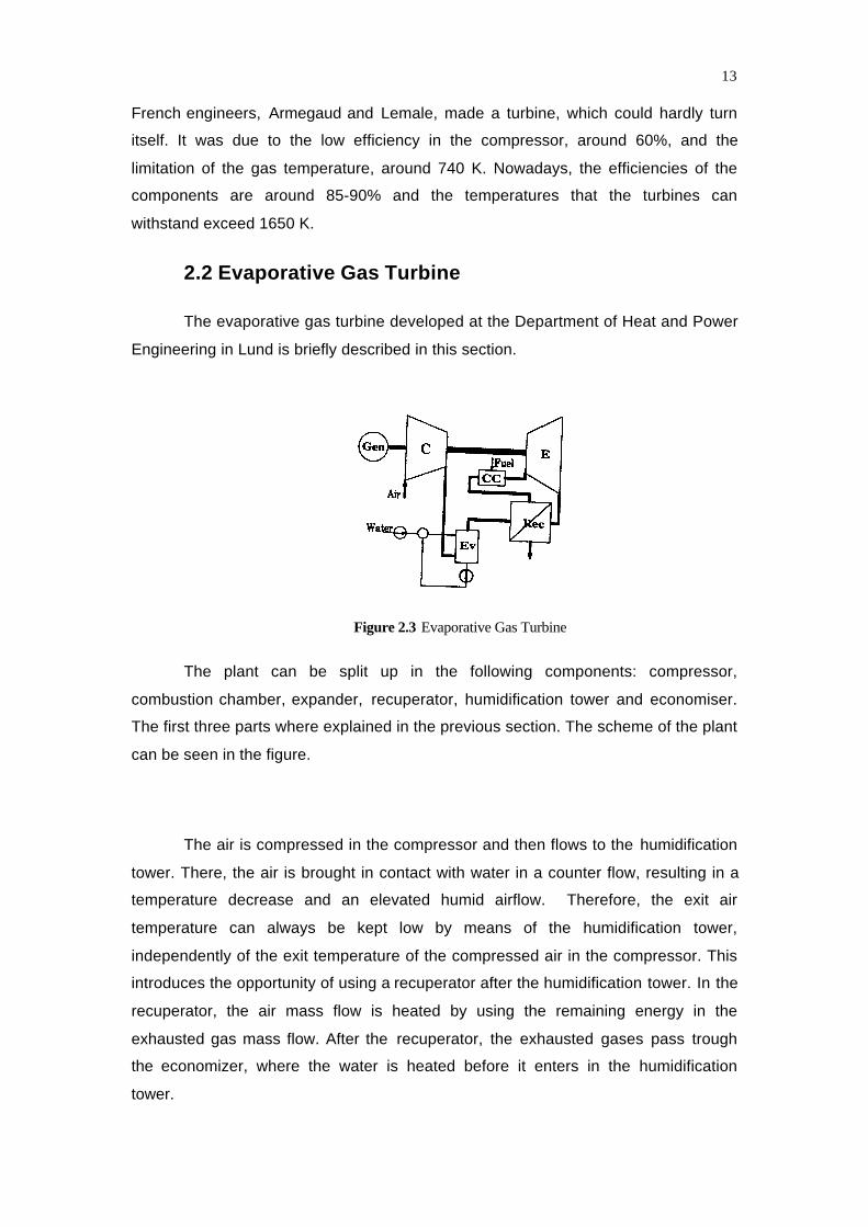
Figure 2.3 Evaporative Gas Turbine

The plant can be split up in the following components: compressor,

combustion chamber, expander, recuperator, humidification tower and economiser.

The first three parts where explained in the previous section. The scheme of the plant

can be seen in the figure.

The air is compressed in the compressor and then flows to the humidification

tower. There, the air is brought in contact with water in a counter flow, resulting in a

temperature decrease and an elevated humid airflow. Therefore, the exit air

temperature can always be kept low by means of the humidification tower,

independently of the exit temperature of the compressed air in the compressor. This

introduces the opportunity of using a recuperator after the humidification tower. In the

recuperator, the air mass flow is heated by using the remaining energy in the

exhausted gas mass flow. After the recuperator, the exhausted gases pass trough

the economizer, where the water is heated before it enters in the humidification

tower.

14

Tests carried out in the pilot plant showed that the efficiency increased from

22.27% in the simple cycle to 35% in the evaporative cycle. The NOx emissions were

reduced by 90% to under 10 ppm, and the UHC (uncombusted hydro carbons) and

CO were not measurable when running the evaporative cycle at rated power output.

Other advantages of the plant are that it is possible to reach full power output in less

than five minutes and the investment costs for the evaporative cycle are much

smaller than for other cycles with the same efficiency. More information about the

EvGT can be found in (Lindquist,1999).

15

3. Modelica language

3.1 Introduction

Modelica is an object-oriented language developed for creating large,

complex and heterogeneous physical problems. General equations are used for

modelling the physical phenomena. No particular variable needs to be solved for

manually, since the Modelica tool will have enough information to do that

automatically. Object-oriented and non-causal are important concepts in Modelica.

Both concepts are sometimes confused. The concept of object-oriented refers to the

structuring of the models whereas the concept of non-causal refers to the underlying

description of the behaviour of the models. Nevertheless, these concepts are used

together in constrast to the traditional concept based in block-oriented models, which

comes more from concern with computational aspects than from user concerns. The

Modelica language relies on these concepts of object-oriented and non-causal

model. In this chapter some general ideas about these two notions are given.

3.2 Characteristics of object-oriented modeling

The principal point is that object-oriented modelling is able to study a system

as a set of interacting objects. The total system is decomposed into simpler

elements, which are easier to study. Each object encapsulates data, behaviour and

structure. Once each object is defined, it is necessary to define the different

connections for these objects and finally their behaviour. With these simple units it is

possible to build models and submodels in an easy way. Models define facts and

relations, rather that being procedures for computing data. In object-oriented

modelling the models are treated as objects. These objects are described by a class,

which can be seen as a blue-print of the model. A model representation must support

modularity on multiple levels, which means that one model can have many

submodels which have submodels themselves. A model is also studied as something

abstract, which means that it can be used without knowing all the details about its

definition. In an abstract model, it is possible to speak about an interface and internal

description. The interface of the model describes how the variables that are internal

to the model interact with the environment. The part of the model that has no

interaction with the environment is the internal definition.

16

3.3 Non-Causal Modeling

In order to allow reuse of components models, the equations should be stated

in a neutral form without consideration of computational order, i.e. non-causal

modeling. Most of the general-purpose simulation softwares on the market assume

that the systems have to be split up into block diagrams structures. Therefore, these

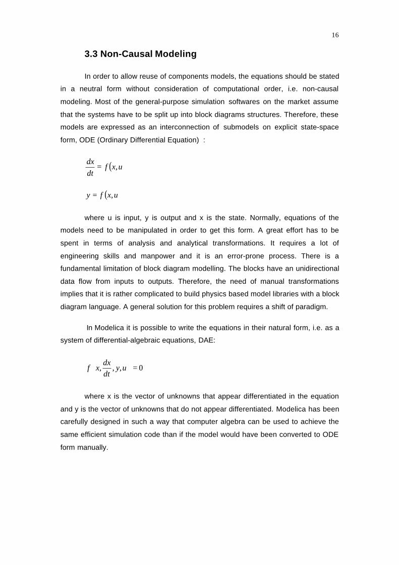
models are expressed as an interconnection of submodels on explicit state-space

form, ODE (Ordinary Differential Equation) :

( )uxfdtdx

,=

( )uxfy ,=

where u is input, y is output and x is the state. Normally, equations of the

models need to be manipulated in order to get this form. A great effort has to be

spent in terms of analysis and analytical transformations. It requires a lot of

engineering skills and manpower and it is an error-prone process. There is a

fundamental limitation of block diagram modelling. The blocks have an unidirectional

data flow from inputs to outputs. Therefore, the need of manual transformations

implies that it is rather complicated to build physics based model libraries with a block

diagram language. A general solution for this problem requires a shift of paradigm.

In Modelica it is possible to write the equations in their natural form, i.e. as a

system of differential-algebraic equations, DAE:

0,,, =

uy

dtdx

xf

where x is the vector of unknowns that appear differentiated in the equation

and y is the vector of unknowns that do not appear differentiated. Modelica has been

carefully designed in such a way that computer algebra can be used to achieve the

same efficient simulation code than if the model would have been converted to ODE

form manually.

17

4. ThermoFlow library

For creating the complete model of the gas turbine, the ThermoFlow library

was used. The library is under development at the Department of Automatic Control

at the Lund University. This chapter is dedicated to briefly describe the library, in

order to give an idea of how it is used. Further information about the library can be

obtained at www.control.lth.se/~hubertus/ThermoFluid.

4.1 Introduction

Since the range of different thermo-hydraulic applications is very wide, it is

not feasible to try to create complete models for all these applications. When creating

a library to use in these applications, emphasis has to be put in the construction of

reusable models. Therefore, the ThermoFlow library is designed to provide

extensibility of basic building blocks rather than for creating complete models for

specific applications. In this way, the user of the library can combine several of these

basic models to obtain a complete one in a certain application. The basic physics of

flows, fluids and heat need to be covered by the library. Complete physical properties

for different mediums are also needed. For this reason a great effort is put to develop

basic flow models and control volumes. In the control volume is possible to choose

the suitable property model for the desired application. The models in the library are

designed for system level simulation, not for detailed simulation. The models are thus

discretized in one dimension or even lump parameter approximations

The Thermo-Flow library follows basically the following guidelines:

§ One unified library both for lumped and distributed models

§ Separation of the medium submodels, which can be selected through

class parameters

§ Both bi and unidirectional flows are supported

§ Assumptions can be selected through class parameter

The main idea of the library is to enable the user to create complex models

based on the simple models provided.

18

4.2 Basic Design Ideas

A large number of engineering problems involve mass flow in and out of the

system. In many books in thermodynamics these systems are modeled as control

volumes. Inside the control volumes, energy and mass flow are set. In the

ThermoFlow library, control volumes are the basic entity. But another model is

necessary for calculating the mass flow and the convective energy associated to the

mass flow. Because of this, flow models are introduced. A flow model is the result of

a modeling abstraction, where the volume is neglected. These flow models contain

either an algebraic equation that relates pressure drop and mass flow, or an

expression for the dynamic momentum balance. The ThermoFlow library is based on

an alternating sequence of control volumes and flow models. It can be said that

storage of mass and energy are modeled in the control volume, whereas the flow of

mass and energy are modeled in the flow models. Control volumes and flow models

are connected through flow connectors. The flow connector for a single medium flow

without dynamic momentum balance contains the following variables:

{p, h, m, qc, ρ, T, s, k}

where the quantities are pressure, specific enthalpy, mass flow, convective

heat flow, density, temperature, specific entropy and ratio of specific heat,

respectively. All the information for the mass and energy balance is contained in the

variables m and qc, which are evaluated in the flow model. The rest of variables (p, h,

ρ, T, s, k) are evaluated in the control volume.

Figure 4.1 Interaction between CV and FM

19

In order to build up new models using the library it is very important to

understand these two basic models, the control volume and the flow model.

Control Volumes

Control volumes are in fact one of the most important “pillars” of the

ThermoFlow library. As it was said before, a control volume contains energy and

mass balances. But it is also necessary to include a model for calculating all the

thermophysical properties, which is called medium model. The user can choose the

medium model depending on the application. Control volumes contain also

connectors, which are the links between the control volume and the environment.

Through the connectors, the control volume interacts with the rest of the system.

There are two different kinds of connectors:

§ Flow connectors, which were already explained above.

§ Heat transfer connectors. In this connectors there is no mass flow.

These connectors are used for modeling heat transfer between fluids and

solid bodies.

Figure 4.2 Control Volume

Once the connectors have been defined, mass and energy balances in the

control volume can be written as:

( ) ∑=n

inmM

dtd

(4.1)

20

( ) ∑∑ +=l

ijtransfer

n

iiconv qqU

dtd

,

.

,

.

(4.2)

Where M is the total mass, U the total inner energy, n is the number of flow

connections (associated to mass flow m and heat flow qconv) and l the number of heat

transfer connectors (associated to heat transfer qtran). Positive sign is associated to

flows into the control volume. For simplicity, pressure volume work and dissipative

work have been neglected here.

Flow Models

Two volumes have to be connected with a flow model, which contains mainly

the momentum balance. In the ThermoFlow library, two types of flow models are

defined:

§ Stationary pressure drop models.

§ Dynamic momentum balances for pipes with constant cross-sectional

area.

The user can choose the type of flow model to use depending on the model

that he wants to create. It should be kept in mind that the dynamic momentum

balance is only of interest when fast wave dynamics of the system are of interest.

When the main interest is in the thermal behaviour, the stationary pressure drop

should be used.

Figure 4.3 Flow Model

The momentum equation for a pipe with a constant cross-section area and

with volume V is:

21

∫ ∫ ∫∆

∆⋅=⋅⋅⋅=⋅⋅=V z A

zmdzdAwdVwI.

ρρ (4.3)

Where w is the velocity in z direction, A is the normal flow area and m is the

mass flow. Using Newton’s law with only pressure and friction forces acting on the

CV :

( ) wallFAppIIdtdI

dtmdz −⋅−+−==∆ 212

.

1

..

(4.4)

The equation can be simplified in order to obtain a stationary pressure drop

model:

( ) wallFApp −⋅−= 210 (4.5)

Where Fwall is the friction between the fluid and the wall. It depends on the

flow characteristics. Different expressions for Fwall can be found in the literature.

When creating models like a compressor for example, there are many

different relationships between mass flow rate, pressure ratio, angular speed, etc.

Then the flow model can contain these expressions instead of the dynamic

momentum equation.

Medium Models

It is important to have accurate medium models in order to make the library

really reusable. On the other hand, for the purpose of dynamic simulations, it is also

important to have fast medium models. At the moment, the following medium models

are implemented:

§ Pure Ideal gases

§ Mixture of ideal gases

§ CO2

§ Water

The models implemented in the library are all very accurate and are taken

from some recommended formulations or standards like IAPWS/IF97 for water.

22

Medium models are necessary in control volumes. By using this medium models it is

possible to compute all remaining variables of interest using the mass and energy

balances.

State variable transformation

Mass and energy balances are implemented in the control volume model.

Total mass and internal energy (M and U) are the states in these equations. For

using the medium models provided in the library, these variables are not very

suitable. Different variables are chosen as states depending on the choice of the

medium model used. When working with ideal gases, which are used for the turbine

model, p and T are chosen as states, mainly for efficiency reasons. In ideal gases, all

medium properties depend on T. Hence, if h were chosen as a state, there would

always be a non-linear system of equations for calculating T. Because of this there is

a special class in the library called StateTransformation, which changes the states M

and U to different states according to the desired model.

A differentiation of M = ρV and U = uM for a constant volume yields:

dtdM

dtd

V =ρ

(4.6)

dtdM

udtdU

dtdu

M −= (4.7)

So the energy and mass balances described above can be rewritten as:

=

udt

du

VUM

dtd ρ

ρ01

(4.8)

Where ρ is the density and u is the specific inner energy. These primary

equations are then transformed into secondary forms to give differential equations in

the states that are best suited for the medium model. For the case of perfect gases, p

and T are chosen as states. For simplicity, the composition of the gas is assumed

constant, so it is not considered in the transformation:

=

Tp

dTd

Tu

pu

Tpudt

d

pT

pT

δδ

δδ

δδρ

δδρ

ρ(4.9)

23

Where:

=

pT

pT

Tu

pu

TpJ

δδ

δδ

δδρ

δδρ

(4.10)

And for ideal gases:

TRp T ⋅=

1δδρ

(4.11)

2TRp

T p ⋅−=

δδρ

(4.12)

0=Tp

uδδ

(4.13)

vp

CTu

=δδ

(4.14)

To obtain differential equations for pressure and temperature, the following

expression is used:

=

−

udtd

JTp

dtd ρ1 (4.15)

The inverse of the Jacobian is computed as follows:

−

−⋅=−

TT

pp

ppu

TTu

JJ

δδρ

δδ

δδρ

δδ

det11 (4.16)

An the determinant is:

TRC

TRp

TRC

pu

TpTuJ v

vTpTp ⋅

=⋅

⋅−−

⋅⋅=⋅−⋅= 01det 2δ

δδδρ

δδρ

δδ

(4.17)

So the inverse of the Jacobian can be rewritten as:

24

⋅

⋅⋅⋅

=−

TR

TRpC

TRC

Jv

v

10

21 (4.18)

Similar expressions are also implemented in the Library for other pairs of

state variables, for example (p,h), (ρ,T), (ρ,T,x),...where x refers to the composition of

a mixture of gases.

4.3 Sequence of calculation in a dynamic simulation

Once control volumes have been presented, a brief explanation of the way of

operating is given. Pressure and temperature are assumed to be the states. It should

be noted that this sequence of calculation is determined automatically by the Dymola

tool, without any help from the user

§ First of all, initial values of the states pressure and temperature (p0 and

T0) are needed. The user has to supply these values.

§ Knowing the temperature, it is possible to evaluate other termodynamical

variables ( h, ρ, s, k) by using the medium model.

§ The flow models use the value of these variables for evaluating the mass

and energy flows. The flow model accesses this information through the

connectors.

§ All the mass and energy flows calculated in the flow models surrounding

the control volume, are used in the mass and energy balances. Time

derivatives of total mass and total inner energy are then calculated (dM,

dU).

§ The class StateTransformation is used to transform the time derivatives of

total mass and inner energy (dM, dU) into the time derivatives of the

chosen states (dp, dT).

§ The time derivative of pressure and temperature are used for evaluating

the new values of the states. The sequence is repeated again.

The sequence can be seen in the figure.

25

Figure 4.4 Sequence of calculation

26

5.Compressor

5.1 Introduction

The compressor for gases has the same function that the pump for liquids.

Basically, mechanical energy is added to the gases and this is used to raise the

pressure, hence the name compressor. This adding of energy causes the gases to

flow from one unit operation to the next. A compressor is the same than a turbine in

reverse, compressing rather than expanding the gases that pass through it.

The model created for the compressor is based on the general equation for

steady state flow. In this way, faster dynamics are neglected, and replaced by static

relationships. This approach is used when a model has some fast and some slow

dynamics. Higher frequency transients can be neglected, since the low frequency

transients dominate the response. When this assumption is used, it is possible to

base a model on steady state data. A compressor map is used in the compressor

model. By using this map, the polytropic efficiency and the mass flow can be

calculated as functions of the pressure ratio and the rotor speed. The compressor

model includes equation for the mechanical behaviour. Inside the model, mechanical

and thermodynamic powers are connected in an equation.

During the first part of the chapter, the governing equations are explained. In

the second part, the way of implementing the compressor map is shown. Finally, a

short description about the Modelica models created for the compressor is given.

27

5.2 Governing equations

First of all, a steady state energy balance is used. This equation can be found

in many books of thermodynamics (Philip, 1999),( Cengel, 1996):

0=−−−− gdzcdcdhdwdq (5.1)

where the dq is the specific external heating, dw is the specific work, dh is the

enthalpy, cdc is the kinetic energy term and gdz the potential energy term. Normally

a compressor can be considered as adiabatic, so the term dq can be neglected. The

same consideration can be taken for the height difference, so that dz=0. There is a

small difference between the inlet and the outlet velocities, but it can be also

neglected, i.e. cdc=0, (Philip, 1996). According to this, the equation obtained is:

dhdw =− (5.2)

And integrating over the compressor section gives:

12 hhw −=− (5.3)

Where the subscripts 1 and 2 refer to the input and the output sections of the

compressor respectively, and w is the specific work done on the gas. From the

definition of constant specific heat cp(T), for ideal gases, equation (5.3) can be

rewritten as:

( )dTTcw p∫=−2

1

(5.4)

where cp(T) is a function of the temperature. In the Figure (5.1) is possible to

see the variation of cp(T) with the temperature for different gases. For the case of air,

the variation of specific heat with the temperature is smooth, and may be

approximated as linear over intervals of a few hundred degrees, (Cengel, 1994).

Then, the specific heat in equation (5.4) can be replaced by a constant average

specific heat value. An approach is to take the average for the temperatures at

compressor inlet an outlet.

28

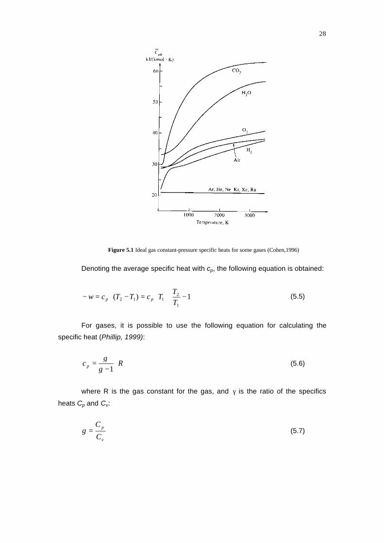
Figure 5.1 Ideal gas constant-pressure specific heats for some gases (Cohen,1996)

Denoting the average specific heat with cp, the following equation is obtained:

−⋅⋅=−⋅=− 1)(

1

2112 T

TTcTTcw pp (5.5)

For gases, it is possible to use the following equation for calculating the

specific heat (Phillip, 1999):

Rc p ⋅−

=1γ

γ(5.6)

where R is the gas constant for the gas, and γ is the ratio of the specifics

heats Cp and Cv:

v

p

C

C=γ (5.7)

29

The specific heat ratio also varies with the temperature, but this variation is

very small. For the case of air, the value of the specific heat ratio is around 1.4

(Cengel,1996). The equation (5.5) can be rewritten as:

−⋅⋅⋅

−=− 1

1 1

21 T

TTRw

γγ

(5.8)

Since R and γ are constants and T1 is the ambient temperature, the only

variable in equation (5.8) is T2. Therefore, the specific work is a minimum when the

temperature T2 is a minimum. This occurs when the compression is isentropic

(adiabatic and reversible). In an isentropic compression the relation between

pressures and temperatures is the following:

( )γ

γ 1

1

2

1

2

−

=

pp

TT s (5.9)

Where the subscript s is referred to the isentropic temperature. Substituting

from equation (5.9) into equation (5.8), the isentropic specific work ws is obtained:

−

⋅⋅⋅

−=−

−

11

1

1

21

γγ

γγ

pp

TRws (5.10)

In order to calculate the actual specific work, the concept of isentropic

efficiency is used. The isentropic efficiency is defined as the ratio between the real

enthalpy difference and the theoretical enthalpy difference, when considering the

process as isentropic:

12

12

hhhh s

s −−

=η (5.11)

Where h2s is the specific enthalpy at the outlet of the compressor, when the

process is isentropic. Measuring the pressures and temperature at the inlet and

outlet sections of the compressor, an experimental determination of this isentropic

efficiency can be obtained. T2s can be calculated with the equation (5.9), and

assuming the gas has a constant specific heat, the isentropic efficiency can be

evaluated as:

30

12

12

12

12

)(

)(

TTTT

TTc

TTcs

p

sps −

−=

−⋅

−⋅=η (5.12)

The definition of isentropic efficency, is based on a ratio of specific work to

actual specific work, across the complete section of the compressor. When the

pressure ratio changes, an overall efficiency as obtained in equation (5.12) does not

remain constant. In fact it is found that ηs tends to decrease when the pressure ratio

raises, (Cohen,1996). These considerations have led to the concept of polytropic

efficiency, which is defined as the isentropic efficiency of an elemental stage in the

process, arbitrarily defined in such a way that this efficiency is constant throughout

the whole process:

compressor wholefor theconstant ==dwdws

pη (5.13)

Assuming cp constant, the equation (5.13) can be transformed into:

dTdT

dTc

dTc

dhdh s

p

spsp =

⋅

⋅==η (5.14)

Using the equation for an isentropic compression process:

constant1

=

−γ

γ

p

T(5.15)

Expressions (5.14) and (5.15) can be combined obtaining:

pdp

TdTs ⋅

−=

γγ 1

(5.16)

Using the definition of polytropic efficiency:

pdp

TdT

p ⋅−

=⋅γ

γη

1(5.17)

If the expression above is integrated between inlet 1 and outlet 2 assuming ηp

constant by definition, the following expression is stated:

31

=

−

1

2

1

1

2

ln

ln

TT

pp

p

γγ

η (5.18)

This expression allows the calculation of the value for ηp by using the values

of p and T at the inlet and the outlet of the compressor. This expression can be

rewritten in the following form:

( )p

pp

TT ηγ

γ⋅−

=

1

1

2

1

2 (5.19)

Then, it is possible to define a new coefficient:

( )p

pmηγ

γη

−⋅−

⋅=

11(5.20)

So that equation (5.19) can be rewriten as:

( )m

m

pp

TT

1

1

2

1

2

−

= (5.21)

Equation (5.21) can be combined with equation (5.1) for evaluating the actual

specific work:

−

⋅⋅=

−⋅⋅=−⋅=−

−

11)(

1

1

21

1

2112

mm

ppp pp

TcTT

TcTTcw (5.22)

And dividing the equation (5.10) for the isentropic specific work by the

expression (5.22) for the actual specific work:

( )

( )

−

⋅⋅

−

⋅⋅

=−

−

1

1

1

1

21

1

1

21

mm

p

p

s

pp

Tc

pp

Tcγ

γ

η (5.23)

32

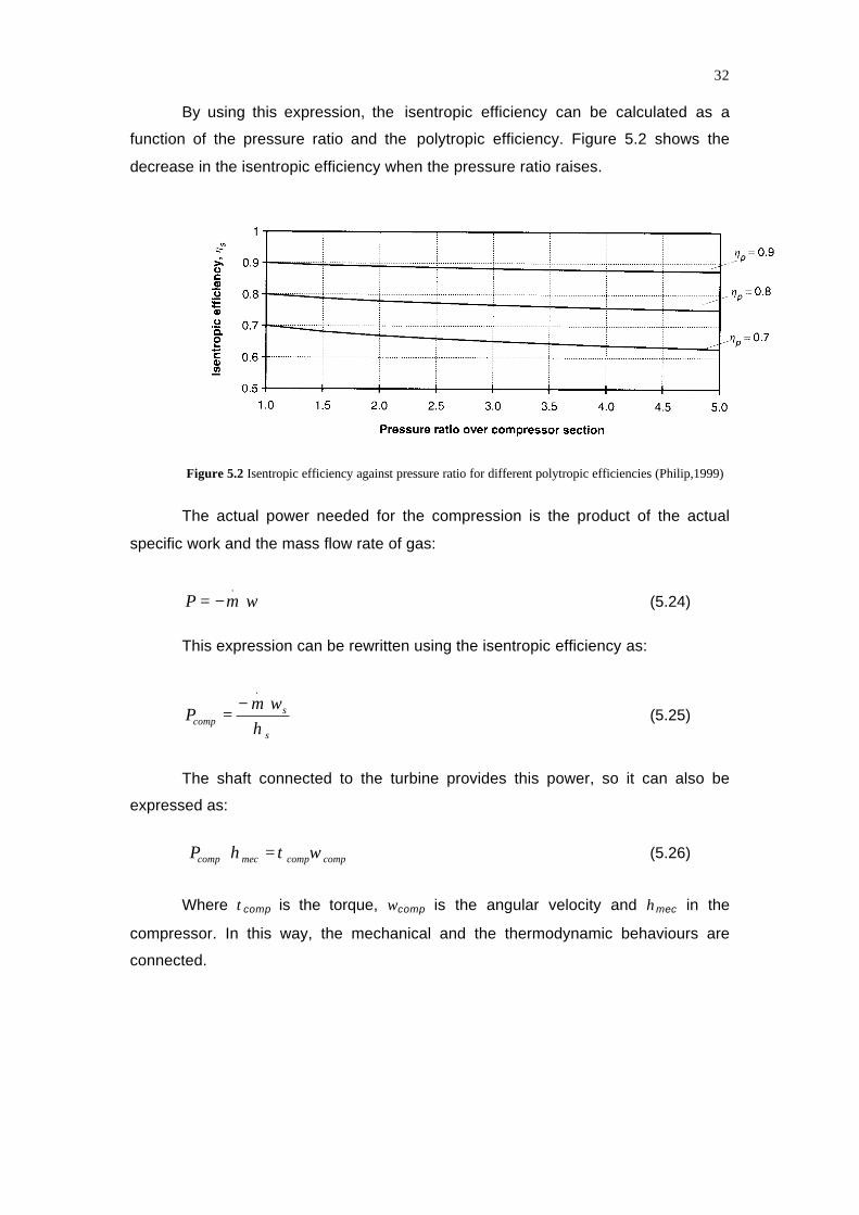
By using this expression, the isentropic efficiency can be calculated as a

function of the pressure ratio and the polytropic efficiency. Figure 5.2 shows the

decrease in the isentropic efficiency when the pressure ratio raises.

Figure 5.2 Isentropic efficiency against pressure ratio for different polytropic efficiencies (Philip,1999)

The actual power needed for the compression is the product of the actual

specific work and the mass flow rate of gas:

wmP ⋅−=.

(5.24)

This expression can be rewritten using the isentropic efficiency as:

s

scomp

wmP

η⋅−

=

.

(5.25)

The shaft connected to the turbine provides this power, so it can also be

expressed as:

compcompmeccompP ωτη =⋅ (5.26)

Where τcomp is the torque, ωcomp is the angular velocity and ηmec in the

compressor. In this way, the mechanical and the thermodynamic behaviours are

connected.

33

5.3 Use of the compressor map

The map of the manufacture was used for the implementation of the

compressor model. In this map, the pressure ratio is plotted against the corrected

mass flow for a range of corrected speed and polytropic efficiency curves. The

corrected mass flow and the corrected compressor speed are used in the map to

compensate for different environmental conditions under which the steady state

experiments were carried out.

For the compressor map, the corrected mass flow is defined as:

1

1

.

p

Tmmcor

⋅= (5.26)

And the corrected rotational speed:

1Tn

ncor = (5.27)

It is important to point out that there are two critical regions that have to be

taken into account, the surge and the stall lines. Along the surge line, the rotor speed

contours become nearly horizontal. To the left of the surge line, the speed contours

drop with respect to the pressure ratio. This may create an unstable phenomenon

called surging, which can destroy the compressor (Cohen, 1996). At each rotor

speed, a pressure for which surge occurs can be identified. Along the stall line, the

mass flow becomes choked. These regions have to be implemented in the model.

Figure 5.3 shows an example of compressor map. Surge line is indicated in

the figure.

All the information given in the map must to be processed by the model. It is

necessary to translate the information from the graphical form supplied by the

manufacturer to the Modelica model. There are several methodologies for

transforming this information.

34

Figure 5.3 Map for a centrifugal compressor (Cohen,1999)

One of these approaches could be to place all the information provided in

tables by choosing several points of the map and then to use these tables in a look-

up manner (Munns, 1996). But using the information, it can cause problems in the

dynamic simulations. In these tables, data points for several pressure ratios and

speed parameters are given. When a point for a different pressure ratio or speed

parameter needs to be evaluated, linear interpolation has to be used. When a

dynamic simulation moves over one of the given points, there is a discontinuous

derivative caused by the linear interpolation, which yields in problems for the dynamic

simulation. For this reason, the approach was rejected.

Another approach is to implement a couple of functions where pressure and

speed parameter are given as inputs and the efficiency and the mass flow parameter

are obtained as output for each one of the functions (Gustafsson, 1998).

In order to get a function for evaluating the corrected mass flow, an ellipsoid

equation is used:

cby

ax zz

=

+

(5.28)

35

Figure 5.4 Ellipsoid curves for different values of z

In figure 5.4, a set of the curves is shown. These curves have been obtained

using the ellipsoid equation for different values of the parameter z. The values of a, b

and c are all equal to one.

The lines on the left are for lower values of z. When the value of z increases,

the shape of the curves obtained is very similar to shape of the corrected speed

curves in the map.

Now, it is going to be shown how to calculate the mass flow by using the

ellipsoid equation. First, z and ncor (corrected rotational speed) are assumed to be

fixed. The variable ncor is calculated from the angular velocity, which is a dynamic

state, and can thus be regarded as known. The variable z is a function of ncor.

For the value of the constant a in the ellipsoid equation, the value of the

mass flow when the pressure ratio equals one is given. This value corresponds to the

mass flow when the compressor is stalled. For calculating the value of the constant b,

the ellipse equation is used. Therefore, once the constant a is known, x and y are

given as inputs and b is obtained as an output. The value of x corresponds to the

pressure ratio at the surge line, while y corresponds to the mass flow at the surge

line. In this way, the equation takes the value of the map.

36

Figure 5.5 Estimation of the value of b

Once values a, b and z are known and x (pressure ratio) is given as an input, y

(mass flow) can be obtained easily by using the equation (5.28).

In order to be able to use this equation over the whole range of speeds, it is

necessary to have a, b, and z as functions depending on the corrected speed:

( )( )( )cor

cor

cor

nfz

nfbnfa

=

==

For calculating a as a function of the speed, the points defined in the map for

the eight constant corrected speeds were used. For each one of these speeds, the

values of the corrected mass flow at the pressure ratio one are read. Then a relation

between the mass flow at pressure one and the corrected speed is calculated by

fitting a polynomial to the data points. Finally it is possible to calculate a as a function

of the corrected speed:

012

23

34

4 ananananaa corcorcorcor +⋅+⋅+⋅+⋅= (5.29)

where a0, a1, a2, a3 and a4 are the coefficients of the polynomial fitting. The

same approach is adopted to obtain a function of b depending on the corrected

speed:

37

012

23

34

4 bnbnbnbnbb corcorcorcor +⋅+⋅+⋅+⋅= (5.30)

where b0, b1, b2, b3 and b4 are the coefficients of the polynomial fitting. The

value of z is calculated as a linear function of the corrected speed. A value z1 for the

lowest speed and another z2 for the highest speed are chosen, and in between a

linear interpolation is used:

( )( )minmax

121 nn

zznzz cor −

−⋅+= (5.31)

Once a, b and z are known, it is possible to use the ellipsoid equation for the

whole map. The pressure ratio x is given as input and the mass flow y is obtained as

output.

Figure 5.6 Valid region for calculation with ellipsoidal equation

The surge line of the map needs to be considered. If the compressor reaches

the surge line, the corrected mass flow is not the one calculated with the ellipsoid

equation (Figure 5.6).

38

Because of this, the corrected mass flow for a given pressure ratio has to be

calculated and then it is necessary to check if the surge line has been reached. A

polynomial relation can be fitted between the mass flow and the pressure ratio at the

surge line by using the points obtained in the map. The approach is the same that

was taken for calculating a and b:

012

23

34

4 mrmrmrmrmmsurge +⋅+⋅+⋅+⋅= (5.32)

Where msurge is the mass flow at the surge line for a given value of the

pressure ratio r.

In order to know if the surge line has been reached, the mass flow for a

given speed and pressure ratio is calculated by using the ellipsoid equation. Then the

mass flow at the surge line is evaluated with equation (5.32). Once both mass flows

have been calculated, they are compared:

surgemm surgeellipse →≤

Another function for calculating the polytropic efficiency of the compressor

was also needed, but getting a function for it was much more difficult, since the

information provided by the map was not very accurate.

For this reason, it was decided to create a speed-dependent function for

evaluating the value of the maximum efficiency. Then a function for the degradation

of this efficiency was fitted.

So first of all, a polynomial relation can be fitted between the corrected speed

and the value of the maximum efficiency:

012

23

34

4max mnmnmnmnm corcorcorcor +⋅+⋅+⋅+⋅=η (5.33)

where m0, m1, m2, m3 and m4 are the constants for the polynomial fitting. The

same can be done between the speed and the pressure ratio for maximum efficiency:

012

23

34

4max_ pnpnpnpnpp corcorcorcoreff +⋅+⋅+⋅+⋅= (5.34)

where p0, p1, p2, p3 and p4 are the constants for the polynomial fitting. The

maximum polytropic efficiency and the corresponding pressure ratio for the present

corrected speed are calculated with equation (5.33) and (5.34). The actual pressure

39

ratio supplied may not be the optimum one, and the actual efficiency can be lower.

The difference in optimum pressure ratio can be expressed as a difference in

optimum flow. Once this difference is known, a correction for the efficiency is made.

This correction assumes a symmetrical degradation on both sides of the optimum

flow. This degradation is based on a parabolic equation:

( )2max_max effmmc −⋅−= ηη (5.35)

Where c is a constant. For fitting this constant several points on the map were

chosen.

40

5.4 Compressor model in Modelica

The compressor model belongs to the class of flow models. It uses the

equations explained at the beginning of this chapter in order to evaluate the mass

and energy flows. These flows provide the control volumes the information to

evaluate the mass and energy balances, as it was explained in chapter [4], which

was dedicated to the ThermoFlow library. An equation to link the thermal power to

the mechanical power is also needed.

A brief explanation of the implementation of the models is given here. All the

models used for the creation of the compressor are in a package called

NewCompressors.

CorrectedMass1

It is a function used to calculate the corrected mass flow by using

equation (5.28). Corrected speed and pressure ratio are the inputs of this

function.

CorrectedMass2

Corrected mass flow at the surge line is calculated here by using the

equation (5.32). Pressure ratio is needed as input.

P_maxeff

The value of pressure at the maximum efficiency for a given speed is

calculated here by using equation (5.34).

Maxeff

The value of maximum efficiency for a given speed is calculated here

by using equation (5.33).

Efficiency

The function with the degradation of the efficiency is given here

(equation (5.34.)). Corrected speed and pressure ratio are the inputs and the

polytropic efficiency is the output. Values obtained in P_maxeff and maxeff

are used internally in this function.

41

CompressorMap

This class uses the functions CorrectedMass1 and CorrectedMass2

for evaluating the actual mass flow in the compressor. A Boolean variable

called Surge is defined here. This variable is used to check if the compressor

reaches the surge line. The difference between the corrected mass flow in the

compressor and the corrected mass flow for the same pressure ratio at the

surge line is defined in a variable. Hence, it is possible to know how close is

the compressor to the surge line

IsentropicVariables

The class IsentropicVariables is a record. A record is a restricted form

of class that may not have any equations. It is used for setting different

variables not defined in the main model.

FlowModelBaseMD

The model called FlowModelBaseMD inherits the class

FlowVariablesMultiStatic, which was already available, in the ThermoFlow library.

This class is a shell model with two connectors for flow model. The connectors

contains the following variables:

§ mass fraction for each component of the mixture

§ pressure

§ enthalpy

§ mass flow for each component of the mixture

§ energy flow

§ density

§ Ratio of specific heat capacities

§ entropy

The class connects the variables internal to the model, to the variables at

the connector a and b.

42

PolytropicEfficiency

The class PolytropicEfficiency inheritances all the variables from the

class IsentropicVariables. Polytropic efficiency is calculated In this class by

using the functions P_maxeff, Maxeff and Efficiency. Once this is known, the

isentropic efficiency is used to evaluate the specific work in the compressor.

Compressor

The class Compressor is the complete thermodynamic model. It

inherits all the classes explained above.

Figure 5.7 Icon of the class Compressor

CompressorMec

In the model CompressorMec, equation (5.26), which links the

thermodynamical and mechanical behaviour, is added. A new connector for

the mechanical information is also added. This connector contains the

following variables:

§ Absolute rotation angle of flange

§ Torque in the flange

43

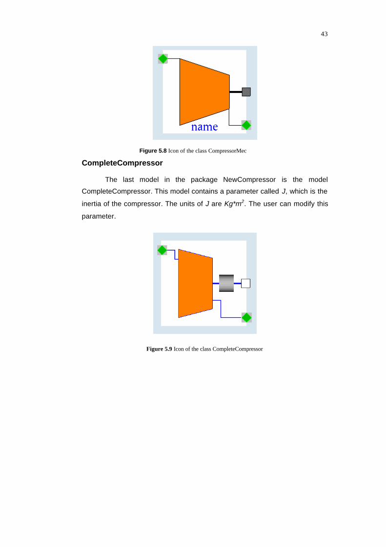
Figure 5.8 Icon of the class CompressorMec

CompleteCompressor

The last model in the package NewCompressor is the model

CompleteCompressor. This model contains a parameter called J, which is the

inertia of the compressor. The units of J are Kg*m2. The user can modify this

parameter.

Figure 5.9 Icon of the class CompleteCompressor

44

6.Turbine

6.1 Governing equations

One form of the energy equation for general steady state flow is given by the

following equation, (Cohen,1996):

0=−−−− gdzcdcdhdwdq (6.1)

where the dq is the specific external heating, dw is the specific work, dh is the

enthalpy, cdc is the kinetic energy term and gdz the potential energy term. The terms

dq and dz can be neglected, because the flow is adiabatic and the height change is

very small. Integrating between the 1 (inlet section of the turbine) and 2 (outlet

section of the turbine), the following expression is obtained:

021

21 2

22211 =−⋅+−⋅+ wchch (6.2)

Where w is the specific work obtained in the turbine and c and h are speed

and enthalpy. The kinetic energy term at the inlet of the turbine can be neglected,

because the air flow velocity at the turbine entrance is close to zero. For neglecting

the value of the kinetic term at the output of the turbine, the following consideration

can be taken. A value for the velocity in the output of 200 m/s has associated a

specific kinetic energy of 20 kJ/kg. The specific enthalpy of the air from tables, at the

temperature of 900°C is 1023.25 kJ/kg. It means that the kinetic term is 1.917 % of

the enthalpy of the air. It gives us an idea about the size of both terms. After this

consideration, it seems logical to neglect the kinetic terms for the dynamic model

(Philip,1999). Therefore, the next equation arises:

21 hhw −= (6.3)

A constant specific heat was also assumed for the turbine. A constant specific

heat cp for the model is calculated as an average for the temperatures at turbine inlet

and outlet. Therefore, equation (6.3) can be rewritten using the temperatures:

−⋅⋅=−⋅=

1

2121 1)(

TT

TcTTcw pp (6.4)

45

Using equation (5.6) of the chapter [5], it is possible to rewrite equation (6.4)

as:

−⋅⋅⋅

−=

1

21 1

1 TT

TRwγ

γ(6.5)

If the expansion process occurs in isentropic conditions, the work obtained is

the isentropic work:

−⋅⋅⋅

−=

1

21 1

1 TT

TRw ss γ

γ (6.6)

where T2s is the isentropic temperature. For an isentropic expansion, the

relation between pressures and temperatures is:

( )γ

γ 1

2

1

2

1

−

=

pp

TT

s

(6.7)

So expression (6.6) can be rewritten as:

−⋅⋅⋅

−=

−γ

γ

γγ

1

1

21 1

1 pp

TRw ss (6.8)

The isentropic efficiency for a turbine is defined as the ratio between the

actual enthalpy difference and the isentropic enthalpy difference:

12

12

hhhh

ss −

−=η (6.9)

Where h2s is the enthalpy at the outlet when the process is isentropic. As it

happens in the compressor, when pressure ratio changes, the isentropic efficiency

does not remain constant. For the case of the turbine, ηs tends to increase when the

pressure ratio grows, (Cohen, 1996). In order to take this into account, polytropic

efficiency is introduced:

turbine wholefor theconstant s

==dwdw

pη (6.10)

46

Following the same approach that was followed in chapter [5], it is possible to

get a function for evaluating the isentropic efficiency as a function of the polytropic

efficiency and the pressure ratio:

( )

( )

−⋅⋅

−⋅⋅

=−

−

γγ

η1

1

21

1

1

21

1

1

pp

Tc

pp

Tc

p

mm

p

s (6.11)

Where the coefficient m is:

( ) γγηγ

+−⋅=

1p

m (6.12)

Expression (6.9) and (6.11) can be combined in order to evaluate the actual

specific work in the turbine:

−⋅⋅⋅

−⋅=−

−γ

γ

γγ

η

1

1

21 1

1 pp

TRw s (6.13)

The actual power released in the expansion is the product of the actual

specific work and the mass flow rate of gas:

wmP ⋅=.

(6.14)

For taking into account the mechanical losses, the mechanical efficiency is

introduced:

mecml PPPP η⋅=−=' (6.15)

where P’ is the mechanical shaft power and Pml is the term referred to

mechanical losses. Then, mechanical and thermal power can be connected:

mecturtur PP ηωτ ⋅==' (6.17)

47

6.2 Turbine map

For the case of the compressor, the manufacturer provided a map for

evaluating the mass flow and the efficiency. For turbines there are also maps but

they have special characteristics. A typical map for a turbine can be seen in figure

6.1. The performance is expressed by plotting the polytropic efficiency ηp and the

corrected mass flow against the pressure ratio for various values of the corrected

speed.

For the turbine map, corrected flow mass is defined as:

1

1

.

p

Tmmcor

⋅= (6.26)

And the corrected speed of rotation:

1Tn

ncor = (6.27)

Where the subscript 1 is referred to the input of the turbine. The map shows

the relative speed to the design value:

Figure 6.1 Map of a turbine (Cohen, 1996)

48

The efficiency plot shows that the efficiency remains constant over a wide

range of corrected speeds and pressure ratios. For the case of the corrected mass

flow, the maximum value of it is reached at a pressure ratio, which produces choking

conditions at some point in the turbine. In this situation all the constant speed lines

merge into a single horizontal line as indicated on the mass flow plot.

Taking into account that for the dynamic simulation the turbine works in

choked conditions, a good approximation can be to assume that the corrected mass

flow remains constant. In this way, the equation for the design of nozzles is used for

evaluating the mass flow (Cohen,1996):

( )( )1

1

1

1

12 −

+

+

⋅=⋅

⋅ γγ

γγRpA

Tm

thr

(6.28)

Where Athr is the equivalent nozzle throat area. This equation is used for

dimensioning the nozzle area based on a known design point. Therefore, Athr can be

evaluated knowing the rest of variables at the design point. Then, this area is used to

evaluate the mass flow.

The efficiency is assumed constant for all the range of speeds. The user can

adjust the value of the efficiency.

49

6.3 Turbine model in Modelica

The turbine model implemented in Modelica is essentially a flow model. The

equations described in this chapter are included in the model. The model is very

similar to the compressor model, but the turbine model does not include a class for

the implementation of the map. In the turbine model this map is replaced by equation

(6.28), where choked conditions are assumed. The classes used for the creation of

the turbine model are located in the package NewTurbines. Some of the classes in

this package are described in the rest of the chapter.

FlowModelBaseDM

FlowModelBaseMD is a shell model with two connectors for flow

model. The connectors contains the following variables:

§ mass fraction for each component of the mixture

§ pressure

§ enthalpy

§ mass flow for each component of the mixture

§ energy flow

§ density

§ Ratio of specific heat capacities

§ entropy

The class connects the convent variables internal to the model, to the

variables at the connector a and b.

IsentropicVariables

The class IsentropicVariables is a record. In this record, different

variables, which are necessary for the turbine model, are defined.

PolytropicEfficiency

This class includes equations for calculating the isentropic efficiency

as a function of the polytropic efficiency and the pressure ratio. Isentropic

efficiency then is used to evaluate the specific work obtained in the turbine.

50

Turbine

The Turbine class is the complete thermodynamic model. All the

classes that were shown above are inherited from this class. Therefore, mass

and energy flows are evaluated in this model.

Figure 6.2 Icon of the class Turbine

TurbineMec

This class includes equation (6.17), which links the mechanical power

to the thermal power. A mechanical connector is included. The mechanical

connector contains the following variables:

§ Absolute rotation angle of flange

§ Torque in the flange

Figure 6.3 Icon of the class TurbineMec

51

CompleteTurbine

This model includes the model Inertia, which is inherited from the

Rotational library of Modelica. This model is a rotational component with

inertia and two rigidly connected flanges. The model includes the following

equation:

∑=⋅n

iiaJ τ (6.29)

where J is the moment of inertia, a is the angular acceleration, τ is the

torque and n is the number of mechanical connectors.

Figure 6.4 Interior of the class Complete Turbine

The moment of inertia is a parameter that can be supplied by the user.

Figure 6.5 Icon of the class CompleteTurbine

52

7.Combustion Chamber

7.1 Introduction

Models presented in previous chapters were limited to be non-reacting

thermodynamic systems. On the other hand, for the model of the combustion

chamber, chemical reactions must be taken into account. In non-reacting systems

just the notions of sensible internal energy (associated with temperature and

pressure changes) and latent internal energy (associated to phase changes) were

used. When dealing with reacting systems, it is necessary to consider the chemical

internal energy, which is associated with the destruction and the formation of

chemical bonds between the atoms.

In the combustion chamber, the chemical reaction involved is called

combustion. In a combustion, some molecules are destroyed for the creation of new

molecules with a release of a large amount of energy. Consequently, the energy and

mass balances have to include the chemical equation of the combustion. Normally,

energy and mass balances are treated in control volumes, but since chemical

reactions are involved a new class had to be developed.

Some additional assumptions have to be made for the derivation of the

model. These assumptions are:

§ The combustion is going to be considered as instantaneous. This is very a

logical consideration since the transients involved in the combustion are

much faster than all other transients in the system.

§ Kinetic and potential energy are going to be neglected in the energy

balance.

§ The efficiency of the combustion chamber is assumed as a constant

parameter, i.e. the user can select the desired value before running the

simulation.

53

7.2 Governing equations

Chemical equations govern the behaviour of the combustion chamber. In this

section, equations for energy and mass balances are shown. The assumption of

ideal gas properties for all components is used for calculating all the properties of the

gas mixtures.

Mass balance

The air is considered as a mixture of CO2, H2O, N2 and O2. The fuel used for

the turbine is natural gas. The composition of the natural gas is variable, depending

on the provider. Natural gas is mainly composed of a mixture of hydrocarbon fuels,

but other gases can also be found in it. For the model, natural gas is considered as a

mixture of the following elements: CH4, C2H6, C3H8, C4H10, N2 and CO2. From the

chemical point of view, N2, CO2, which can be found either in the air or in the fuel,

and H2O, which can be found just in the air, are assumed to be inert. It means that

they are not involved in any chemical reaction. Therefore, only hydrocarbon fuels

(CH4, C2H6, C3H8 and C4H10) react. The chemical equation for the combustion of a

general hydrocarbon fuel assuming the stoichiometric amount of O2 is:

OHn

COmOn

mHC nm 222 24⋅

+⋅→⋅

++ (7.1)

Where m and n depend on the kind of hydrocarbon, e.g for Methane m and n

are equal to 1 and 4. Equation (7.1) implies that each kmol of CmHn reacts with

(m+n/4) kmol of O2, producing m kmol of CO2 and (n/2) kmol of H2O. According to

this, the following expressions arise for CH4, C2H6, C3H8 and C4H10:

OHCOOCH 2224 22 ⋅+→⋅+ (7.2)

OHCOOHC 22262 325.3 ⋅+⋅→⋅+ (7.3)

OHCOOHC 22283 435 ⋅+⋅→⋅+ (7.4)

OHCOOHC 222104 545.6 ⋅+⋅→⋅+ (7.5)

Complete combustion is assumed, which means that there is not CO among

the products and all hydrocarbon fuel is consumed in the reaction.

54

It is possible to transform expressions (7.2), (7.3), (7.4) and (7.5) into

expressions for mass flow (kg/s) by using the molecular weight of the components

involved in the reactions:

component of kmolcomponent of kg

weightmolecular =→ w (7.6)

In this way:

OHwCH

OwHCO

wCHwCO

OwCHwO

CH 24

22

4

22

4

24 22 ⋅

⋅+⋅

→⋅

⋅+

(7.7)

OHHwCOwH

COHwC

wCOO

HwCwO

HC 262

22

62

22

62

262 325.3 ⋅

⋅+⋅

⋅→⋅

⋅+

(7.8)

OHHwCOwH

COHwC

wCOO

HwCwO

HC 283

22

83

22

83

283 435 ⋅

⋅+⋅

⋅→⋅

⋅+

(7.9)

OHHwCOwH

COHwC

wCOO

HwCwO

HC 2104

22

104

22

104

2104 545.6 ⋅

⋅+⋅

⋅→⋅

⋅+

(7.10)

Where wCO2, wCH4, wC2H6, wC3H8, wC4H10, wH2O and wO2 are the molecular

weighs of CO2, CH4, C2H6, C3H8, C4H10, H2O and O2 respectively.

Equations above used the soichiometric amount of O2. If the amount of O2 is

bigger than the stoichiometric, there is O2 in the exhausted gases. Gas turbines

operate with excess of air, i.e. O2 is not totally consumed in the reaction. Therefore,

the composition of the exhausted gases for the gas turbine is a mixture of CO2, H2O,

N2 and O2. Mass flows for each one of the components at the outlet of the

compressor can be evaluated by using the expressions (7.7), (7.8), (7.9) and (7.10).

Considering that min [CO2], min [H2O], min [N2] and min [O2], are the mass flows of

CO2, H2O, N2 and O2.at the inlet of the combustion chamber, and mfuel [CH4], mfuel

[C2H6], mfuel [C3H8], mfuel [C4H10], mfuel [N2], mfuel [CO2] are the mass flows of CH4, C2H6,

C3H8, C4H10, N2 and CO2, the following relation can be written:

55

[ ] [ ] [ ]

[ ] [ ]

[ ] [ ]2104

2104

83

283

62

262

4

2422

4

32

COmHwC

wCOHCm

HwCwCO

HCmHwC

wCOHCm

wCHwCO

CHmCOmCOm

fuelfuel

fuelfuel

fuelinout

+⋅⋅+

+⋅⋅+⋅⋅+

+⋅+=

(7.11)

[ ] [ ] [ ]

[ ] [ ]

[ ]104

2104

83

283

62

262

4

2422

5

43

2

HwCOwH

HCm

HwCOwH

HCmHwCOwH

HCm

wCHOwH

CHmOHmOHm

fuel

fuelfuel

fuelinout

⋅⋅+

+⋅⋅+⋅⋅+

+⋅⋅+=

(7.12)

[ ] [ ] [ ]222 NmNmNm fuelinout += (7.13)

[ ] [ ] [ ]

[ ] [ ]

[ ]104

2104

83

283

62

262

4

2422

5.6

55.3

2

HwCOwH

HCm

HwCwO

HCmHwC

wOHCm

wCHwO

CHmOmOm

fuel

fuelfuel

fuelinout

⋅⋅−

−⋅⋅−⋅⋅−

−⋅⋅−=

(7.14)

Where mout [CO2], mout [H2O], mout [N2] and mout [O2], are the mass flows of

CO2, H2O, N2 and O2.at the outlet of the combustion chamber.

Energy Balance

Once the mass balance is calculated, the next step is to evaluate the energy

balance. Now it is necessary to use the concept of enthalpy of formation.

It is possible to establish a reference for enthalpy in the study of reactive

systems by setting the value zero to the enthalpy of the stable elements in a state

called standard reference state defined for Tref=298.15 K and pref=1 atm. Stable

elements are set to zero at the standard conditions. The term stable is used in the

meaning chemically stable. This means that at the standard state, the stable forms of

Nitrogen, Oxygen and Hydrogen are N2, O2 and H2 and not N, O and H. Using this

reference, it is possible to assign values for the enthalpy of formation of the

components. The enthalpy of formation of a component at the standard reference

state, is the value of the energy that is released or absorbed for the same when it is

56

created from its primary forms (O2, C, H2,...), at Tref and pref. If the enthalpy of

formation is negative, energy is released during the creation of the component, and

when it is positive, energy is absorbed during the process. If the conditions differ from

the standard reference, the enthalpy of formation will decrease or increase. For

example, if the temperature of the components is higher than Tref, the released

energy decreases because some energy is needed to raise the temperature.

Consequently, before writing the energy balance, it is necessary to express

the enthalpy of a component in a form suitable for use in reacting systems. The

enthalpies of formation of each of the components need to be taken into account for

the energy balance in the combustion chamber. A new definition of enthalpy called

total enthalpy is introduced. This enthalpy is the sum of the enthalpy of formation of

the component at 25 C and 1 atm and the sensible enthalpy of the component of the

component relative to the reference temperature:

( )Ref0 hhhEnthalpy f −+= (7.15)

In ThermoFlow, zero Kelvin is chosen as the reference state for calculating

the enthalpy. The expression implemented in ThemoFlow for calculating the sensible

enthalpy is based on the NASA tables (Gordon,1994).

With the enthalpy defined as above, including the enthalpy of formation, the

energy balance can be evaluated. When the changes in kinetic and potential

energies are negligible, the conservation of energy relation for a chemically reacting

steady-flow system can be expressed in the following form (Cengel, 1994):

( )( ) ( )( )rfrpfp

hhhmhhhmWQ ref0

.

ref0

...

−+⋅−−+⋅=− ∑∑ (7.16)

Where the subscript p is taken to refer products, while r refers to reactants. In

the combustion chamber, the work term can be neglected. Then, the chemical

energy released during a combustion process is either lost as heat to the

surroundings or it is used internally to raise the temperature of the combustion

products. In the limit case of no heat loss to the surroundings (Q=0), the temperature

of the products will reach a maximum, which is called the adiabatic flame or adiabatic

combustion temperature. In this case, the expression (16) can be rewritten as:

57

( )( ) ( )( )rfrpfp

hhhmhhhm ref0

.

ref0

.

−+⋅=−+⋅ ∑∑ (7.17)

In gas turbines, the highest temperature to which the blades can be exposed

is limited by metallurgical considerations. Therefore, the adiabatic temperature is an

important factor in the design of gas turbines. The maximum temperatures which

occurs in gas turbines are considerably lower than the adiabatic flame temperature

due to the following reasons:

§ When a combustion chamber operates with excess of air, which is the

normal case, it serves as a coolant

§ The combustion is usually incomplete

§ Some heat loss takes place

§ Some combustion gases dissociate at high temperatures

For taking into account the first three points, the combustion efficiency (ηcc)

can be introduced, so expression (7.17) is rewritten as:

( )( ) ( )( )

−+⋅⋅=−+⋅ ∑∑ rfrccpfp

hhhmhhhm ref0

.

ref0

.

η (7.18)

58

7.3 Combustion chamber model in Modelica

In the chapter [4], it was explained that the construction of model was based

in an alternative sequence of flow models and control volumes. The mass and

energy balances are calculated in the control volumes. But for the model of the

combustion chamber, mass and energy balances are implemented in a flow model.

For the case of the combustion chamber, equations explained above are used to

evaluate the mass and energy balances. An equation for calculating the relation

between the mass flow and the variation of the pressure is also needed. The

combustion chamber model evaluates the mass and energy flows, which are then

used in the control volume for evaluating the mass and energy balances.

Temperature in the combustion chamber is obtained there.

All the models used for the creation of the combustion chamber are in the

package called CombustionChamber.

Some of the classes included in this package are explained briefly.

MassBalance.

This class is used for evaluating the composition of each of the

components of the gas mixture at the output of the combustion chamber. This

class contains the equations (7.11), (7.12), (7.13) and (7.14)

Valve

This model was created for controlling the mass flow of fuel into the

combustion chamber. The model Valve is a simple flow model, with two flow

connectors and one connector with an input signal. This last connector is

used to regulate the fuel flow. There is a parameter called mdot_max, which

can be supplied by the user. This parameter is the maximum fuel flow in kg/s

that the valve can supply. It is possible to regulate this fuel flow by using an

input signal with a value between zero and one.

NaturalGasResS_pTX

The model simulates an infinitive reservoir of natural gas. It is a

control volume in which pressure p and temperature T can be assigned. The

model also includes a medium model for natural gas, which includes the

components CH4, C2H6, C3H8, C4H10, N2 and CO2. The user can select the

natural gas fuel composition in fuel in % of mass fraction.

59

ThreePort

This class is essentially a three port flow model. These three

connectors are used for the incoming air, fuel and exhausted gases,

respectively. This class also inherits the record called

FlowVariablesSingleStatic, which contains some necessary variables for a

flow model. In this class, these variables are connected to the variables in the

connectors.

CombustionChamber

This model is the real combustion model. It inherits the classes

ThreePort and MassBalance. The model contains an equation that relates the

mass flow m to the pressure drop in the combustion chamber. The equation

is the following:

0

20

..2

dpm

dpm

= (7.19)

Where dp is:

21 ppdp −= (7.20)

and m0 and dp0 are the mass flow m and pressure loss dp in the

combustion chamber at the design point.

The energy balance of equation (7.18) is also included in this class.

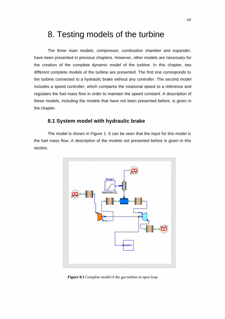
60

8. Testing models of the turbine

The three main models, compressor, combustion chamber and expander,

have been presented in previous chapters. However, other models are necessary for

the creation of the complete dynamic model of the turbine. In this chapter, two

different complete models of the turbine are presented. The first one corresponds to

the turbine connected to a hydraulic brake without any controller. The second model

includes a speed controller, which compares the rotational speed to a reference and

regulates the fuel mass flow in order to maintain the speed constant. A description of

these models, including the models that have not been presented before, is given in

the chapter.

8.1 System model with hydraulic brake

The model is shown in Figure 1. It can be seen that the input for this model is

the fuel mass flow. A description of the models not presented before is given in this

section.

Figure 8.1 Complete model of the gas turbine in open loop

61

In order to define environmental conditions e.g. temperature, pressure,

composition of the air, it was necessary to develop a model of the environment. In

the ThermoFlow library, thermodynamic reservoirs are used for this purpose. A

reservoir is considered as a control volume of infinite size, i.e. the values of the

states do not change when energy and mass are introduced or extracted. In the

turbine model, these states are temperature, pressure and composition of the mixture

of the gases CO2, H2O, N2 and O2. These states are parameters, which can be

modified by the user for each simulation. In this way, it is easy to choose different

environmental conditions for the simulations. However, the compressor and the

turbine are not connected directly to the environment. Pipes and filters cause a

pressure drop between the atmospheric pressure and the pressures at the inlet of the

compressor and at the outlet of the combustion chamber. In order to take this into

account, a flow model with a simple equation for the pressure drop is added to the

reservoir model. The complete model created by a reservoir and a pressure drop

model is called source. Two air sources are used in the turbine model, one situated

at the beginning of the cycle, i.e. before the compressor and another at the end of the

cycle, i.e. after the expander.

Another reservoir is used for simulating the fuel tank. Nevertheless, the states

for this reservoir are pressure, temperature, and composition of the mixture of the

gases CH4, C2H6, C3H8, C4H10, N2 and CO2. In this way, it is possible to set different

compositions of natural gas for the experiments.

In order to extract the power obtained in the expander without having to

control the process, a model of a brake is needed to dissipate the energy. A hydraulic

brake model was implemented for the turbine system model. This model is based on

a relation between the torque and the speed. The relation is parabolic:

221 ncc ⋅+=τ

Where τ is the torque, n is the rotational speed and c1 and c2 are

parameters, which can be modified by the user. In this way, the model can be

simulated for different speeds by varying the values of c1 and c2.

The model also contains four control volumes. As it was explained in the

ThermoFlow chapter, control volumes are used for evaluating the mass and energy

balances. The area and length of the control volumes are parameters and have to be

set by the user.

62

8.2 System model with speed controller

This second model can be used for reproducing situations which are closer to

the actual use of the turbine in the pilot plant. This model is very similar to the model

explained above, but the model of the brake is replaced by providing a torque as an

input, which could e.g. come from a generator. When the value of the torque

increases, the speed decreases. The value of the speed is compared to the

reference speed and the controller increases the value of the fuel mass flows, in

order to increase the speed until it reaches steady state. The model of the PI

controller was taken from the Block sub-library. The complete model can be seen in

the figure.

Figure 8.2 Complete model of the gas turbine with a speed controller

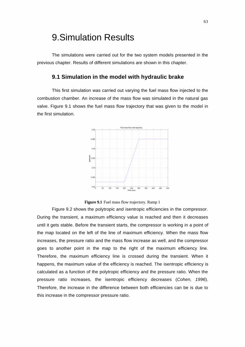
63

9.Simulation Results

The simulations were carried out for the two system models presented in the

previous chapter. Results of different simulations are shown in this chapter.

9.1 Simulation in the model with hydraulic brake

This first simulation was carried out varying the fuel mass flow injected to the

combustion chamber. An increase of the mass flow was simulated in the natural gas

valve. Figure 9.1 shows the fuel mass flow trajectory that was given to the model in

the first simulation.

Figure 9.1 Fuel mass flow trajectory. Ramp 1

Figure 9.2 shows the polytropic and isentropic efficiencies in the compressor.

During the transient, a maximum efficiency value is reached and then it decreases

until it gets stable. Before the transient starts, the compressor is working in a point of

the map located on the left of the line of maximum efficiency. When the mass flow

increases, the pressure ratio and the mass flow increase as well, and the compressor

goes to another point in the map to the right of the maximum efficiency line.

Therefore, the maximum efficiency line is crossed during the transient. When it

happens, the maximum value of the efficiency is reached. The isentropic efficiency is

calculated as a function of the polytropic efficiency and the pressure ratio. When the

pressure ratio increases, the isentropic efficiency decreases (Cohen, 1996).

Therefore, the increase in the difference between both efficiencies can be is due to

this increase in the compressor pressure ratio.

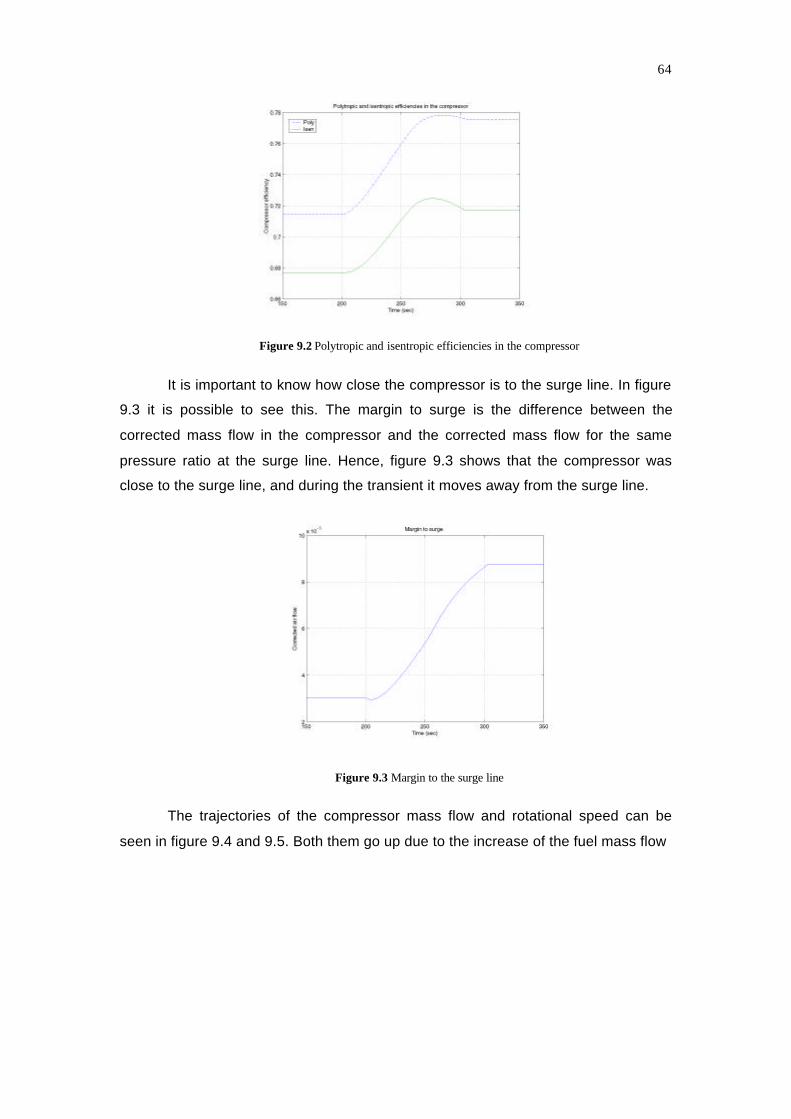
64

Figure 9.2 Polytropic and isentropic efficiencies in the compressor

It is important to know how close the compressor is to the surge line. In figure

9.3 it is possible to see this. The margin to surge is the difference between the

corrected mass flow in the compressor and the corrected mass flow for the same

pressure ratio at the surge line. Hence, figure 9.3 shows that the compressor was

close to the surge line, and during the transient it moves away from the surge line.

Figure 9.3 Margin to the surge line

The trajectories of the compressor mass flow and rotational speed can be

seen in figure 9.4 and 9.5. Both them go up due to the increase of the fuel mass flow

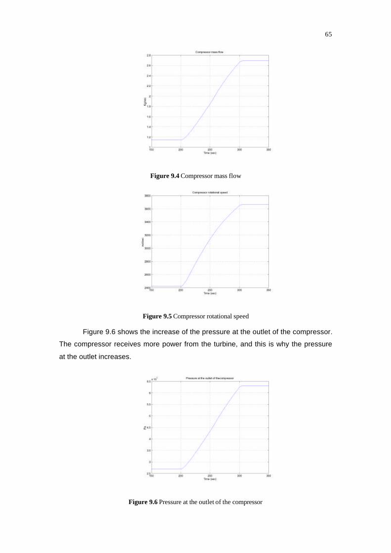
65

Figure 9.4 Compressor mass flow

Figure 9.5 Compressor rotational speed

Figure 9.6 shows the increase of the pressure at the outlet of the compressor.

The compressor receives more power from the turbine, and this is why the pressure

at the outlet increases.

Figure 9.6 Pressure at the outlet of the compressor

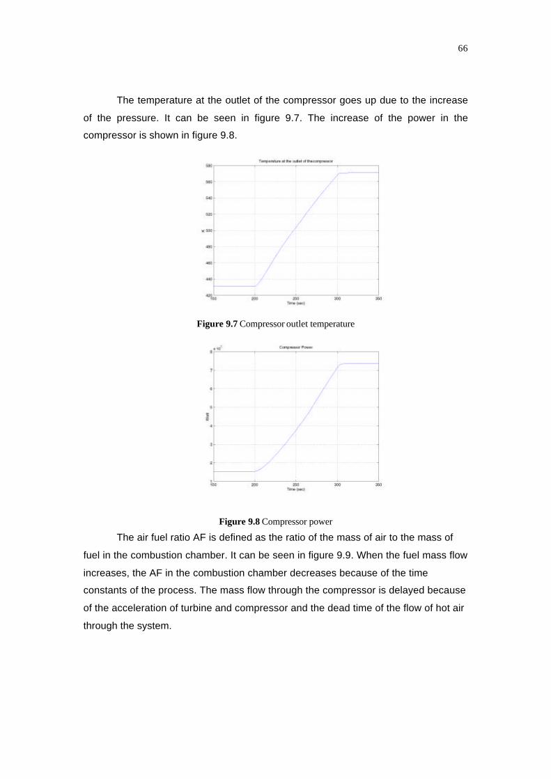
66

The temperature at the outlet of the compressor goes up due to the increase

of the pressure. It can be seen in figure 9.7. The increase of the power in the

compressor is shown in figure 9.8.

Figure 9.7 Compressor outlet temperature

Figure 9.8 Compressor power

The air fuel ratio AF is defined as the ratio of the mass of air to the mass of

fuel in the combustion chamber. It can be seen in figure 9.9. When the fuel mass flow

increases, the AF in the combustion chamber decreases because of the time

constants of the process. The mass flow through the compressor is delayed because

of the acceleration of turbine and compressor and the dead time of the flow of hot air

through the system.

67

Figure 9.9 Air-fuel ratio AF

The temperature in the combustion chamber is shown in Figure 9.10. This

temperature depends on the shape of the factor AF.

Figure 9.10 Combustion chamber temperature

Figures 9.11, 9.12, 9.13 and 9.14 show the mass flows of CO2, H2O, N2 and

O2 at the inlet and at the outlet of the combustion chamber.

68

Figure 9.11 CO2 mass flow

Figure 9.12 H2O mass flow

The mass flows of CO2 and H2O increase at the outlet due to the combustion.

Since the N2 was assumed to be inert, the mass flow is the same at the inlet and at

the outlet. However, the mass flow of O2 decreases because it is consumed in the

reaction.

69

Figure 9.13 N2 mass flow

Figure 9.14 O2 mass flow

It should be noted that at the beginning of the transient, the mass flow of O2

decreases. When the transient starts, the fuel mass flow increases and more O2 is

needed for reacting with the fuel. After a while, the amount of air flowing through the

compressor increases so the O2 at the outlet of the combustion chamber increases

as well.

Figure 9.15 shows the temperatures at the inlet and the outlet of the turbine.

The difference between both temperatures increases due to the increase in the

pressure ratio and the increase of the efficiency in the turbine.

70

Figure 9.15 Temperature at the inlet and aoutlet of the turbine

Figure 9.16 Isentropic efficiency in the turbine

Figure 9.16 shows the increase of the isentropic efficiency due to the increase

of the pressure ratio (Cohen,1996). Polytropic efficiency was assumed constant in

the turbine.

The power of the turbine is shown in Figure 9.17. Comparing to the power of

the compressor, it yields that around the 68% of the power goes to the compressor,

and the rest goes to the brake.

71

Figure 9.17 Turbine power

A different trajectory for the fuel gas was introduced to the system model in a

different simulation. The values of the fuel mass flow at the beginning and at the end

of the ramp were the same than in the first ramp but this ramp was faster than the

previous. The duration of the ramp was 10 sec, so ten times shorter than the first

one. The ramp can be observed in Figure 9.18.

Figure 9.18 Fuel mass flow trajectory. Ramp2

Temperatures at the combustion chamber for ramp 1 and ramp 2 are

compared in Figure 9.19. It is possible to see a higher increase in the temperature

obtained with the faster ramp (ramp 2). After a while, both temperatures reach the

same value. Therefore, the same increase in the fuel mass flow can yield different

transient temperatures in the turbine. This can not be reproduced by using a static

model.

72

Figure 9.19 Comparation of temperature for Ramp 1 and ramp 2

9.2 Simulation of the Model with speed controller

A power ramp was simulated for the model with the speed controller, by using

a torque as an input. Some results were compared to measurements carried out in

the real plant in 1997. The results of these experiments can be found in (Lindquist,

1999). Figure 9.20 shows the torque introduced to the model. It goes from zero, idle

conditions, to the maximum torque, 119 Nm. Assuming that the rotational speed is

constant and with a value of 4020 rpm, the maximum torque corresponds to a power

output of 480 KW.

Figure 9.20 Torque absorved by the brake

The air mass flow in the compressor is shown in Figure 9.21. In the

simulation, the value of the mass flow is 3.436 kg/s at idle and 3.33 kg/s at 480 KW.

The actual results in experiments gave a result of 3.45 kg/s at idle and 3.41 kg/s at

480, so the maximum error is 2.3%.

73

Figure 9.21 Compressor mass flow

Figure 9.22 shows the pressure at the outlet of the compressor. The results in

the simulation are 7.35 Bar and 8.3 bar at idle and at 480 KW respectively. The

actual results obtained in the experiments are 7.3 bar and 8.2 bar. The maximum

error is 1.2%.

Figure 9.22 Pressure at the outlet of the compressor

Figures 9.23 shows the temperature at the outlet of the compressor. The

actual temperature is around 600 K over the whole power output range. In the

simulation, the value of the temperature varies slightly from 616 K at idle to 626 at

480 KW. The maximum error comparing to actual data is 4.3%.

74

Figure 9.23 Temperature at the outlet of the compressor

The expander outlet temperature is shown in Figure 9.24. The results in the

simulation are 626 K and 828 K at idle and at 480 KW respectively. The actual result

goes from 623.5 K to 773 k. The maximum error is reached at 480 KW, and its value

is 7.3%.

Figure 9.24 Temperature at the outlet of the turbine

75

10. Conclusions and future work

10.1 Conclusions

Some of the conclusions obtained at the end of the work are:

§ The system turbine model reproduces well the dynamic behaviour of a

real plant. The results obtained when the model reaches stationary

conditions are very close to the results obtained in the experiments

carried out in the real plant. On the other hand, there was no data for

comparing to some results obtained simulating transients. However,

the results were discussed with people of the Heat and Power

Department, concluding that they results were close to reality

§ The model can be reused for different plants by changing some of the

classes. The model developed is general, with the exception of the

compressor map and the equation for the expander.

§ Some of the models can be used as new components of the

ThermoFlow library, continuing in this way the development of it.

10.2 Future work

The model developed and the results obtained were very interesting, but

improvements and extensions should be done. Better maps for compressor and

turbines can replace the present ones in order to simulate different transients, e.g. a

start-up of the plant. Models for the regenerative heat exchanger and evaporative

tower can be developed and added to the model in order to simulate the complete

plant.

76

Bibliography§ Philip, Thomas “Simulation of Industrial processes for Control Engineers”.

Butterworth-Heinemann (1999).

§ Cohen,H. ; Rogers GFC. ; Saravanamuttoo, HIH. Gas Turbine Theory”. Longman

Group Limited (1996).

§ Cengel, Y. A.; Boles, M.A.; “Thermodynamics, an engineering aproach”.

McGraw-Hill (1994).

§ Lindquist, T.; “Theoretial and Experimental Evaluation of the EvGT-Process”.

Licentiate Thesis. , Lund University ISRN LUTMDN/TMVK-99/7037--SE (1999).

§ Gustafsson.J.O “Static and Dynamic Modelling of Gas Turbine in Advanced

Cycles”. Licenciate Thesis. , Lund University ISRN LUTMDN/TMVK-98/7030--

SE(1998).

§ Modelica design group “Modelica- A Unified Object-Oriented Language for

Physical System Modeling. Tutorial and Rationale”. www.modelica.org (1999).

§ Eborn, J. ; Tummescheit, H. ; Wagner F.. “Thermoflow. A Thermo-Hydraulic

Library in Modelica. Documentation”. (2000).

§ Munns S.A. “Computer Simulation of Powertrain Components with Methodologies

for generalized system modeling”. Master of Sience. University of Wisconsin-

Madison (1996).

§ Eborn, J. “On Model Libraries for Thermo-Hydraulic Aplications”. Doctoral Thesis,

Lund University. ISRN LUTFD2/TFRT-1061-SE.(2001).