Embed Size (px)
Citation preview
ModelicaTM is a trademark of the "Modelica Design Group".
ModelicaTM - A Unified Object-OrientedLanguage for Physical Systems Modeling
LANGUAGE SPECIFICATION
Version 1.2 June 15, 1999
Modelica Language Specification
Modelica 1.2 2
Contents
1 Introduction ............................................................................................................................................... 5
1.1 Overview of Modelica ......................................................................................................................... 5
1.2 Scope of the specification .................................................................................................................... 5
1.3 Definitions and glossary ...................................................................................................................... 5
2 Modelica syntax ........................................................................................................................................ 7
2.1 Lexical conventions ............................................................................................................................. 7
2.2 Grammar.............................................................................................................................................. 7
2.2.1 Model definition............................................................................................................................. 7
2.2.2 Class definition .............................................................................................................................. 7
2.2.3 Extends........................................................................................................................................... 8
2.2.4 Component clause .......................................................................................................................... 8
2.2.5 Modification................................................................................................................................... 8
2.2.6 Equations........................................................................................................................................ 9
2.2.7 Expressions .................................................................................................................................. 10
3 Modelica semantics ................................................................................................................................. 13
3.1 Fundamentals..................................................................................................................................... 13
3.1.1 Scoping and name lookup ............................................................................................................ 13
3.1.1.1 Parents .................................................................................................................................... 13
3.1.1.2 Static name lookup ................................................................................................................. 13
3.1.1.3 Dynamic name lookup............................................................................................................ 14
3.1.2 Environment and modification..................................................................................................... 15
3.1.2.1 Environment ........................................................................................................................... 15
3.1.2.2 Merging of modifications ....................................................................................................... 15
3.1.2.3 Single modification ................................................................................................................ 17
3.1.2.4 Instantiation order................................................................................................................... 17
3.1.3 Subtyping and type equivalence................................................................................................... 17
3.1.3.1 Subtyping of classes ............................................................................................................... 17
3.1.3.2 Subtyping of components ....................................................................................................... 17
3.1.3.3 Type equivalence.................................................................................................................... 17
3.1.3.4 Type identity........................................................................................................................... 18
3.1.4 Classes on external files ............................................................................................................... 18
3.2 Declarations ....................................................................................................................................... 18
3.2.1 Component clause ........................................................................................................................ 18
3.2.2 Variability prefix.......................................................................................................................... 19
Modelica Language Specification
Modelica 1.2 3
3.2.3 Expressions .................................................................................................................................. 20
3.2.4 Vectors, Matrices, and Arrays...................................................................................................... 21
3.2.4.1 Array declarations .................................................................................................................. 21
3.2.4.2 Built-in Functions for Array Expressions............................................................................... 22
3.2.4.3 Vector, Matrix and Array Constructors .................................................................................. 24
Array Construction ........................................................................................................... 24
Array Concatenation ......................................................................................................... 24
Array Concatenation along First and Second Dimensions................................................ 25
Vector Construction.......................................................................................................... 26
3.2.4.4 Array access operator ............................................................................................................. 26
3.2.4.5 Scalar, vector, matrix, and array operator functions............................................................... 27
Numeric Type Class.......................................................................................................... 27
Equality and Assignment of type classes .......................................................................... 27
Addition and Subtraction of numeric type classes ............................................................ 27
Scalar Multiplication of numeric type classes .................................................................. 27
Matrix Multiplication of numeric type classes.................................................................. 28
Scalar Division of numeric type classes............................................................................ 28
Exponentation of Scalars of numeric type classes ............................................................ 28
Scalar Exponentation of Square Matrices of numeric type classes................................... 28
Slice operation .................................................................................................................. 28
Relational operators .......................................................................................................... 29
Functions........................................................................................................................... 29
Empty Arrays.................................................................................................................... 30
3.2.5 Final element modification .......................................................................................................... 30
3.2.6 Short class definition.................................................................................................................... 31
3.2.7 Local class definition ................................................................................................................... 32
3.2.8 Extends clause.............................................................................................................................. 32
3.2.9 Redeclaration ............................................................................................................................... 33
3.3 Equations ........................................................................................................................................... 34
3.3.1 Equation clause ............................................................................................................................ 34
3.3.2 If clause........................................................................................................................................ 34
3.3.3 For clause ..................................................................................................................................... 34
3.3.4 When clause ................................................................................................................................. 34
3.3.5 Assert ........................................................................................................................................... 35
3.3.6 Connections.................................................................................................................................. 35
3.3.6.1 Generation of connection equations ....................................................................................... 36
3.3.6.2 Restrictions............................................................................................................................. 36
Modelica Language Specification
Modelica 1.2 4
3.4 Functions ........................................................................................................................................... 36
3.5 Code Optimizations ........................................................................................................................... 38
3.6 Events and Synchronization............................................................................................................... 38
3.7 Restricted classes ............................................................................................................................... 40
3.8 Variable attributes.............................................................................................................................. 41
3.9 Intrinsic library functionality ............................................................................................................. 42
3.9.1 Built-in variable time ................................................................................................................... 42
3.9.2 Modelica built-in operators .......................................................................................................... 42
4 Mathematical description of Hybrid DAEs ............................................................................................. 47
5 Unit expressions ...................................................................................................................................... 50
5.1 The Syntax of unit expressions .......................................................................................................... 50
5.2 Examples ........................................................................................................................................... 51
6 External function interface ...................................................................................................................... 52
6.1 Overview ........................................................................................................................................... 52
6.2 Argument type mapping .................................................................................................................... 52
6.2.1 Simple types................................................................................................................................. 53
6.2.2 Arrays........................................................................................................................................... 53
6.2.3 Records ........................................................................................................................................ 55
6.3 Return type mapping.......................................................................................................................... 56
6.4 Aliasing.............................................................................................................................................. 56
6.5 Examples ........................................................................................................................................... 57
6.5.1 Input parameters, function value.................................................................................................. 57
6.5.2 Arbitrary placement of output parameters, no external function value ........................................ 57
6.5.3 External function with both function value and output variable .................................................. 58
7 Modelica standard library........................................................................................................................ 59
Modelica Language Specification
Modelica 1.2 5
1 Introduction
1.1 Overview of Modelica
Modelica is a language for modeling of physical systems, designed to support effective library development andmodel exchange. It is a modern language built on non-causal modeling with mathematical equations and object-oriented constructs to facilitate reuse of modeling knowledge.
1.2 Scope of the specification
The Modelica language is specified by means of a set of rules for translating a model described in Modelica tothe corresponding model described as a flat hybrid DAE. The key issues of the translation (or instantiation inobject-oriented terminology) are:
• Expansion of inherited base classes
• Parameterization of base classes, local classes and components
• Generation of connection equations from connect statements
The flat hybrid DAE form consists of:
• Declarations of variables with the appropriate basic types, prefixes and attributes, such as "parameterReal v=5".
• Equations from equation sections.
• Function invocations where an invocation is treated as a set of equations which are functions of all inputand of all result variables (number of equations = number of basic result variables).
• Algorithm sections where every section is treated as a set of equations which are functions of thevariables occuring in the algorithm section (number of equations = number of different assignedvariables).
• When clauses where every when clause is treated as a set of conditionally evaluated equations, alsocalled instantaneous equations, which are functions of the variables occuring in the clause (number ofequations = number of different assigned variables).
Therefore, a flat hybrid DAE is seen as a set of equations where some of the equations are only conditionallyevaluated (e.g. instantaneous equations are only evaluated when the corresponding when-condition becomestrue).
The Modelica specification does not define the result of simulating a model or what constitutes a mathematicallywell-defined model.
1.3 Definitions and glossary
The semantic specification should be read together with the Modelica grammar. Non-normative text, i.e.,examples and comments, are enclosed in [ ], comments are set in italics.
Term Definition
Component An element defined by the production component-clause in the Modelica
Modelica Language Specification
Modelica 1.2 6
grammar.
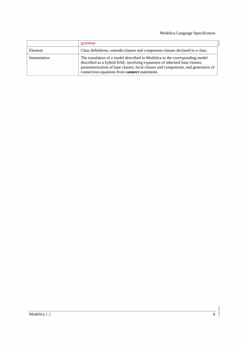
Element Class definitions, extends-clauses and component-clauses declared in a class.
Instantiation The translation of a model described in Modelica to the corresponding modeldescribed as a hybrid DAE, involving expansion of inherited base classes,parameterization of base classes, local classes and components, and generation ofconnection equations from connect statements
Modelica Language Specification
Modelica 1.2 7
2 Modelica syntax
2.1 Lexical conventions
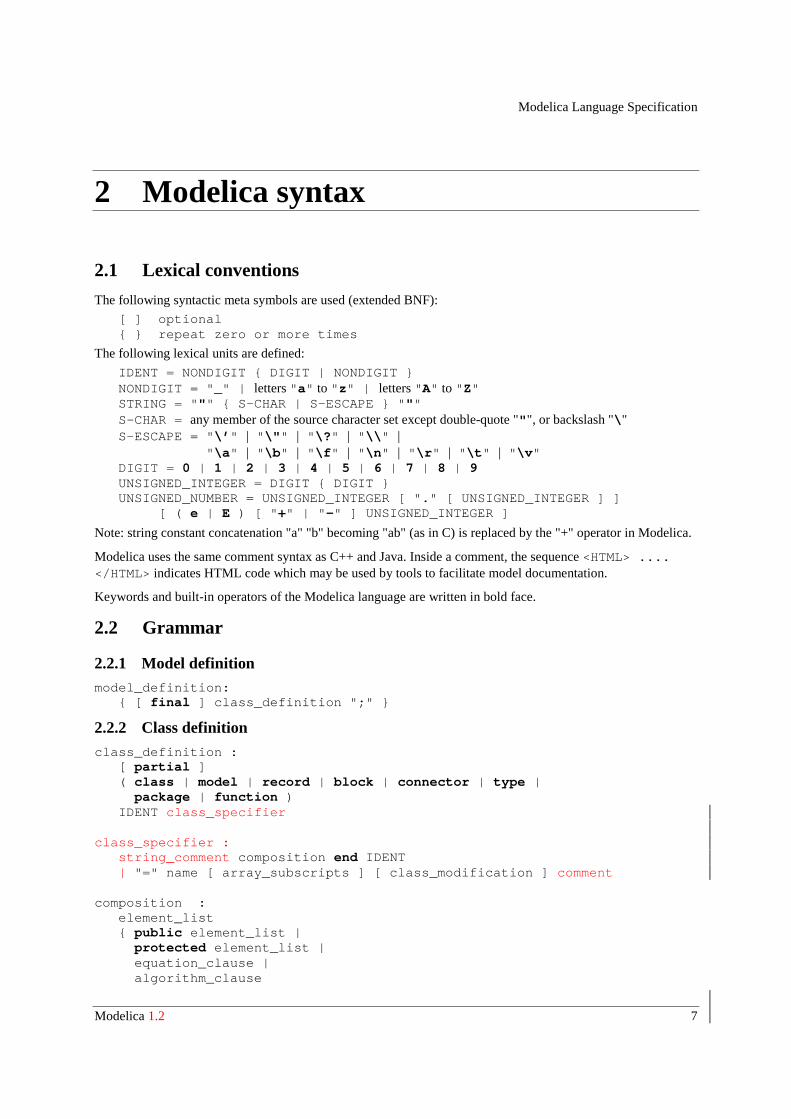
The following syntactic meta symbols are used (extended BNF):
[ ] optional{ } repeat zero or more times
The following lexical units are defined:
IDENT = NONDIGIT { DIGIT | NONDIGIT }NONDIGIT = "_" | letters "a" to "z" | letters "A" to "Z"STRING = """ { S-CHAR | S-ESCAPE } """S-CHAR = any member of the source character set except double-quote """, or backslash "\"S-ESCAPE = "\’ " | "\" " | "\? " | "\\ " | "\a " | "\b " | "\f " | "\n " | "\r " | "\t " | "\v "DIGIT = 0 | 1 | 2 | 3 | 4 | 5 | 6 | 7 | 8 | 9UNSIGNED_INTEGER = DIGIT { DIGIT }UNSIGNED_NUMBER = UNSIGNED_INTEGER [ ". " [ UNSIGNED_INTEGER ] ]
[ ( e | E ) [ "+" | "- " ] UNSIGNED_INTEGER ]
Note: string constant concatenation "a" "b" becoming "ab" (as in C) is replaced by the "+" operator in Modelica.
Modelica uses the same comment syntax as C++ and Java. Inside a comment, the sequence <HTML> ....</HTML> indicates HTML code which may be used by tools to facilitate model documentation.
Keywords and built-in operators of the Modelica language are written in bold face.
2.2 Grammar
2.2.1 Model definitionmodel_definition: { [ final ] class_definition ";" }
2.2.2 Class definition
class_definition : [ partial ] ( class | model | record | block | connector | type | package | function ) IDENT class_specifier
class_specifier : string_comment composition end IDENT | "=" name [ array_subscripts ] [ class_modification ] comment
composition : element_list { public element_list | protected element_list | equation_clause | algorithm_clause
Modelica Language Specification
Modelica 1.2 8
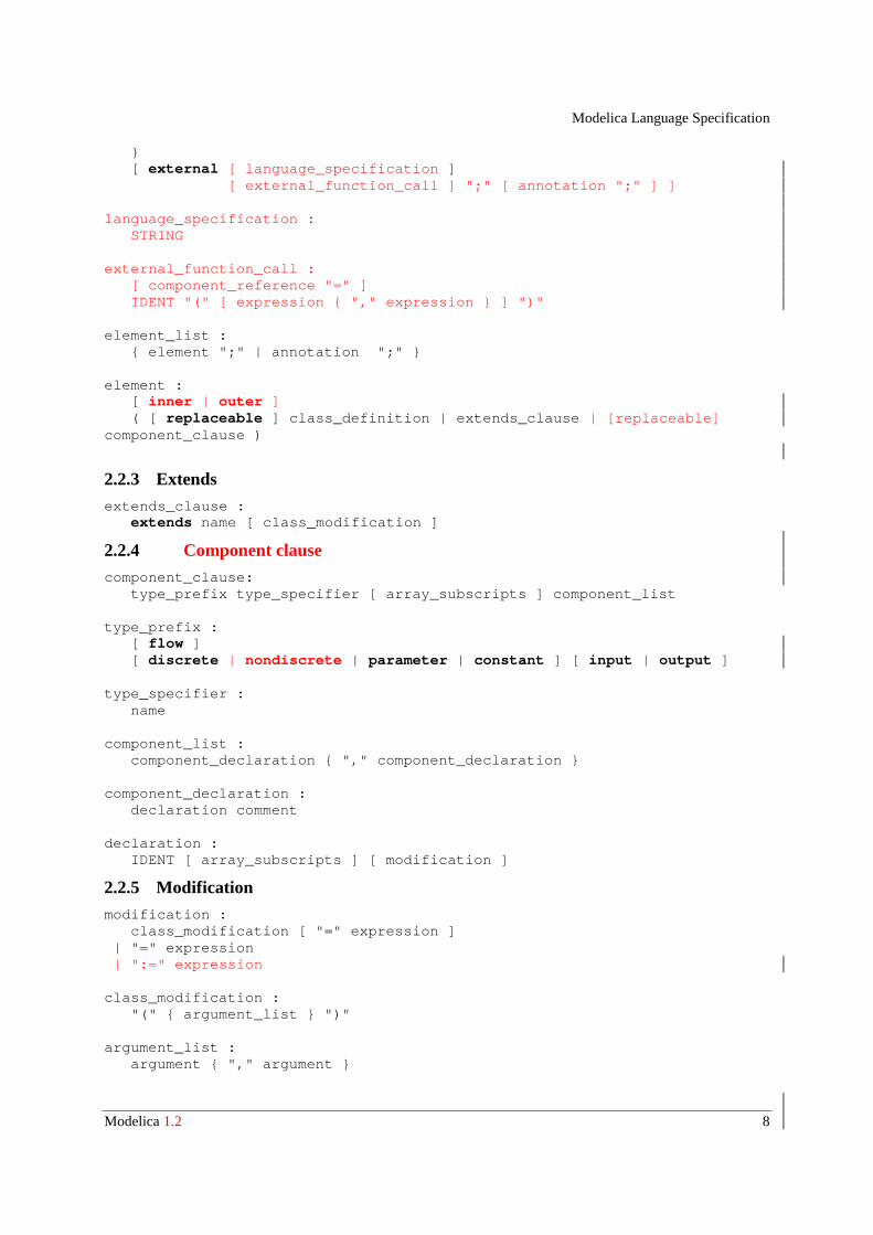
} [ external [ language_specification ] [ external_function_call ] ";" [ annotation ";" ] ]
language_specification : STRING
external_function_call : [ component_reference "=" ] IDENT "(" [ expression { "," expression } ] ")"
element_list : { element ";" | annotation ";" }
element : [ inner | outer ] ( [ replaceable ] class_definition | extends_clause | [replaceable]component_clause )
2.2.3 Extends
extends_clause : extends name [ class_modification ]
2.2.4 Component clause
component_clause: type_prefix type_specifier [ array_subscripts ] component_list
type_prefix : [ flow ] [ discrete | nondiscrete | parameter | constant ] [ input | output ]
type_specifier : name
component_list : component_declaration { "," component_declaration }
component_declaration : declaration comment
declaration : IDENT [ array_subscripts ] [ modification ]
2.2.5 Modification
modification : class_modification [ "=" expression ] | "=" expression | ":=" expression class_modification : "(" { argument_list } ")"
argument_list : argument { "," argument }
Modelica Language Specification
Modelica 1.2 9
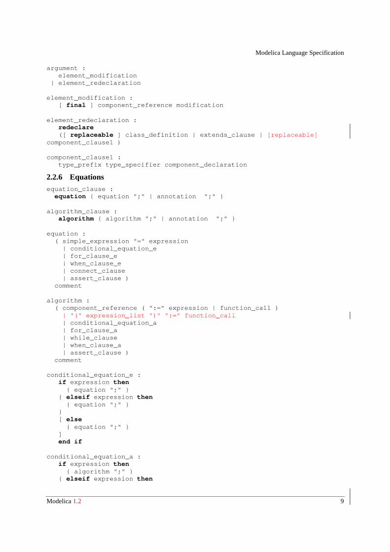
argument : element_modification | element_redeclaration
element_modification : [ final ] component_reference modification
element_redeclaration : redeclare ([ replaceable ] class_definition | extends_clause | [replaceable]component_clause1 )
component_clause1 : type_prefix type_specifier component_declaration
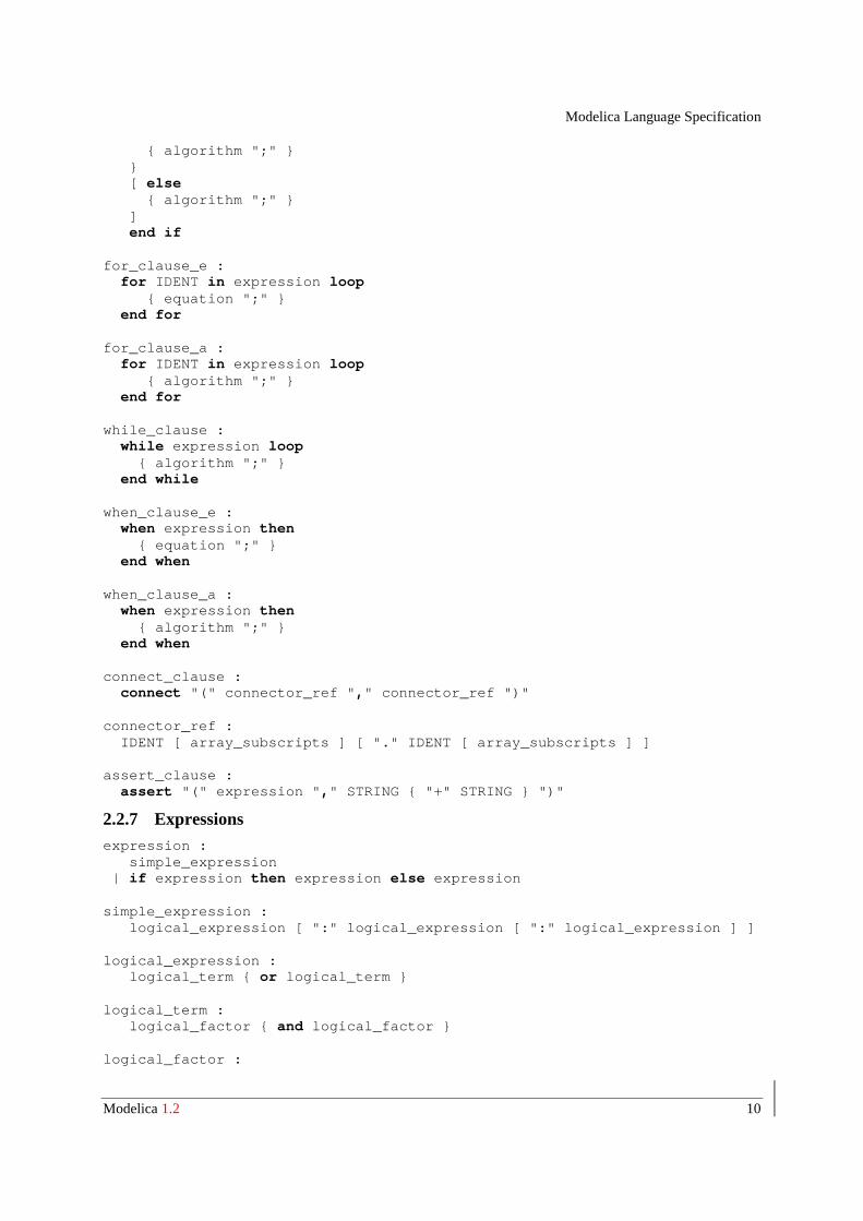
2.2.6 Equations
equation_clause : equation { equation ";" | annotation ";" }
algorithm_clause : algorithm { algorithm ";" | annotation ";" }
equation : ( simple_expression "=" expression | conditional_equation_e | for_clause_e | when_clause_e | connect_clause | assert_clause ) comment
algorithm : ( component_reference ( ":=" expression | function_call ) | "(" expression_list ")" ":=" function_call | conditional_equation_a | for_clause_a | while_clause | when_clause_a | assert_clause ) comment
conditional_equation_e : if expression then { equation ";" } { elseif expression then { equation ";" } } [ else { equation ";" } ] end if
conditional_equation_a : if expression then { algorithm ";" } { elseif expression then
Modelica Language Specification
Modelica 1.2 10
{ algorithm ";" } } [ else { algorithm ";" } ] end if
for_clause_e : for IDENT in expression loop { equation ";" } end for
for_clause_a : for IDENT in expression loop { algorithm ";" } end for
while_clause : while expression loop { algorithm ";" } end while
when_clause_e : when expression then { equation ";" } end when
when_clause_a : when expression then { algorithm ";" } end when
connect_clause : connect "(" connector_ref "," connector_ref ")"
connector_ref : IDENT [ array_subscripts ] [ "." IDENT [ array_subscripts ] ]
assert_clause : assert "(" expression "," STRING { "+" STRING } ")"
2.2.7 Expressionsexpression : simple_expression | if expression then expression else expression
simple_expression : logical_expression [ ":" logical_expression [ ":" logical_expression ] ]
logical_expression : logical_term { or logical_term }
logical_term : logical_factor { and logical_factor }
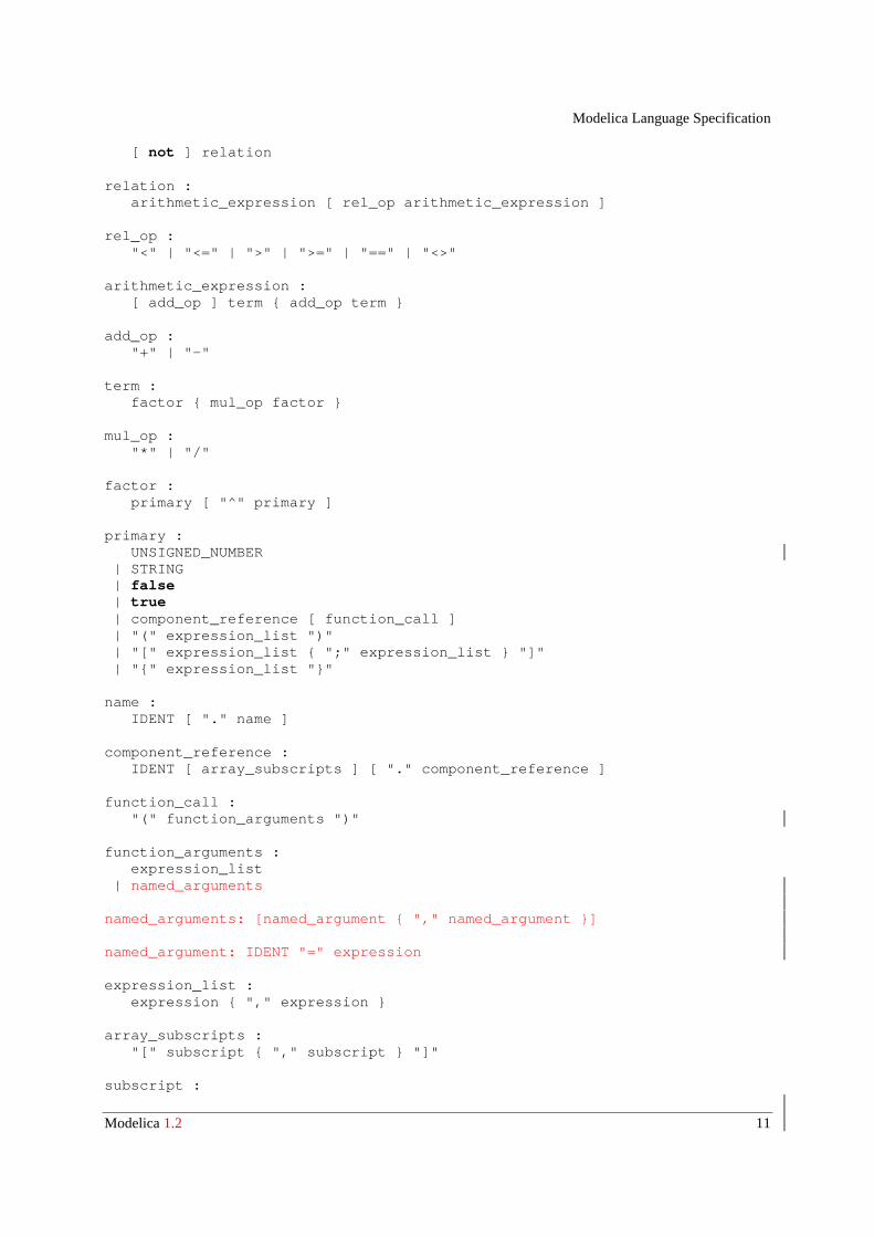
logical_factor :
Modelica Language Specification
Modelica 1.2 11
[ not ] relation
relation : arithmetic_expression [ rel_op arithmetic_expression ]
rel_op : "<" | "<=" | ">" | ">=" | "==" | "<>"
arithmetic_expression : [ add_op ] term { add_op term }
add_op : "+" | "-"
term : factor { mul_op factor }
mul_op : "*" | "/"
factor : primary [ "^" primary ]
primary : UNSIGNED_NUMBER | STRING | false | true | component_reference [ function_call ] | "(" expression_list ")" | "[" expression_list { ";" expression_list } "]" | "{" expression_list "}"
name : IDENT [ "." name ]
component_reference : IDENT [ array_subscripts ] [ "." component_reference ]
function_call : "(" function_arguments ")"
function_arguments : expression_list | named_arguments
named_arguments: [named_argument { "," named_argument }]
named_argument: IDENT "=" expression
expression_list : expression { "," expression }
array_subscripts : "[" subscript { "," subscript } "]"
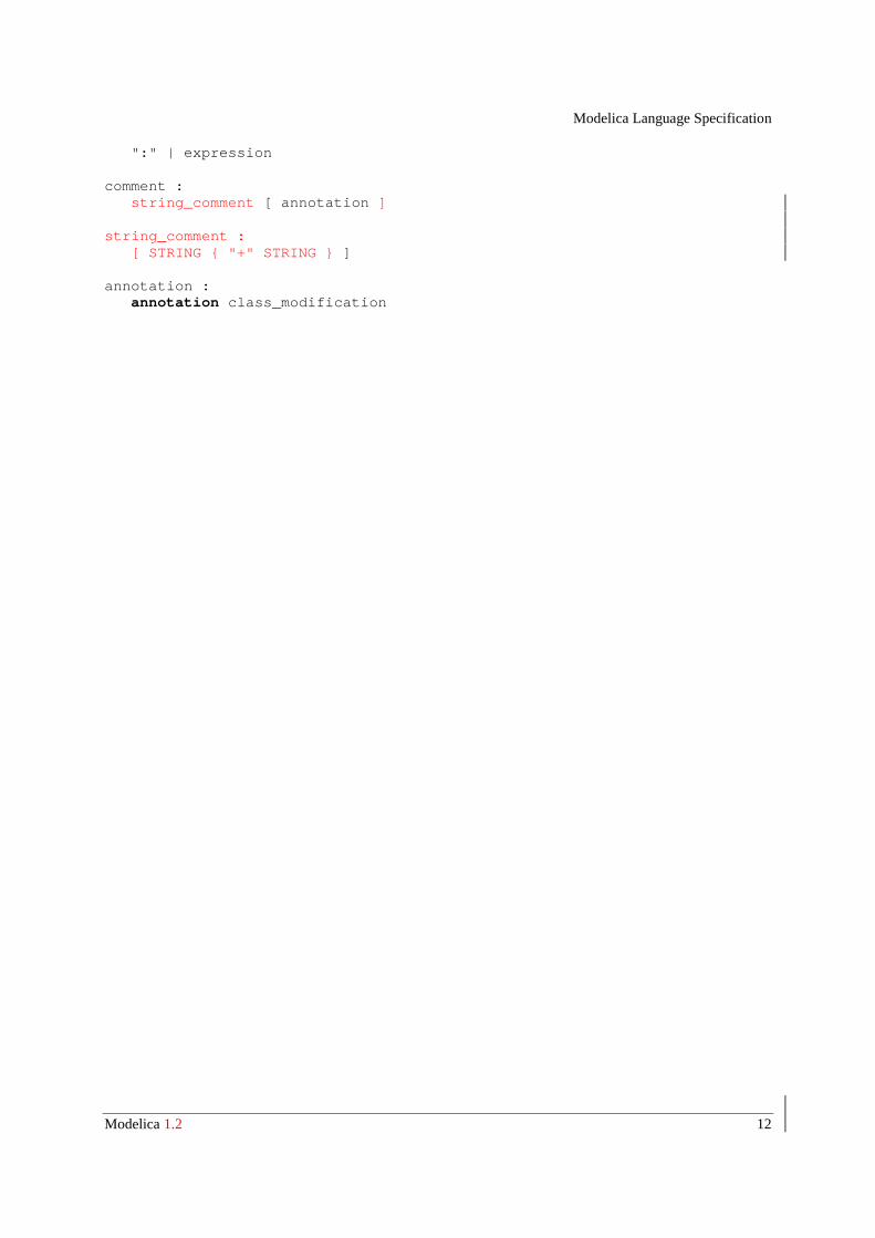
subscript :
Modelica Language Specification
Modelica 1.2 12
":" | expression
comment : string_comment [ annotation ]
string_comment : [ STRING { "+" STRING } ]
annotation : annotation class_modification
Modelica Language Specification
Modelica 1.2 13
3 Modelica semantics
3.1 Fundamentals
Instantiation is made in a context which consists of an environment and an ordered set of parents.
3.1.1 Scoping and name lookup
3.1.1.1 Parents
The classes lexically enclosing an element form an ordered set of parents. A class defined inside another classdefinition (the parent) preceeds its enclosing class definition in this set.
Enclosing all class definitions is an unnamed parent which contains all top-level class definitions. The order oftop-level class definitions in the unnamed parent is undefined.
During instantiation, the parent of an element being instantiated is a partially instantiated class. [For example,this means that a declaration can refer to a name previously inherited through a previous extends clause.]
[Example:
class C1 ... end C1;class C2 ... end C2;class C3 Real x=3; C1 y; class C4 Real z; end C4;end C3;
The unnamed parent of class definition C3 contains C1 and C2 in arbitrary order. When instantiating classdefinition C3, the set of parents of the declaration of x is the partially instantiated class C3 followed by theunnamed parent with C1 and C2. The set of parents of z are C4, C3 and the unnamed parent in that order.]
3.1.1.2 Static name lookup
Names are looked up at class instantiation to find names of base classes, component types, etc.
For a simple name [not composed using dot-notation] lookup is performed as follows:
• When an element, equation or algorithm is instantiated, any name is looked up sequentially in each memberof the ordered set of parents until a match is found.
For a composite name of the form A.B [or A.B.C, etc.] lookup is performed as follows:
• The first identifier [A] is looked up as defined above.
• If the identifier denotes a component, the rest of the name [e.g., B or B.C] is looked up in the component.
• If the identifier denotes a class, that class is temporarily instantiated with an empty environment and usingthe parents of the denoted class. The rest of the name [e.g., B or B.C] is looked up in the temporaryinstantiated class.
[The temporary class instantiation performed for composite names follow the same rules as class instantiation ofthe base class in an extends clause, local classes and the type in a component clause, except that the
Modelica Language Specification
Modelica 1.2 14
environment is empty.]
All parts of a composite name denoting a component shall denote components. [There are no class variables inModelica.]
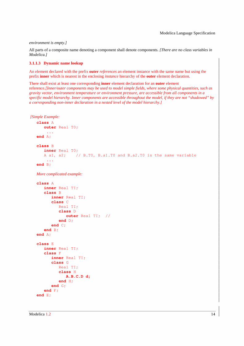
3.1.1.3 Dynamic name lookup
An element declared with the prefix outer references an element instance with the same name but using theprefix inner which is nearest in the enclosing instance hierarchy of the outer element declaration.
There shall exist at least one corresponding inner element declaration for an outer elementreference.[Inner/outer components may be used to model simple fields, where some physical quantities, such asgravity vector, environment temperature or environment pressure, are accessible from all components in aspecific model hierarchy. Inner components are accessible throughout the model, if they are not “shadowed” bya corresponding non-inner declaration in a nested level of the model hierarchy.]
[Simple Example:
class A outer Real T0; ...end A;
class B inner Real T0; A a1, a2; // B.T0, B.a1.T0 and B.a2.T0 is the same variable ...end B;
More complicated example:
class A inner Real TI; class B inner Real TI; class C Real TI; class D outer Real TI; // end D; end C; end B;end A;
class E inner Real TI; class F inner Real TI; class G Real TI; class H A.B.C.D d; end H; end G; end F;end E;
Modelica Language Specification
Modelica 1.2 15
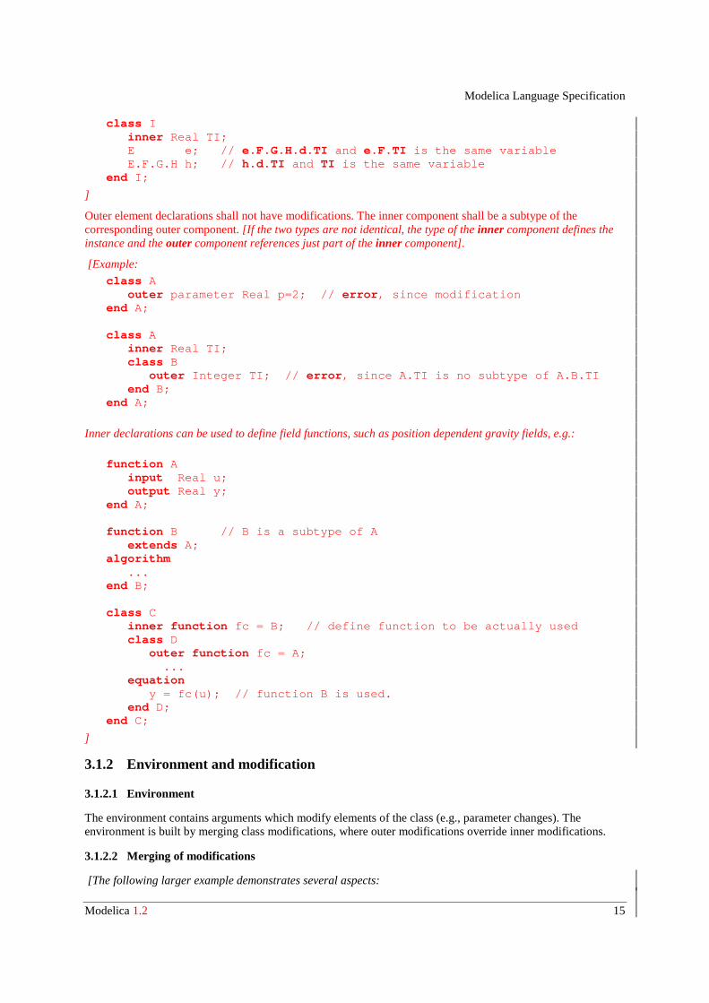
class I inner Real TI; E e; // e.F.G.H.d.TI and e.F.TI is the same variable E.F.G.H h; // h.d.TI and TI is the same variableend I;
]
Outer element declarations shall not have modifications. The inner component shall be a subtype of thecorresponding outer component. [If the two types are not identical, the type of the inner component defines theinstance and the outer component references just part of the inner component].
[Example:
class A outer parameter Real p=2; // error, since modificationend A;
class A inner Real TI; class B outer Integer TI; // error, since A.TI is no subtype of A.B.TI end B;end A;
Inner declarations can be used to define field functions, such as position dependent gravity fields, e.g.:
function A input Real u; output Real y;end A;
function B // B is a subtype of A extends A;algorithm ...end B;
class C inner function fc = B; // define function to be actually used class D outer function fc = A; ... equation y = fc(u); // function B is used. end D;end C;
]
3.1.2 Environment and modification
3.1.2.1 Environment
The environment contains arguments which modify elements of the class (e.g., parameter changes). Theenvironment is built by merging class modifications, where outer modifications override inner modifications.
3.1.2.2 Merging of modifications
[The following larger example demonstrates several aspects:
Modelica Language Specification
Modelica 1.2 16
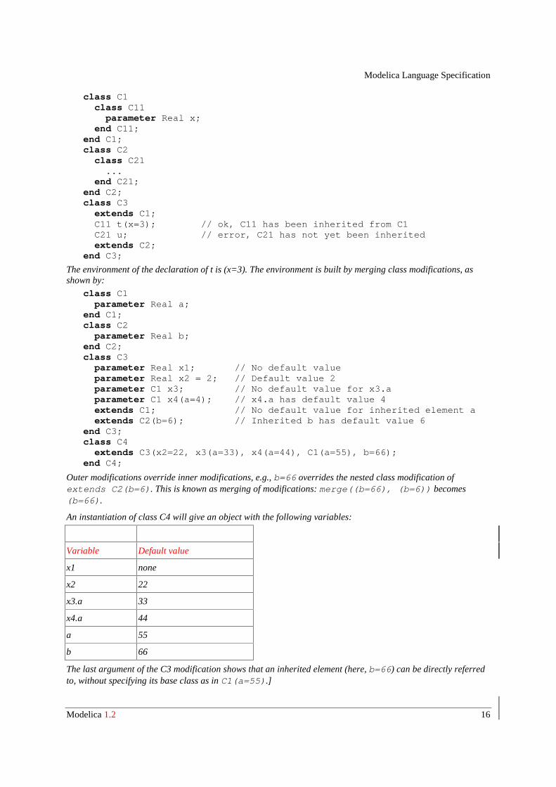
class C1 class C11 parameter Real x; end C11; end C1;class C2 class C21 ... end C21; end C2;class C3 extends C1; C11 t(x=3); // ok, C11 has been inherited from C1 C21 u; // error, C21 has not yet been inherited extends C2;end C3;
The environment of the declaration of t is (x=3). The environment is built by merging class modifications, asshown by:
class C1 parameter Real a; end C1;class C2 parameter Real b; end C2;class C3 parameter Real x1; // No default value parameter Real x2 = 2; // Default value 2 parameter C1 x3; // No default value for x3.a parameter C1 x4(a=4); // x4.a has default value 4 extends C1; // No default value for inherited element a extends C2(b=6); // Inherited b has default value 6end C3;class C4 extends C3(x2=22, x3(a=33), x4(a=44), C1(a=55), b=66);end C4;
Outer modifications override inner modifications, e.g., b=66 overrides the nested class modification ofextends C2(b=6). This is known as merging of modifications: merge((b=66), (b=6)) becomes(b=66).
An instantiation of class C4 will give an object with the following variables:
Variable Default value
x1 none
x2 22
x3.a 33
x4.a 44
a 55
b 66
The last argument of the C3 modification shows that an inherited element (here, b=66) can be directly referredto, without specifying its base class as in C1(a=55).]
Modelica Language Specification
Modelica 1.2 17
3.1.2.3 Single modification
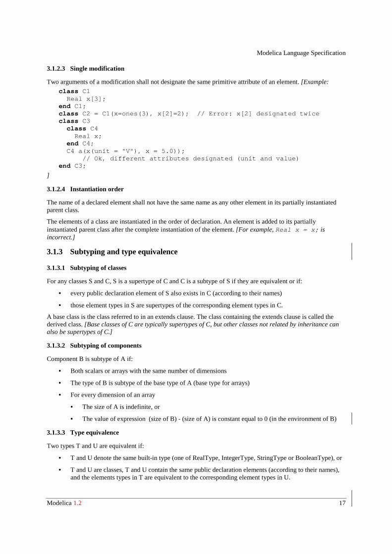
Two arguments of a modification shall not designate the same primitive attribute of an element. [Example:
class C1 Real x[3];end C1;class C2 = C1(x=ones(3), x[2]=2); // Error: x[2] designated twiceclass C3 class C4 Real x; end C4; C4 a(x(unit = "V"), x = 5.0)); // Ok, different attributes designated (unit and value)end C3;
]
3.1.2.4 Instantiation order
The name of a declared element shall not have the same name as any other element in its partially instantiatedparent class.
The elements of a class are instantiated in the order of declaration. An element is added to its partiallyinstantiated parent class after the complete instantiation of the element. [For example, Real x = x; isincorrect.]
3.1.3 Subtyping and type equivalence
3.1.3.1 Subtyping of classes
For any classes S and C, S is a supertype of C and C is a subtype of S if they are equivalent or if:
• every public declaration element of S also exists in C (according to their names)
• those element types in S are supertypes of the corresponding element types in C.
A base class is the class referred to in an extends clause. The class containing the extends clause is called thederived class. [Base classes of C are typically supertypes of C, but other classes not related by inheritance canalso be supertypes of C.]
3.1.3.2 Subtyping of components
Component B is subtype of A if:
• Both scalars or arrays with the same number of dimensions
• The type of B is subtype of the base type of A (base type for arrays)
• For every dimension of an array
• The size of A is indefinite, or
• The value of expression (size of B) - (size of A) is constant equal to 0 (in the environment of B)
3.1.3.3 Type equivalence
Two types T and U are equivalent if:
• T and U denote the same built-in type (one of RealType, IntegerType, StringType or BooleanType), or
• T and U are classes, T and U contain the same public declaration elements (according to their names),and the elements types in T are equivalent to the corresponding element types in U.
Modelica Language Specification
Modelica 1.2 18
3.1.3.4 Type identity
Two elements T and U are identical if:
• T and U are equivalent,
• they are either both declared as final or none is declared final,
• for a component their type prefixes are identical, and
• if T and U are classes, T and U contain the same public declaration elements (according to their names),and the elements in T are identical to the corresponding element in U.
3.1.4 Classes on external files
Class names are automatically mapped to a hierarchical structure of the operating system. Given that A denotes aclass at global scope, the name path A.B.C is looked up as follows.
• If A is defined in the current translation unit, the rest of the path (B.C) is looked up inside A.
• Otherwise, A is located in an ordered list of library roots, called MODELICAPATH.
If the name A is a structured entity [e.g. a directory], lookup of B.C progresses recursively in A.
If the name A is a non-structured entity [e.g. a file], it shall contain only the complete definition of class A, andthe rest of the path (B.C) is looked up inside that entity. If the name A is a structured entity [e.g. a directory withan optional node], the rest of the path is looked up in the node in the same way as in non-structured entity . If notfound, lookup of B.C progresses recursively in A.
[In a file hierarchy, the node is stored in file package.mo in the package directory].
Otherwise the lookup fails.
[On a typical system, MODELICAPATH is an environment variable containing a semicolon-separated list ofdirectory names. Classes are realized by directories with subdirectories, or files containing class definitions.The default file extension for Modelica is .mo; for example, the package A would be stored in file A.mo. Ifthere is both a subdirectory A and a file A.mo, the lookup fails. Other forms of realizing packages are alsopossible, for example using a hierarchical database.]
[The first part of the path A.B.C (i.e., A) is located by searching the ordered list of roots in MODELICAPATH.If no root contains A the lookup fails. If A has been found in one of the roots, the rest of the path is located in A;if that fails, the entire lookup fails without searching for A in any of the remaining roots in MODELICAPATH.]
3.2 Declarations
3.2.1 Component clause
If the type specifier of the component denotes a built-in type (RealType, IntegerType, etc.), the instantiatedcomponent has the same type.
If the type specifier of the component does not denote a built-in type, the name of the type is looked up (3.1.1).The found type is instantiated with a new environment and the partially instantiated parent of the component.The new environment is the result of merging
• the modification of parent element-modification with the same name as the component
• the modification of the component declaration
in that order.
An environment that defines the value of a component of built-in type is said to define a declaration equationassociated with the declared component. For declarations of vectors and matrices, declaration equations areassociated with each element. [This makes it possible to override the declaration equation for a single element in
Modelica Language Specification
Modelica 1.2 19
a parent modelification, which would not be possible if the declaration equation is regarded as a single matrixequation.]
Array dimensions shall be non-negative parameter expressions.
Variables declared with the flow type prefix shall be a subtype of Real.
Type prefixes (i.e., flow, discrete, nondiscrete, parameter, constant, input, output) shall only be applied for type,record and connector components. Type prefixes of a structured component are also applied to the elements ofthe component. Type prefixes shall only be applied for a structured component, if no element of the componenthas a corresponding type prefix of the same category. [For example, input can only be used, if none of theelements has an input or output type prefix].
Components of function type may be instantiated. [A modifier can be used to e.g. change parameters of thefunction. It is also possible to do such a modification with a class specialization.] Components of a function donot have start-attributes, but a binding assignment (":=" expression) is an expression such that the component isinitialized to this expression at the start of every function invocation (before executing the algorithm section orcalling the external function). Binding assignments can only be used for components of a function. If no bindingassignment is given for a non-input component its value at the start of the function invocation is undefined. It isa quality of implementation issue to diagnose this for non-external functions. The size of each non-input arraycomponent of a function must be given by the inputs. Components of a function will inside the function behaveas though they had discrete variability.
3.2.2 Variability prefix
The prefixes nondiscrete, discrete, parameter, constant of a component declaration are called variabilityprefixes and define in which situation the variable values of a component are initialized (see section 3.6) andwhen they are changed in transient analysis (= solution of initial value problem of the hybrid DAE):
• Parameter and constant variables vc remain constant during transient analysis (vc=const.).
• Discrete variables vd are discrete-time variables, i.e., they have a vanishing time derivative (der(vd)=0) andcan change their values only at event instants during transient analysis (see section 3.7).
• Nondiscrete variables vn are continuous-time variables, i.e., they may have a non-vanishing time derivative(der(vn)≠0 possible) and may change their values at any time during transient analysis (see section 3.7).
If no variability prefix is present in a declaration, the following default variability is used for the variables of thecomponent according to their base types:
base type default variability comment
Real nondiscrete continuous-time variable
Boolean, Integer, String discrete discrete-time variable
[A discrete variable is a piecewise constant signal which changes its values only at event instants duringsimulation. This prefix is needed in order that special algorithms, such as the algorithm of Pantelides for indexreduction, can be applied (it must be known that the time derivative of these variables is identical to zero).Furthermore, memory requirements can be reduced in the simulation environment, if it is known that acomponent can only change at event instants.
A parameter variable is constant during simulation. This prefix gives the library designer the possibility toexpress that the physical equations in a library are only valid if some of the used components are constantduring simulation. The same also holds for the discrete and constant prefix. Additionally, the parameter prefixallows a convenient graphical user interface in an experiment environment, to support quick changes of the mostimportant constants of a compiled model. In combination with an if-clause, a parameter prefix allows to removeparts of a model before the symbolic processing of a model takes place in order to avoid variable causalities inthe model (similar to #ifdef in C). Class parameters can be sometimes used as an alternative. Example:
model Inertia parameter Boolean state = true; ...
Modelica Language Specification
Modelica 1.2 20
equation J*a = t1 - t2; if state then // code which is removed during symbolic der(v) = a; // processing, if state=false der(r) = v; end ifend Inertia;
A constant variable is similar to a parameter with the difference that constants cannot be changed after theyhave been declared. It can be used to represent mathematical constants, e.g.
constant Real PI=4*arctan(1);
A nondiscrete Boolean is a continuous-time variable, i.e., its value can change during continuous integration.This type is needed in some rare cases:
Boolean off1, off1a; nondiscrete Boolean off2; equation off1 = s1 < 0; off1a = noEvent(s1 < 0); // error, since off1a is discrete off2 = noEvent(s2 < 0); // possible, because nondiscrete variable u1 = if off1 then s1 else 0; // state events u2 = if off2 then s2 else 0; // no state events
Since off1 is a discrete variable, state events are generated such that off1 is only changed at event instants.Variable off2 may change its value during continuous integration. As a result, u1 is guaranteed to be continuousduring continuous integration whereas no such guarantee exists for u2.
]
3.2.3 Expressions
Constant expressions are:
• Real, Integer, Boolean and String literals.
• Real, Integer, Boolean and String variables declared as constant .
• Except for the special built-in operators initial, terminal, der, edge, sample, pre and analysisType afunction or operator with constant subexpressions as argument (and no parameters defined in thefunction) is a constant expression.
Parameter expressions are:
• Constant expressions.
• Real, Integer, Boolean and String variables declared as parameter.
• Except for the special built-in operators initial, terminal, der, edge, sample and pre a function oroperator with parameter subexpressions is a parameter expression.
• The function analysisType() is parameter expression.
Discrete expressions are:
• Parameter expressions.
• Real, Integer, Boolean and String variables declared as discrete.
• Function calls where all input arguments of the function are discrete expressions.
• Expressions where all the subexpressions are discrete expressions.
Modelica Language Specification
Modelica 1.2 21
• Expressions in the body of a when clause.
• The result of comparing a nondiscrete Real with a numeric value.
• The functions pre, edge, and change result in discrete expressions.
• Expressions in functions behave as though they were discrete expressions.
If the value of a constant or parameter expression is either directly or indirectly used as structural expression (i.e.to compute the size of a component or for if-statements with unequal sizes of the branches) it is a quality-of-implementation issue whether any calls of non-builtin functions are allowed as subexpressions. [The intention isto erase this restriction for Modelica 2.0.]
Components declared as constant shall have an associated declaration equation with a constant expression. Thevalue of a constant cannot be changed after its declaration.
The declaration equation of a parameter component and of the base type attributes [such as start] needs to be aparameter expression.
The declaration equation of a discrete component needs to be a discrete expression.[Example:
model Constants parameter Real p1 = 1; constant Real c1 = p1 + 2; // error, no constant expression parameter Real p2 = p1 + 2;end Constants;
model Test Constants c1(p1=3); // fine Constants c2(p2=7); // fine, declaration equation can be modifiedend Test;
]
3.2.4 Vectors, Matrices, and Arrays
3.2.4.1 Array declarations
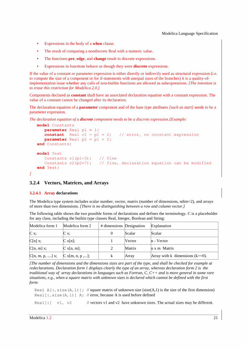
The Modelica type system includes scalar number, vector, matrix (number of dimensions, ndim=2), and arraysof more than two dimensions. [There is no distinguishing between a row and column vector.]
The following table shows the two possible forms of declarations and defines the terminology. C is a placeholderfor any class, including the builtin type classes Real, Integer, Boolean and String:
Modelica form 1 Modelica form 2 # dimensions Designation Explanation
C x; C x; 0 Scalar Scalar
C[n] x; C x[n]; 1 Vector n - Vector
C[n, m] x; C x[n, m]; 2 Matrix n x m Matrix
C[n, m, p, ....] x; C x[m, n, p ,...]; k Array Array with k dimensions (k>=0).
[The number of dimensions and the dimensions sizes are part of the type, and shall be checked for example atredeclarations. Declaration form 1 displays clearly the type of an array, whereas declaration form 2 is thetraditional way of array declarations in languages such as Fortran, C, C++ and is more general in some raresituations, e.g., when a square matrix with unknown sizes is declared which cannot be defined with the firstform:
Real A[:,size(A,1)]; // square matrix of unknown size (size(A,1) is the size of the first dimension) Real[:,size(A,1)] A; // error, because A is used before defined
Real[:] v1, v2 // vectors v1 and v2 have unknown sizes. The actual sizes may be different.
Modelica Language Specification
Modelica 1.2 22
It is possible to mix the two declaration forms, but it is not recommended
Real[3,2] x[4,5]; // x has type Real[4,5,3,2];]
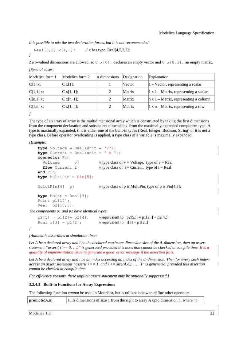
Zero-valued dimensions are allowed, so C x[0]; declares an empty vector and C x[0,3]; an empty matrix.
[Special cases:
Modelica form 1 Modelica form 2 # dimensions Designation Explanation
C[1] x; C x[1]; 1 Vector 1 – Vector, representing a scalar
C[1,1] x; C x[1, 1]; 2 Matrix 1 x 1 – Matrix, representing a scalar
C[n,1] x; C x[n, 1]; 2 Matrix n x 1 – Matrix, representing a column
C[1,n] x; C x[1, n]; 2 Matrix 1 x n – Matrix, representing a row
]
The type of an array of array is the multidimensional array which is constructed by taking the first dimensionsfrom the component declaration and subsequent dimensions from the maximally expanded component type. Atype is maximally expanded, if it is either one of the built-in types (Real, Integer, Boolean, String) or it is not atype class. Before operator overloading is applied, a type class of a variable is maximally expanded.
[Example:
type Voltage = Real(unit = "V");type Current = Real(unit = " A ");connector Pin Voltage v; // type class of v = Voltage, type of v = Real flow Current i; // type class of i = Current, type of i = Realend Pin;type MultiPin = Pin[5];
MultiPin[4] p; // type class of p is MultiPin, type of p is Pin[4,5];
type Point = Real[3];Point p1[10];Real p2[10,3];
The components p1 and p2 have identical types.
p2[5] = p1[2]+ p2[4]; // equivalent to p2[5,:] = p1[2,:] + p2[4,:]Real r[3] = p1[2]; // equivalent to r[3] = p1[2,:]
]
[Automatic assertions at simulation time:
Let A be a declared array and i be the declared maximum dimension size of the di-dimension, then an assertstatement “assert( i >= 0, …)” is generated provided this assertion cannot be checked at compile time. It is aqualitity of implementation issue to generate a good error message if the assertion fails.
Let A be a declared array and i be an index accessing an index of the di-dimension. Then for every such index-access an assert statement “assert( i >= 1 and i <= size(A,di),, … )” is generated, provided this assertioncannot be checked at compile time.
For efficiency reasons, these implicit assert statement may be optionally suppressed.]
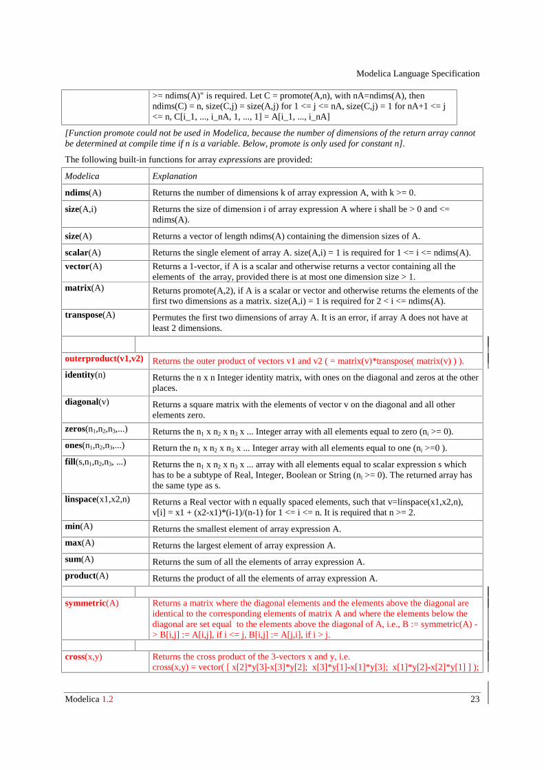
3.2.4.2 Built-in Functions for Array Expressions
The following function cannot be used in Modelica, but is utilized below to define other operators
promote(A,n) Fills dimensions of size 1 from the right to array A upto dimension n, where "n
Modelica Language Specification
Modelica 1.2 23
>= ndims(A)" is required. Let C = promote(A,n), with nA=ndims(A), thenndims(C) = n, size(C,j) = size(A,j) for 1 <= j <= nA, size(C,j) = 1 for nA+1 <= j<= n, C[i_1, ..., i_nA, 1, ..., 1] = A[i_1, ..., i_nA]
[Function promote could not be used in Modelica, because the number of dimensions of the return array cannotbe determined at compile time if n is a variable. Below, promote is only used for constant n].
The following built-in functions for array expressions are provided:
Modelica Explanation
ndims(A) Returns the number of dimensions k of array expression A, with k >= 0.
size(A,i) Returns the size of dimension i of array expression A where i shall be > 0 and <=ndims(A).
size(A) Returns a vector of length ndims(A) containing the dimension sizes of A.
scalar(A) Returns the single element of array A. size(A,i) = 1 is required for 1 <= i <= ndims(A).
vector(A) Returns a 1-vector, if A is a scalar and otherwise returns a vector containing all theelements of the array, provided there is at most one dimension size > 1.
matrix(A) Returns promote(A,2), if A is a scalar or vector and otherwise returns the elements of thefirst two dimensions as a matrix. size(A,i) = 1 is required for 2 < i <= ndims(A).
transpose(A) Permutes the first two dimensions of array A. It is an error, if array A does not have atleast 2 dimensions.
outerproduct(v1,v2) Returns the outer product of vectors v1 and v2 ( = matrix(v)*transpose( matrix(v) ) ).
identity(n) Returns the n x n Integer identity matrix, with ones on the diagonal and zeros at the otherplaces.
diagonal(v) Returns a square matrix with the elements of vector v on the diagonal and all otherelements zero.
zeros(n1,n2,n3,...) Returns the n1 x n2 x n3 x ... Integer array with all elements equal to zero (ni >= 0).
ones(n1,n2,n3,...) Return the n1 x n2 x n3 x ... Integer array with all elements equal to one (ni >=0 ).
fill(s,n1,n2,n3, ...) Returns the n1 x n2 x n3 x ... array with all elements equal to scalar expression s whichhas to be a subtype of Real, Integer, Boolean or String (ni >= 0). The returned array hasthe same type as s.
linspace(x1,x2,n) Returns a Real vector with n equally spaced elements, such that v=linspace(x1,x2,n),v[i] = x1 + (x2-x1)*(i-1)/(n-1) for 1 <= i <= n. It is required that n >= 2.
min(A) Returns the smallest element of array expression A.
max(A) Returns the largest element of array expression A.
sum(A) Returns the sum of all the elements of array expression A.
product(A) Returns the product of all the elements of array expression A.
symmetric(A) Returns a matrix where the diagonal elements and the elements above the diagonal areidentical to the corresponding elements of matrix A and where the elements below thediagonal are set equal to the elements above the diagonal of A, i.e., B := symmetric(A) -> B[i,j] := A[i,j], if i <= j, B[i,j] := A[j,i], if i > j.
cross(x,y) Returns the cross product of the 3-vectors x and y, i.e.cross(x,y) = vector( [ x[2]*y[3]-x[3]*y[2]; x[3]*y[1]-x[1]*y[3]; x[1]*y[2]-x[2]*y[1] ] );
Modelica Language Specification
Modelica 1.2 24
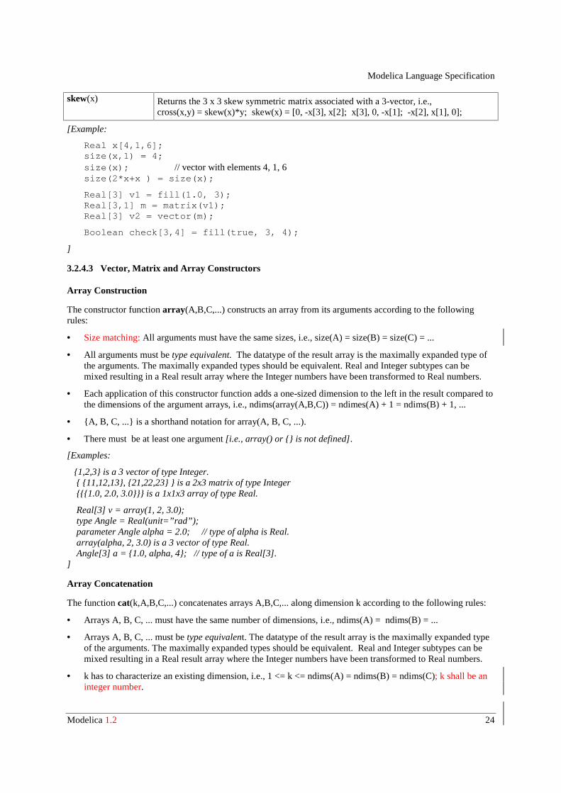
skew(x) Returns the 3 x 3 skew symmetric matrix associated with a 3-vector, i.e.,cross(x,y) = skew(x)*y; skew(x) = [0, -x[3], x[2]; x[3], 0, -x[1]; -x[2], x[1], 0];
[Example:
Real x[4,1,6]; size(x,1) = 4; size(x); // vector with elements 4, 1, 6 size(2*x+x ) = size(x);
Real[3] v1 = fill(1.0, 3); Real[3,1] m = matrix(v1); Real[3] v2 = vector(m);
Boolean check[3,4] = fill(true, 3, 4);
]
3.2.4.3 Vector, Matrix and Array Constructors
Array Construction
The constructor function array(A,B,C,...) constructs an array from its arguments according to the followingrules:
• Size matching: All arguments must have the same sizes, i.e., size(A) = size(B) = size(C) = ...
• All arguments must be type equivalent. The datatype of the result array is the maximally expanded type ofthe arguments. The maximally expanded types should be equivalent. Real and Integer subtypes can bemixed resulting in a Real result array where the Integer numbers have been transformed to Real numbers.
• Each application of this constructor function adds a one-sized dimension to the left in the result compared tothe dimensions of the argument arrays, i.e., ndims(array(A,B,C)) = ndimes(A) + 1 = ndims(B) + 1, ...
• {A, B, C, ...} is a shorthand notation for array(A, B, C, ...).
• There must be at least one argument [i.e., array() or {} is not defined].
[Examples:
{1,2,3} is a 3 vector of type Integer. { {11,12,13}, {21,22,23} } is a 2x3 matrix of type Integer {{{1.0, 2.0, 3.0}}} is a 1x1x3 array of type Real.
Real[3] v = array(1, 2, 3.0); type Angle = Real(unit=”rad”); parameter Angle alpha = 2.0; // type of alpha is Real. array(alpha, 2, 3.0) is a 3 vector of type Real. Angle[3] a = {1.0, alpha, 4}; // type of a is Real[3].]
Array Concatenation
The function cat(k,A,B,C,...) concatenates arrays A,B,C,... along dimension k according to the following rules:
• Arrays A, B, C, ... must have the same number of dimensions, i.e., ndims(A) = ndims(B) = ...
• Arrays A, B, C, ... must be type equivalent. The datatype of the result array is the maximally expanded typeof the arguments. The maximally expanded types should be equivalent. Real and Integer subtypes can bemixed resulting in a Real result array where the Integer numbers have been transformed to Real numbers.
• k has to characterize an existing dimension, i.e., 1 <= k <= ndims(A) = ndims(B) = ndims(C); k shall be aninteger number.
Modelica Language Specification
Modelica 1.2 25
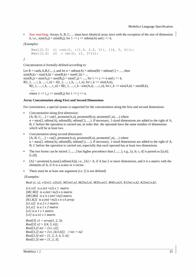
• Size matching: Arrays A, B, C, ... must have identical array sizes with the exception of the size of dimensionk, i.e., size(A,j) = size(B,j), for 1 <= j <= ndims(A) and j <> k.
[Examples:
Real[2,3] r1 =cat(1, {{1.0, 2.0, 3}}, {{4, 5, 6}}); Real[2,6] r2 = cat(2, r1, 2*r1);
]
Concatenation is formally defined according to:
Let R = cat(k,A,B,C,...), and let n = ndims(A) = ndims(B) = ndims(C) = ...., thensize(R,k) = size(A,k) + size(B,k) + size(C,k) + ...size(R,j) = size(A,j) = size(B,j) = size(C,j) = ...., for 1 <= j <= n and j <> k.R[i_1, ..., i_k, ..., i_n] = A[i_1, ..., i_k, ..., i_n], for i_k <= size(A,k), R[i_1, ..., i_k, ..., i_n] = B[i_1, ..., i_k - size(A,i), ..., i_n], for i_k <= size(A,k) + size(B,k), .... where 1 <= i_j <= size(R,j) for 1 <= j <= n.
Array Concatenation along First and Second Dimensions
For convenience, a special syntax is supported for the concatenation along the first and second dimensions.
• Concatenation along first dimension:[A; B; C; ...] = cat(1, promote(A,n), promote(B,n), promote(C,n), ...) wheren = max(2, ndims(A), ndims(B), ndims(C), ....). If necessary, 1-sized dimensions are added to the right of A,B, C before the operation is carried out, in order that the operands have the same number of dimensionswhich will be at least two.
• Concatenation along second dimension:[A, B, C, ...] = cat(2, promote(A,n), promote(B,n), promote(C,n), ...) wheren = max(2, ndims(A), ndims(B), ndims(C), ....). If necessary, 1-sized dimensions are added to the right of A,B, C before the operation is carried out, especially that each operand has at least two dimensions.
• The two forms can be mixed. [...,...] has higher precedence than [...;...], e.g., [a, b; c, d] is parsed as [[a,b];[c,d]].
• [A] = promote(A,max(2,ndims(A))), i.e., [A] = A, if A has 2 or more dimensions, and it is a matrix with theelements of A, if A is a scalar or a vector.
• There must be at least one argument (i.e. [] is not defined)
[Examples:
Real s1, s2, v1[n1], v2[n2], M1[m1,n], M2[m2,n], M3[n,m1], M4[n,m2], K1[m1,n,k], K2[m2,n,k];
[v1;v2] is a (n1+n2) x 1 matrix [M1;M2] is a (m1+m2) x n matrix [M3,M4] is a n x (m1+m2) matrix [K1;K2] is a (m1+m2) x n x k array [s1;s2] is a 2 x 1 matrix [s1,s1] is a 1 x 2 matrix [s1] is a 1 x 1 matrix [v1] is a n1 x 1 matrix
Real[3] v1 = array(1, 2, 3); Real[3] v2 = [{4, 5, 6}]; Real[3,2] m1 = [v1, v2]; Real[3,2] m2 = [v1, [4;5;6]]; // m1 = m2 Real[2,3] m3 = [1, 2, 3; 4, 5, 6]; Real[1,3] m4 = [1, 2, 3];
Modelica Language Specification
Modelica 1.2 26
Real[3,1] m5 =[1; 2; 3];]
Vector Construction
Vectors can be constructed with the general array constructor, e.g., Real[3] v = {1,2,3}.
The colon operator of simple-expression can be used instead of or in combination with this general constructor toconstruct Real and Integer vectors. Semantics of the colon operator:
• j : k is the Integer vector {j, j+1, ..., k}, if j and k are of type Integer.
• j : k is the Real vector {j, j+1.0, ... n}, with n = floor(k-j), if j and/or k are of type Real.
• j : k is a Real or Integer vector with zero elements, if j > k.
• j : d : k is the Integer vector {j, j+d, ..., j+n*d}, with n = (k – j)/d, if j, d, and k are of type Integer.
• j : d : k is the Real vector {j, j+d, ..., j+n*d}, with n = floor((k-j)/d), if j, d, or k are of type Real.
• j : d : k is a Real or Integer vector with zero elements, if d > 0 and j > k or if d < 0 and j < k.
[Examples:
Real v1[5] = 2.7 : 6.8; Real v2[5] = {2.7, 3.7, 4.7, 5.7, 6.7} // = same as v1
]
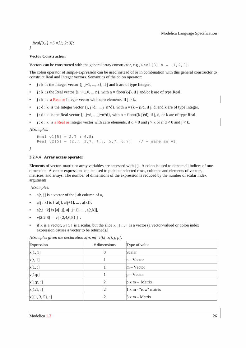
3.2.4.4 Array access operator
Elements of vector, matrix or array variables are accessed with []. A colon is used to denote all indices of onedimension. A vector expression can be used to pick out selected rows, columns and elements of vectors,matrices, and arrays. The number of dimensions of the expression is reduced by the number of scalar indexarguments.
[Examples:
• a[:, j] is a vector of the j-th column of a,
• a[j : k] is {[a[j], a[j+1], ... , a[k]},
• a[:,j : k] is [a[:,j], a[:,j+1], ... , a[:,k]],
• v[2:2:8] = v[ {2,4,6,8} ] .
• if x is a vector, x[1] is a scalar, but the slice x[1:5] is a vector (a vector-valued or colon indexexpression causes a vector to be returned).]
[Examples given the declaration x[n, m], v[k], z[i, j, p]:
Expression # dimensions Type of value
x[1, 1] 0 Scalar
x[:, 1] 1 n – Vector
x[1, :] 1 m – Vector
v[1:p] 1 p – Vector
x[1:p, :] 2 p x m – Matrix
x[1:1, :] 2 1 x m - "row" matrix
x[{1, 3, 5}, :] 2 3 x m – Matrix
Modelica Language Specification
Modelica 1.2 27
x[: , v] 2 n x k – Matrix
z[: , 3, :] 2 i x p – Matrix
x[scalar([1]), :] 1 m – Vector
x[vector([1]), :] 2 1 x m - "row" matrix
]
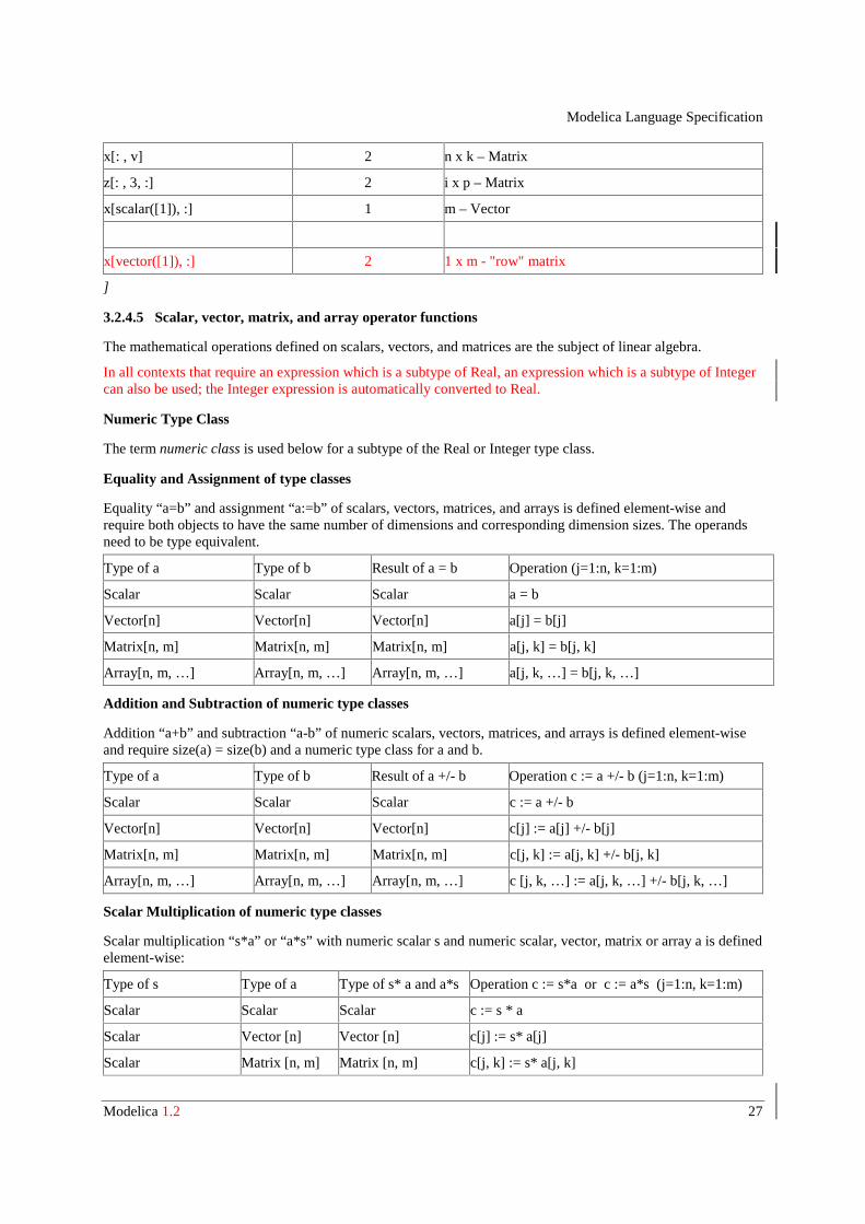
3.2.4.5 Scalar, vector, matrix, and array operator functions
The mathematical operations defined on scalars, vectors, and matrices are the subject of linear algebra.
In all contexts that require an expression which is a subtype of Real, an expression which is a subtype of Integercan also be used; the Integer expression is automatically converted to Real.
Numeric Type Class
The term numeric class is used below for a subtype of the Real or Integer type class.
Equality and Assignment of type classes
Equality “a=b” and assignment “a:=b” of scalars, vectors, matrices, and arrays is defined element-wise andrequire both objects to have the same number of dimensions and corresponding dimension sizes. The operandsneed to be type equivalent.
Type of a Type of b Result of a = b Operation (j=1:n, k=1:m)
Scalar Scalar Scalar a = b
Vector[n] Vector[n] Vector[n] a[j] = b[j]
Matrix[n, m] Matrix[n, m] Matrix[n, m] a[j, k] = b[j, k]
Array[n, m, …] Array[n, m, …] Array[n, m, …] a[j, k, …] = b[j, k, …]
Addition and Subtraction of numeric type classes
Addition “a+b” and subtraction “a-b” of numeric scalars, vectors, matrices, and arrays is defined element-wiseand require size(a) = size(b) and a numeric type class for a and b.
Type of a Type of b Result of a +/- b Operation c := a +/- b (j=1:n, k=1:m)
Scalar Scalar Scalar c := a +/- b
Vector[n] Vector[n] Vector[n] c[j] := a[j] +/- b[j]
Matrix[n, m] Matrix[n, m] Matrix[n, m] c[j, k] := a[j, k] +/- b[j, k]
Array[n, m, …] Array[n, m, …] Array[n, m, …] c [j, k, …] := a[j, k, …] +/- b[j, k, …]
Scalar Multiplication of numeric type classes
Scalar multiplication “s*a” or “a*s” with numeric scalar s and numeric scalar, vector, matrix or array a is definedelement-wise:
Type of s Type of a Type of s* a and a*s Operation c := s*a or c := a*s (j=1:n, k=1:m)
Scalar Scalar Scalar c := s * a
Scalar Vector [n] Vector [n] c[j] := s* a[j]
Scalar Matrix [n, m] Matrix [n, m] c[j, k] := s* a[j, k]
Modelica Language Specification
Modelica 1.2 28
Scalar Array[n, m, ...] Array [n, m, ...] c[j, k, ...] := s*a[j, k, ...]
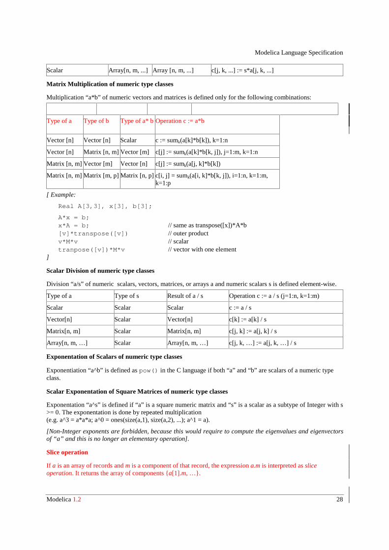
Matrix Multiplication of numeric type classes
Multiplication “a*b” of numeric vectors and matrices is defined only for the following combinations:
Type of a Type of b Type of a* bOperation c := a*b
Vector [n] Vector [n] Scalar c := sumk(a[k]*b[k]), k=1:n
Vector [n] Matrix [n, m] Vector [m] c[j] := sumk(a[k]*b[k, j]), j=1:m, k=1:n
Matrix [n, m] Vector [m] Vector [n] c[j] := sumk(a[j, k]*b[k])
Matrix [n, m] Matrix [m, p] Matrix [n, p] c[i, j] = sumk(a[i, k]*b[k, j]), i=1:n, k=1:m,k=1:p
[ Example:
Real A[3,3], x[3], b[3];
A*x = b; x*A = b; // same as transpose([x])*A*b [v]*transpose([v]) // outer product v*M*v // scalar tranpose([v])*M*v // vector with one element]
Scalar Division of numeric type classes
Division “a/s” of numeric scalars, vectors, matrices, or arrays a and numeric scalars s is defined element-wise.
Type of a Type of s Result of a / s Operation c := a / s (j=1:n, k=1:m)
Scalar Scalar Scalar c := a / s
Vector[n] Scalar Vector[n] c[k] := a[k] / s
Matrix[n, m] Scalar Matrix[n, m] c[j, k] := a[j, k] / s
Array[n, m, …] Scalar Array[n, m, …] c[j, k, …] := a[j, k, …] / s
Exponentation of Scalars of numeric type classes
Exponentiation “a^b” is defined as pow() in the C language if both “a” and “b” are scalars of a numeric typeclass.
Scalar Exponentation of Square Matrices of numeric type classes
Exponentation “a^s” is defined if “a” is a square numeric matrix and “s” is a scalar as a subtype of Integer with s>= 0. The exponentation is done by repeated multiplication (e.g. a^3 = a*a*a; a^0 = ones(size(a,1), size(a,2), ...); a^1 = a).
[Non-Integer exponents are forbidden, because this would require to compute the eigenvalues and eigenvectorsof “a” and this is no longer an elementary operation].
Slice operation
If a is an array of records and m is a component of that record, the expression a.m is interpreted as sliceoperation. It returns the array of components {a[1].m, …}.
Modelica Language Specification
Modelica 1.2 29
If m is also an array component, the slice operation is valid only if size(a[1].m)=size(a[2].m)=… Relationaloperators
Relational operators
Relational operators <, <=, >, >=, ==, <>, are only defined for scalar arguments. The result is Boolean and istrue or false if the relation is fulfilled or not, respectively.
In relations of the form v1 == v2 or v1 <> v2, v1 or v2 shall not be a subtype of Real. [The reason for this rule isthat relations with Real arguments are transformed to state events (see section Events below) and thistransformation becomes unnecessarily complicated for the == and <> relational operators (e.g. two crossingfunctions instead of one crossing function needed, epsilon strategy needed even at event instants). Furthermore,testing on equality of Real variables is questionable on machines where the number length in registers isdifferent to number length in main memory].
Relations of the form “v1 rel_op v2”, with v1 and v2 variables and rel_op a relational operator are calledelementary relations. If either v1 or v2 or both variables are a subtype of Real, the relation is called a Realelementary relation.
Functions
Functions with one scalar return value can be applied to arrays element-wise, e.g. if A is a vector of reals, thensin(A) is a vector where each element is the result of applying the function sin to the corresponding element inA.
Consider the expression f(arg1,...,argn), an application of the function f to the arguments arg1, ..., argnis defined.
For each passed argument, the type of the argument is checked against the type of the corresponding formalparameter of the function.
1. If the types match, nothing is done.
2. If the types do not match, and a type conversion can be applied, it is applied. Continued with step 1.
3. If the types do not match, and no type conversion is applicable, the passed argument type is checked to see ifit is an n-dimensional array of the formal parameter type. If it is not, the function call is invalid. If it is, wecall this a foreach argument.
4. For all foreach arguments, the number and sizes of dimensions must match. If they do not match, thefunction call is invalid.If no foreach arguments exists, the function is applied in the normal fashion, and theresult has the type specified by the function definition.
5. The result of the function call expression is an n-dimensional array with the same dimension sizes as theforeach arguments. Each element ei,..,j is the result of applying f to arguments constructed from the originalarguments in the following way.
• If the argument is not a foreach argument, it is used as-is.
• If the argument is a foreach argument, the element at index [i,...,j] is used.
If more than one argument is an array, all of them have to be the same size, and they are traversed in parallel.
[Examples:
sin({a, b, c}) = {sin(a), sin(b), sin(c)} // argument is a vector sin([a,b,c]) = [sin(a),sin(b),sin(c)] // argument may be a matrix atan({a,b,c},{d,e,f}) = {atan(a,d), atan(b,e), atan(c,f)}
This works even if the function is declared to take an array as one of its arguments. If pval is defined as afunction that takes one argument that is a vector of Reals and returns a Real, then it can be used with an actualargument which is a two-dimensional array (a vector of vectors). The result type in this case will be a vector ofReal.
Modelica Language Specification
Modelica 1.2 30
pval([1,2;3,4]) = [pval([1,2]); pval([3,4])]
sin([1,2;3,4]) = [sin({1,2}); sin({3,4})]
= [sin(1), sin(2); sin(3), sin(4)]
function Add input Real e1, e2; output Real sum1; algorithm sum1 := e1 + e2; end Add;
Add(1, [1, 2, 3]) adds one to each of the elements of the second argument giving the result [2, 3, 4]. However, itis illegal to write 1 + [1, 2, 3], because the rules for the built-in operators are more restrictive.]
Empty Arrays
Arrays may have dimension sizes of 0. E.g. Real x[0]; // an empty vector Real A[0, 3], B[5, 0], C[0, 0]; // empty matrices
• Empty matrices can be constructed with the fill function. E.g. Real A[:,:] = fill(0.0, 0, 1) // a Real 0 x 1 matrix Boolean B[:, :, :] = fill(false, 0, 1, 0) // a Boolean 0 x 1 x 0 matrix
• It is not possible to access an element of an empty matrix, e.g. v[j,k] is wrong if “v=[]” because the assertionfails that the index must be bigger than one.
• Size-requirements of operations, such as +, -, have also to be fulfilled if a dimension is zero. E.g. Real[3,0] A, B; Real[0,0] C; A + B // fine, result is an empty matrix A + C // error, sizes do not agree
• Multiplication of two empty matrices results in a zero matrix if the result matrix has no zero dimensionsizes, i.e., Real[0,m]*Real[m,n] = Real[0,n] (empty matrix) Real[m,n]*Real[n,0] = Real[m,0] (empty matrix) Real[m,0]*Real[0,n] = zeros(m,n) (non-empty matrix, with zero elements).
[Example:
Real u[p], x[n], y[q], A[n,n], B[n,p], C[q,n], D[q,p];
der(x) = A*x + B*u y = C*x + D*u
Assume n=0, p>0, q>0: Results in "y = D*u"
]
3.2.5 Final element modification
An element defined as final in an element modification cannot be modified by a modification or by aredeclaration. All elements of a final element are also final. [Setting the value of a parameter in an experimentenvironment is conceptually treated as a modification. This implies that a final modification equation of aparameter cannot be changed in a simulation environment].
[Examples:
type Angle = Real(final quantity=”Angle”, final unit =”rad”, displayUnit=”deg”);Angle a1(unit=”deg”); // error, since unit declared as final!
Modelica Language Specification
Modelica 1.2 31
Angle a2(displayUnit=”rad”); // fine
model TransferFunction parameter Real b[:] = {1} ”numerator coefficient vector”; parameter Real a[:] = {1,1} ”denominator coefficient vector”; ...end TransferFunction;
model PI ”PI controller”; parameter Real k=1 ”gain”; parameter Real T=1 ”time constant”; TransferFunction tf( final b={T,1}, final a={T,0});end PI;
model Test PI c1(k=2, T=3); // fine PI c2(b={1}); // error, b is declared as finalend Test;
]
Note: In the previous versions of Modelica (Modelica 1.0 and 1.1), the final keyword had three differentmeanings depending on the situation where it was used. To simplify the semantics, in Modelica 1.2, final is onlyused in modifications to prevent further modifications and redeclarations. As a consequence, components have tobe explicitly defined as replaceable, if they shall be redeclared (previously, this was the default and final wasused to prevent redeclarations).
3.2.6 Short class definition
A class definition of the form
class IDENT 1 = IDENT 2 class_modification ;
is identical to the longer form
class IDENT 1
extends IDENT 2 class_modification ;end IDENT1;
A short class definition of the form
type TN = T[N] (optional modifier) ;
where N represents arbitrary array dimensions, conceptually yields an array class
array TN T[n] _ (optional modifiers);end TN;
Such an array class has exactly one anonymous component (_). When a component of such an array class type isinstantiated, the resulting instantiated component type is an array type with the same dimensions as _ and withthe optional modifier applied.
[Example:
type Force = Real[3](unit={ "Nm ", "Nm", "Nm "});Force f1;Real f2[3](unit={ "Nm", "Nm", "Nm "});
the types of f1 and f2 are identical.]
Modelica Language Specification
Modelica 1.2 32
3.2.7 Local class definition
The local class is instantiated with the partially instantiated parent of the local class. The environment is themodification of any parent class element modification with the same name as the local class, or an emptyenvironment.
The instantiated local class becomes an element of the instantiated parent class.
[The following example demonstrates parameterization of a local class:
class C1 class Voltage = Real(unit="V"); Voltage v1, v2;end C1;class C2 extends C1(Voltage(unit="kV"));end C2;
Instantiation of class C2 yields a local instance of class Voltage with unit "kV". The variables v1 and v2 thushave unit "kV".]
3.2.8 Extends clause
The name of the base class is looked up in the partially instantiated parent of the extends clause. The found baseclass is instantiated with a new environment and the partially instantiated parent of the extends clause. The newenvironment is the result of merging
• arguments of all parent environments that match names in the instantiated base class
• the modification of a parent element-modification with the same name as the base class
• the optional class modification of the extends clause
in that order.
[Examples of the three rules are given in the following example:
class A parameter Real a, b; end A;class B extends A(b=3); // Rule #3end B;class C extends B(a=1, A(b=2)); // Rules #1 and #2end C;
]
The elements of the instantiated base class become elements of the instantiated parent class.
[From the example above we get the following instantiated class:
class Cinstance parameter Real a=1; parameter Real b=2;end Cinstance;
The ordering of the merging rules ensures that, given classes A and B defined above,
class C2 B bcomp(b=1, A(b=2));end C2;
yields an instance with bcomp.b=1, which overrides b=2.]
The declaration elements of the instantiated base class shall either
Modelica Language Specification
Modelica 1.2 33
• Not already exist in the partially instantiated parent class [i.e., have different names] .
• Be identical to any element of the instantiated parent class with the same name and the same level ofprotection (public or protected). In this case, the element of the instantiated base class is ignored.
Otherwise the model is incorrect.
[The second rule says that if an element is inherited multiple times, the first inherited element overrides laterinherited elements:
class A parameter Real a, b; end A;
class B extends A(a=1); extends A(b=2);end B;
Class B is well-formed and yields an instantiated object with elements a and b inherited from the first extendsclause:
class Binstance parameter Real a=1; parameter Real b;end Binstance;
]
Equations of the instantiated base class that are syntactically equivalent to equations in the instantiated parentclass are discarded. [Note: equations that are mathematically equivalent but not syntactically equivalent are notdiscarded, hence yield an overdetermined system of equations.]
3.2.9 Redeclaration
A redeclare construct replaces the declaration of an extends clause, local class or component in the modifiedelement with another declaration. The type specified in the redeclaration shall be a subtype of the type in theoriginal declaration.
The element modifications of the redeclaration and the original declaration are merged in the usual way.
[Example:
class A parameter Real x; end A;class B parameter Real x=3.14, y; // B is a subtype of Aend B;class C replaceable A a(x=1);end C;class D extends C(redeclare B a(y=2));end D;
which effectively yields a class D2 with the contents
class D2 B a(x=1, y=2);end D2;
]
The following additional constraints apply to redeclarations:
Modelica Language Specification
Modelica 1.2 34
• only classes and components declared as replaceable can be redeclared with a new type and to allowfurther redeclarations one must use “redeclare replaceable”
• a replaceable class used in an extends clause shall only contain public components [otherwise, itcannot be guaranteed that a redeclaration keeps the protected variables of the replaceable defaultclass]
• an element declared as constant cannot be redeclared
• an element declared as parameter can only be redeclared with parameter or constant
• an element declared as discrete can only be redeclared with discrete, parameter or constant
• a function can only be redeclared as function
• an element declared as flow can only be redeclared with flow
• an element declared as not flow can only be redeclared without flow
Modelica does not allow a protected element to be redeclared as public, or a public element to be redeclared asprotected.
Array dimensions may be redeclared.
3.3 Equations
3.3.1 Equation clause
The instantiated equation is identical to the non-instantiated equation.
Names in an equation shall be found by looking up in the partially instantiated parent of the equation.
Equation equality = shall not be used in an algorithm clause. The assignment operator := shall not be used in anequation clause.
3.3.2 If clause
If clauses in equation sections which do not have exclusively parameter expressions as switching conditionsshall have an else clause and each branch shall have the same number of equations. [If this condition is violated,the single assignment rule would not hold, because the number of equations may change during simulationalthough the number of unknowns remains the same].
3.3.3 For clause
The expression of a for clause shall be a vector expression. It is evaluated once for each for clause. In anequation section, the expression of a for clause shall be a parameter expression.
[Example:
for i in 1:10 loop // i takes the values 1,2,3,...,10 for r in 1.0 : 1.5 : 5.5 loop // r takes the values 1.0, 2.5, 4.0, 5.5 for i in {1,3,6,7} loop // i takes the values 1, 3, 6, 7
]
3.3.4 When clause
The expression of a when clause shall be a discrete Boolean scalar or vector expression. The equations within awhen clause are activated when the scalar or any one of the elements of the vector expression becomes true. Awhen clause shall not be used within a function class.
[Example:
Modelica Language Specification
Modelica 1.2 35
Equations are activated when x becomes > 2:
when x > 2 then y1 = 2*x + y2; y2 = sin(x); end when;
Equations are activated when either x becomes > 2 or sample(0,2) becomes true or x becomes less than 5:
when {x > 2, sample(0,2), x < 5} then y1 = 2*x + y2; y2 = sin(x); end when;
The equations in a when clause are sorted independently from each other with all other equations.]
A when clause
when {condition1, condition2, ..., conditionN} then ... end when;
is equivalent to the following special if-clause, where Boolean b[N]; is necessary because we can only applyedge to variables
b:={condition1, condition2, ..., conditionN};
if edge(b[1]) or edge(b[2]) or ... edge(b[N]) then ... end if;
with “edge(A)= A and not pre(A)” and the additional guarantee, that the equations within this specialif clause are only evaluated at event instants.
When clauses cannot be nested.
[Example:
The following when clause is invalid:
when x > 2 then when y1 > 3 then y2 = sin(x); end when; end when;
]
3.3.5 Assert
The expression of an assert clause shall evaluate to true. [The intent is to perform a test of model validity and toreport the failed assertion to the user if the expression evaluates to false. The means of reporting a failedassertion are dependent on the simulation environment. The intention is that the current evaluation of the modelshould stop if when an assert with a false condition is encountered, but the tool should continue the currentanalysis (e.g. by using a shorter stepsize).]
3.3.6 Connections
Connections between objects are introduced by the connect statement in the equation part of a class. Theconnect construct takes two references to connectors, each of which is either an element of the same class as theconnect statement (an outer connector) or an element of one of its components (an inner connector). The twomain tasks are to:
• Build connection sets from connect statements.
Modelica Language Specification
Modelica 1.2 36
• Generate equations for the complete model.
Definitions:
Connection sets
A connection set is a set of variables connected by means of connect clause. A connection set shallcontain either only flow variables or only non-flow variables.
Inner and outer connectors
In a class M, each connector element of that class is called an outer connector with respect to M. Eachconnector element of some element of M is called an inner connector with respect to M.
3.3.6.1 Generation of connection equations
For every use of the connect statementconnect(a, b);
the primitive components of a and b form a connection set. If any of them already occur in a connection setfrom previous connects in the same class or nested components, these sets are merged to form one connectionset. Composite connector types are broken down into primitive components. Each connection set is used togenerate equations for across and through (zero-sum) variables of the form
a1 = a2 = ... = an;z1 + z2 + (-z3) + ... + zn = 0;
In order to generate equations for through variables [using the flow prefix], the sign used for the connectorvariable zi above is +1 for inner connectors and -1 for outer connectors [z3 in the example above].
For each unconnected through (zero-sum) variable the following equation is implicitly generated:
z = 0;
3.3.6.2 Restrictions
A component of an inner connector declared with the input type prefix shall not occur in more than one connectstatement in that scope. A component of an outer connector declared with the output type prefix shall not occurin more than one connect statement in that scope. Two components declared with the input type prefix shall notbe connected in the same scope. Two components declared with the output type prefix shall not be connected inthe same scope.
Subscripts in a connector reference shall be constant expressions.
If the array sizes do not match, the original variables are filled with one-sized dimensions from the left until thenumber of dimensions match before the connection set equations are generated.
Constants or parameters in connected components yield the appropriate assert statements; connections are notgenerated.
3.4 Functions
There are two forms of function application, see section 2.2.7. In the first form,
f(3.5, 5.76)
the arguments are associated with the [formal] parameters according to their position in the argument list. Thusargument i is passed to parameter i, where the order of the parameters is given by the order of the componentdeclarations in the function definition. The first input component is parameter number 1, the second inputcomponent is parameter number 2, and so on. When a function is called in this way, the number of argumentsand parameters must be the same.
In the second form of function application,
g(x=3.5, y=5.76)
Modelica Language Specification
Modelica 1.2 37
the parameters are explicitly associated with the arguments by means of equations in the argument list.Parameters which have default values need not be specified in the argument list.
The type of each argument must agree with the type of the corresponding parameter, except where the standardtype coercions can be used to make the types agree. (See also section 3.2.2.5 on applying scalar functions toarrays.)
[Example. Suppose a function f is defined as follows:
function f input Real x; input Real y; input Real z = 10.0; output Real r; ...end f;
Then the following two applications are equivalent:
f(1.0, 2.0, 10.0) f(y = 2.0, x = 1.0)
]
A function may have more than one output component, corresponding to multiple return values. When a functionhas a single return value, a function application is an expression whose value and type are given by the value andtype of the output component.
The only way to call a function having more than one output component is to make the function call the RHS ofan equation or assignment. In these cases, the LHS of of the equation or assignment must be a list of componentreferences within parentheses. The component references are associated with the output components accordingto their position in the list. Thus output component i is set equal to, or assigned to, component reference i in thelist, where the order of the output components is given by the order of the component declarations in the functiondefinition.
The number of component references in the list must agree with the number of output components.
The type of each output parameter must agree with the type of the corresponding component references in thelist on the LHS.
[Example. Suppose a function f is defined as follows:
function f input Real x; input Real y; output Real r1; output Real r2; output Real r3; ...end f;
Then the following equation and assignment show the two possible ways of calling f:
(x, y, z) = f(1.0, 2.0); (x, y, z) := f(1.0, 2.0);
]
The only permissible use of an expression in the form of a list of expressions in parentheses, is when it is used asthe LHS of an equation or assignment where the RHS is an application of a function with more than one outputcomponent. In this case, the expressions in the list shall be component references.
[Example. The following are illegal:
(x+1, 3.0, z/y) = f(1.0, 2.0); // Not a list of component references.
Modelica Language Specification
Modelica 1.2 38
(x, y, z) + (u, v, w) // Not LHS of suitable eqn/assignment.
]
3.5 Code Optimizations
A tool is free to solve equations, reorder expressions and to not evaluate expressions if their value does notinfluence the result. If-statements and if-expressions guarantee that their clauses are only evaluated if theappropriate condition is true.
[Example. If one wants to guard an expression against evaluation it should be guarded by an if
Boolean v[n]; Boolean b; Integer I;equation x=v[I] and (I>=1 and I<=n); // Invalid x=if (I>=1 and I<=n) then v[I] else false; // Correct
]
3.6 Events and Synchronization
The integration is halted and an event occurs whenever a Real elementary relation, e.g. “x > 2”, changes itsvalue. The value of a relation can only be changed at event instants [in other words, Real elementary relationsinduce state or time events]. The relation which triggered an event changes its value when evaluated literallybefore the model is processed at the event instant [in other words, a root finding mechanism is needed whichdetermines a small time interval in which the relation changes its value; the event occurs at the right side of thisinterval]. At an event instant, a relation is taken literally. During continuous integration a Real elementaryrelation has the constant value of the relation from the last event instant.
[Example:
y = if u > uMax then uMax else if u < uMin then uMin else u;
During continuous integration always the same if branch is evaluated. The integration is halted whenever u-uMax or u-uMin crosses zero. At the event instant, the correct if-branch is selected and the integration isrestarted.
Numerical integration methods of order n (n>=1) require continuous model equations which are differentiableupto order n. This requirement can be fulfilled if Real elementary relations are not treated literally but asdefined above, because discontinuous changes can only occur at event instants and no longer during continuousintegration.]
[It is a quality of implementation issue that the following special relations
time >= discrete expression time < discrete expression
trigger a time event at “time = discrete expression”, i.e., the event instant is known in advance and no iterationis needed to find the exact event instant.]
Relations are taken literally also during continuous integration, if the relation or the expression in which the
Modelica Language Specification
Modelica 1.2 39
relation is present, are the argument of the noEvent(..) function. The noEvent feature is propagated to allsubrelations in the scope of the noEvent function.
[Example:
y = noEvent( if u > uMax then uMax else if u < uMin then uMin else u);
The if-expression is taken literally without inducing state events.
The noEvent function is useful, if e.g. the modeller can guarantee that the used if-clauses fulfill at least thecontinuity requirement of integrators. In this case the simulation speed is improved, since no state eventiterations occur during integration. Furthermore, the noEvent function is used to guard agains “outsidedomain” errors, e.g. y = if noEvent(x >= 0) then sqrt(x) else 0.]
All equations and assignment statements within when clauses and all assignment statements within functionclasses are implicitly treated with the noEvent function, i.e., relations within the scope of these operators neverinduce state or time events. [Using state events in when-clauses is unnecessary because the body of a whenclause is not evaluated during continuous integration.]
[Example:
Limit1 = noEvent(x1 > 1); Limit2 = x2 > 10; Limit = Limit1 or Limit2; when Limit then // error, Limit is no discrete expression Close = true; end when;
This is an error, because Limit1 may change during continuous integeration, i.e., it is not a discrete-timevariable and therefore the when condition Limit is also no discrete-time variable (when conditions need to bediscrete expressions in order to guarantee that when-equations are never evaluated during continuous
integration).
Modelica is based on the synchronous data flow principle which is defined in the following way:
1. All variables keep their actual values until these values are explicitly changed. Variable values can beaccessed at any time instant during continuous integration and at event instants.
2. At every time instant, during continuous integration and at event instants, the active equations expressrelations between variables which have to be fulfilled concurrently (equations are not active if thecorresponding if-branch, when-clause or block in which the equation is present is not active).
3. Computation and communication at an event instant does not take time. [If computation or communicationtime has to be simulated, this property has to be explicitly modeled].
4. The total number of equations is identical to the total number of unknown variables (= single assignmentrule).
[These rules guarantee that variables are always defined by a unique set of equations. It is not possible that avariable is e.g. defined by two equations, which would give rise to conflicts or non-deterministic behaviour.Furthermore, the continuous and the discrete parts of a model are always automatically “synchronized”.Example:
when condition1 then close = true; end when;
when condition2 then close = false; end when;
This is not a valid model because rule 4 is violated since there are two equations for the single unknown variableclose. If this would be a valid model, a conflict occurs when both conditions become true at the same timeinstant, since no priorities between the two equations are assigned. To become valid, the model has to bechanged to:
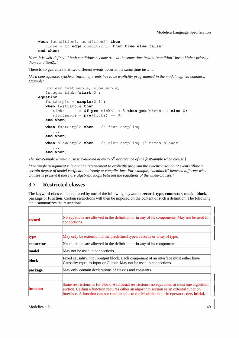
Modelica Language Specification
Modelica 1.2 40
when {condition1, condition2} then close = if edge(condition1) then true else false; end when;
Here, it is well-defined if both conditions become true at the same time instant (condition1 has a higher prioritythan condition2).]
There is no guarantee that two different events occur at the same time instant.
[As a consequence, synchronization of events has to be explicitly programmed in the model, e.g. via counters.Example:
Boolean fastSample, slowSample; Integer ticks(start=0); equation fastSample = sample(0,1); when fastSample then ticks = if pre(ticks) < 5 then pre(ticks)+1 else 0; slowSample = pre(ticks) == 0; end when;
when fastSample then // fast sampling ... end when;
when slowSample then // slow sampling (5-times slower) ... end when;
The slowSample when-clause is evaluated at every 5th occurrence of the fastSample when clause.]
[The single assignment rule and the requirement to explicitly program the synchronization of events allow acertain degree of model verification already at compile time. For example, “deadlock” between different when-clauses is present if there are algebraic loops between the equations of the when-clauses.]
3.7 Restricted classes
The keyword class can be replaced by one of the following keywords: record, type, connector, model, block,package or function. Certain restrictions will then be imposed on the content of such a definition. The followingtable summarizes the restrictions.
recordNo equations are allowed in the definition or in any of its components. May not be used inconnections.
type May only be extension to the predefined types, records or array of type.
connector No equations are allowed in the definition or in any of its components.
model May not be used in connections.
blockFixed causality, input-output block. Each component of an interface must either haveCausality equal to Input or Output. May not be used in connections.
package May only contain declarations of classes and constants.
functionSame restrictions as for block. Additional restrictions: no equations, at most one algorithmsection. Calling a function requires either an algorithm section or an external functioninterface. A function can not contain calls to the Modelica built-in operators der, initial,
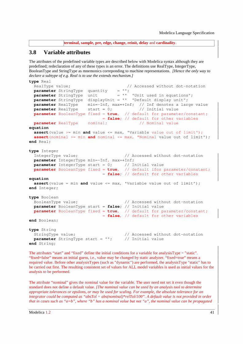
Modelica Language Specification
Modelica 1.2 41
terminal, sample, pre, edge, change, reinit, delay and cardinality.
3.8 Variable attributes
The attributes of the predefined variable types are described below with Modelica syntax although they arepredefined; redeclaration of any of these types is an error. The definitions use RealType, IntegerType,BooleanType and StringType as mnemonics correponding to machine representations. [Hence the only way todeclare a subtype of e.g. Real is to use the extends mechanism.]
type Real RealType value; // Accessed without dot-notation parameter StringType quantity = ""; parameter StringType unit = "" "Unit used in equations"; parameter StringType displayUnit = "" "Default display unit"; parameter RealType min=-Inf, max=+Inf; // Inf denotes a large value parameter RealType start = 0; // Initial value parameter BooleanType fixed = true, // default for parameter/constant; = false; // default for other variables parameter RealType nominal; // Nominal valueequation assert(value >= min and value <= max, "Variable value out of limit"); assert(nominal >= min and nominal <= max, "Nominal value out of limit");end Real;
type Integer IntegerType value; // Accessed without dot-notation parameter IntegerType min=-Inf, max=+Inf; parameter IntegerType start = 0; // Initial value parameter BooleanType fixed = true, // default ifor parameter/constant; = false; // default for other variablesequation assert(value = min and value <= max, "Variable value out of limit");end Integer;
type Boolean BooleanType value; // Accessed without dot-notation parameter BooleanType start = false; // Initial value parameter BooleanType fixed = true, // default for parameter/constant; = false, // default for other variablesend Boolean;
type String StringType value; // Accessed without dot-notation parameter StringType start = ""; // Initial valueend String;
The attributes “start” and “fixed” define the initial conditions for a variable for analysisType = "static".“fixed=false” means an initial guess, i.e., value may be changed by static analyzer. “fixed=true” means arequired value. Before other analysisTypes (such as "dynamic") are performed, the analysisType "static" has tobe carried out first. The resulting consistent set of values for ALL model variables is used as initial values for theanalysis to be performed.
The attribute “nominal” gives the nominal value for the variable. The user need not set it even though thestandard does not define a default value. [The nominal value can be used by an analysis tool to determineappropriate tolerances or epsilons, or may be used for scaling. For example, the absolute tolerance for anintegrator could be computed as “absTol = abs(nominal)*relTol/100”. A default value is not provided in orderthat in cases such as “a=b”, where “b” has a nominal value but not “a”, the nominal value can be propagated
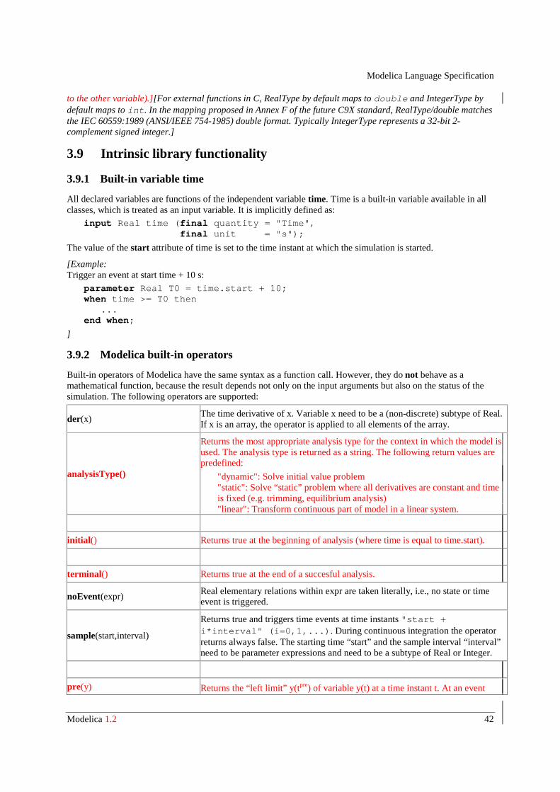
Modelica Language Specification
Modelica 1.2 42
to the other variable).][For external functions in C, RealType by default maps to double and IntegerType bydefault maps to int. In the mapping proposed in Annex F of the future C9X standard, RealType/double matchesthe IEC 60559:1989 (ANSI/IEEE 754-1985) double format. Typically IntegerType represents a 32-bit 2-complement signed integer.]
3.9 Intrinsic library functionality
3.9.1 Built-in variable time
All declared variables are functions of the independent variable time. Time is a built-in variable available in allclasses, which is treated as an input variable. It is implicitly defined as:
input Real time (final quantity = "Time", final unit = "s");
The value of the start attribute of time is set to the time instant at which the simulation is started.
[Example:Trigger an event at start time + 10 s:
parameter Real T0 = time.start + 10;when time >= T0 then ...end when;
]
3.9.2 Modelica built-in operators
Built-in operators of Modelica have the same syntax as a function call. However, they do not behave as amathematical function, because the result depends not only on the input arguments but also on the status of thesimulation. The following operators are supported:
der(x)The time derivative of x. Variable x need to be a (non-discrete) subtype of Real.If x is an array, the operator is applied to all elements of the array.
analysisType()
Returns the most appropriate analysis type for the context in which the model isused. The analysis type is returned as a string. The following return values arepredefined:
"dynamic": Solve initial value problem"static": Solve “static” problem where all derivatives are constant and timeis fixed (e.g. trimming, equilibrium analysis)"linear": Transform continuous part of model in a linear system.
initial() Returns true at the beginning of analysis (where time is equal to time.start).
terminal() Returns true at the end of a succesful analysis.
noEvent(expr)Real elementary relations within expr are taken literally, i.e., no state or timeevent is triggered.
sample(start,interval)
Returns true and triggers time events at time instants "start +i*interval" (i=0,1,...). During continuous integration the operatorreturns always false. The starting time “start” and the sample interval “interval”need to be parameter expressions and need to be a subtype of Real or Integer.
pre(y) Returns the “left limit” y(tpre) of variable y(t) at a time instant t. At an event
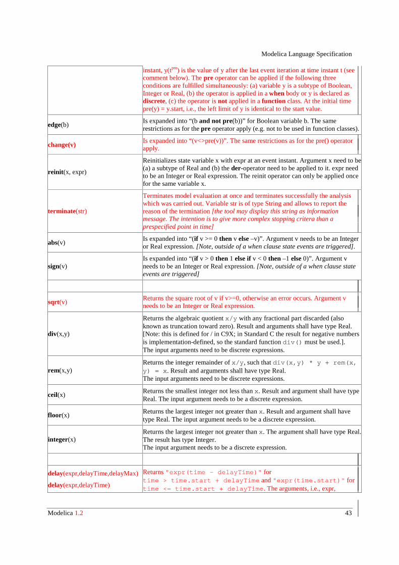
Modelica Language Specification
Modelica 1.2 43
instant, y(tpre) is the value of y after the last event iteration at time instant t (seecomment below). The pre operator can be applied if the following threeconditions are fulfilled simultaneously: (a) variable y is a subtype of Boolean,Integer or Real, (b) the operator is applied in a when body or y is declared asdiscrete, (c) the operator is not applied in a function class. At the initial timepre(y) = y.start, i.e., the left limit of y is identical to the start value.
edge(b)Is expanded into “(b and not pre(b))” for Boolean variable b. The samerestrictions as for the pre operator apply (e.g. not to be used in function classes).
change(v)Is expanded into “(v<>pre(v))”. The same restrictions as for the pre() operatorapply.
reinit(x, expr)
Reinitializes state variable x with expr at an event instant. Argument x need to be(a) a subtype of Real and (b) the der-operator need to be applied to it. expr needto be an Integer or Real expression. The reinit operator can only be applied oncefor the same variable x.
terminate(str)
Terminates model evaluation at once and terminates successfully the analysiswhich was carried out. Variable str is of type String and allows to report thereason of the termination [the tool may display this string as informationmessage. The intention is to give more complex stopping critera than aprespecified point in time]
abs(v)Is expanded into “(if v >= 0 then v else –v)”. Argument v needs to be an Integeror Real expression. [Note, outside of a when clause state events are triggered].
sign(v)Is expanded into “(if v > 0 then 1 else if v < 0 then –1 else 0)”. Argument vneeds to be an Integer or Real expression. [Note, outside of a when clause stateevents are triggered]
sqrt(v)Returns the square root of v if v>=0, otherwise an error occurs. Argument vneeds to be an Integer or Real expression.
div(x,y)
Returns the algebraic quotient x/y with any fractional part discarded (alsoknown as truncation toward zero). Result and arguments shall have type Real.[Note: this is defined for / in C9X; in Standard C the result for negative numbersis implementation-defined, so the standard function div() must be used.].The input arguments need to be discrete expressions.
rem(x,y)Returns the integer remainder of x/y, such that div(x,y) * y + rem(x,y) = x. Result and arguments shall have type Real.The input arguments need to be discrete expressions.
ceil(x)Returns the smallest integer not less than x. Result and argument shall have typeReal. The input argument needs to be a discrete expression.
floor(x)Returns the largest integer not greater than x. Result and argument shall havetype Real. The input argument needs to be a discrete expression.
integer(x)Returns the largest integer not greater than x. The argument shall have type Real.The result has type Integer.The input argument needs to be a discrete expression.
delay(expr,delayTime,delayMax)
delay(expr,delayTime)
Returns "expr(time – delayTime)" for time > time.start + delayTime and "expr(time.start)" fortime <= time.start + delayTime . The arguments, i.e., expr,
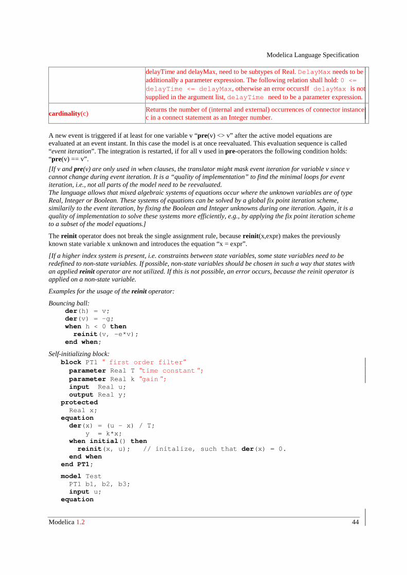
Modelica Language Specification
Modelica 1.2 44
delayTime and delayMax, need to be subtypes of Real. DelayMax needs to beadditionally a parameter expression. The following relation shall hold: 0 <=delayTime <= delayMax, otherwise an error occursIf delayMax is notsupplied in the argument list, delayTime need to be a parameter expression.
cardinality(c)Returns the number of (internal and external) occurrences of connector instancec in a connect statement as an Integer number.
A new event is triggered if at least for one variable v “pre(v) <> v” after the active model equations areevaluated at an event instant. In this case the model is at once reevaluated. This evaluation sequence is called“event iteration”. The integration is restarted, if for all v used in pre-operators the following condition holds:“pre(v) == v”.
[If v and pre(v) are only used in when clauses, the translator might mask event iteration for variable v since vcannot change during event iteration. It is a “quality of implementation” to find the minimal loops for eventiteration, i.e., not all parts of the model need to be reevaluated.The language allows that mixed algebraic systems of equations occur where the unknown variables are of typeReal, Integer or Boolean. These systems of equations can be solved by a global fix point iteration scheme,similarily to the event iteration, by fixing the Boolean and Integer unknowns during one iteration. Again, it is aquality of implementation to solve these systems more efficiently, e.g., by applying the fix point iteration schemeto a subset of the model equations.]
The reinit operator does not break the single assignment rule, because reinit(x,expr) makes the previouslyknown state variable x unknown and introduces the equation “x = expr”.
[If a higher index system is present, i.e. constraints between state variables, some state variables need to beredefined to non-state variables. If possible, non-state variables should be chosen in such a way that states withan applied reinit operator are not utilized. If this is not possible, an error occurs, because the reinit operator isapplied on a non-state variable.
Examples for the usage of the reinit operator:
Bouncing ball: der(h) = v; der(v) = -g; when h < 0 then reinit(v, -e*v); end when;
Self-initializing block: block PT1 " first order filter" parameter Real T "time constant "; parameter Real k "gain "; input Real u; output Real y; protected Real x; equation der(x) = (u – x) / T; y = k*x; when initial() then reinit(x, u); // initalize, such that der(x) = 0. end when end PT1;
model Test PT1 b1, b2, b3; input u; equation
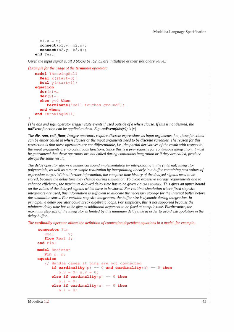
Modelica Language Specification
Modelica 1.2 45
b1.u = u; connect(b1.y, b2.u); connect(b2.y, b3.u); end Test;
Given the input signal u, all 3 blocks b1, b2, b3 are initialized at their stationary value.]
[Example for the usage of the terminate operator:
model ThrowingBall Real x(start=0); Real y(start=1); equation der(x)=… der(y)=… when y<0 then terminate(”ball touches ground”); end when; end ThrowingBall;]
[The abs and sign operator trigger state events if used outside of a when clause. If this is not desired, thenoEvent function can be applied to them. E.g. noEvent(abs(v)) is |v|
The div, rem, ceil, floor, integer operators require discrete expressions as input arguments, i.e., these functionscan be either called in when clauses or the input arguments need to be discrete variables. The reason for thisrestriction is that these operators are not differentiable, i.e., the partial derivatives of the result with respect tothe input arguments are no continuous functions. Since this is a pre-requisite for continuous integration, it mustbe guaranteed that these operators are not called during continuous integration or if they are called, producealways the same result.
The delay operator allows a numerical sound implementation by interpolating in the (internal) integratorpolynomials, as well as a more simple realization by interpolating linearly in a buffer containing past values ofexpression expr. Without further information, the complete time history of the delayed signals need to bestored, because the delay time may change during simulation. To avoid excessive storage requirements and toenhance efficiency, the maximum allowed delay time has to be given via delayMax. This gives an upper boundon the values of the delayed signals which have to be stored. For realtime simulation where fixed step sizeintegrators are used, this information is sufficient to allocate the necessary storage for the internal buffer beforethe simulation starts. For variable step size integrators, the buffer size is dynamic during integration. Inprincipal, a delay operator could break algebraic loops. For simplicity, this is not supported because theminimum delay time has to be give as additional argument to be fixed at compile time. Furthermore, themaximum step size of the integrator is limited by this minimum delay time in order to avoid extrapolation in thedelay buffer.
The cardinality operator allows the definition of connection dependent equations in a model, for example:
connector Pin Real v; flow Real i; end Pin;
model Resistor Pin p, n; equation // Handle cases if pins are not connected if cardinality(p) == 0 and cardinality(n) == 0 then p.v = 0; n.v = 0; else if cardinality(p) == 0 then p.i = 0; else if cardinality(n) == 0 then n.i = 0;

Modelica Language Specification
Modelica 1.2 46
end if
// Equations of resistor ... end Resistor;
]
Modelica Language Specification
Modelica 1.2 47
4 Mathematical description of HybridDAEs
In this section, the mapping of a Modelica model into an appropriate mathematical description form is discussed.
The result of the modeling process is a set of ordinary differential equations, often accompanied with algebraicconstraint equations, thus forming a set of Differential and Algebraic Equations (DAE). The initial values of thestate variables need to be specified, implying that the DAE is mathematically formulated as a so-called InitialValue Problem. This DAE is used for simulation or other analysis activities. DAEs may have discontinuities orthe structure of a DAE may change at certain points in time. Such types of DAEs are called hybrid DAEs. Eventsare used to stop continuous integration at discontinuities of a hybrid DAE. After applying the discontinuouschange, the integration is restarted. A hybrid DAE is mathematically described by a set of equations of the form
(1a) Residue Equations: 0 = f(dx/dt, x, y, t, m), df/[dx/dt;y] is regular (1b) Monitor Functions: z:= g(dx/dt, x, y, t, m) (1c) Update Equations : 0 = h(dx/dt, xknown, xreinit, y, t, m, pre(m))
Additionally, every equation is a function of the parameters p and of the input functions u(t). This dependency isnot explicitly shown in (1) for clarity of the equations. The variables have the following meaning:
t time, the independent (real) variable.
x(t)(Real) variables appearing differentiated (xknown is the part of x which is always known; xreinit is the other part ofx which is reinitialized at an event instant).
y(t) (Real) algebraic variables.
u(t) known (Real) functions of time.
mdiscrete variables of type Real, Boolean or Integer defining the current mode.pre(m) are the values of m immediatly before the current event occured.
p parameters, i.e., variables without any time-dependency.
The residue equations (1a) are used for continuous integration. During integration, the discrete variables m arenot changed. The monitor functions (1b) are also evaluated during continuous integration. If one of the signals zcrosses zero, the integration is halted and an event occurs. The special case of a time event, "z = t - te", is alsoincluded. For efficiency reasons, time events are usually treated in a special way, since the time instant of suchan event is known in advance. At every event instant, the update functions (1c) are used to determine new valuesof the discrete variables and of new initial values for the states x. The change of discrete variables maycharacterize a new structure of a DAE where elements of the state vector x are disabled. In other words, thenumber of state variables, algebraic variables and residue equations of a DAE may change at event instants bydisabling the appropriate part of the DAE. For clarity of the equations, this is not explicitly shown by anadditional index in (1).
At an event instant, including the initial event, the model equations are reinitialized according to the followingiteration procedure: loop solve 0 = f(dx/dt, xknown, xreinit, y, t, m) 0 = h(dx/dt, xknown, xreinit, y, t, m, pre(m)) for dx/dt, xreinit, y, m, where xknown, t, pre(m) are fixed
Modelica Language Specification
Modelica 1.2 48
if m == pre(m) then break pre(m) := m end loop
At every iteration a set of mixed Real, Boolean, Integer equations (1a),(1c) has to be solved for the indicatedvariables. In order that this is possible, at least the Jacobian of (1a) needs to be regular, as it was stated in (1a).This set of equations can e.g. be solved by a global fixed point iteration scheme which can be combined with theevent iteration:
loop solve “ 0 = f(d x/dt, xknown, xreinit, y, t, m)” for d x/dt, y, where xknown, xreinit, t, m are fixed solve “ 0 = h(d x/dt, xknown, xreinit, y, t, m, pre( m))” for xreinit, m where d x/dt, y, xknown, t, pre( m) are fixed if m == pre( m) then break pre(m) := m end loop
The hybrid DAE (1) is not the most general one, but it has a clearly defined view and structure. Especially, (1a)can be transformed into state space form, at least numerically, since the Jacobian is required to be regular.Generalizations are possible in the direction of higher index DAEs where the Jacobian of (1a) is singular. Thisleads to additional difficulties during integration and especially for event restart because the non-linear equationcannot be solved due to the singular Jacobian. Other generalizations concern the determination of the initialconfiguration by allowing the specification of any variable at the initial time and by calculating the remainingones. A third generalization may use other algorithms to determine a consistent configuration after an eventoccurred, e.g., by solving a complementary problem, see (Pfeiffer and Glocker 1996) for details. For a certainclass of higher index DAE systems, algorithms are available to automatically differentiate selected equations of(1a), choose appropriate variables to be no longer states (= dummy derivative method) and transform to a DAE(1) with a regular Jacobian.
The Modelica language allows a direct and convenient specification of physical systems. A Modelica translatormaps a Modelica model into a hybrid DAE (1), or in one of its generalizations if these are available. Themapping into (1) is straightforward by expanding all class definitions (flattening the inheritance tree) and addingthe equations and assignment statements of the expanded classes for every instance of the model to (1). Theresulting hybrid DAE usually contains a huge number of sparse equations. Therefore, direct simulation of ahybrid DAE (1) which was generated by a Modelica translator requires sparse matrix methods.
There are several simulation environments available, such as Allan, Dymola, gPROMS, Ida (NMF) or Omola,which preprocess (1) symbolically to arrive at a form which can be evaluated more efficiently by numericalalgorithms. Especially, efficient graph-theoretical algorithms are available to transform (1) automatically into thefollowing form which is called sorted hybrid DAE: (2a) Residue Equations: 0 = fr(d xi/dt, yi, x,t, m), (2b) Exp. dx-Functions: d xe/dt := fx(d xi/dt, yi, x,t, m) (2c) Exp. y-Functions : ye := fy(d xi/dt, yi, x,t, m) (2d) Monitor Functions: z := g(d xi/dt, yi, x,t, m) (2e) Update Equations : [ m,xreinit] := h(d xi/dt, yi, xknown,t, m, pre( m))
where the vector of algebraic variables y is split into implicit variables yi and explicitly solvable algebraicvariables ye. The vector of state derivatives dx/dt is split into implicit variables dxi/dt and explicitly solvablevariables dxe/dt, respectively. When using an implicit integrator, only equations (2a,2b) need to be solved duringcontinuous integration. Equations (2c) are effectively hidden from the solver. They need only be evaluated forexternal usage (e.g., to store output points to be plotted). At initial time and at events, the non-linear equation ofreduced dimension (2a) has to be solved. Again the dimension of the original equations has reducedconsiderably. It is also possible to use explicit integration methods, such as Runge-Kutta algorithms. Duringcontinuous integration, the integrator provides x and t. The model function solves (2a) for the implicit variables,uses the result to evaluate (2b) and returns the complete vector of state derivatives dx/dt. This procedure is usefulfor real-time simulation where only explicit one-step methods can be used and for non-stiff systems where thenumber of implicit equations is small and/or linear.
To summarize, a Modelica translator maps a Modelica model into the hybrid DAE (1). By a subsequent

Modelica Language Specification
Modelica 1.2 49
symbolic processing, (1) can be transformed into the sorted hybrid DAE (2).
Modelica Language Specification
Modelica 1.2 50
5 Unit expressions
Unless otherwise stated, the syntax and semantics of unit expressions in Modelica are conform with theinternational standards ISO 31/0-1992 "General principles concerning quantities, units and symbols" and ISO1000-1992 "SI units and recommendations for the use of their multiples and of certain other units".Unfortunately, neither these two standards nor other existing or emerging ISO standards define a formal syntaxfor unit expressions. There are recommendations and Modelica exploits them.
Examples for the syntax of unit expressions used in Modelica: "N.m", "kg.m/s2", "kg.m.s-2" "1/rad", "mm/s".
5.1 The Syntax of unit expressionsunit_expression: unit_numerator [ "/" unit_denominator ]
unit_numerator: "1" | unit_factors | "(" unit_expression ")"
unit_denominator: unit_factor | "(" unit_expression ")"
The unit of measure of a dimension free quantity is denoted by "1". The ISO standard does not define anyprecedence between multiplications and divisions. The ISO recommendation is to have at most one division,where the expression to the right of "/" either contains no multiplications or is enclosed within parentheses. It isalso possible to use negative exponents, for example, "J/(kg.K)" may be written as "J.kg-1.K-1".
unit_factors: unit_factor [ unit_mulop unit_factors ]
unit_mulop: "."
The ISO standard allows that a multiplication operator symbol is left out. However, Modelica enforces the ISOrecommendation that each multiplication operator is explicitly written out in formal specifications. For example,Modelica does not support "Nm" for newtonmeter, but requires it to written as "N.m".
The preferred ISO symbol for the multiplication operator is a "dot" a bit above the base line: ".". Modelicasupports the ISO alternative ".", which is an ordinary "dot" on the base line.
unit_factor: unit_operand [ unit_exponent ]
unit_exponent: [ "+" | "-" ] integer
The ISO standard does not define any operator symbol for exponentiation. A unit_factor consists of aunit_operand possibly suffixed by a possibly signed integer number, which is interpreted as an exponent. Theremust be no spacing between the unit_operand and a possible unit_exponent.
unit_operand: unit_symbol | unit_prefix unit_symbol
unit_prefix: Y | Z | E | P | T | G | M | k | h | da | d | c | m | u | p | f | a | z |y
Modelica Language Specification
Modelica 1.2 51
A unit_symbol is a string of letters. A basic support of units in Modelica should know the basic and derived unitsof the SI system. It is possible to support user defined unit symbols. In the base version Greek letters is notsupported, but full names must then be written, for example "Ohm".
A unit_operand should first be interpreted as a unit_symbol and only if not successful the second alternativeassuming a prefixed operand should be exploited. There must be no spacing between the unit_symbol and apossible unit_prefix. The value of the prefixes are according to the ISO standard. The letter "u" is used as asymbol for the prefix micro.
5.2 Examples
• The unit expression "m" means meter and not milli (10-3), since prefixes cannot be used in isolation. Formillimeter use "mm" and for squaremeter, m2, write "m2".
• The expression "mm2" means mm2 = (10-3m)2 = 10-6m2. Note that exponentiation includes the prefix.
The unit expression "T" means Tesla, but note that the letter "T" is also the symbol for the prefix terawhich has a multiplier value of 1012.
Modelica Language Specification
Modelica 1.2 52
6 External function interface
6.1 Overview
Here, the word function is used to refer to an arbitrary external routine, whether or not the routine has a returnvalue or returns its result via output parameters (or both). The Modelica external function call interface providesthe following:
• Support for external functions written in C and FORTRAN 77. Other languages, e.g. C++ andFortran 90, may be supported in the future.
• Mapping of argument types from Modelica to the target language and back.
• Natural type conversion rules in the sense that there is a mapping from Modelica to standard libraries ofthe target language.
• Handling arbitrary parameter order for the external function.
• Passing arrays to and from external functions where the dimension sizes are passed as explicit integerparameters.
• Handling of external function parameters which are used both for input and output.
The format of an external function declaration is as follows.function IDENT string_comment { component_clause ";" } [ protected { component_clause ";" } ] external [ language_specification ] [ external_function_call ] ";" [ annotation ";" ]end IDENT;
Components in the public part of an external function declaration shall be declared either as input or output.[This is just as for any other function. The components in the protected part allows local variables for temporarystorage to be declared.]
The language-specification must currently be one of "C" or "FORTRAN 77". Unless the external language isspecified, it is assumed to be C.
The external-function-call specification allows functions whose prototypes do not match the default assumptionsas defined below to be called. It also gives the name used to call the external function. If the external call is notgiven explicitly, this name is assumed to be the same as the Modelica name.
The only permissible kinds of expressions in the argument list are identifiers, scalar constants, and the functionsize applied to an array and a constant dimension number.The annotations are used to pass additionalinformation to the compiler when necessary. Currently, the only supported annotation is arrayLayout, whichcan be either "rowMajor" or "columnMajor".
6.2 Argument type mapping
The arguments of the external function are declared in the same order as in the Modelica declaration, unlessspecified otherwise in an explicit external function call. Protected variables (i.e. temporaries) are passed in thesame way as outputs, whereas constants and size-expression are passed as inputs.
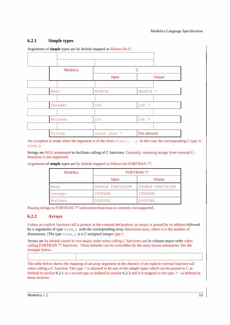
Modelica Language Specification
Modelica 1.2 53
6.2.1 Simple types
Arguments of simple types are by default mapped as follows for C:
CModelica
Input Output
Real double double *
Integer int int *
Boolean int int *
String const char * Not allowed.
An exception is made when the argument is of the form size(…, …) . In this case the corresponding C-type issize_t .
Strings are NUL-terminated to facilitate calling of C functions. Currently, returning strings from external C-functions is not supported.
Arguments of simple types are by default mapped as follows for FORTRAN 77:
FORTRAN 77Modelica
Input Output
Real DOUBLE PRECISION DOUBLE PRECISION
Integer INTEGER INTEGER
Boolean LOGICAL LOGICAL
Passing strings to FORTRAN 77 subroutines/functions is currently not supported.
6.2.2 Arrays
Unless an explicit function call is present in the external declaration, an arrays is passed by its address followedby n arguments of type size_t with the corresponding array dimension sizes, where n is the number ofdimensions. [The type size_t is a C unsigned integer type.]
Arrays are by default stored in row-major order when calling C functions and in column-major order whencalling FORTRAN 77 functions. These defaults can be overridden by the array layout annotation. See theexample below.
The table below shows the mapping of an array argument in the absence of an explicit external function callwhen calling a C function. The type T is allowed to be any of the simple types which can be passed to C asdefined in section 6.2.1 or a record type as defined in section 6.2.3 and it is mapped to the type T’ as defined inthese sections.
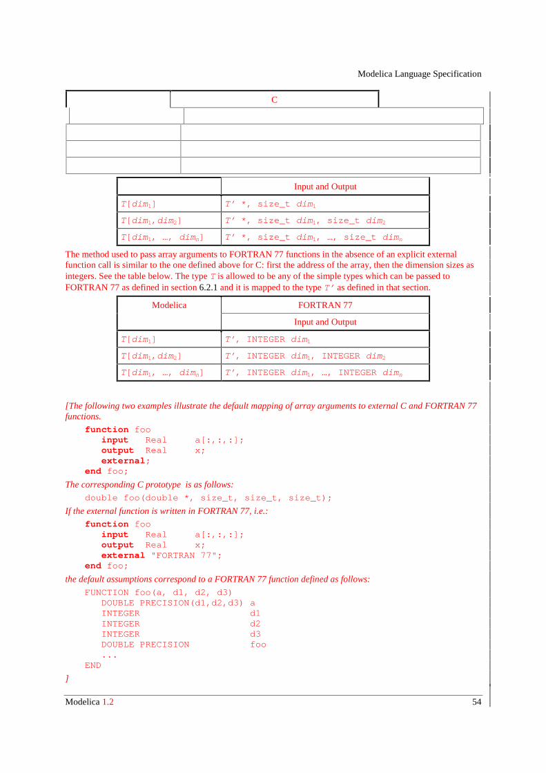
Modelica Language Specification
Modelica 1.2 54
C
Input and Output
T[dim1] T’ *, size_t dim 1
T[dim 1,dim 2] T’ *, size_t dim 1, size_t dim 2
T[dim 1, …, dimn] T’ *, size_t dim 1, …, size_t dimn
The method used to pass array arguments to FORTRAN 77 functions in the absence of an explicit externalfunction call is similar to the one defined above for C: first the address of the array, then the dimension sizes asintegers. See the table below. The type T is allowed to be any of the simple types which can be passed toFORTRAN 77 as defined in section 6.2.1 and it is mapped to the type T’ as defined in that section.
FORTRAN 77Modelica
Input and Output
T[dim 1] T’ , INTEGER dim 1
T[dim 1,dim 2] T’ , INTEGER dim 1, INTEGER dim 2
T[dim 1, …, dimn] T’ , INTEGER dim 1, …, INTEGER dimn
[The following two examples illustrate the default mapping of array arguments to external C and FORTRAN 77functions.
function foo input Real a[:,:,:]; output Real x; external;end foo;
The corresponding C prototype is as follows:
double foo(double *, size_t, size_t, size_t);
If the external function is written in FORTRAN 77, i.e.:
function foo input Real a[:,:,:]; output Real x; external "FORTRAN 77";end foo;
the default assumptions correspond to a FORTRAN 77 function defined as follows:
FUNCTION foo(a, d1, d2, d3) DOUBLE PRECISION(d1,d2,d3) a INTEGER d1 INTEGER d2 INTEGER d3 DOUBLE PRECISION foo ...END
]
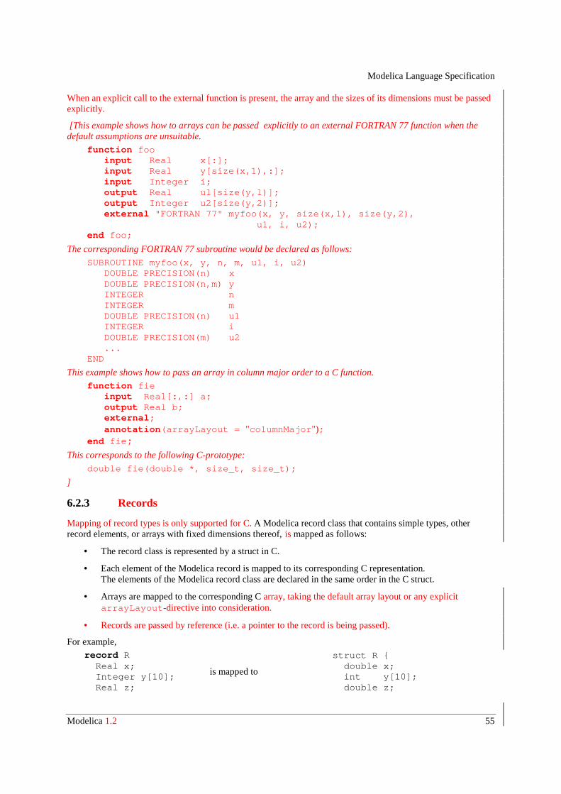
Modelica Language Specification
Modelica 1.2 55
When an explicit call to the external function is present, the array and the sizes of its dimensions must be passedexplicitly.
[This example shows how to arrays can be passed explicitly to an external FORTRAN 77 function when thedefault assumptions are unsuitable.
function foo input Real x[:]; input Real y[size(x,1),:]; input Integer i; output Real u1[size(y,1)]; output Integer u2[size(y,2)]; external "FORTRAN 77" myfoo(x, y, size(x,1), size(y,2), u1, i, u2);end foo;
The corresponding FORTRAN 77 subroutine would be declared as follows:
SUBROUTINE myfoo(x, y, n, m, u1, i, u2) DOUBLE PRECISION(n) x DOUBLE PRECISION(n,m) y INTEGER n INTEGER m DOUBLE PRECISION(n) u1 INTEGER i DOUBLE PRECISION(m) u2 ...END
This example shows how to pass an array in column major order to a C function.
function fie input Real[:,:] a; output Real b; external; annotation(arrayLayout = "columnMajor");end fie;
This corresponds to the following C-prototype:
double fie(double *, size_t, size_t);
]
6.2.3 Records
Mapping of record types is only supported for C. A Modelica record class that contains simple types, otherrecord elements, or arrays with fixed dimensions thereof, is mapped as follows:
• The record class is represented by a struct in C.
• Each element of the Modelica record is mapped to its corresponding C representation.The elements of the Modelica record class are declared in the same order in the C struct.
• Arrays are mapped to the corresponding C array, taking the default array layout or any explicitarrayLayout-directive into consideration.
• Records are passed by reference (i.e. a pointer to the record is being passed).
For example,record R Real x; Integer y[10]; Real z;
is mapped to
struct R { double x; int y[10]; double z;
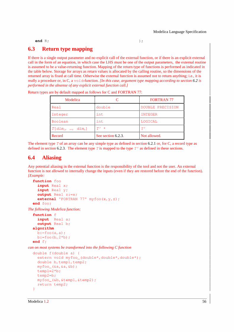
Modelica Language Specification
Modelica 1.2 56
end R; };
6.3 Return type mapping
If there is a single output parameter and no explicit call of the external function, or if there is an explicit externalcall in the form of an equation, in which case the LHS must be one of the output parameters, the external routineis assumed to be a value-returning function. Mapping of the return type of functions is performed as indicated inthe table below. Storage for arrays as return values is allocated by the calling routine, so the dimensions of thereturned array is fixed at call time. Otherwise the external function is assumed not to return anything; i.e., it isreally a procedure or, in C, a void-function. [In this case, argument type mapping according to section 6.2 isperformed in the absense of any explicit external function call.]
Return types are by default mapped as follows for C and FORTRAN 77:
Modelica C FORTRAN 77
Real double DOUBLE PRECISION
Integer int INTEGER
Boolean int LOGICAL
T[dim1, …, dimn] T’ * T’
Record See section 6.2.3. Not allowed.
The element type T of an array can be any simple type as defined in section 6.2.1 or, for C, a record type asdefined in section 6.2.3. The element type T is mapped to the type T’ as defined in these sections.
6.4 Aliasing
Any potential aliasing in the external function is the responsibility of the tool and not the user. An externalfunction is not allowed to internally change the inputs (even if they are restored before the end of the function).[Example:
function foo input Real x; input Real y; output Real z:=x; external "FORTRAN 77" myfoo(x,y,z); end foo;
The following Modelica function:
function f input Real a; output Real b; algorithm b:=foo(a,a); b:=foo(b,2*b); end f;
can on most systems be transformed into the following C function
double f(double a) { extern void myfoo_(double*,double*,double*); double b,temp1,temp2; myfoo_(&a,&a,&b); temp1=2*b; temp2=b; myfoo_(&b,&temp1,&temp2); return temp2; }
Modelica Language Specification
Modelica 1.2 57
The reason for not allowing the external function to change the inputs is to ensure that inputs can be stored instatic memory and to avoid superfluous copying (especially of matrices). If the routine does not satisfy therequirements the interface must copy the input argument to a temporary. This is rare but occurs e.g. in dormlq insome Lapack implementations. In those special cases the writer of the external interface have to copy the inputto a temporary. If the first input was changed internally in myfoo the designer of the interface would have tochange the interface function “foo” to:
function foo input Real x; protected Real xtemp:=x; // Temporary used because myfoo changes its input input Real y; output Real z; external "FORTRAN 77" myfoo(xtemp,y,z);end foo;
Note that we discuss input arguments for Fortran-routines even though Fortran 77 does not formally have inputarguments and forbid aliasing between any pair of arguments to a function (section 15.9.3.6 of X3J3/90.4). Forthe few (if any) Fortran 77 compilers that stricly follow the standard and are unable to handle aliasing betweeninput variables the tool must transform the first call of foo into
temp1=a; /* Temporary to avoid aliasing */ myfoo_(&a,&temp1,&b);
The use of the function foo in Modelica is unfluenced by these considerations.]
6.5 Examples
6.5.1 Input parameters, function value
[Here all parameters to the external function are input parameters. One function value is returned. If theexternal language is not specified, the default is "C", as below.
function foo input Real x; input Integer y; output Real w; external;end foo;
This corresponds to the following C-prototype:
double foo(double, int);
Example call in Modelica:
z = foo(2.4, 3);
Translated call in C:
z = foo(2.4, 3);
6.5.2 Arbitrary placement of output parameters, no external function value
In the following example, the external function call is given explicitly which allows passing the arguments in adifferent order than in the Modelica version.
function foo input Real x; input Integer y; output Real u1; output Integer u2; external "C" myfoo(x, u1, y, u2);end foo;
This corresponds to the following C-prototype:
void myfoo(double, double *, int, int *);
Modelica Language Specification
Modelica 1.2 58
Example call in Modelica:
(z1,i2) = foo(2.4, 3);
Translated call in C:
myfoo(2.4, &z1, 3, &i2);
6.5.3 External function with both function value and output variable
The following external function returns two results: one function value and one output parameter value. Bothare mapped to Modelica output parameters.
function foo input Real x; input Integer y; output Real funcvalue; output Integer out1; external "C" funcvalue = myfoo(x, y, out1);end foo;
This corresponds to the following C-prototype:
double myfoo(double, int, int *);
Example call in Modelica:
(z1,i2) = foo(2.4, 3);
Translated call in C:
z1 = myfoo(2.4, 3, &i2);
]
Modelica Language Specification
Modelica 1.2 59
7 Modelica standard library
The pre-defined, free "package Modelica" is shipped together with a Modelica translator. It is an extensivestandard library of pre-defined components in several domains. Futhermore, it contains a standard set of typeand interface definitions in order to influence the trivial decisions of model design process. If, as far as possible,standard quantity types and connectors are relied on in modeling work, model compatibility and thereby reuse isenhanced. Achieving model compatibility, without having to resort to explicit coordination of modelingactivities, is essential to the formation of globally accessible libraries. Naturally, a modeller is not required to usethe standard library and may also add any number of local base definitions.
The library will be amended and revised as part of the ordinary language revision process. It is expected thatinformal standard base classes will develop in various domains and that these gradually will be incorporated intothe Modelica standard library.
The type definitions in the library are based on ISO 31-1992. Several ISO quantities have long names that tendto become awkward in practical modeling work. For this reason, shorter alias-names are also provided ifnecessary. Using, e.g., "ElectricPotential" repeatedly in a model becomes cumbersome and therefore "Voltage"is also supplied as an alternative.
The standard library is not limited to pure SI units. Whenever common engineering practice uses a different setof (possibly inconsistent) units, corresponding quantities will be allowed in the standard library, for exampleEnglish units. It is also frequently common to write models with respect to scaled SI units in order to improvethe condition of the model equations or to keep the actual values around one for easier reading and writing ofnumbers.
The connectors and partial models have predefined graphical attributes in order that the basic visual appearanceis the same in all Modelica based systems.
The complete Modelica package can be downloaded. Below, the introductory documentation of this library isgiven together with links to the subpackages. Note, that the Modelica package is still under development.
package Modelica package Info /* The Modelica package is a standardized, pre-defined and free package, that is shipped together with a Modelica translator. The package provides constants, types, connectors, partial models and model components in various disciplines.
In the Modelica package the following conventions are used:
- Class and instance names are written in upper and lower case letters, e.g., "ElectricCurrent". An underscore is only used at the end of a name to characterize a lower or upper index, e.g., body_low_up.
- Type names start always with an upper case letter. Instance names start always with a lower case letter with only a few exceptions, such as "T" for a temperature instance.
- A package XXX has its interface definitions in subpackage XXX.Interface, e.g., Electric.Interface.
- Preferred instance names for connectors:
Modelica Language Specification
Modelica 1.2 60
p,n: positive and negative side of a partial model. a,b: side "a" and side "b" of a partial model (= connectors are completely equivalent).
The following subpackages are available:
GENERAL PACKAGES Constant Mathematical and physical constants Math Mathematical functions SIunit SI-unit type definitions
FORMALISM PACKAGES BlockDiagram Input/output blocks BondGraph Bond graph components FiniteStateMachine Finite state machine PetriNet One-token petri-nets. GENERAL DOMAINS Electric Electric and electronic components Mechanics 1D and 3D mechanical components ThermoFluid 1D thermo-fluid components
DOMAIN PACKAGES Aircraft Aircraft components Building Energy balance of building components DriveTrain Planetary gearboxes, clutches ElectricPower Generators, motors, electric line Hydraulics Hydraulic components */ end Info;end Modelica;