Modelling community evacuation vulnerability …content.csbs.utah.edu/~cova/cova-church-1997.pdfint. j. geographical information science,1997,vol.11,no.8,763±784 Research Article

int. j. geographical information science, 1997, vol. 11, no. 8, 763 ± 784

Research Article

Modelling community evacuation vulnerability using GIS

THOMAS J. COVA and RICHARD L. CHURCHNational Center for Geographic Information and Analysis (NCGIA),Department of Geography, University of California, Santa Barbara, SantaBarbara, California 93106, USAemail: [email protected]

(Received 26 June 1996; accepted 10 February 1997 )

Abstract. We present a method for systematically identifying neighbourhoodsthat may face transportation diYculties during an evacuation. A classi® cation ofthis nature oVers a unique approach to assessing community vulnerability inregions subject to fast-moving hazards of uncertain spatial impact (e.g., urban® restorms and toxic spills on highways) . The approach is founded on an integerprogramming ( IP) model called the critical cluster model (CCM). An heuristicalgorithm is described which is capable of producing eYcient, high-quality solu-tions to this model in a GIS context. The paper concludes with an application ofthe method to Santa Barbara, California.

1. Introduction

The ® eld of regional evacuation modelling has evolved along a fundamentallytemporal line of inquiry, where research has centred on the problem of accuratelyestimating the time it might take to clear a speci® ed zone of its population. Thisfocus was initially motivated by the perceived threat imposed by nuclear powerplants during the 1970s (WSA 1974 ), and the accidents at Pennsylvania’s Three MileIsland in 1979 and Chernobyl in 1986 served to reinforce this emphasis. The generalapproach involved prede® ning a circular emergency planning zone (EPZ) aroundeach nuclear site using a 10-mile radius (NRC 1980, Urbanik et al. 1980 ) andsubsequently pursuing an estimate of the time it might take to clear the zone. Earlystatic-analysis techniques for estimating network clearance time (WSA 1974, Stone1983) have since been eclipsed by special-purpose transportation simulation modelscapable of dynamically modelling evacuations on the scale of entire urban areas(SheY et al. 1982, FEMA 1984, Hobeika and Jamei 1985, Pidd et al. 1996). Anumber of these simulation models have become the basis for evacuation decisionsupport systems (Han 1990, Tufekci and Kisko 1991, de Silva et al. 1993, Hobeikaet al. 1994).

In the wake of this early evacuation research on nuclear power plants, a modellingparadigm emerged (Southworth 1991, Urbanik and Jamison 1992). The standardapproach was to delimit an EPZ around a known hazard and subsequently applyan evacuation simulation model to explore questions regarding the many factorsthat might aVect network clearance time (e.g., routing, population distribution, roadand intersection capacity, human behaviour). This general approach proved veryuseful and has been used to model the evacuation of communities at risk to chemical

1365± 8816/97 $12´00 Ñ 1997 Taylor & Francis Ltd.

T . J. Cova and R. L . Church764

stockpile sites (Newsom et al. 1992 ), nuclear research facilities (Sinuany-Sternand Stern 1993), dams (Southworth and Chin 1987), and hurricanes (Hobeikaet al. 1985).

A key concept that underlies this modelling approach is the notion of a credibleEPZ. A credible EPZ is a valuable spatial construct, as it provides a crisp answerto the dual questions of who needs to be evacuated (population in the zone) andwhere they need to be routed to reach safety (outside the zone). In a sense, it servesas a formal agreement among emergency planners regarding the de® nition of a likelyevacuation. This allows analysts to move directly to issues related to estimating andreducing the time it might take to clear a zone. As Sorensen et al. (1992) note,delimiting a credible EPZ can be a signi® cant political and technical endeavour forcertain hazard types.

However, a problem arises when an analyst is faced with performing an evacu-ation assessment for a region that is subject to a hazard with a high degree ofuncertainty in its spatial impact. In short, there are many hazards where the popula-tion to be evacuated simply cannot be determined in advance. Urban ® restorms,toxic spills on highways, and many other hazards routinely result in ad hoc evacuationzones that are established at the time of the event. For this reason, hazards with ahigh degree of spatial uncertainty pose an interesting modelling problem. We callthis problem the indeterminable EPZ problem (IEPZ) and state it as follows: Howcan an evacuation assessment be performed when the population to evacuate is anunknown (i.e., when a credible EPZ cannot be established in advance)?

As the IEPZ problem is a spatial problem, it represents a signi® cant opportunityto utilize a GIS approach. The potential role for GIS in evacuation research hasbeen noted by a number of authors (Gatrell and Vincent 1991, Dangermond 1991,Johnson 1992, Rejeski 1993 ), but little work has been done in this area to date. GIShave been applied in generating alternative evacuation routes out of a given zone(Dangermond 1985, Dunn 1992) and in managing the spatial data associated withan evacuation decision support system (de Silva et al. 1993). In general, the widerapplication of GIS in hazards research has focused on modelling the physical aspectsof hazards (Wadge 1988, Chou 1992, Shu-Quiang and Unwin 1992, Carrara andGuzzetti 1995, Emmi and Horton 1995, Radke 1995) and not on potential evacuationdiYculties. Although evacuation vulnerability modelling is clearly related to GISnatural hazards research, it’s more closely aligned with GIS research on modellinghuman vulnerability and risk (McMaster 1988, Estes et al. 1987, Hodgson and Palm1992, Burke 1993, Emani et al. 1993, Brainard et al. 1996).

The purpose of this paper is to describe a GIS approach to the problem ofidentifying neighbourhoods that may face transportation diYculties during an evacu-ation. A secondary concern is to demonstrate that the algorithm underlying thisapproach is a candidate for addition to the spatial analytic toolbox of contemporaryGIS (Goodchild 1987, Burrough 1990, Fotheringham and Rogerson 1993). The paperbegins with a description of a methodological framework designed to address theIEPZ problem that we call evacuation vulnerability modelling. A fundamental prob-lem is identi® ed and formulated as an integer programming (IP) model. Solving thisIP model optimally is impractical for most real-world road networks, and we describea heuristic algorithm designed to produce eYcient, high-quality solutions to themodel in a GIS context. An application of the method is presented for Santa Barbara,California, and the paper ® nishes with a conclusion and discussion of further research.

Modelling evacuation vulnerability 765

2. Evacuation vulnerability modelling

An initial approach to addressing the IEPZ problem is to shift the emphasisfrom a temporal to a spatial perspective. Rather than pursuing the question as tothe time it might take to clear a single zone under a particular hazard, regionalevacuation can be viewed as a generic process (Perry 1985) independent of anyhazard or zone. In other words, clearing people from an area can be viewed as aprocess independent of any particular zone or hazardous event that might warrantthe evacuation. From this perspective, there would be an extremely large number ofpotential evacuations in any given region. An interesting problem involves classi-fying them regarding transportation diYculties that might arise during an urgentevacuation (e.g., congestion).

Essentially, we require a measure of evacuation diYculty at each point in theplane. One approach is to ® nd a zone for each point that (1) contains the point, (2)is limited in size, and (3) represents the most diYcult evacuation for that point. Ifthis process was performed on a network data model at select points (i.e., inter-sections), it would be possible to produce a ® eld de® ned along the network thatrepresents an upper bound on potential transportation evacuation diYculties.Goodchild (1992 ) would consider this a process of generating a ® eld from a discretedata model. A ® eld of this nature would aid in assessing vulnerability, as communitiesthat are unable to clear their immediate locale in a safe and timely manner may leadto disastrous consequences in some hazard contexts (OFD 1992).

2.1. All possible evacuationsRegional evacuation is a human process that occurs at the level of the individual,

and it is assumed that there are a ® nite number of individuals in any de® ned regionat a given point in time. As such, a set theoretic view can be adopted, where anevacuation is de® ned as any subset of a region’s population clearing its immediatelocale. The extent of the evacuation is thereby de® ned by the extent of the populationinvolved. With time ® xed (time-slice), there are a ® nite number of potential evacu-ations, as there are a ® nite number of subsets of any ® nite set. The cardinality ofthis set is given in equation (1) where n is the population of the study area and E isthe set of all evacuations.

|E|= �n

i=1A n

i B (1 )

For an area with a population as small as 50, there would be greater than1015 potential evacuations (population subsets) at any point in time. A reductionof this set is required to move this problem into a computationally tractabledomain (GIS).

First, the case where the evacuees are not in proximity is highly unlikely, andcontiguity can be added to the de® nition of a valid evacuation. That is, the populationmust come from a contiguous area. Second, the most critical population to evacuatein the context of fast-moving hazards of uncertain spatial impact is the populationwithin immediate proximity to the origin of the event. To focus on these frequent(Sorensen et al. 1987) micro-evacuations, a size limit can be included in the de® nitionof a valid evacuation. Lastly, it’s impossible to geo-reference all individuals within astudy area, and a common aggregate geographic representation of population must


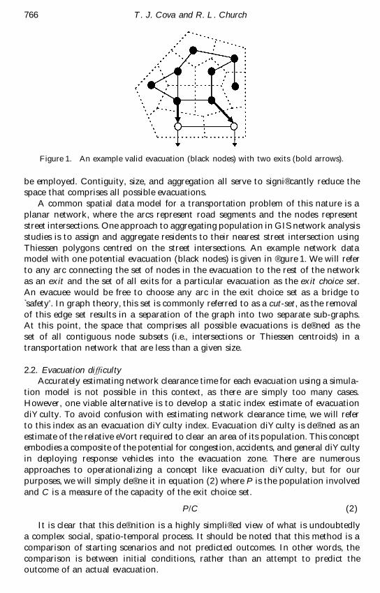
Figure 1. An example valid evacuation (black nodes) with two exits (bold arrows).

be employed. Contiguity, size, and aggregation all serve to signi® cantly reduce thespace that comprises all possible evacuations.

A common spatial data model for a transportation problem of this nature is aplanar network, where the arcs represent road segments and the nodes representstreet intersections. One approach to aggregating population in GIS network analysisstudies is to assign and aggregate residents to their nearest street intersection usingThiessen polygons centred on the street intersections. An example network datamodel with one potential evacuation (black nodes) is given in ® gure 1. We will referto any arc connecting the set of nodes in the evacuation to the rest of the networkas an exit and the set of all exits for a particular evacuation as the exit choice set.An evacuee would be free to choose any arc in the exit choice set as a bridge tosafety’. In graph theory, this set is commonly referred to as a cut-set, as the removalof this edge set results in a separation of the graph into two separate sub-graphs.At this point, the space that comprises all possible evacuations is de® ned as theset of all contiguous node subsets (i.e., intersections or Thiessen centroids) in atransportation network that are less than a given size.

2.2. Evacuation diYcultyAccurately estimating network clearance time for each evacuation using a simula-

tion model is not possible in this context, as there are simply too many cases.However, one viable alternative is to develop a static index estimate of evacuationdiYculty. To avoid confusion with estimating network clearance time, we will referto this index as an evacuation diYculty index. Evacuation diYculty is de® ned as anestimate of the relative eVort required to clear an area of its population. This conceptembodies a composite of the potential for congestion, accidents, and general diYcultyin deploying response vehicles into the evacuation zone. There are numerousapproaches to operationalizing a concept like evacuation diYculty, but for ourpurposes, we will simply de® ne it in equation (2) where P is the population involvedand C is a measure of the capacity of the exit choice set.

P/C (2 )

It is clear that this de® nition is a highly simpli® ed view of what is undoubtedlya complex social, spatio-temporal process. It should be noted that this method is acomparison of starting scenarios and not predicted outcomes. In other words, thecomparison is between initial conditions, rather than an attempt to predict theoutcome of an actual evacuation.


2.3. Spatial evacuation vulnerabilityWith the space that comprises all possible evacuations de® ned and an approach

to scoring their potential diYculty, the focus can shift to developing a systematicspatial classi® cation method. One approach is to inquire as to the worst-case (i.e.,maximum diYculty) that each node in a network might be involved in, less than acertain size. We call this worst-case for a particular node (and size limit) its spatialevacuation vulnerability . The primary task is, then, to map the local variation inevacuation vulnerability throughout a network due to the unique geographicalsetting of individual nodes.

The de® nition of worst-case’ in this context refers to the maximum value for agiven diYculty measure and not the actual worst-case that might occur. For example,an actual evacuation could easily be more diYcult due to the loss of exits (e.g.,hazard or stalled vehicle), signi® cant imbalances in the number of evacuees utilizingvarious exits, or convergence on the hazard site by response personnel and localcitizens. The de® nition of worst-case utilized in this paper is simply an attempt tosystematically reveal the geographical context in which an evacuation might takeplace.

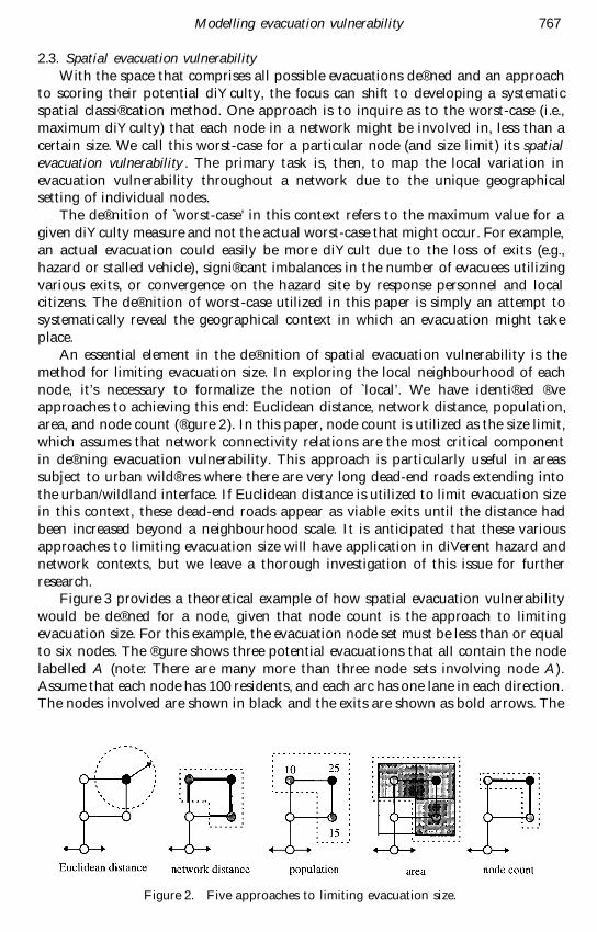
An essential element in the de® nition of spatial evacuation vulnerability is themethod for limiting evacuation size. In exploring the local neighbourhood of eachnode, it’s necessary to formalize the notion of local’. We have identi® ed ® veapproaches to achieving this end: Euclidean distance, network distance, population,area, and node count ( ® gure 2). In this paper, node count is utilized as the size limit,which assumes that network connectivity relations are the most critical componentin de® ning evacuation vulnerability. This approach is particularly useful in areassubject to urban wild® res where there are very long dead-end roads extending intothe urban/wildland interface. If Euclidean distance is utilized to limit evacuation sizein this context, these dead-end roads appear as viable exits until the distance hadbeen increased beyond a neighbourhood scale. It is anticipated that these variousapproaches to limiting evacuation size will have application in diVerent hazard andnetwork contexts, but we leave a thorough investigation of this issue for furtherresearch.

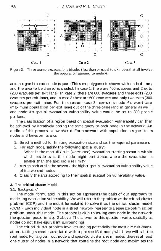
Figure 3 provides a theoretical example of how spatial evacuation vulnerabilitywould be de® ned for a node, given that node count is the approach to limitingevacuation size. For this example, the evacuation node set must be less than or equalto six nodes. The ® gure shows three potential evacuations that all contain the nodelabelled A (note: There are many more than three node sets involving node A) .Assume that each node has 100 residents, and each arc has one lane in each direction.The nodes involved are shown in black and the exits are shown as bold arrows. The

Figure 2. Five approaches to limiting evacuation size.


Figure 3. Three example evacuations (shaded) less than or equal to six nodes that all involvethe population assigned to node A.

area assigned to each node (square Thiessen polygons) is shown with dashed lines,and the area to be cleared is shaded. In case 1, there are 400 evacuees and 2 exits(200 evacuees per exit lane). In case 2, there are 600 evacuees and three exits (200evacuees per exit lane), and in case 3 there are 600 evacuees and only two exits (300evacuees per exit lane) . For this reason, case 3 represents node A’s worst-case(maximum population per exit lane) out of the three cases (and in general as well ),and node A’s spatial evacuation vulnerability value would be set to 300 peopleper lane.

The classi® cation of a region based on spatial evacuation vulnerability can thenbe achieved by iteratively posing the same query to each node in the network. Anoutline of this process is now oVered. For a network with population assigned to itsnodes and lanes on its arcs:

1. Select a method for limiting evacuation size and set the required parameters.2. For each node, satisfy the following spatial query:

`What is the most diYcult (worst-case) evacuation starting scenario withinwhich residents at this node might participate, where the evacuation issmaller than the speci® ed size limit?’

3. Assign each arc in the network the higher spatial evacuation vulnerability valueof its two end nodes.

4. Classify the arcs according to their spatial evacuation vulnerability value.

3. The critical cluster model

3.1. Backgrou ndThe model formulated in this section represents the basis of our approach to

modelling evacuation vulnerability. We will refer to the problem as the critical clusterproblem (CCP) and the model formulated to solve it as the critical cluster model(CCM ). Each individual node in a street network represents a separate optimizationproblem under this model. The process is akin to asking each node in the networkthe question posed in step 2 above. The answer to this question varies spatially asnodes do not have equivalent surroundings.

The critical cluster problem involves ® nding potentially the most diYcult evacu-ation starting scenario associated with a pre-speci® ed node, which we will call theroot node. For a given root node and speci® ed cluster size in nodes, there is at leastone cluster of nodes in a network that contains the root node and maximizes the


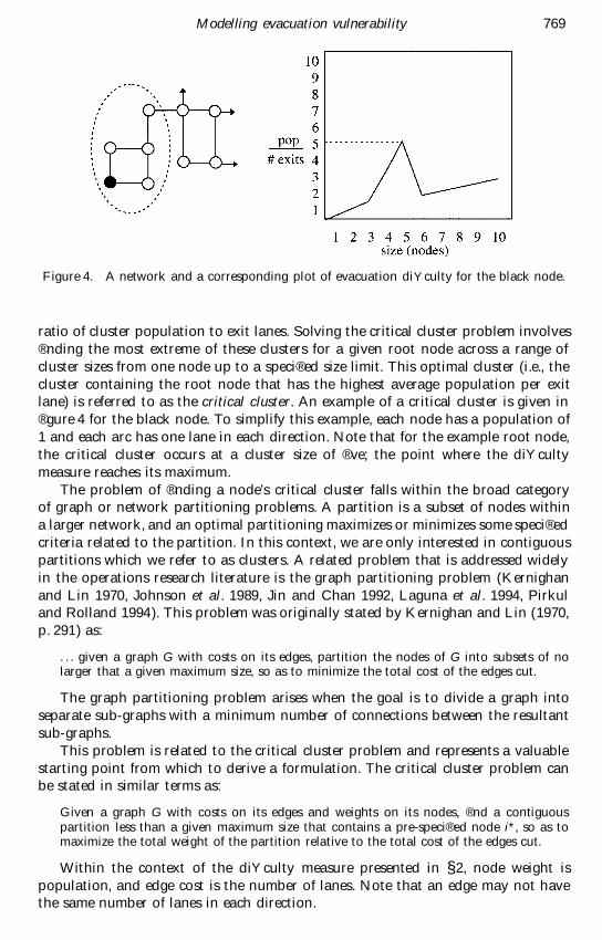
Figure 4. A network and a corresponding plot of evacuation diYculty for the black node.

ratio of cluster population to exit lanes. Solving the critical cluster problem involves® nding the most extreme of these clusters for a given root node across a range ofcluster sizes from one node up to a speci® ed size limit. This optimal cluster (i.e., thecluster containing the root node that has the highest average population per exitlane) is referred to as the critical cluster. An example of a critical cluster is given in® gure 4 for the black node. To simplify this example, each node has a population of1 and each arc has one lane in each direction. Note that for the example root node,the critical cluster occurs at a cluster size of ® ve; the point where the diYcultymeasure reaches its maximum.

The problem of ® nding a node’s critical cluster falls within the broad categoryof graph or network partitioning problems. A partition is a subset of nodes withina larger network, and an optimal partitioning maximizes or minimizes some speci® edcriteria related to the partition. In this context, we are only interested in contiguouspartitions which we refer to as clusters. A related problem that is addressed widelyin the operations research literature is the graph partitioning problem (Kernighanand Lin 1970, Johnson et al. 1989, Jin and Chan 1992, Laguna et al. 1994, Pirkuland Rolland 1994). This problem was originally stated by Kernighan and Lin (1970,p. 291) as:

. . . given a graph G with costs on its edges, partition the nodes of G into subsets of nolarger that a given maximum size, so as to minimize the total cost of the edges cut.

The graph partitioning problem arises when the goal is to divide a graph intoseparate sub-graphs with a minimum number of connections between the resultantsub-graphs.

This problem is related to the critical cluster problem and represents a valuablestarting point from which to derive a formulation. The critical cluster problem canbe stated in similar terms as:

Given a graph G with costs on its edges and weights on its nodes, ® nd a contiguouspartition less than a given maximum size that contains a pre-speci® ed node i*, so as tomaximize the total weight of the partition relative to the total cost of the edges cut.

Within the context of the diYculty measure presented in § 2, node weight ispopulation, and edge cost is the number of lanes. Note that an edge may not havethe same number of lanes in each direction.


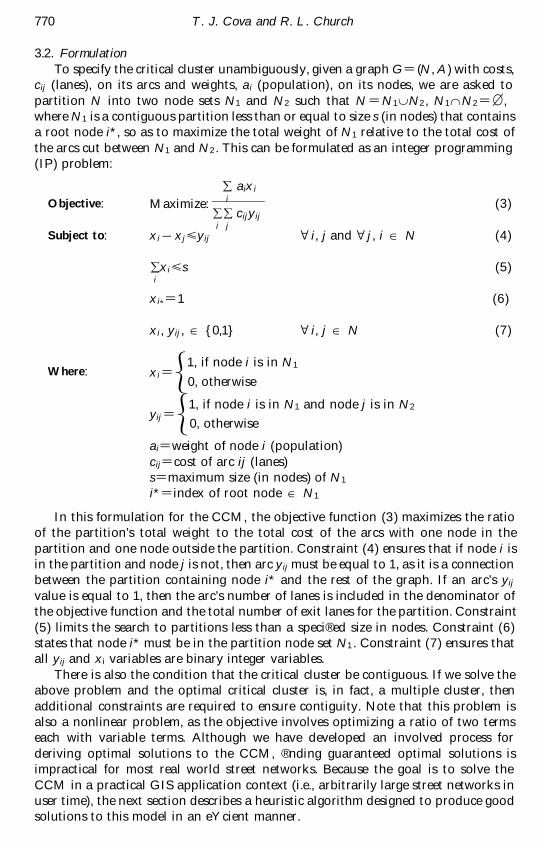
3.2. FormulationTo specify the critical cluster unambiguously, given a graph G= (N, A ) with costs,

cij ( lanes), on its arcs and weights, a i (population), on its nodes, we are asked topartition N into two node sets N1 and N2 such that N=N1nN2 , N1mN2=B,where N1 is a contiguous partition less than or equal to size s (in nodes) that containsa root node i*, so as to maximize the total weight of N1 relative to the total cost ofthe arcs cut between N1 and N2 . This can be formulated as an integer programming(IP) problem:

Objective: (3 )Maximize:�i

aix i

�i�j

cijy ij

Subject to: x i Õ x j < y ij Y i, j and Y j , i × N (4 )

�ix i < s (5 )

x i*=1 (6)

x i , y ij , × {0,1} Y i, j × N (7 )

Where: x i=G1, if node i is in N1

0, otherwise

yij=G1, if node i is in N1 and node j is in N2

0, otherwise

ai=weight of node i (population)cij=cost of arc ij ( lanes)s=maximum size (in nodes) of N1

i*=index of root node × N1

In this formulation for the CCM, the objective function (3 ) maximizes the ratioof the partition’s total weight to the total cost of the arcs with one node in thepartition and one node outside the partition. Constraint (4) ensures that if node i isin the partition and node j is not, then arc y ij must be equal to 1, as it is a connectionbetween the partition containing node i* and the rest of the graph. If an arc’s yij

value is equal to 1, then the arc’s number of lanes is included in the denominator ofthe objective function and the total number of exit lanes for the partition. Constraint(5) limits the search to partitions less than a speci® ed size in nodes. Constraint (6)states that node i* must be in the partition node set N1 . Constraint (7) ensures thatall y ij and xi variables are binary integer variables.

There is also the condition that the critical cluster be contiguous. If we solve theabove problem and the optimal critical cluster is, in fact, a multiple cluster, thenadditional constraints are required to ensure contiguity. Note that this problem isalso a nonlinear problem, as the objective involves optimizing a ratio of two termseach with variable terms. Although we have developed an involved process forderiving optimal solutions to the CCM, ® nding guaranteed optimal solutions isimpractical for most real world street networks. Because the goal is to solve theCCM in a practical GIS application context (i.e., arbitrarily large street networks inuser time), the next section describes a heuristic algorithm designed to produce goodsolutions to this model in an eYcient manner.


4. Heuristic algorithm

4.1. DesignConceptually, the heuristic grows’ a cluster from a speci® ed root node in a

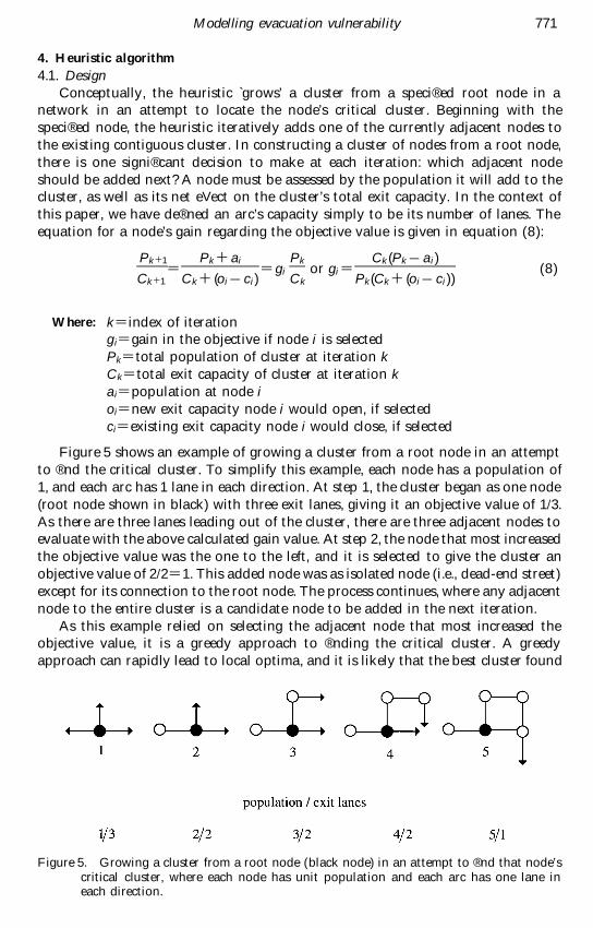
network in an attempt to locate the node’s critical cluster. Beginning with thespeci® ed node, the heuristic iteratively adds one of the currently adjacent nodes tothe existing contiguous cluster. In constructing a cluster of nodes from a root node,there is one signi® cant decision to make at each iteration: which adjacent nodeshould be added next? A node must be assessed by the population it will add to thecluster, as well as its net eVect on the cluster’s total exit capacity. In the context ofthis paper, we have de® ned an arc’s capacity simply to be its number of lanes. Theequation for a node’s gain regarding the objective value is given in equation (8):

Pk+1

Ck+1=

Pk+ai

Ck+ (o i Õ ci )=gi

Pk

Ckor gi=

Ck (Pk Õ a i )

Pk (Ck+ (o i Õ ci ))(8 )

Where: k=index of iterationg i=gain in the objective if node i is selectedPk=total population of cluster at iteration kCk=total exit capacity of cluster at iteration ka i=population at node io i=new exit capacity node i would open, if selectedci=existing exit capacity node i would close, if selected

Figure 5 shows an example of growing a cluster from a root node in an attemptto ® nd the critical cluster. To simplify this example, each node has a population of1, and each arc has 1 lane in each direction. At step 1, the cluster began as one node(root node shown in black) with three exit lanes, giving it an objective value of 1/3.As there are three lanes leading out of the cluster, there are three adjacent nodes toevaluate with the above calculated gain value. At step 2, the node that most increasedthe objective value was the one to the left, and it is selected to give the cluster anobjective value of 2/2=1. This added node was as isolated node (i.e., dead-end street)except for its connection to the root node. The process continues, where any adjacentnode to the entire cluster is a candidate node to be added in the next iteration.

As this example relied on selecting the adjacent node that most increased theobjective value, it is a greedy approach to ® nding the critical cluster. A greedyapproach can rapidly lead to local optima, and it is likely that the best cluster found

Figure 5. Growing a cluster from a root node (black node) in an attempt to ® nd that node’scritical cluster, where each node has unit population and each arc has one lane ineach direction.


by this approach will not be optimal. However, solution quality can be greatlyimproved by modifying the procedure to use a semi-greedy approach. In a semi-greedy approach, an alpha parameter (expressed as a percentage) is used to increasethe possible list of adjacent nodes that might be selected to add to the cluster. Inshort, the improvement factor for all adjacent nodes is calculated using equation (8),and all adjacent nodes are scanned again to produce a list of only the ones that aregreater than alpha per cent of the best option. This implies that nodes with gainvalues less than the best node may be possible candidates for selection. A randomselection is made from this list of candidate additions at each step. For this reason,successive runs of the heuristic for a given root node will likely result in diVerentresults. A second parameter (starts) can be added to control the number of timeseach node is run, where the best overall objective value is saved.

In addition to semi-greedy selection, we add the concept of adaptiveness foundin the GRASP approach (Laguna et al. 1994). Adaptiveness is an answer to thenotion that selecting one adjacent node can change the gain value of other adjacentnodes. In short, selecting one node aVects the relative scores of all other adjacentnodes. This has a signi® cant impact on the complexity of the algorithm, as it impliesthat the gain values for all adjacent nodes must be recalculated after every nodeselection. In this way, the nodes are thought to adapt their respective gain values tothe changing state of the cluster.

4.2. Implementation4.2.1. GIS considerations

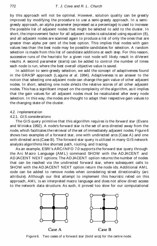
The GIS query primitive that this algorithm requires is the forward star (Evansand Minieka 1992). A node’s forward star is the set of arcs directed away from thenode, which facilitates the retrieval of the set of immediately adjacent nodes. Figure 6shows two examples of a forward star, one with undirected arcs (Case A) and onewith directed arcs (Case B). The forward star query is utilized in many GIS networkanalysis algorithms like shortest path, routing, and tracing.

As an example, ESRI’s ARC/INFO 7.0 supports the forward star query throughthe Arc Macro Language (AML) command SHOW with the ADJACENT andADJACENT NEXT options. The ADJACENT option returns the number of nodesthat can be reached via the undirected forward star, where subsequent calls toSHOW with the ADJACENT NEXT option return the node ids. Additional AMLcode can be added to remove nodes when considering street directionality (arcattribute). Although our ® rst attempt to implement this heuristic relied on thisapproach, AML is an interpreted macro language and does not allow direct accessto the network data structure. As such, it proved too slow for our computational

Figure 6. Two cases of a forward star (bold arcs) for the centre node.


experimental design, as we wanted to be able to grow many clusters from each nodein a network of more than 5000 nodes using a variety of alternatives regarding thedecision of which node to add at each step. For this reason, we implemented ourown forward star network data structure (Evans and Minieka 1992) in a stand-aloneC program and loosely coupled the program with ARC/INFO by exporting thenetwork to text and importing the heuristic results back into ARC/INFO. In anenvironment where a software engineer has access to the internals of the GIS networkdata structure, the forward star query could be optimized, and the heuristic couldbe run in user-time within the GIS. A compromise between these two engineeringextremes is ESRI’s ARCVIEW 3.0, which has support for the forward star querythrough a dynamic link library (DLL) that can be called directly from a compiledC program (Honeycutt 1996 ).

4.2.2. Speci® cationThe implementation of the heuristic takes as input a textual representation of a

network and a set of parameters, whereby it produces an output ® le of node id’sand their associated spatial evacuation vulnerability values. The parameters of theprogram are given in table 1.

There are two conditions that must be met before a network can be consideredvalid for an application of the heuristic: contiguity and global exit. Contiguity impliesthat there must exist at least one path between every pair of nodes in the network,and global exit implies that at least one node in the network be designated as anexit from the entire network. A global exit may not be selected as a component nodeof any cluster, and as most digital road networks are subsets of a larger network, itshould be clear which nodes represent exits from the network.

The main control logic behind the algorithm is given in ® gure 7 as pseudocode.

Figure 7. The pseudocode for the heuristic algorithm.


Given a size limit, the algorithm sequentially runs through the nodes in a network,in an attempt to ® nd the critical cluster for each node. The only required parameteris the size limit, as the subsequent parameters are only used to improve the qualityof the solutions produced by the algorithm. The total cluster weight over the numberof exit lanes is referred to as the weight/cost value.

An important bene® t of the structure of a critical cluster, in general, is that allthe nodes that comprise one must have a critical cluster weight/cost ratio at least aslarge as the original critical cluster’s. This means that when a maximum cluster isfound for a particular root node, the nodes that comprise this cluster that have acritical cluster weight/cost value less than this critical cluster’s value can automaticallybe raised up to this new value. It is still possible, however, for a subset of thesecomponent nodes to have an even higher critical cluster value. This improvementstrategy is listed as step (10).

4.3. EvaluationTo test the performance of the heuristic algorithm, optimal solutions to the CCM

were derived for 40 randomly selected nodes from 4 real-world street networks (10each) at three evacuation size limits 10, 25, and 50 (120 problems), where the networksranged in size from 200 to 300 nodes. The equation for evaluating the per cent fromoptimal for a node and size limit is:

O Õ B

O(9 )

where O is the optimal solution and B is the best solution achieved by the heuristic.Table 2 shows the mean per cent from optimal for the 120 problems for eachcombination of the semi-greedy parameters alpha and starts. A high alpha (e.g., near1) constrains the growth of the cluster to greedy, where lowering alpha results inprogressively wilder’ cluster growth. Note that for a starts of 1 (row 1), the solution

Table 1. Program parameters.

Name Range Description

Size limit 1 . . . n Õ 1 The size limit (in nodes) to terminate growthAlpha 0 . . . 1 The semi-greedy percentage parameterStarts 1 . . . x The number of times to start the heuristic from a root node

Table 2. Mean percentage from optimal varying alpha and starts ( 120 problems per cell ).

alphaStarts 0 975 0 950 0 925 0 900 0 875 0 850 0 825 0 800 0 775 0 750

1 12 07 10 53 11 21 11 61 11 01 12 69 12 04 15 14 15 42 17 672 10 57 8 56 9 32 9 14 10 23 9 52 10 27 11 18 13 06 11 934 9 53 7 13 8 16 7 75 7 47 8 08 8 03 8 51 9 97 8 598 7 72 6 12 5 92 5 08 6 73 5 92 7 35 6 82 6 65 8 04

16 7 72 6 12 5 92 5 08 6 73 5 92 7 35 6 82 6 65 8 0432 7 81 5 25 4 95 4 29 4 34 4 53 4 45 5 06 5 02 5 0264 6 58 4 85 4 48 3 77 4 32 3 84 4 15 4 2 3 81 3 93

128 6 58 4 74 4 13 3 95 3 69 3 87 3 61 4 02 2´99 3 72


quality decreases as alpha is decreased and the cluster growth gets wilder. Also, forall columns, solution quality improves as starts is increased. The best overall com-bination occurred at an alpha of 0 775 and a starts of 128, where the averagepercentage from optimal was 2 99. For our sample set of nodes, this implies that thebest combination for high solution quality is moderately wild cluster growth and alarge number of starts.

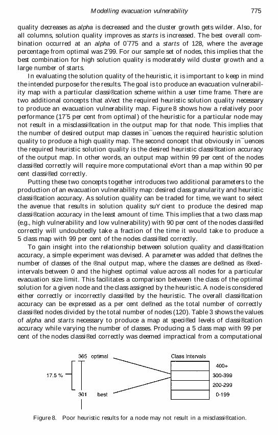
In evaluating the solution quality of the heuristic, it is important to keep in mindthe intended purpose for the results. The goal is to produce an evacuation vulnerabil-ity map with a particular classi® cation scheme within a user time frame. There aretwo additional concepts that aVect the required heuristic solution quality necessaryto produce an evacuation vulnerability map. Figure 8 shows how a relatively poorperformance (17 5 per cent from optimal ) of the heuristic for a particular node maynot result in a misclassi® cation in the output map for that node. This implies thatthe number of desired output map classes in¯ uences the required heuristic solutionquality to produce a high quality map. The second concept that obviously in¯ uencesthe required heuristic solution quality is the desired heuristic classi® cation accuracyof the output map. In other words, an output map within 99 per cent of the nodesclassi® ed correctly will require more computational eVort than a map within 90 percent classi® ed correctly.

Putting these two concepts together introduces two additional parameters to theproduction of an evacuation vulnerability map: desired class granularity and heuristicclassi® cation accuracy. As solution quality can be traded for time, we want to selectthe avenue that results in solution quality suYcient to produce the desired mapclassi® cation accuracy in the least amount of time. This implies that a two class map(e.g., high vulnerability and low vulnerability) with 90 per cent of the nodes classi® edcorrectly will undoubtedly take a fraction of the time it would take to produce a5 class map with 99 per cent of the nodes classi® ed correctly.

To gain insight into the relationship between solution quality and classi® cationaccuracy, a simple experiment was devised. A parameter was added that de® nes thenumber of classes of the ® nal output map, where the classes are de® ned as ® xed-intervals between 0 and the highest optimal value across all nodes for a particularevacuation size limit. This facilitates a comparison between the class of the optimalsolution for a given node and the class assigned by the heuristic. A node is consideredeither correctly or incorrectly classi® ed by the heuristic. The overall classi® cationaccuracy can be expressed as a per cent de® ned as the total number of correctlyclassi® ed nodes divided by the total number of nodes (120). Table 3 shows the valuesof alpha and starts necessary to produce a map at speci® ed levels of classi® cationaccuracy while varying the number of classes. Producing a 5 class map with 99 percent of the nodes classi® ed correctly was deemed impractical from a computational

Figure 8. Poor heuristic results for a node may not result in a misclassi® cation.


Table 3. Required (alpha, starts) pairs to produce a map at a speci® ed heuristic classi® cationaccuracy for a speci® ed number of classes.

Node classi® cation accuracy (per cent)

No. of classes 90 95 97 5 99

2 (0 95, 1 ) (0 95, 1) (0 95, 1) (0 95, 8)3 (0 95, 1 ) (0 95, 1) (0 95, 8) (0 95, 16)4 (0 95, 8 ) (0 95, 16) (0 775, 64) (0 775, 256)5 (0 90, 32 ) (0 775, 64 ) (0 75, 512) impractical

Figure 9. The relation between arc and node classi® cation accuracy.

perspective, as producing a map with 97 5 of the nodes classi® ed correctly required512 starts of the heuristic at each node in the network.

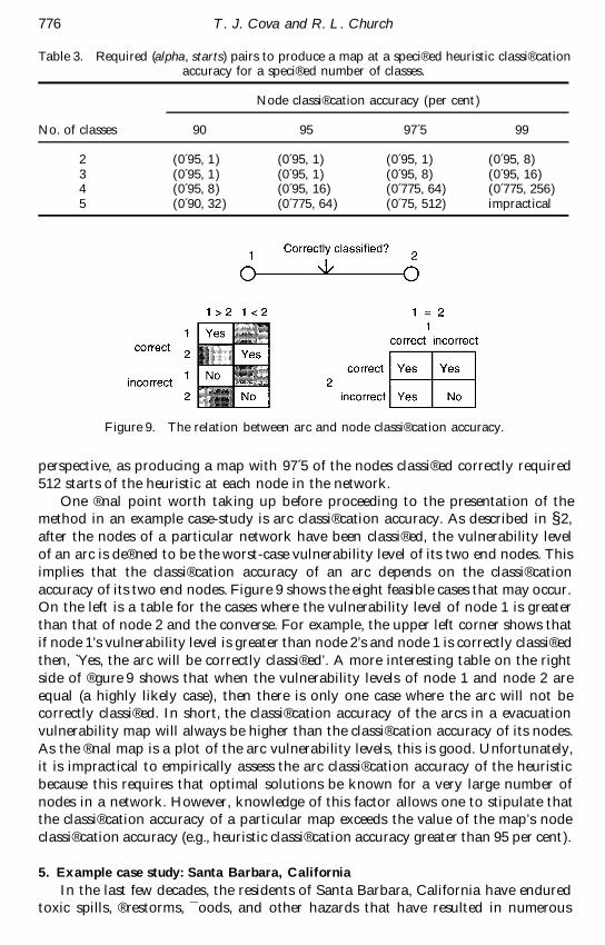
One ® nal point worth taking up before proceeding to the presentation of themethod in an example case-study is arc classi® cation accuracy. As described in § 2,after the nodes of a particular network have been classi® ed, the vulnerability levelof an arc is de® ned to be the worst-case vulnerability level of its two end nodes. Thisimplies that the classi® cation accuracy of an arc depends on the classi® cationaccuracy of its two end nodes. Figure 9 shows the eight feasible cases that may occur.On the left is a table for the cases where the vulnerability level of node 1 is greaterthan that of node 2 and the converse. For example, the upper left corner shows thatif node 1’s vulnerability level is greater than node 2’s and node 1 is correctly classi® edthen, Yes, the arc will be correctly classi® ed’. A more interesting table on the rightside of ® gure 9 shows that when the vulnerability levels of node 1 and node 2 areequal (a highly likely case), then there is only one case where the arc will not becorrectly classi® ed. In short, the classi® cation accuracy of the arcs in a evacuationvulnerability map will always be higher than the classi® cation accuracy of its nodes.As the ® nal map is a plot of the arc vulnerability levels, this is good. Unfortunately,it is impractical to empirically assess the arc classi® cation accuracy of the heuristicbecause this requires that optimal solutions be known for a very large number ofnodes in a network. However, knowledge of this factor allows one to stipulate thatthe classi® cation accuracy of a particular map exceeds the value of the map’s nodeclassi® cation accuracy (e.g., heuristic classi® cation accuracy greater than 95 per cent).

5. Example case study: Santa Barbara, California

In the last few decades, the residents of Santa Barbara, California have enduredtoxic spills, ® restorms, ¯ oods, and other hazards that have resulted in numerous


evacuations. In addition to these fast-moving hazards, whose resulting evacuationscould not have been delimited in advance, Santa Barbara is an ideal region toexamine regarding evacuation vulnerability due to its wide variety of street patternsand residential con® gurations. This section uses Santa Barbara as a sample regionto perform an example case study to highlight some of the issues that arise in apractical application of the method described in the prior sections.

5.1. PreparationAn initial hurdle in performing this study involved acquiring the necessary data.

There are essentially two classes of geographic information required to perform acase-study, given the diYculty measure presented in § 2: streets and population. Dataregarding population for the Santa Barbara area was acquired from 1990 CensusTiger ® les, and data on the area’s roads was provided by Navigation Technologies(NavTech). Census Tiger street data would also suYce, but we found NavTech’sdata to be of a higher quality.

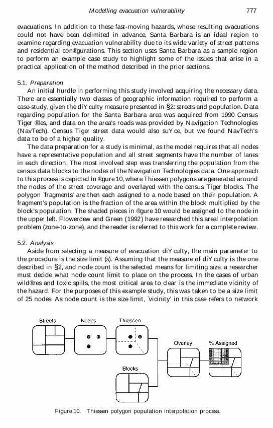
The data preparation for a study is minimal, as the model requires that all nodeshave a representative population and all street segments have the number of lanesin each direction. The most involved step was transferring the population from thecensus data blocks to the nodes of the Navigation Technologies data. One approachto this process is depicted in ® gure 10, where Thiessen polygons are generated aroundthe nodes of the street coverage and overlayed with the census Tiger blocks. Thepolygon fragments’ are then each assigned to a node based on their population. Afragment’s population is the fraction of the area within the block multiplied by theblock’s population. The shaded pieces in ® gure 10 would be assigned to the node inthe upper left. Flowerdew and Green (1992 ) have researched this areal interpolationproblem (zone-to-zone), and the reader is referred to this work for a complete review.

5.2. AnalysisAside from selecting a measure of evacuation diYculty, the main parameter to

the procedure is the size limit (s). Assuming that the measure of diYculty is the onedescribed in § 2, and node count is the selected means for limiting size, a researchermust decide what node count limit to place on the process. In the cases of urbanwild® res and toxic spills, the most critical area to clear is the immediate vicinity ofthe hazard. For the purposes of this example study, this was taken to be a size limitof 25 nodes. As node count is the size limit, vicinity’ in this case refers to network

Figure 10. Thiessen polygon population interpolation process.


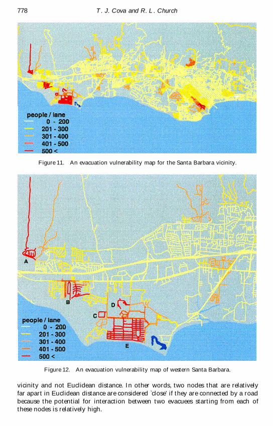
Figure 11. An evacuation vulnerability map for the Santa Barbara vicinity.

Figure 12. An evacuation vulnerability map of western Santa Barbara.

vicinity and not Euclidean distance. In other words, two nodes that are relativelyfar apart in Euclidean distance are considered close’ if they are connected by a roadbecause the potential for interaction between two evacuees starting from each ofthese nodes is relatively high.


Figure 11 shows the results of producing a complete map for the Santa Barbaravicinity. The thematic map unit is the number of people per lane in an road segment’sworst-case evacuation (i.e., maximum diYculty value less than 25 nodes).Conceptually, the map is a discrete surface de® ned only along the network. Becausenearby road segments are often in the same spatial evacuation vulnerability class,groups of segments organize themselves into perceivable vulnerability clusters. Wecall these clusters evacuation sheds, and they represent interesting areas for furtherinquiry. However, at this mapping scale the network is too dense to reveal whycertain neighbourhoods are highlighted.

Figure 12 shows a larger scale view of an area just west of the Santa BarbaraCity limits with many evacuation hot spots’. Communities (A) through (D) all havemore than 500 residents and only one exit lane. For this reason, there is greaterpotential for traYc congestion to impede an urgent evacuation of these neighbour-hoods. Despite the relatively large number of exits in the larger community (E), thepopulation density in this area is so high that the algorithm had no problem ® ndingnumerous potential evacuations where the number of residents per exit lane mightbe greater than 500.

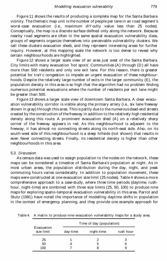
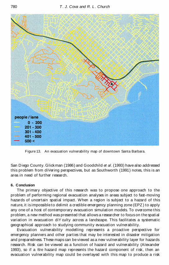
Figure 13 shows a larger scale view of downtown Santa Barbara. A clear evacu-ation vulnerability corridor is visible along the primary artery (i.e., six lane freewayshown in gray) through this area. This is partly due to the numerous dead-end streetscreated by the construction of the freeway in addition to the relatively high residentialdensity along this route. A prominent evacuation shed (A) on a relatively sharpcorner of the freeway appears in red. As this neighbourhood is adjacent to thefreeway, it has almost no connecting streets along its north-east side. Also, on itssouth-west side of this neighbourhood is a steep hillside (not shown) that results ineven fewer connecting streets. Finally, its residential density is higher than otherneighbourhoods in this area.

5.3. DiscussionAs census data was used to assign population to the nodes on the network, these

maps can be considered a timeslice of Santa Barbara’s population at night. As inmost urban areas, the population distribution during the day, night, and peakcommuting hours varies considerably. In addition to population movement, thesemaps were constructed at one evacuation size limit (25 nodes). Table 4 shows a morecomprehensive approach to a case-study, where three time periods (daytime, rush-hour, night-time) are combined with three size limits (25, 50, 100) to produce ninemaps for exploring spatio-temporal evacuation vulnerability in this area. Parrot andStutz (1991) have noted the importance of modelling daytime shifts in populationin the context of emergency planning, and they provide one example approach for

Table 4. A matrix to produce nine evacuation vulnerability maps for a study area.

Time of day (population)Evacuationsize limit day-time night-time rush hour

25 1 2 350 4 5 6

100 7 8 9


Figure 13. An evacuation vulnerability map of downtown Santa Barbara.

San Diego County. Glickman (1986 ) and Goodchild et al. (1993) have also addressedthis problem from diVering perspectives, but as Southworth (1991 ) notes, this is anarea in need of further research.

6. Conclusion

The primary objective of this research was to propose one approach to theproblem of performing regional evacuation analyses in areas subject to fast-movinghazards of uncertain spatial impact. When a region is subject to a hazard of thisnature, it is impossible to delimit a credible emergency planning zone (EPZ) to applyany one of a host of contemporary evacuation simulation models. To overcome thisproblem, a new method was presented that allows a researcher to focus on the spatialvariation in evacuation diYculty across a landscape. This facilitates a systematicgeographical approach to studying community evacuation vulnerability.

Evacuation vulnerability modelling represents a proactive perspective foremergency planners and other parties that may be interested in disaster mitigationand preparedness. These maps can be viewed as a new vulnerability layer for hazardsresearch. Risk can be viewed as a function of hazard and vulnerability (Alexander1993), so if a ® re hazard map represents the hazard component of risk, then anevacuation vulnerability map could be overlayed with this map to produce a risk


Figure 14. The potential role for evacuation vulnerability maps in risk mapping.

map. This opens the door to integrating evacuation vulnerability modelling with thenumerous GIS hazard models that have been developed. Figure 14 shows examplehazard layers and how they might be combined with an evacuation vulnerabilitylayer to explore issues of risk.

Another interesting area of research that needs to be addressed in this context isdeveloping new approaches to estimating the whereabouts of population in a cityat a relatively ® ne-grained level (e.g., census block) for ® xed points in time. Thisproblem is extremely complex, as population ¯ uctuations range from low-frequencyseasonal migrations to the noise’ of special events.

Also, there are also a host of interesting research questions and problems toaddress in developing new measures of evacuation diYculty and spatial evacuationvulnerability. First, this paper presented only one measure of evacuation diYculty,but there is a clear need to develop additional measures that take into considerationother factors that aVect evacuation diYculty (e.g., number of vehicles, special popula-tions) (Vogt and Sorensen 1992). These measures might be considered in the largerfamily of accessibility measures where they refer to the accessibility of a populationsubset out of a neighbourhood. Second, the modelling decision of how to limitevacuation size is an interesting area for further research. This paper presented ® veapproaches that may each have application in diVerent hazard or network contexts.An investigation into the strengths and weaknesses of these various approaches fordiVerent hazard and network contexts would be a valuable study.

Acknowledgments

The NCGIA is supported by the NSF through grant SBR 88± 10917. The authorswould like to thank Michael Goodchild for his general support and the followingpeople for their contribution to this project: Uwe Deichmann, Jonathan Gottsegen,Terry Figel, and the IJGIS reviewers. We also wish to thank Navigation Technologies(NavTech) for their generosity in allowing us access to their database for SantaBarbara County. An earlier version of this paper received the IGIF student paperaward at GIS/LIS 95, for which the lead author is especially grateful. The latterpart of this research was supported by an Eisenhower Graduate Fellowship fromthe National Highway Institute (NHI).


References

Alexander, D ., 1993, Natural Disasters (New York: Chapman and Hall ).Brainard J., Lovett A ., and Parfitt J., 1996, Assessing hazardous waste transport risks

using a GIS. International Journal of Geographical Information Systems, 10, 831± 849.Burke, L. M ., 1993, Race and environmental equity: a geographical analysis of Los Angeles.

Geo Info Systems, 3, 44± 50.Burrogh, P. A ., 1990, Methods of spatial analysis in GIS. International Journal of Geographical

Information Systems, 4, 221± 223.Carrara, A ., and Guzzetti, F. (editors), 1995, Geographical Information Systems in Assessing

Natural Hazards (Dordrecht: Kluwer Academic Publishers).Chou, Y. H ., 1992, Management of wild® res with a geographical information system.

International Journal of Geographical Information Systems, 6, 123± 140.Dangermond, J., 1985, Network allocation modelling for emergency planning. Proceedings

of the Conference on Emergency Planning: Emergency Planning, Simulation Series,Volume 15, Number 1, edited by J. M. Carroll (La Jolla: Society for ComputerSimulation), pp. 101± 106.

Dangermond, J., 1991, Applications of GIS to the international decade for natural hazardsreduction. In Proceedings of the Fourth International Conference on Seismic Zonation(Stanford University: Earthquake Engineering Research Institute) 3, pp. 445± 468.

de Silva, F., Pidd, M ., and Eglese, R ., 1993, Spatial decision support systems for emergencyplanning: an operational research/geographical information systems approach toevacuation planning. In Proceedings of the 1993 Simulation Multiconference on theInternational Emergency Management and Engineering Conference (San Diego: TheSociety for Computer Simulation), pp. 130± 133.

Dunn, C. E., 1992, Optimal routes in GIS and emergency planning applications. Area,24, 259± 267.

Emani, S., Ratick, S. J., Clarke, G . E., and Dow, K ., 1993, Assessing vulnerability to extremestorm events and sea-level rise using geographical information systems (GIS). InProceedings of GIS/L IS 93, (Bethesda, Maryland: American Society forPhotogrammetry and Remote Sensing), pp. 201± 209.

Emmi, P. C ., and Horton, C. A ., 1995, A Monte Carlo simulation of error propagation in aGIS-based assessment of seismic risk. International Journal of Geographical InformationSystems, 9, 447± 46.

Estes, J. E., McGuire, K . C., Fletcher, G . A ., and Foresman, T. W ., 1987, Coordinatinghazardous waste management activities using geographical information systems.International Journal of Geographical Information Systems, 1, 359± 386.

Evans, J. R ., and M inieka, E., 1992, Optimization algorithms for networks and graphs (NewYork: M. Dekker).

FEMA 1984, Application of the I-DY NEV system. Five demonstration case studies (Washington,DC: Federal Emergency Management Agency REP-8).

Flowerdew, R ., and Green, M ., 1992, Developments in areal interpolation methods andGIS. Annals of Regional Science, 26, 67± 78.

Fotheringham, A. S., and Rogerson, P. A ., 1993, GIS and spatial analytic problems.International Journal of Geographical Information Systems, 7, 3± 19.

Gatrell, A. C ., and Vincent, P ., 1991, Managing natural and technological hazards. InHandling Geographical Information: Methodology and Potential Applications. Edited byI. Masser and M. Blakemore (London: Longman), pp. 148± 180.

Glickman, T. S., 1986, A methodology for estimating time-of-day variations in the size of apopulation exposed to risk. Risk Analysis, 6, 317± 324.

Goodchild, M . F., 1987, A spatial analytic perspective on geographical information systems.International Journal of Geographical Information Systems, 1, 327± 334.

Goodchild, M . F., 1992, Geographical data modelling. Computers & Geosciences, 18,

401± 408.Goodchild, M . F., Klinkenberg, B., and Janelle, D . G ., 1993, A factorial model of aggregate

spatio-temporal behaviour: application to the diurnal cycle. Geographical Analysis,25, 277± 294.

Han, A ., 1990, TEVACS: Decision support system for evacuation planning in Taiwan. Journalof T ransportation Engineering-ASCE, 116, 821± 830.


Hobeika, A. G ., and Jamei, B., 1985, MASSVAC: a model for calculating evacuation timesunder natural disasters. Proceedings of the Conference on Emergency Planning,Emergency Planning, Simulation Series, Volume 15, Number 1, edited by J. M. Carroll(La Jolla: Society for Computer Simulation), pp. 23± 28.

Hobeika, A. G ., Radwan, A. E., and Jamei, B., 1985, T ransportation Actions to ReduceEvacuation T imes under Hurricane/Flood Conditions: A Case Study of V irginia BeachCity. Department of Civil Engineering, Virginia Polytechnic Institute and StateUniversity, Blacksburg, Virginia.

Hobeika, A. G ., K im, S., and Beckwith, R. E., 1994, A decision support system for developingevacuation plans around nuclear power stations. Interfaces, 24, 22± 35.

Hodgson, M . E., and Palm, R ., 1992, Attitude toward disaster: a GIS design for analysinghuman response to earthquake hazards. Geo Info Systems, July± August, 41± 51.

Honneycut, D ., 1996, Personal communication. Santa Barbara, California, December.Jin, L. M ., and Chan, S. P ., 1992, A genetic approach for network partitioning. International

Journal of Computer Mathematics, 42, 47± 60.Johnson, D . S., Aragon, C. R., McGeoch, L. A ., and Schevon, C ., 1989, Optimization by

simulated annealing: an experimental evaluation; part I, graph partitioning. OperationsResearch, 37, 865± 892.

Johnson, G . O ., 1992, GIS applications in emergency management, URISA Journal, 4, 66± 72.Kernighan, B. W ., and Lin, S., 1970, An eYcient heuristic procedure for partitioning graphs.

Bell Systems T echnical Journal, 49, 291± 307.Laguna, M ., Feo, T. A ., and Elrod, H . C ., 1994, A greedy randomized adaptive search

procedure for the two-partition problem. Operations Research, 42, 677± 687.McMaster, R. B., 1988, Modelling community vulnerability to hazardous materials using

geographic information systems. In Proceedings of the T hird Symposium on SpatialData Handling , pp. 143± 156. (Columbus: International Geographical Union).

Newsom, D . E., Madore, M . A ., and Jaske, R. T., 1992, Evacuation Modelling Near aChemical Stockpile Site. Argonne National Labs, Document ANL/CP-73412,Argonne, Illinois.

NRC 1980, Criteria for preparation, evaluation of radiological emergency response plans andpreparedness in support of nuclear power plants. U.S. Nuclear Regulatory Commission,NUREG-0654, Washington, D. C.

OFD 1992, T he Oakland tunnel ® re, October 20, 1991: a comprehensive report prepared by theOakland Fire Department. Oakland, California.

Parrot, R ., and Stutz, F. P ., 1991, Urban GIS applications. In Geographical InformationSystems, Volume 2: Applications, edited by D. J. Maguire, M. F. Goodchilld, D. W.Rhind, (London: Longman) 247± 260.

Perry, R ., 1985, Comprehensive Emergency Management: Evacuating T hreatened Populations(London: JAI Press, Inc.).

Pidd, M ., de Silva, F. N ., and Eglese, R. W ., 1996, A simulation model for emergencyevacuation. European Journal of Operations Research, 90, 413± 419.

Pirkul, H ., and Rolland, E., 1994, New heuristic solution procedures for the uniform graphpartitioning problem: extensions and evaluation. Computers and Operations Research,21, 895± 907.

Radke, J., 1995, Modelling urban/wildland interface ® re hazards within a geographicalinformation system. Geographic Information Sciences, 1, 9± 21.

Rejeski, D ., 1993, GIS and risk: a three culture problem. In Environmental Modelling withGIS, edited by M. F. Goodchild, B. O. Parks, and L. T. Steyaert, (New York: OxfordUniversity Press), pp. 318± 331.

Sheffi, Y., Mahmassani, H ., and Powell, W . B., 1982, A transportation network evacuationmodel. T ransportation Research A, 16A, 209± 218.

Shu-Quiang, W ., and Unwin, D . J., 1992, Modelling landslide distribution on loess soils inChina: an investigation. International Journal of Geographical Information Systems,6, 391± 405.

Sinuany-Stern, Z., and Stern, E., 1993, Simulating the evacuation of a small city: the eVectsof traYc factors. Socio-Economic Planning Sciences, 27, 97± 108.

Sorensen, J. H ., Carnes, S. A ., and Rogers, G . O ., 1992, An approach for deriving emergencyplanning zones for chemical munitions emergencies. Journal of Hazardous Materials,30, 223± 242.

Modelling evacuation vulnerability784

Sorensen, J. H ., Vogt, B. M ., and M ileti, D . S., 1987 Evacuation: an assessment of planningand research, Oak Ridge National Laboratory, ORNL-6376, Tennessee.

Southworth, F., 1991, Regional evacuation modelling: a state-of-the-art-review. Centre forTransportation Analysis, Oak Ridge National Laboratory, ORNL/TM-11740.

Southworth, F., and Chin, S. M ., 1987, Network evacuation modelling for ¯ ooding as aresult of dam failure. Environment and Planning A, 19, 1543± 1558.

Stone, J. R ., 1983, Hurricane Emergency Planning: Estimating Evacuation T imes for Non-metropolitan Coastal Communities, Sea Grant College Publication, UNC-SG-83± 2,North Carolina State University, Raleigh.

Tufekci, S., and K isko, T. M ., 1991, Regional evacuation modelling system (REMS): Adecision support system for emergency area evacuations. Computers & IndustrialEngineering, 21, 89± 93.

Urbanik, T. E., and Jamison, J. D ., 1992, State of the art in evacuation time estimate studiesfor nuclear power plants. NUREG/CR-4831, PNL-7776, U.S. Nuclear RegulatoryCommission, Washington, D.C.

Urbanik, T., Desrosiers, A., Lindell, M . K ., and Schuller, C. R ., 1980, Analysis oftechniques for estimating evacuation times for emergency planning zones. OYce ofNuclear Reactor Regulation, U.S. Nuclear Regulatory Commission, NUREG/

CR-1745, Washington, DC.Vogt, B. M ., and Sorensen, J. H ., 1992, Evacuation Research: A Reassessment. Oak Ridge

National Laboratory, ORNL/TM-11908, Tennessee.Wadge, G . 1988 The potential of GIS modelling of gravity ¯ ows and slope instabilities.

International Journal of Geographical Information Systems, 2, 143± 152.WSA (Wilbur Smith and Associates), 1974, Roadway Network and Evacuation Study, Seabrook,

New Hampshire, Report prepared for the Public Service Company of New Hampshire,New Haven, Connecticut, December.

Documents

Modelling community evacuation vulnerability …content.csbs.utah.edu/~cova/cova-church-1997.pdfint. j. geographical information science,1997,vol.11,no.8,763±784 Research Article