Modelling and Control of a Turbocharged

Burner Unit

Brian Solberg1, Palle Andersen2 and Jakob Stoustrup2

1Aalborg Industries A/S, Aalborg, Denmark, bso@es.aau.dk2Aalborg University, Aalborg, Denmark, {pa,jakob}@es.aau.dk

ABSTRACT: This paper concerns modelling and control of a novel turbochargedburner unit developed for small-scale industrial and marine boilers. The burnerconsists of a gas turbine mounted on a furnace. The burner has two inputs; oilflow to the gas generator (gas turbine combustion chamber) and oil flow to thefurnace, and two outputs; power and oxygen percentage in the exhaust gas. Thecontrol objective of the burner unit is to deliver the requested power set by e.g.an outer pressure loop while keeping a clean combustion and optimising efficiency.A first principle model is derived and validated against preliminary test data.The preliminary test shows that the model is capable of capturing the importantdynamics of the burner unit while more testing is required to determine the reasonfor discrepancies in gains. An analysis of the model shows that both dynamicsand gains change remarkably over the entire load range. However, local linearisedmodels of low order can be derived and used in a subsequent controller design.Also, the model includes an inverse response (non-minimum phase zero) fromthe gas generator oil flow to the controlled oxygen level. This means that whenchanging the oil flow to the gas generator, the oxygen level initially moves in theopposite direction before it moves in the long term direction. A control strategybased on a nonlinear feedforward and a linear feedback controller, adjusting theratio between the oil flow to the gas generator and to the furnace, is proposed.The feedforward is calculated from an inverse mapping of the requested poweroutput to find the two stationary oil flows while respecting oxygen constraints.Simulation results gathered from the developed nonlinear model with added noiseand external disturbances illustrate the efficiency of the proposed control strategy.

Keywords: turbocharger, gas turbine, first principle modelling, lumped parametermodels, burner control

1 INTRODUCTION

Most burners, shipped with industrialand marine boilers today, are equippedwith a fan to supply the combustionwith air. Such fans consume considerableamounts of electric power and producenoise. Further, to achieve a high turn-down ratio using a conventional burner,more than one atomiser is needed. Theburner considered in this paper is a twostage burner in which the first stage drives

a gas turbine and the second stage is aconventional furnace burner. This concepthas multiple advantages over the afore-mentioned fan concept. First of all burnerefficiency is high as there is no longer aneed for electrical fan actuation. Further,the turndown ratio is increased in the waythat the gas turbine can operate alone(however, this operation mode is not verythermodynamically efficient). Finally, thegas turbine concept increases the gas ve-

locity through the boiler convection partwhich leads to a higher heat transfer tothe metal.

However, this new burner concept re-quires a more comprehensive control strat-egy than the conventional burners to max-imise efficiency and keep a clean combus-tion to e.g. minimise the amount of pollu-tant expelled from the funnel. This factoris especially important when the burner isinstalled on ship boilers as large penaltiesare assigned to shipowners if the smokecoming out of the stacks is too harmfulto the environment.

The control problem is complicated bythe high degree of nonlinearities in the sys-tem and further, the process exhibits aninverse response from the gas generator(gas turbine combustion chamber) fuel in-jection to the flue gas oxygen level which isused as a parameter for clean combustion.

In relation to the automotive indus-try many people have addressed modellingand control of turbocharged diesel engines– see e.g. [1, 2, 3, 4]. From these works,results on the turbocharger modelling canbe used. There is obviously a resemblancebetween the setup presented in this pa-per and the gas turbine found on powerplants and combined cycle power plants.A model of a stationary gas turbine canbe found in [5].

We derive a model based on first prin-ciples rather than using system identifi-cation techniques to specify a black boxmodel based on e.g. linear parametricmodels. This technique is adopted as thesemodels tend to be valid over a wider oper-ating range. The goal is to derive a lumpedparameter model that reflects the burnerdynamics as well as possible from knowl-edge of the system behaviour and mea-surement. This approach is also taken toachieve insight to the burner process. Fur-ther, a detailed model like this will be ofgreat value as a simulation platform forcontroller designs. Model verification ex-periments have been performed at AalborgIndustries’ (AI) test centre.

Regarding controller design, principlessuch as traditional selector and ratio con-trol of burners can be used – see e.g.[6]. However, many other methods ex-

ist and especially model predictive control(MPC) [7, 8, 9] is an interesting candidateas it can naturally handle constraints oninputs and state variables. However, inthis paper we focus on the control proper-ties of the burner unit and therefore stickwith traditional selector and ratio controlwith a nonlinear feedforward from setpointchanges.

We show that even though the process isnonlinear and includes inverse responses, asimple ratio controller can control the pro-cess. However, if more advanced controlmethods are to be used it is expected tobe necessary to handle the nonlinearitiesin the control setup.

The paper is organised as follows: Firsta short system description is given andassumptions made for modelling purposesare presented. Leading is the modelderivation followed by a discussion of thecontrol properties. Subsequently the con-trol strategy is described, simulation re-sults presented and conclusions and futurework are discussed.

2 SYSTEM DESCRIPTION

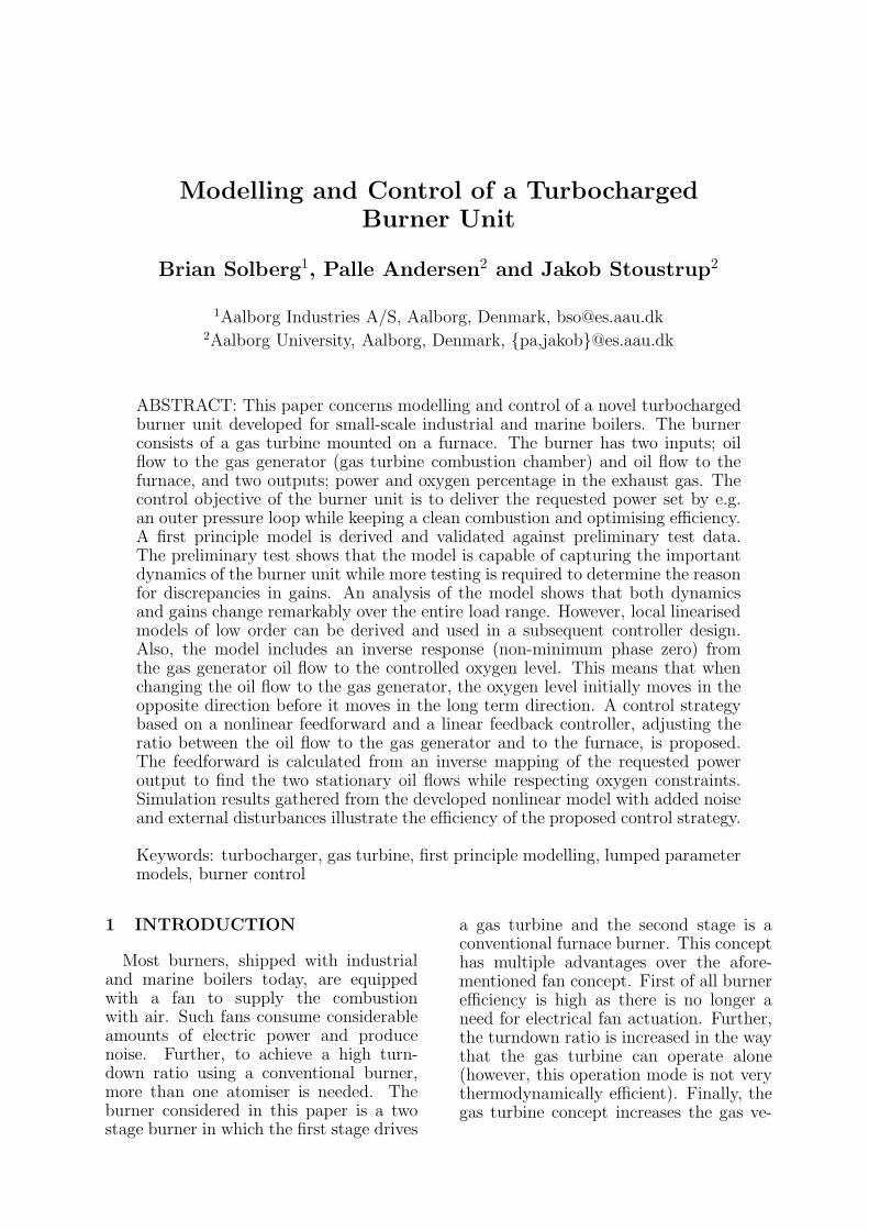
A sketch of the burner unit is shownin Figure 1, and the functionality is ex-plained below.

The units c, t and gg comprise thegas turbine. Fuel, fu1, is injected andburned in the gas generator, gg, and thehot gas leaving the combustion drives theturbine, t, which rotates the shaft of theturbocharger delivering power to drive thecompression process in the compressor, c.Air is sucked in at the compressor inlet,and the hot combustion flue gas leavesthe turbine to enter the second combus-tion chamber, the furnace, fn. Here fuelis added again, fu2, and another combus-tion takes place. More than 70% of thetotal fuel flow is injected into the furnace.The hot flue gas leaves the furnace and en-ters the boiler convection part before leav-ing through the funnel.

Before proceeding to the model deriva-tion we set up some general assumptionsto simplify the modelling process. Theseassumptions are listed and explained be-low.

����������������������

shaft

gg

ct

fn

fu1

fu2

a

Figure 1: Drawing of the turbochargedburner system. c is the compressor, t isthe turbine, gg is the gas generator (thefirst combustion chamber) and fn is thefurnace (the second combustion chamber).a is the fresh air inlet, and fu1 and fu2are the fuel inputs.

Assumption 2.1. The ambient pressureis constant.

The pressure in the engine room ona ship may vary. This will influencethe pressure ratio across the compres-sor as inlet air is taken from the engineroom. However, the setup concerned inthis project is situated on shore in a testcentre where ventilation is expected tocause negligible pressure variations.

Assumption 2.2. The metal part sepa-rating the flue gas and the water-steampart consists of one piece of metal with thesame temperature.

This assumption is justified by the factthat most boilers include a pressure con-trol loop keeping the pressure around aconstant reference value, e.g. 8 bar, mean-ing that temperature variations are small.

Assumption 2.3. All energy losses in thesystem leave through the funnel.

This assumption is made because lossesin terms of heat are negligible comparedto the total amount of energy supplied tothe system. A rough estimate of the rel-ative heat losses was shown in [10] to be< 0.0002 per thousand. Furthermore, no

friction losses from the shaft of the tur-bocharger are considered.

Assumption 2.4. The pressure in thefurnace is equal to the ambient pressure.

Measurement performed over the con-vection part of the test boiler showed apressure loss of about 9000 Pa which issmall compared to the range of operation.The ambient pressure assumption is in-cluded to have consistency in the model;no fuel and air flow ⇒ no flue gas flow.

Assumption 2.5. The conditions in thecontrol volumes are homogeneous.

This assumption reflects the earlierstatement that we are constructing alumped parameter model. Furthermore,we will use a backwards place discreti-sation. The reason for this is that us-ing for instance a bilinear place discreti-sation method introduces unwanted righthalf plane zeros in a linear model [11].

Assumption 2.6. The specific heat ca-pacity, cp,f , and molar mass, Mf , of theflue gas throughout the process are as-sumed to be constant.

An analysis of the flue gas carried outin [11] justifies this assumption. In generalwe do not know Mf . To find this we wouldhave to make use of both a mass balanceand a mole balance to find Mf = m

n. How-

ever, as the analysis of the flue gas in [11]shows; the molar mass of the flue gas evenafter as stoichiometric combustion is ap-proximately equal to that of atmosphericair. Therefore, we assume a constant mo-lar mass of the flue gas.

Assumption 2.7. The flue gas can beviewed as an ideal gas.

The reference level for the enthalpy isset to T0 = 273.15 K or 0 ◦C, however, alltemperatures are kept in kelvin (T [K]).The reason for this choice is that manyof the specific heat capacity data are onlyavailable from 0 ◦C and up.

2.1 ModellingThe modelling is divided into two main

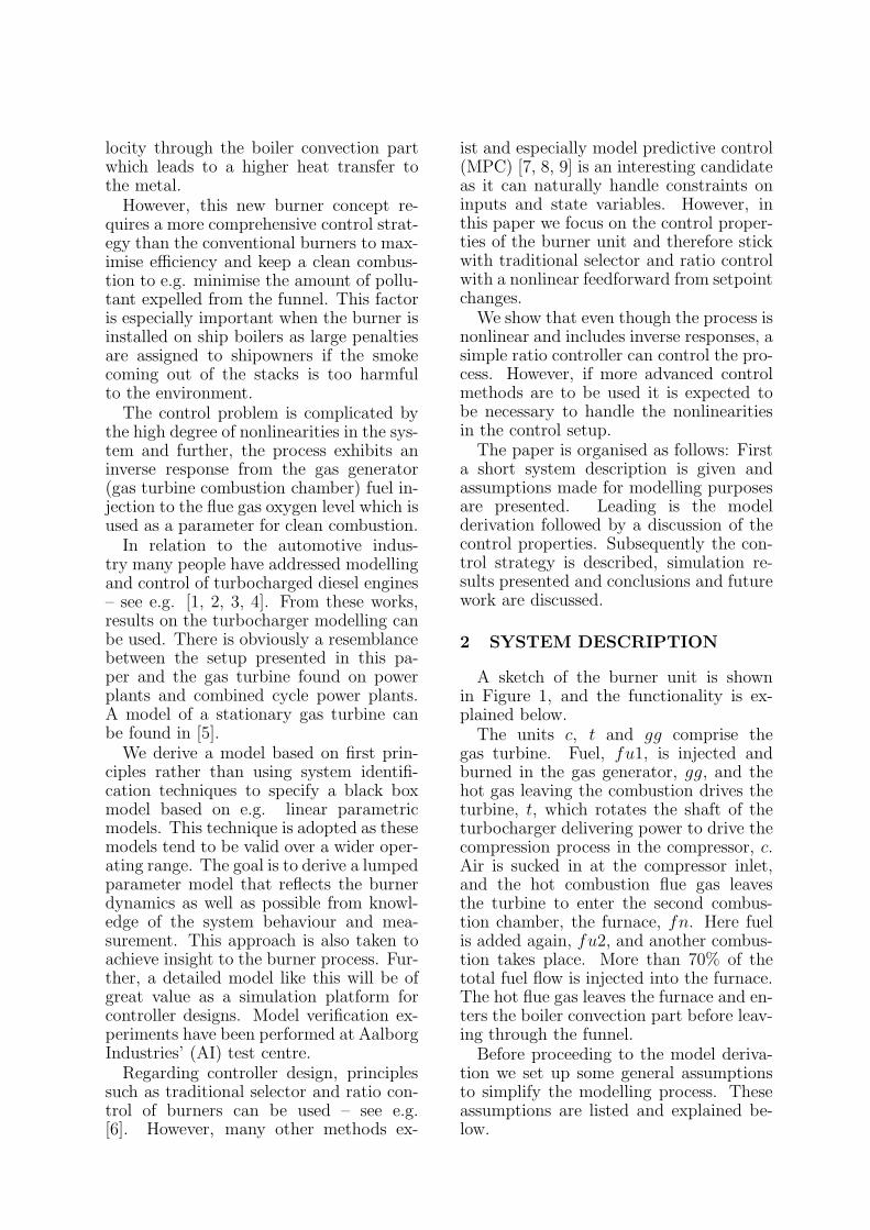
sections: one dealing with the thermody-namic properties of the gas turbine andfurnace system and another dealing withthe oxygen balance. In Figure 2 the gasturbine is presented in a schematic dia-gram useful for modelling purposes. At-tempts have been made to include the fourducts indicated on the figure in the model.This was done by using Euler equations in-cluding friction losses. However, the resultof modelling these ducts did not contributeto the validity of the resulting model andwill be omitted here.

Turbine

Compressor

Shaft

Air

Flue gas

Duct 1 Duct 2

Duct 3Duct 4

Gas generatorFuel

Figure 2: Schematic diagram showing theinterconnection of the components thatmake up the gas turbine.

2.2 Turbocharger ModelThere exists a lot of literature con-

cerning mean values modelling of tur-bocharged engines. The results from thiscan be applied to this burner unit. Fur-thermore, the book [12] provides a goodreference on turbo machinery.

Most of the modelling in this section isbased on results from [3, 13, 4, 2]. As men-tioned above, heat losses are neglected,and it is assumed that the processes in thecompressor and turbine can be viewed asadiabatic reversible compression and ex-pansion respectively. Such processes arecalled isentropic and have the followingproperties useful for the model derivation:

2.2.1 Properties of isentropic processesFor an ideal gas undergoing an isen-

tropic process, the following relationshipis valid [14]:

(Tois

Ti

)

=

(po

pi

)γ−1

γ

(1)

where Ti is the inlet temperature of theworking fluid, Tois

is the outlet tempera-ture under isentropic conditions. pi andpo are the inlet and outlet pressure respec-tively and the adiabatic index γ = cp

cv=

cp

cp−R

Mf

where R = Mf(cp − cv) also known

as the ideal gas constant.

2.2.2 Compressor modelTo account for the compressor not being

ideal in reality, we introduce the compres-sor isentropic efficiency 0 ≤ ηc ≤ 1 as theratio between theoretical isentropic tem-perature rise and actual temperature rise,[14]:

ηc =Tois,c − Ti,c

To,c − Ti,c

(2)

Equations (1) and (2) can be combined tofind an expression for the temperature atthe compressor outlet:

To,c = Ti,c

(

1 +1

ηc

[(po,c

pi,c

) γ−1

γ

− 1

])

(3)A common assumption when working withcompressor and turbine units is to regardthem as steady state steady flow processes(SSSF). The mass in the compressor andturbine is relative low compared to themass flow rate due to the small compres-sor and turbine volume. Hence mass, tem-perature and pressure are all assumed tochange instantly with changing inlet con-ditions rendering the dynamics negligible.

This means that the mass balance forthe compressor is given as:

0 =dmc

dt= mi,c − mo,c (4)

Furthermore, the energy balance can bewritten as:

0 =d(mccp,f(To,c − T0) − pcVc)

dt(5)

= mi,ccp,f(Ti,c − T0)+

− mo,ccp,f(To,c − T0) + Pc

where Pc is the power delivered from theshaft to the compressor, which, usingEquations (4) and (5) can be expressed as:

Pc = mccp,f(To,c − Ti,c) (6)

where mc = mi,c = mo,c. Now inserting(3) into this expression gives:

Pc = mccp,fTi,c

1

ηc

[(po,c

pi,c

)γ−1

γ

− 1

]

(7)

2.2.3 Turbine modelThe turbine in the turbocharger is a

fixed geometry turbine (FGT). As in caseof the compressor we start by introducingthe turbine isentropic efficiency 0 ≤ ηt ≤ 1as the ratio between actual temperaturedrop and theoretical isentropic tempera-ture drop, [14]:

ηt =Ti,t − To,t

Ti,t − Tois,t

(8)

Using Equations (1) and (8) an expressionfor the temperature at the turbine outletcan be found:

To,t = Ti,t

(

1 − ηt

[

1 −(

po,t

pi,t

)γ−1

γ

])

(9)The mass and energy balances for the tur-bine are equivalent to those of the com-pressor, except that the work done by theturbine is positive so that energy is trans-ferred from the turbine by means of work.This means that we can find an expressionfor the power absorbed in the shaft fromthe turbine:

Pt = mtcp,f(Ti,t − To,t) (10)

where mt = mi,t = mo,t. Inserting (9) weget:

Pt = mtcp,fTi,tηt

[

1 −(

po,t

pi,t

) γ−1

γ

]

(11)

2.2.4 Shaft modelThe model of the shaft connecting the

compressor and turbine has the purposeof describing the turbocharger speed, ω.This can be done by considering the en-ergy balance for the shaft. The kinetic en-ergy for the shaft is:

Ukin =1

2Iω2 (12)

where I is the inertia of the rotating parts.Hence the energy balance is given as:

Iωdω

dt= ηmPt − Pc − Pf (13)

where Pf is a friction term, which is as-sumed to be negligible compared to thepower delivered by the turbine and thepower it takes to drive the compressor.Furthermore, the mechanical efficiency,ηm, is set to 1 below. So inserting the com-pressor and turbine power terms from (7)and (11), the model for the shaft becomes:

1︸︷︷︸

f33

dω

dt=

0

B

B

B

B

B

B

@

mtcp,fTi,tηt

2

41−

„

po,tpi,t

«γ−1

γ

3

5−

mccp,fTi,c1ηc

2

4

„

po,cpi,c

«γ−1

γ−1

3

5

1

C

C

C

C

C

C

A

/(Iω)

︸ ︷︷ ︸

h3

(14)

This is the equation governing the tur-bocharger dynamics.

2.2.5 Turbocharger data sheetsWe still need to find expressions for the

flow through the compressor and turbineas well as expressions for the efficiency ofthese components. An overview of differ-ent methods for deriving such can be foundin [3]. Some are partly based on first prin-ciple and others are functions derived fromcurve fitting techniques. The parametersin both approaches are estimated from tur-bine and compressor maps. These can beacquired from the turbocharger manufac-turer.

Usually the flow and speed data arescaled to make the maps independent ofthe inlet conditions (pi, Ti). The scaling isdone according to:

˙m =m√

Ti

pi

[kgs

√K

MPa

]

, N =ω

2π√

Ti

[1

s√

K

]

(15)

where N is scaled rotations per second.The dependency of the speed and pres-sure ratios on the flow and efficiency ofthe compressor and turbine are:[mc

ηc

]

= gc

(

ω,po,c

pi,c

)

,

[mt

ηt

]

= gt

(

ω,po,t

pi,t

)

(16)

As discussed in [3], it is not always easyto find a function gc, for the compressormap, having flow as output. An alterna-tive mapping for the compressor is possible[3]:

[po,c

pi,c

ηc

]

= g′

c (ω, mc) (17)

Knowledge of the flow can be gained by in-troducing a control volume correspondingto the manifold connecting the compres-sor and the gas generator. Using the one-dimensional momentum balance for thiscontrol volume gives:

pgg − po,c

ρc

+ gz cos(θ) +dvc

dtz = −ht(vc)

(18)The compressor mass flow can be foundas mc = ρcAvc, where A is the diame-ter of the pipe. This corresponds to us-ing ”Model II” in [3] . This approach hasthe advantages of allowing for modellingof the pressure drop over the gas genera-tor inlet duct. However, as described in[3] the new differential equation increasesmodel stiffness.

In this work we will use the mappingsshown in (16). The data available for theturbocharger used are limited. For thisreason we use a method for approximat-ing the mappings gc and gt which is partlybased on physical insight instead of e.g.parameterising the data by using regres-sion to fit some polynomial model or traina neural network model. The advantage ofthis is that the extrapolation of data tendsto give better predictions.

2.2.6 CompressorThe method used to describe the com-

pressor flow and efficiency is described in[1]. This is the method investigated in[3] performing the best when the outputis flow and efficiency. Whereas the neu-ral network approach seems to be superiorfor the alternative model, in [10] the prob-lems using a neural network model for thecompressor unit under consideration wasillustrated.

Expressing the enthalpy for the gas un-dergoing the compression as hi,c = cp,fTi,c

and ho,c = cp,fTo,c for the inlet and outlet

respectively, we can write Equation (6) as:

Pc = mc(ho,c − hi,c) = mc∆hc (19)

Using Equation (7) we find the followingrelation between the enthalpy change andthe pressure ratio over the compressor:

∆hc = cp,fTi,c

1

ηc

[(po,c

pi,c

) γ−1

γ

− 1

]

(20)

Looking at the ideal case ηc = 1, ∆hc,ideal

can be estimated from Euler’s equation forturbomachinery. For this purpose we con-sider a compressor with radially inclinedimpeller blades, no pre-whirl and no back-sweep [14, p. 372-375]:

∆hc,ideal = UoCwo − UiCwi (21)

where Uo is the blade speed at the im-peller tip, Cwo, is the tangential compo-nent of the gas velocity (whirl) leaving theimpeller, Ui is the velocity of the impellerat the impeller entry and Cwi is the tan-gential component of the gas velocity en-tering the impeller. However, as we haveassumed no pre-whirl Cwi = 0 and hence

∆hc,ideal = UoCwo = UcCc (22)

In practice, the whirl velocity Cc is differ-ent from the ideal Cc,ideal = Uc due to in-ertia of air trapped between blades. Thisis known as slip, and

σ =Cc

Uc

(23)

is known as the slip factor. Hence:

∆hc,ideal = σU2c (24)

The slip factor is dependent on the massflow rate through the compressor, mean-ing that the compressor pressure ratio isa function of both turbocharger speed andmass flow. The ratio between the ideal andactual enthalpy changes across the com-pressor is the compressor efficiency.

ηc =∆hc,ideal

∆hc

(25)

Using Equation (20) we have:

∆hc,ideal = cp,fTi,c

[(po,c

pi,c

) γ−1

γ

− 1

]

(26)

[1] uses these physical considerations withsome empirical assumptions to derive amodel for the efficiency and mass flow.They first define the dimensionless param-eter Ψ, also known as the temperature co-efficient or the blade loading coefficient,which is closely related to the slip factor(and the inverse square of the blade speedratio as defined later for the turbine), as:

Ψ =cp,fTi,c

[(po,c

pi,c

γ−1

γ − 1)]

12U2

c

(27)

where Uc = 12Dcω. The normalised com-

pressor flow rate, Φ, or flow coefficient isdefined as:

Φ =mc

ρaπ4D2

cUc

(28)

and the inlet Mach number M is:

M =Uc

√

γ RMf

Ti,c

(29)

The normalised flow and the compressorefficiency are assumed to be functions ofΨ and M :

Φ =k3Ψ − k1

k2 + Ψ, ki = ki1 + k12M (30)

ηc = a1Φ2 + a2Φ + a3, ai =

ai1 + ai2M

ai3 − M(31)

for i = 1, 2, 3. And now

mc = Φρa

π

4D2

cUc (32)

The method described in [2], based onphysical insight as well, was also investi-gated. This method proposes a parametri-sation of the enthalpy in (26) using theblade speed and the mass flow. However,the method seems not to be applicable forthe compressor at hand and gives a poorerfit than the method described above.

2.2.7 TurbineEuler’s equations can also be used for

the turbine, noting that by assuming noswirl at the turbine outlet the tangentialcomponent of the gas velocity at the outletbecomes zero, Cwt = 0. The rest of theequations follow the same lines as for thecompressor.

However, for the turbine we use a dif-ferent method for modelling flow and ef-ficiency. Following [3] we model the flowthrough the turbine as the flow throughnozzles (or diffusers). The well known flowequations are [12, p. 449-451]

mt = At

pi,t√

Ti,tR

√2γ

γ − 1

[

Π2γ − Π

γ+1

γ

]

(33)where

Π = max(Πt, Πcrit) = max(po,t

pi,t

, Πcrit)

(34)Here the critical pressure ratio is: Πcrit =

2γ+1

γγ−1 . At is the effective flow area. This

is assumed to be a function of the tur-bocharger speed and the pressure ratioover the turbine given as:

At(N ,po,t

pi,t

) = (35)

a2(N)

(po,t

pi,t

)2

+ a1(N)po,t

pi,t

+ a0(N)

where

ai(N) = a2iN2 + a1iN + a0i (36)

this form is not standard but found to bea better fit than the suggestion in [3].

According to [3] the efficiency can bemodelled as a function of the blade speedratio:

Ut

Ct

=12Dtω

√

2cpTi,t

(

1 −(

po,t

pi,t

) γ−1

γ

)(37)

where Ut is the velocity of the blade speedat the point where the flow enters, and Ct

is the tangential component of the air ve-locity at the entry to the turbine rotor.The efficiency is then parameterised as:

ηt = b2(N)

(Ut

Ct

)2

+ b1(N)Ut

Ct

+ b0(N)

(38)where

bi(N) = b1iN + b0i (39)

2.3 Gas Generator Combustion ModelIn this paragraph a model used for the

combustion taking place in the gas gen-erator is described. The idea is to calcu-late the adiabatic flame temperature. Theapproach taken is to construct an artifi-cial infinitesimal combustion control vol-ume. The mass balance for such a controlvolume is given as:

mcb,gg = mc + mfu1 (40)

here mc and mfu1 is the air flow and fuelsupplied to the combustion, and mcb,gg isthe mass flow of the flue gas leaving thecombustion. Likewise the energy balanceis given as:

mcb,gghcb,gg = mchc + mfu1(hfu + Hfu)(41)

where hc, hfu1 and hcb,gg are the specificenthalpies of the inflowing and outflowingfluids, and Hfu is the calorific value for thefuel. Rearranging to isolate hcb,gg gives:

hcb,gg =mchc + mfu1(hfu + Hfu)

mcb,gg

(42)

Inserting h = cp,f(T − T0) gives:

Tcb,gg =

(

mccp,f(Tc − T0)+mfu1(cp,fu(Tfu − T0) + Hfu)

)/

(mcb,ggcp,f) + T0 (43)

2.4 Gas Generator ModelThe gas generator is treated as one con-

trol volume. The mass balance for the gasgenerator is given as:

dmgg

dt= Vgg

dρgg

dt=mi,gg − mo,gg

=mcb,gg − mt (44)

where Vgg is the volume of the gas gener-ator and ρgg is the density of the flue gasin the gas generator. mgg is the mass offlue gas in the volume which can be ex-pressed in terms of temperature and pres-sure through the ideal gas equation:

mgg = Vggρgg, ρgg =pggMf

RTgg

(45)

where Tgg is the temperature in the gasgenerator and pgg is the pressure. Thederivative of ρgg is:

dρgg

dt=

(Mf

RTgg

)dpgg

dt−(

pggMf

RT 2gg

)dTgg

dt

=ρgg

pgg

dpgg

dt− ρgg

Tgg

dTgg

dt(46a)

Substituting into (44) gives:

1

pgg︸︷︷︸

f11

dpgg

dt− 1

Tgg︸ ︷︷ ︸

f12

dTgg

dt=

mcb,gg − mt

mgg︸ ︷︷ ︸

h1

(47)

The energy balance for the gas generatoris given as:

d[mggcp,f(Tgg − T0) − pggVgg]

dt= (48)

mcb,ggcp,f(Tcb,gg − T0) − mtcp,f(Tgg − T0)

Note that we have not included any en-ergy transfer to or storage in the metalconstruction as these contributions are as-sumed to be small. Expanding the deriva-tive gives:

cp,f(Tgg − T0)dmgg

dt+ (49)

+ mggcp,f

dTgg

dt− Vgg

dpgg

dt=

mcb,ggcp,f(Tcb,gg − T0) − mtcp,f(Tgg − T0)

Now dmgg

dtfrom (44) can be substituted

into (49) and by rearranging we arrive at:

−Vgg︸ ︷︷ ︸

f21

dpgg

dt+ mggcp,f︸ ︷︷ ︸

f22

dTgg

dt= (50)

mcb,ggcp,f(Tcb,gg − Tgg)︸ ︷︷ ︸

h2

The differential equations (14), (47) and(50) constitute the model of the gas tur-bine. Note that there will be a pressuredrop across the gas generator which hasnot been included in the model.

2.5 Furnace Combustion ModelThe furnace combustion model is iden-

tical to the combustion model for thegas generator described previously with achange of variables. Hence the flue gasflow and temperature from the combustionand for the furnace can be written as:

mcb,fn = mt + mfu2 (51)

and

Tcb,fn =

(mtcp,f(Tt − T0)+

mfu2(cp,fu(Tfu − T0) + Hfu)

)/

(mcb,fncp,f) + T0 (52)

respectively.

2.6 Furnace ModelThe furnace model is supposed to cap-

ture the temperature dynamics in the fur-nace. Such a model might be dividedinto multiple control volumes includingthe convection tubes to achieve a more ac-curate model. However, here we focus onea single control volume. The mass balanceis:

dmfn

dt= mcb,fn − mfn (53)

Where mfn is the flue gas flow leavingthrough the funnel. As the pressure in thefurnace is regarded as constant, pfn = pa,the energy balance becomes:

[dmfncp,f(Tfn − T0)]

dt= −Q+ (54)

mcb,fncp,f(Tcb,fn − T0) − mfncp,f(Tfn − T0)

where Tfn is the furnace temperature and

Q = αc,fn(Tfn − Tm) is the energy trans-ferred to the metal wall of the furnace andconvection part with Tm being the temper-ature of the wall and αc,fn being the heattransfer coefficient. Expanding the deriva-tives using (53) and rearranging gives:

1︸︷︷︸

f44

dTfn

dt=

mcb,fncp,f(Tcb,fn − Tfn) − Q

mfncp,f︸ ︷︷ ︸

h4

(55)

where mfn is found from:

mfn = ρfnVfn =pfnMf

RTfn

Vfn (56)

where Vfn is the volume of the furnace.Before finding the output mass flow,

mfn, the change in density, ρfn, of the fluegas must be found. Such derivations areequivalent to those in (46) and as the pres-sure is constant, the first term in (46a) iszero leaving the following equation for thechange in density:

dρfn

dt= −ρfn

Tfn

dTfn

dt(57)

which together with (53) and (55) givesthe mass flow:

mfn =mcb,fncp,f(Tcb,fn + T0) − Q

(Tfn + T0)cp,f

(58)

2.7 Oxygen ModelThe oxygen model is divided into two;

one describing the oxygen fraction, xgg,O2,

in the gas generator and another describ-ing the oxygen fraction, xfn,O2

, in the fur-nace. These models do not treat the com-bustion meaning that the inputs to thesemodels are the outputs from the com-bustion. However, the two models arevery similar and will be treated in general.First we put up the mole balance for thecontrol volume:

dn

dt= ni − no (59)

where ni and no are the mole flows enter-ing and leaving the container respectivelyand n is the number of moles accumulated.Now the mole balance for the oxygen canbe expressed as:

d(nxo,O2)

dt= nixi,O2

− noxo,O2(60)

using a backward difference place discreti-sation, differentiating gives:

ndxo,O2

dt+ xo,O2

dn

dt= nixi,O2

− noxo,O2

(61)

Substituting (59) into this expression andrearranging gives:

dxo,O2

dt=

1

τ(xi,O2

− xo,O2) (62)

where, the time constant is τ = nni

. Re-member also that we can find n as n =pV

RT= m

Mf. Using the fact that Mf for the

flue gas is assumed constant gives the timeconstant as τ = m

mi. For the gas generator

and furnace the equations are:

1︸︷︷︸

f55

dxgg,O2

dt=

1

τgg

(xcb1,O2− xgg,O2

)

︸ ︷︷ ︸

h5

(63)

and

1︸︷︷︸

f66

dxfn,O2

dt=

1

τfn

(xcb2,O2− xfn,O2

)

︸ ︷︷ ︸

h6

(64)respectively.

As is apparent from these equations weneed to know both, ni and xi,O2

to makeuse of the differential equation. These aredetermined by studying the combustiontaking place.

2.7.1 Combustion in gas generatorThe combustion is assumed to be com-

plete. A complete combustion is a processwhich burns all the carbon C to CO2, allthe hydrogen H to H2O and all sulfur Sto SO2. If there are any unburned compo-nents in the exhaust gas such as C, H2 andCO the combustion process is incomplete.The mole flows of carbon and hydrogencoming in with the fuel are:

nC1 =mfu1yC

MC

, nH1 =mfu1yH

MH

(65)

where yC and yH are the mass fractions ofcarbon and hydrogen in the fuel. We as-sume here that yH = 1−yC hence ignoringsulphur and other purely represented com-ponents in diesel and heavy fuel used formarine boilers.

We assume that the atmospheric air forthe combustion consists of 21% O2 and79% N2, here the percentages represent

mole percentage and we denote the oxy-gen fraction as xO2,atm. Next the reactionschemes for the process are laid down tobe able to determine how much oxygen isleft in the flue gas after combustion andwhat the different compounds in the fluegas are. Reaction schemes:

nCC + nCO2 −→ nCCO2 (66)

nHH +1

4nHO2 −→

1

2nHH2O (67)

Hence the mole flow of oxygen leaving thecombustion is:

ncb1,O2= nc,O2

− (nC1 +1

4nH1) (68)

where nc,O2= ncxO2,atm with nc = mc

Mair=

mc

Mf. We also have nN2,c = nc(1 − xO2,atm).

Finally, the total amount of moles leavingthe combustion is given as:

ncb1 = ncb,O2+ nN2

+ nC +1

2nH (69)

This equation works only for combustionwith atmospheric air as is the case in thegas generator. The reason is that we donot keep track of the components in theflue gas during the rest of the process.However, we notice that, as we have as-sumed that Mf is constant, we can findthe total amount of mole leaving the com-bustion as ncb1 =

mc+mfu1

Mf. The expres-

sion for the oxygen fraction entering thegas generator then becomes:

xcb1,O2=

ncb1,O2

ncb1=

mcb1,O2

mcb1

(Mf

MO2

)

(70)

Now in the mean time the last bracketon the right hand side of Equation (70)is close to unity (Mf/MO2

≈ 0.9). Hencean approximate solution could be obtainedby treating the mole and mass fraction asequal.

2.7.2 Combustion in furnaceThe derivation of the expression for the

oxygen fraction of the flue gas leaving thefurnace combustion is identical to that ofthe gas generator combustion due to theassumption of constant molar mass of the

flue gas. The combustion air is the flue gasleaving the turbine having the oxygen frac-tion xgg,O2

. The oxygen fraction is givenas:

xcb2,O2=

ncb2,O2

ncb2

(71)

2.7.3 FuelIn relation to combustion we need to

know what fuel we are using to find outthe ratio between carbon and hydrogen. Incase of heavy fuel, one can order an anal-ysis of the fuel to obtain such data. Incase of diesel we assume that we know thestructure of the main molecule. Assumingthat it consists only of carbon and hydro-gen atoms the general molecule looks like:

Diesel : CXHY (72)

The mole fraction of carbon and hydrogenin the diesel can be found as:

xC =X

X + Y, xH = 1 − xC =

Y

X + Y(73)

From this we can find the average molarmass of diesel as:

Mfu = xCMC + xHMH (74)

and so the mass fractions of carbon andhydrogen are:

yC = xC

MC

Mfu

, yH = xH

MH

Mfu

(75)

In this work we assume X = 15 and H =32.

2.8 Model SummaryThe total model is best presented in de-

scriptor form as:

F (x)dx

dt= h(x, u, d) (76a)

y = g(x, u, d) (76b)

where x = [pgg, Tgg, ω, Tfn, xgg,O2, xfn,O2

]T ,u = [mfu1, mfu2]

T , d = [Ta, Tfu, Tm]T , and

y = [mfu, Q, xfn,O2]T , mfu = mfu1 + mfu2.

Expanding, (76a) has the form:

f11 f12 0 0 0 0f21 f22 0 0 0 00 0 f33 0 0 00 0 0 f44 0 00 0 0 0 f55 00 0 0 0 0 f66

dpggdt

dTgg

dtdωdt

dTfndt

dxgg,O2dt

dxfn,O2dt

=

h1

h2

h3

h4

h5

h6

(77)

where the elements fij and hi were indi-cated in the model derivation in Equations(14), (47), (50), (55), (63) and (64).

F is never singular, hence it has a welldefined inverse, so (76a) can be writtenas an ordinary differential equation: x =f(x, u, d) = F−1(x)h(x, u, d).

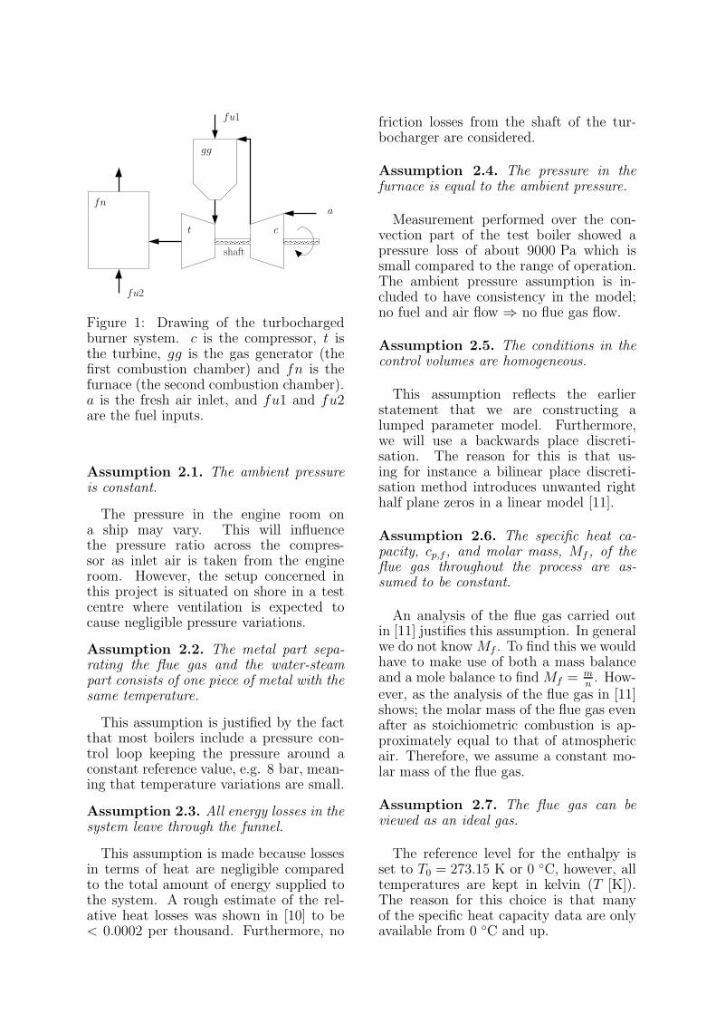
2.9 Model VerificationPreliminary test data have been col-

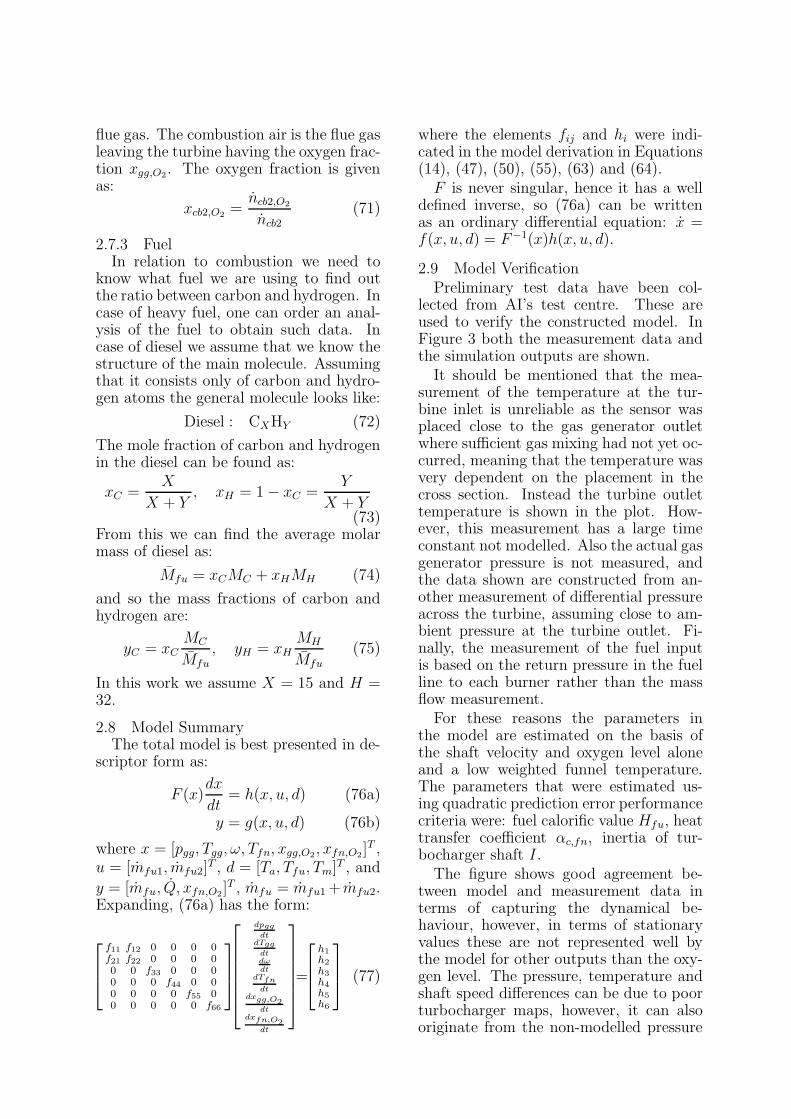
lected from AI’s test centre. These areused to verify the constructed model. InFigure 3 both the measurement data andthe simulation outputs are shown.

It should be mentioned that the mea-surement of the temperature at the tur-bine inlet is unreliable as the sensor wasplaced close to the gas generator outletwhere sufficient gas mixing had not yet oc-curred, meaning that the temperature wasvery dependent on the placement in thecross section. Instead the turbine outlettemperature is shown in the plot. How-ever, this measurement has a large timeconstant not modelled. Also the actual gasgenerator pressure is not measured, andthe data shown are constructed from an-other measurement of differential pressureacross the turbine, assuming close to am-bient pressure at the turbine outlet. Fi-nally, the measurement of the fuel inputis based on the return pressure in the fuelline to each burner rather than the massflow measurement.

For these reasons the parameters inthe model are estimated on the basis ofthe shaft velocity and oxygen level aloneand a low weighted funnel temperature.The parameters that were estimated us-ing quadratic prediction error performancecriteria were: fuel calorific value Hfu, heattransfer coefficient αc,fn, inertia of tur-bocharger shaft I.

The figure shows good agreement be-tween model and measurement data interms of capturing the dynamical be-haviour, however, in terms of stationaryvalues these are not represented well bythe model for other outputs than the oxy-gen level. The pressure, temperature andshaft speed differences can be due to poorturbocharger maps, however, it can alsooriginate from the non-modelled pressure

0 5 10 15 20 25 30 35 40600

700

800

900

1000

1100

1200

1300

Time [min ]

Tur

boc

harg

ersh

aftsp

eed

[rps

]

0 5 10 15 20 25 30 35 401.5

2

2.5

3

3.5

4

4.5

Pre

ssur

eat

gasge

nera

torou

tlet

[bar

]0 5 10 15 20 25 30 35 40

20

30

40

50

60

Fuel

flow

toga

sge

nera

tor[k

g h]

0 5 10 15 20 25 30 35 40

4

6

8

10

12

Time [min ]

Oxy

gen

per

cent

age

[%]

0 5 10 15 20 25 30 35 40250

300

350

400

450

500

550

600

Tur

bine

outp

utte

mper

atur

e[◦

C]

0 5 10 15 20 25 30 35 40

100

150

200

Fuel

flow

tofu

rnac

e[k

g h]

Figure 3: Comparison between measurements (blue solid curves) and simulation output(green dashed curves).

losses over the gas generator or the pipesleading from and to the compressor andturbine, which can be introduced by al-lowing at least one more control volume,and by using Bernoulli’s equations. At-tempts to model pipe losses have, however,not improved the model. For now we ac-cept these discrepancies as our purpose isto develop an oxygen controller.

2.10 Control PropertiesIn this section some control properties of

the system are discussed. It is obvious thatthe burner can be operated in two modes;one where only the gas turbine is runningand one where both the gas turbine andfurnace burner are on. The first mode isless interesting and below we will only ad-dress the second. The focus is on the fea-sible steady state fuel input distribution,optimal steady state fuel distribution andnonlinearities in the dynamics and gain.

The control objectives are to follow thefuel flow setpoint or in fact a power set-point while optimising efficiency and keep-ing a clean combustion, measured as anoxygen level above 3 %.

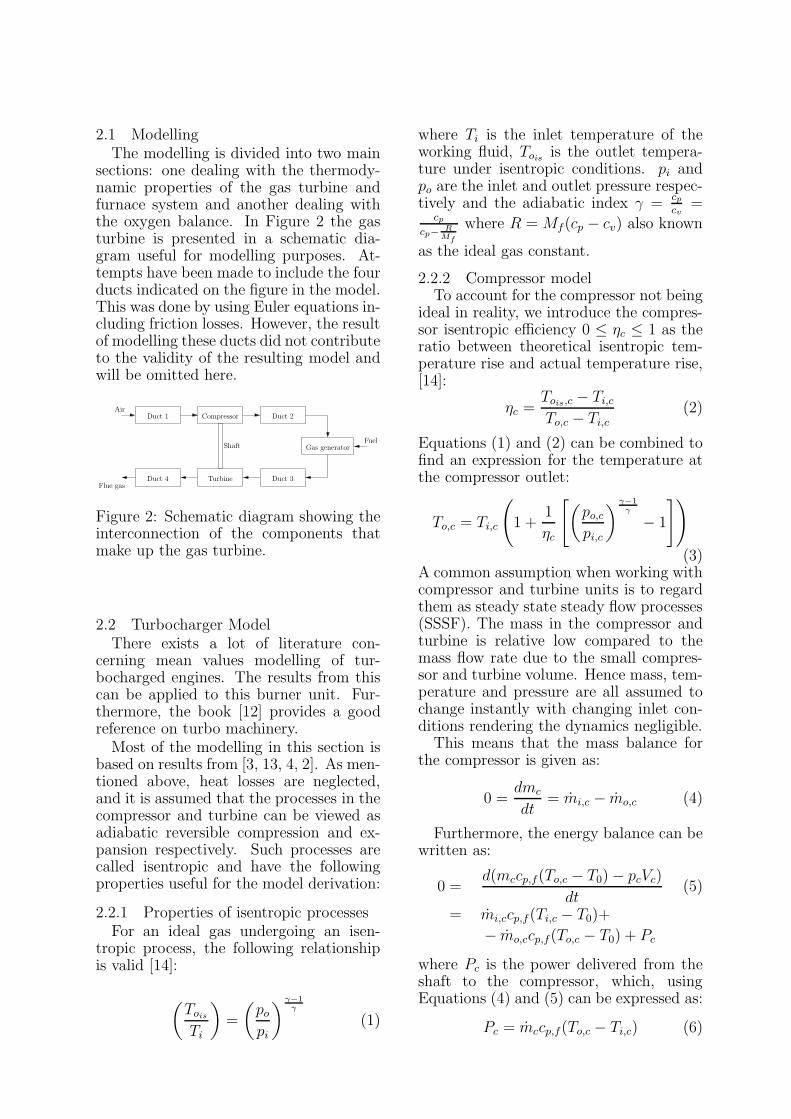
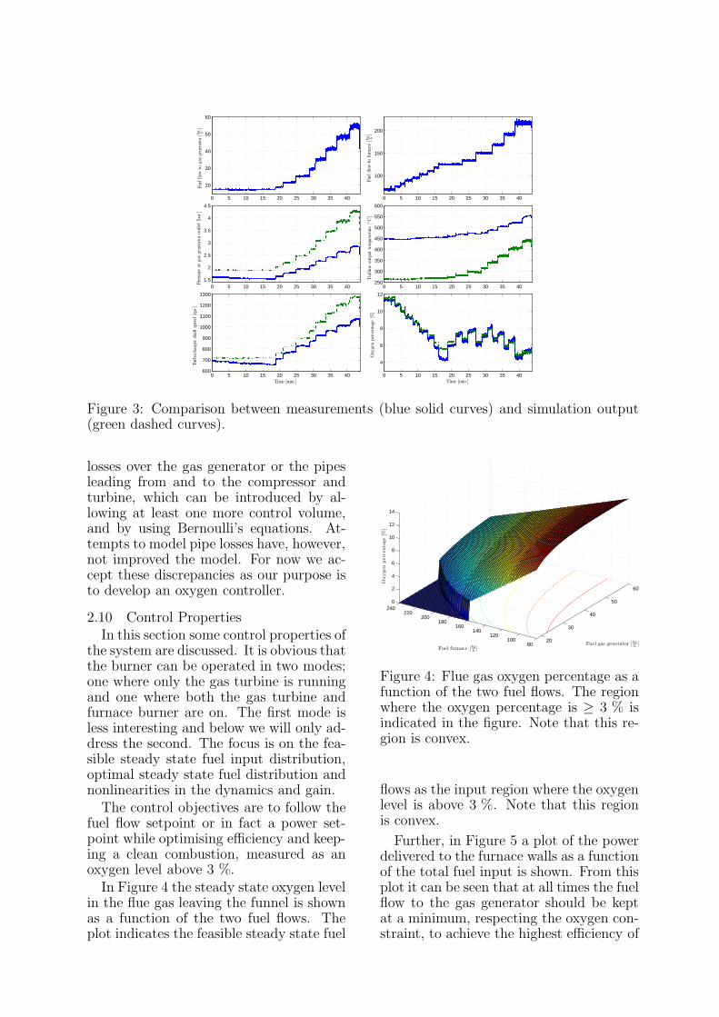
In Figure 4 the steady state oxygen levelin the flue gas leaving the funnel is shownas a function of the two fuel flows. Theplot indicates the feasible steady state fuel

20

30

40

50

60

80100

120140

160180

200220

2400

2

4

6

8

10

12

14

Fuel gas generator [kg

h]

Fuel furnace [kg

h]

Oxyge

nper

centa

ge[%

]

Figure 4: Flue gas oxygen percentage as afunction of the two fuel flows. The regionwhere the oxygen percentage is ≥ 3 % isindicated in the figure. Note that this re-gion is convex.

flows as the input region where the oxygenlevel is above 3 %. Note that this regionis convex.

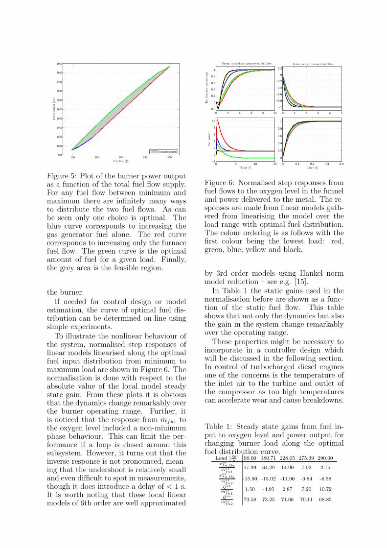
Further, in Figure 5 a plot of the powerdelivered to the furnace walls as a functionof the total fuel input is shown. From thisplot it can be seen that at all times the fuelflow to the gas generator should be keptat a minimum, respecting the oxygen con-straint, to achieve the highest efficiency of

100 150 200 250 300800

1000

1200

1400

1600

1800

2000

2200

2400

2600

2800

Fuel flow [kg

h]

Pow

erou

tput

[kW

]

Feasible region

Figure 5: Plot of the burner power outputas a function of the total fuel flow supply.For any fuel flow between minimum andmaximum there are infinitely many waysto distribute the two fuel flows. As canbe seen only one choice is optimal. Theblue curve corresponds to increasing thegas generator fuel alone. The red curvecorresponds to increasing only the furnacefuel flow. The green curve is the optimalamount of fuel for a given load. Finally,the grey area is the feasible region.

the burner.If needed for control design or model

estimation, the curve of optimal fuel dis-tribution can be determined on line usingsimple experiments.

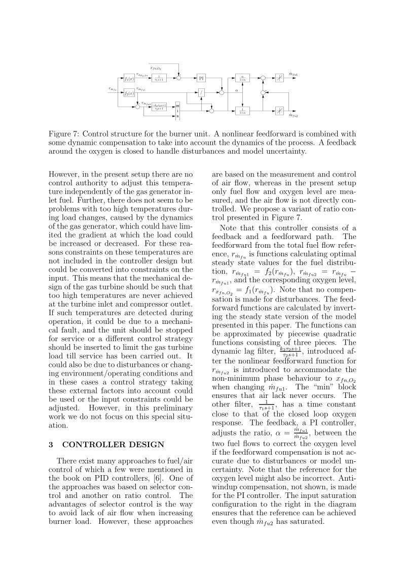
To illustrate the nonlinear behaviour ofthe system, normalised step responses oflinear models linearised along the optimalfuel input distribution from minimum tomaximum load are shown in Figure 6. Thenormalisation is done with respect to theabsolute value of the local model steadystate gain. From these plots it is obviousthat the dynamics change remarkably overthe burner operating range. Further, itis noticed that the response from mfu1 tothe oxygen level included a non-minimumphase behaviour. This can limit the per-formance if a loop is closed around thissubsystem. However, it turns out that theinverse response is not pronounced, mean-ing that the undershoot is relatively smalland even difficult to spot in measurements,though it does introduce a delay of < 1 s.It is worth noting that these local linearmodels of 6th order are well approximated

0 5 10 15−2

0

2

4

6

8

10

Time [s]

To:

pow

er

0 2 4 6 8 10−0.2

0

0.2

0.4

0.6

0.8

1

From: scaled gas generator fuel flow

To:

Oxygen

per

centa

ge

0 0.1 0.2 0.3 0.4

0

0.2

0.4

0.6

0.8

1

Time [s]

0 1 2 3 4 5

−1

−0.8

−0.6

−0.4

−0.2

0

0.2

From: scaled furnace fuel flow

Figure 6: Normalised step responses fromfuel flows to the oxygen level in the funneland power delivered to the metal. The re-sponses are made from linear models gath-ered from linearising the model over theload range with optimal fuel distribution.The colour ordering is as follows with thefirst colour being the lowest load: red,green, blue, yellow and black.

by 3rd order models using Hankel normmodel reduction – see e.g. [15].

In Table 1 the static gains used in thenormalisation before are shown as a func-tion of the static fuel flow. This tableshows that not only the dynamics but alsothe gain in the system change remarkablyover the operating range.

These properties might be necessary toincorporate in a controller design whichwill be discussed in the following section.In control of turbocharged diesel enginesone of the concerns is the temperature ofthe inlet air to the turbine and outlet ofthe compressor as too high temperaturescan accelerate wear and cause breakdowns.

Table 1: Steady state gains from fuel in-put to oxygen level and power output forchanging burner load along the optimalfuel distribution curve.

Load [ kg

h] 98.00 180.71 228.05 275.39 290.00

xssfn,O2

mssfu1

17.99 34.29 14.90 7.02 2.75

xssfn,O2

mssfu2

-15.90 -15.02 -11.90 -9.84 -8.58

Qss

mssfu1

1.50 -4.95 2.87 7.20 10.72

Qss

mssfu2

73.58 73.25 71.66 70.11 68.85

min

/

α1+α

11+α

PI1

τ1s+1

f2(x)

−k2τ2s+1τ2s+1

-

mfu2

mfu1

rmfu α

-

- rmfu2

rmfu1

f1(x)

xfn,O2

rxO2,fn

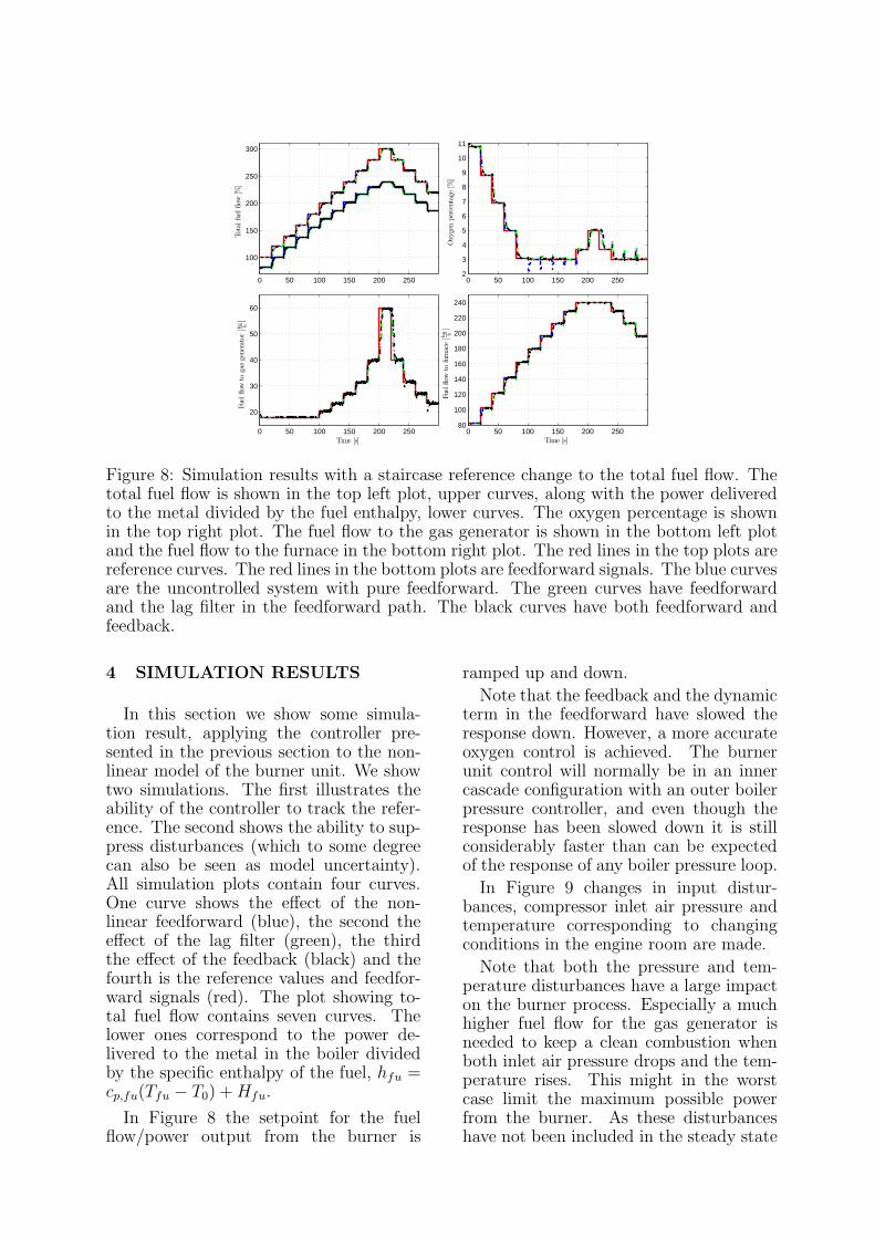
Figure 7: Control structure for the burner unit. A nonlinear feedforward is combined withsome dynamic compensation to take into account the dynamics of the process. A feedbackaround the oxygen is closed to handle disturbances and model uncertainty.

However, in the present setup there are nocontrol authority to adjust this tempera-ture independently of the gas generator in-let fuel. Further, there does not seem to beproblems with too high temperatures dur-ing load changes, caused by the dynamicsof the gas generator, which could have lim-ited the gradient at which the load couldbe increased or decreased. For these rea-sons constraints on these temperatures arenot included in the controller design butcould be converted into constraints on theinput. This means that the mechanical de-sign of the gas turbine should be such thattoo high temperatures are never achievedat the turbine inlet and compressor outlet.If such temperatures are detected duringoperation, it could be due to a mechani-cal fault, and the unit should be stoppedfor service or a different control strategyshould be inserted to limit the gas turbineload till service has been carried out. Itcould also be due to disturbances or chang-ing environment/operating conditions andin these cases a control strategy takingthese external factors into account couldbe used or the input constraints could beadjusted. However, in this preliminarywork we do not focus on this special situ-ation.

3 CONTROLLER DESIGN

There exist many approaches to fuel/aircontrol of which a few were mentioned inthe book on PID controllers, [6]. One ofthe approaches was based on selector con-trol and another on ratio control. Theadvantages of selector control is the wayto avoid lack of air flow when increasingburner load. However, these approaches

are based on the measurement and controlof air flow, whereas in the present setuponly fuel flow and oxygen level are mea-sured, and the air flow is not directly con-trolled. We propose a variant of ratio con-trol presented in Figure 7.

Note that this controller consists of afeedback and a feedforward path. Thefeedforward from the total fuel flow refer-ence, rmfu

is functions calculating optimalsteady state values for the fuel distribu-tion, rmfu1

= f2(rmfu), rmfu2

= rmfu−

rmfu1, and the corresponding oxygen level,

rxfn,O2= f1(rmfu

). Note that no compen-sation is made for disturbances. The feed-forward functions are calculated by invert-ing the steady state version of the modelpresented in this paper. The functions canbe approximated by piecewise quadraticfunctions consisting of three pieces. Thedynamic lag filter, k2τ2s+1

τ2s+1, introduced af-

ter the nonlinear feedforward function forrmfu2

is introduced to accommodate thenon-minimum phase behaviour to xfn,O2

when changing mfu1. The “min” blockensures that air lack never occurs. Theother filter, 1

τ1s+1, has a time constant

close to that of the closed loop oxygenresponse. The feedback, a PI controller,

adjusts the ratio, α =mfu1

mfu2, between the

two fuel flows to correct the oxygen levelif the feedforward compensation is not ac-curate due to disturbances or model un-certainty. Note that the reference for theoxygen level might also be incorrect. Anti-windup compensation, not shown, is madefor the PI controller. The input saturationconfiguration to the right in the diagramensures that the reference can be achievedeven though mfu2 has saturated.

0 50 100 150 200 250

100

150

200

250

300

Tot

alfu

elflo

w[%

]

0 50 100 150 200 2502

3

4

5

6

7

8

9

10

11

Oxy

gen

per

cent

age

[%]

0 50 100 150 200 250

20

30

40

50

60

Time [s]

Fuel

flow

toga

sge

nera

tor[k

g h]

0 50 100 150 200 25080

100

120

140

160

180

200

220

240

Time [s]Fu

elflo

wto

furn

ace

[kg h]

Figure 8: Simulation results with a staircase reference change to the total fuel flow. Thetotal fuel flow is shown in the top left plot, upper curves, along with the power deliveredto the metal divided by the fuel enthalpy, lower curves. The oxygen percentage is shownin the top right plot. The fuel flow to the gas generator is shown in the bottom left plotand the fuel flow to the furnace in the bottom right plot. The red lines in the top plots arereference curves. The red lines in the bottom plots are feedforward signals. The blue curvesare the uncontrolled system with pure feedforward. The green curves have feedforwardand the lag filter in the feedforward path. The black curves have both feedforward andfeedback.

4 SIMULATION RESULTS

In this section we show some simula-tion result, applying the controller pre-sented in the previous section to the non-linear model of the burner unit. We showtwo simulations. The first illustrates theability of the controller to track the refer-ence. The second shows the ability to sup-press disturbances (which to some degreecan also be seen as model uncertainty).All simulation plots contain four curves.One curve shows the effect of the non-linear feedforward (blue), the second theeffect of the lag filter (green), the thirdthe effect of the feedback (black) and thefourth is the reference values and feedfor-ward signals (red). The plot showing to-tal fuel flow contains seven curves. Thelower ones correspond to the power de-livered to the metal in the boiler dividedby the specific enthalpy of the fuel, hfu =cp,fu(Tfu − T0) + Hfu.

In Figure 8 the setpoint for the fuelflow/power output from the burner is

ramped up and down.

Note that the feedback and the dynamicterm in the feedforward have slowed theresponse down. However, a more accurateoxygen control is achieved. The burnerunit control will normally be in an innercascade configuration with an outer boilerpressure controller, and even though theresponse has been slowed down it is stillconsiderably faster than can be expectedof the response of any boiler pressure loop.

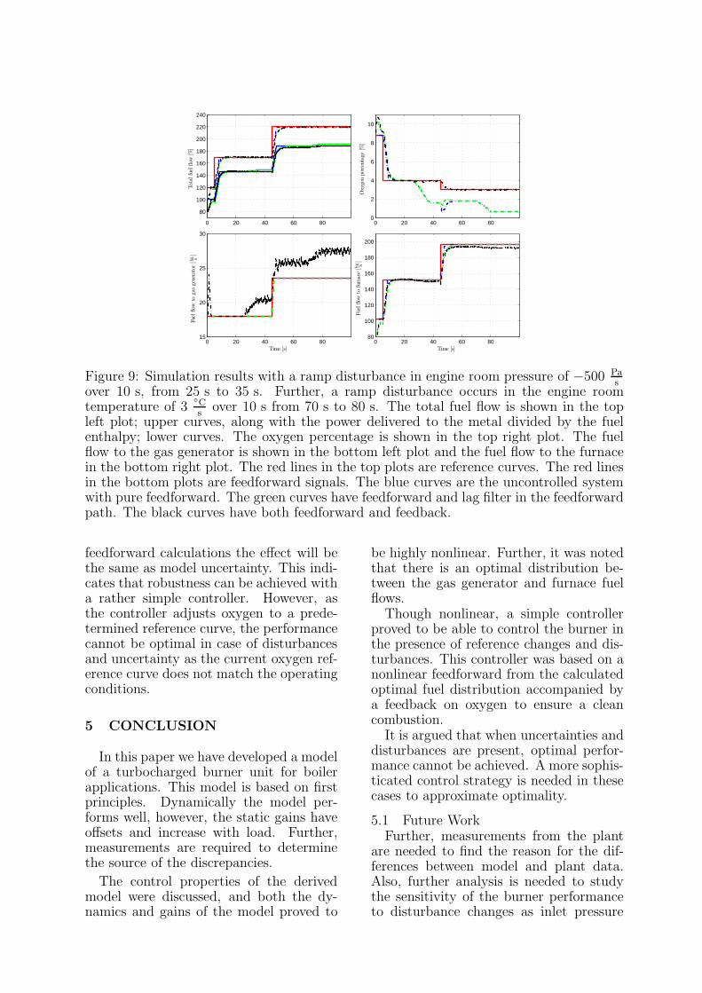
In Figure 9 changes in input distur-bances, compressor inlet air pressure andtemperature corresponding to changingconditions in the engine room are made.

Note that both the pressure and tem-perature disturbances have a large impacton the burner process. Especially a muchhigher fuel flow for the gas generator isneeded to keep a clean combustion whenboth inlet air pressure drops and the tem-perature rises. This might in the worstcase limit the maximum possible powerfrom the burner. As these disturbanceshave not been included in the steady state

0 20 40 60 80

80

100

120

140

160

180

200

220

240

Tot

alfu

elflo

w[%

]

0 20 40 60 800

2

4

6

8

10

Oxy

gen

per

cent

age

[%]

0 20 40 60 8015

20

25

30

Time [s]

Fuel

flow

toga

sge

nera

tor[k

g h]

0 20 40 60 8080

100

120

140

160

180

200

Time [s]

Fuel

flow

tofu

rnac

e[k

g h]

Figure 9: Simulation results with a ramp disturbance in engine room pressure of −500 Pas

over 10 s, from 25 s to 35 s. Further, a ramp disturbance occurs in the engine roomtemperature of 3

◦Cs

over 10 s from 70 s to 80 s. The total fuel flow is shown in the topleft plot; upper curves, along with the power delivered to the metal divided by the fuelenthalpy; lower curves. The oxygen percentage is shown in the top right plot. The fuelflow to the gas generator is shown in the bottom left plot and the fuel flow to the furnacein the bottom right plot. The red lines in the top plots are reference curves. The red linesin the bottom plots are feedforward signals. The blue curves are the uncontrolled systemwith pure feedforward. The green curves have feedforward and lag filter in the feedforwardpath. The black curves have both feedforward and feedback.

feedforward calculations the effect will bethe same as model uncertainty. This indi-cates that robustness can be achieved witha rather simple controller. However, asthe controller adjusts oxygen to a prede-termined reference curve, the performancecannot be optimal in case of disturbancesand uncertainty as the current oxygen ref-erence curve does not match the operatingconditions.

5 CONCLUSION

In this paper we have developed a modelof a turbocharged burner unit for boilerapplications. This model is based on firstprinciples. Dynamically the model per-forms well, however, the static gains haveoffsets and increase with load. Further,measurements are required to determinethe source of the discrepancies.

The control properties of the derivedmodel were discussed, and both the dy-namics and gains of the model proved to

be highly nonlinear. Further, it was notedthat there is an optimal distribution be-tween the gas generator and furnace fuelflows.

Though nonlinear, a simple controllerproved to be able to control the burner inthe presence of reference changes and dis-turbances. This controller was based on anonlinear feedforward from the calculatedoptimal fuel distribution accompanied bya feedback on oxygen to ensure a cleancombustion.

It is argued that when uncertainties anddisturbances are present, optimal perfor-mance cannot be achieved. A more sophis-ticated control strategy is needed in thesecases to approximate optimality.

5.1 Future WorkFurther, measurements from the plant

are needed to find the reason for the dif-ferences between model and plant data.Also, further analysis is needed to studythe sensitivity of the burner performanceto disturbance changes as inlet pressure

and temperature. Also, does the plantdynamics and gains change remarkably asthe disturbance changes?

A simple nonlinear model for the gasgenerator can be derived by neglectingvariations in mass and internal energy –see [5].

A control strategy that is particularlysuited for this type of control problem isMPC. The reason for this is that MPCnaturally handles the constraints presenton input and process variables. Further,a model of the disturbances can easily beintroduced and optimal performance canbe approximated. However, application oflinear MPC shows poor performance pos-sibly due to the nonlinearities in the plant.This means that one could consider non-linear MPC or linear MPC with multiplemodels or perhaps simple multiple nonlin-ear models. It should here be noted thatthe feasible input region was found to beconvex.

REFERENCES

[1] J. P. Jensen, A. F. Kristensen, S. C.Sorenson, N. Houbak, E. Hendricks,Mean value modelling of a small tur-bocharged diesel engine, SAE Techni-cal Paper Series No. 910070.

[2] M. Muller, E. Hendricks, S. C.Sorenson, Mean valve modelling ofturbocharged spark ignition engines,SAE Technical Paper Series 980784(1998) 125–145.

[3] I. Kolmanovsky, P. Moraal, Tur-bocharger modeling for automotivecontrol applications, SAE TechnicalPaper Series 1999-01-0908.

[4] M. Jung, K. Glover, Control-orientedlinear parameter-varying modelling ofa turbocharged diesel engine, in: Pro-ceedings of the IEEE Conference onControl Applications, 2003.

[5] R. Sekhon, H. Bassily, J. Wagner,J. Gaddis, Stationary gas turbines – areal time dynamic model with experi-mental validation, in: American Con-

trol Conference, Minneapolis, Min-nesota, USA, 2006.

[6] K. J. Astrom, T. Hagglund, Ad-vanced PID Control, ISA - Instru-mentation, Systems, and AutomationSociety, 2006.

[7] J. M. Maciejowski, Predictive ControlWith Constraints, Harlow: PearsonEducation Limited, 2001.

[8] J. A. Rossiter, Model-based Predic-tive Control: A Practical Approach,CRC Press LLC, 2003.

[9] S. J. Qin, T. A. Badgwell, A surveyof industrial model predictive con-trol technology, Control EngineeringPractice 11 (2003) 733–764.

[10] R. B. Persson, B. V. Sørensen, Hybridcontrol of a compact marine boilersystem, Master’s thesis, Aalborg Uni-versity, Institute of Electronic Sys-tems (2006).

[11] P. U. Hvistendahl, B. Solberg, Mod-elling and multi variable control of amarine boiler, Master’s thesis, Aal-borg Universitet, Institute of Elec-tronic Systems, Aalborg, Denmark(2004).

[12] H. I. H. Saravanamuttoo, G. F. C.Rogers, H. Cohen, Gas Turbine The-ory, 5th Edition, Prentice Hall, 2001.

[13] A. Amstutz, L. Guzzella, Control ofdiesel engines, IEEE Control SystemsMagazine 18 (5) (1998) 53–71.

[14] T. D. Eastop, A. McConkey, Ap-plied Thermodynamics for Engineer-ing Technologists, Addison WesleyLongman, 1993.

[15] K. Zhou, J. Doyle, K. Glover, Ro-bust and Optimal Control, New Jer-sey: Prentice-Hall, Inc, 1996.