MODELING UNCERTAINTIES AND NEAR-ROAD PM2.5: A COMPARISON OF CALINE4, CAL3QHC AND AERMOD

Task Order Numbers 67 and 80

August 21, 2008

By

Hao Chen, MS Song Bai, PhD

Douglas Eisinger, PhD Deb Niemeier, PhD, PE Michael Claggett, PhD*

Abstract

Background: Scientific evidence has shown an association between particulate matter exposure and adverse human health impacts. Accurately predicting near-road PM2.5 concentrations is therefore important for project-level transportation conformity and health risk analyses. Methods: This study assessed the capability and performance of three dispersion models, CALINE4, CAL3QHC, and AERMOD, in predicting near-road PM2.5 concentrations. The comparative assessment included identifying differences among the three models in terms of methodology and data requirements. An intersection in Sacramento, California and a busy road in London, United Kingdom were used as sampling sites to evaluate how model predictions differed from observed PM2.5 concentrations. Results: Screen plots and statistical tests indicated that, at the Sacramento site, CALINE4 and CAL3QHC performed moderately well, while AERMOD under-predicted PM2.5 concentrations. For the London site, both CALINE4 and CAL3QHC resulted in over-predictions when incremental concentrations due to on-road emission sources were low, while under-predictions occurred when incremental concentrations were high. The street canyon effect and receptor location likely contributed to the relatively poor performance of the models at the London site.

* With the U.S. Federal Highway Administration; other authors are with the U.C. Davis-Caltrans Air Quality Project.

About The U.C. Davis-Caltrans Air Quality Project

http://AQP.engr.ucdavis.edu/

Department of Civil & Environmental Engineering University of California

One Shields Ave., Davis, CA 95616 (530) 752-0586

Mission: The Air Quality Project (AQP) seeks to advance understanding of transportation related air quality problems, develop advanced modeling and analysis capability within the transportation and air quality planning community, and foster collaboration among agencies to improve mobility and achieve air quality goals. History: Since the 1990s, the U.S. Federal Highway Administration and Caltrans have funded the AQP to provide transportation-related air quality support. Caltrans and AQP researchers identify and resolve issues that could slow clean air progress and transportation improvements. Accessibility: AQP written materials and software tools are distributed through our website, peer-reviewed publications, conference presentations, training classes, formal reports and technical memoranda, and periodic newsletters. Research: AQP investigations focus on project-level, regional-scale, and national-level assessments. Tools and publication topics cover pollutant-specific problems such as those involving particulate matter, carbon monoxide, carbon dioxide, ozone and air toxics; activity data collection and assessment for on- and off-road vehicles and equipment; mitigation options such as transportation control measures; policy analyses addressing transportation conformity and state implementation plan development; litigation support; and goods movement assessments.

Project Management

Principal Investigator and Director: Deb Niemeier, PhD, PE Program Manager: Douglas Eisinger, PhD

Caltrans Project Manager: Mike Brady, Senior Environmental Planner

Air Quality and Conformity Coordination Division of Transportation Planning, MS-32

California Department of Transportation 1120 N Street, Sacramento, CA 94274

(916) 653-0158

iii

Acknowledgements

This research was partly funded through the UC Davis‐Caltrans Air Quality Project. The authors

thank Elizabeth Yura at the California Air Resources Board, Neil Wheeler and Stephanie Bratek

at Sonoma Technology, Inc. and William Crowl at the traffic Operations Center of the County of

Sacramento for their assistance in data collection and model specification.

iv

Table of Contents

Acknowledgements.........................................................................................................................iii

List of Tables ...................................................................................................................................vi

List of Figures .................................................................................................................................vii

1 Introduction ............................................................................................................................ 1

1.1 Problem Statement......................................................................................................... 1

1.2 Study Objectives ............................................................................................................. 2

1.3 Organization of the Report ............................................................................................. 2

2 Literature Review.................................................................................................................... 3

2.1 Negative Impact of PM2.5 and the Role of Vehicle PM2.5 Emissions............................... 3

2.2 Dispersion Models – Brief Literature Review ................................................................. 4

2.2.1 CALINE4................................................................................................................... 5

2.2.2 CAL3QHC ................................................................................................................. 6

2.2.3 AERMOD.................................................................................................................. 7

2.2.4 PM Prediction by Other Models ............................................................................. 8

3 Model Description .................................................................................................................. 9

3.1 CALINE4........................................................................................................................... 9

3.2 CAL3QHC ....................................................................................................................... 10

3.3 AERMOD........................................................................................................................ 10

3.4 Data Requirements ....................................................................................................... 13

4 Case Study – Background and Model Setup ......................................................................... 15

v

4.1 Study Area..................................................................................................................... 15

4.2 Observed PM2.5 Concentrations ................................................................................... 18

4.3 Model Inputs................................................................................................................. 20

4.3.1 Emission Factor (EF).............................................................................................. 20

4.3.2 Deposition and Settling Velocities ........................................................................ 22

5 Case Study – Results and Analysis ........................................................................................ 23

5.1 Screen Plots and Descriptive Statistics ......................................................................... 23

5.1.1 Factor‐of‐Two Plots............................................................................................... 23

5.1.2 Difference Overview and Patterns........................................................................ 25

5.1.3 Correlation between Estimated and Observed Concentrations .......................... 28

5.2 Statistical Tests ............................................................................................................. 29

5.2.1 Test of Prediction Bias .......................................................................................... 30

5.2.2 Test of Prediction Trend ....................................................................................... 31

5.2.3 Test for Model Difference..................................................................................... 32

5.3 Distribution Patterns..................................................................................................... 34

6 Discussion and Conclusion.................................................................................................... 36

References .................................................................................................................................... 40

Appendix A: Documentation of Steps to Complete Model Runs ................................................ 44

A.1 CALINE4......................................................................................................................... 44

A.2 CAL3QHC ....................................................................................................................... 49

A.3 AERMOD........................................................................................................................ 54

Appendix B: Abbreviations........................................................................................................... 64

vi

List of Tables

Table 3‐1 Data Requirements of CALINE4, CAL3QHC, and AERMOD ........................................... 14

Table 4‐1 PM2.5 Concentrations (µg/m3) at the Sacramento Site................................................ 18

Table 4‐2 Emission factors of PM2.5 (g/VKT) .............................................................................. 21

Table 5‐1 Percentage of Points Falling in the Factor‐of‐two Envelope ....................................... 25

Table 5‐2 Difference Overview (values are in µg/m3).................................................................. 26

Table 5‐3 R2 correlating model‐predicted and observed concentrations.................................... 29

Table 5‐4 Test Results for Prediction Bias.................................................................................... 31

Table 5‐5 Test Result for Prediction Trend. ................................................................................. 32

Table A‐ 1 CALINE4 Input Description 45

Table A‐ 2 CAL3QHC Input Description 49

Table A‐ 3 Explanation of Surface Observation Input for Stage 2 55

Table A‐ 4 Explanation of Upper Air Sounding Input for Stage 2 57

Table A‐ 5 Explanation of Part of AERMET3.INP 59

Table A‐ 6 Explanation of Part of AERMOD.INP 62

vii

List of Figures

Figure 4‐1 Sacramento Site Layout ........................................................................................... 15

Figure 4‐2 London Site Layout ..................................................................................................... 17

Figure 4‐3 Background Proportion Plots (Sacramento Case) ...................................................... 19

Figure 5‐1 Factor‐of‐Two Plots (all concentrations are in µg/m3). .............................................. 24

Figure 5‐2 (part 2) Pattern of (all concentrations are in µg/m3). ........................................... 28

Figure 5‐3 Cumulative Frequency Distributions of Observed Concentrations (solid lines) and

Predicted Concentrations (dotted lines) (all concentrations are in µg/m3). ................................ 35

Figure A‐ 1 AERMET Process 54

1

1 Introduction

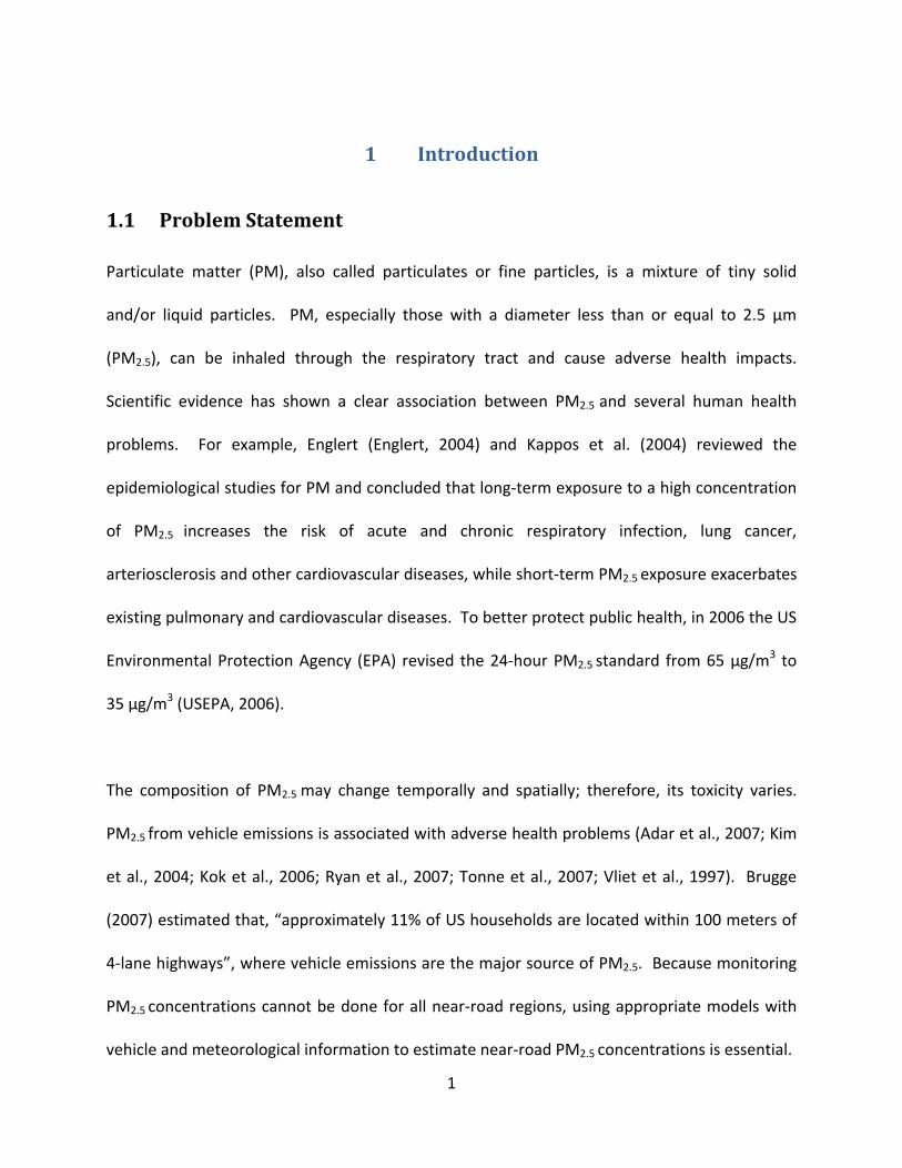
1.1 Problem Statement

Particulate matter (PM), also called particulates or fine particles, is a mixture of tiny solid

and/or liquid particles. PM, especially those with a diameter less than or equal to 2.5 µm

(PM2.5), can be inhaled through the respiratory tract and cause adverse health impacts.

Scientific evidence has shown a clear association between PM2.5 and several human health

problems. For example, Englert (Englert, 2004) and Kappos et al. (2004) reviewed the

epidemiological studies for PM and concluded that long‐term exposure to a high concentration

of PM2.5 increases the risk of acute and chronic respiratory infection, lung cancer,

arteriosclerosis and other cardiovascular diseases, while short‐term PM2.5 exposure exacerbates

existing pulmonary and cardiovascular diseases. To better protect public health, in 2006 the US

Environmental Protection Agency (EPA) revised the 24‐hour PM2.5 standard from 65 µg/m3 to

35 µg/m3 (USEPA, 2006).

The composition of PM2.5 may change temporally and spatially; therefore, its toxicity varies.

PM2.5 from vehicle emissions is associated with adverse health problems (Adar et al., 2007; Kim

et al., 2004; Kok et al., 2006; Ryan et al., 2007; Tonne et al., 2007; Vliet et al., 1997). Brugge

(2007) estimated that, “approximately 11% of US households are located within 100 meters of

4‐lane highways”, where vehicle emissions are the major source of PM2.5. Because monitoring

PM2.5 concentrations cannot be done for all near‐road regions, using appropriate models with

vehicle and meteorological information to estimate near‐road PM2.5 concentrations is essential.

2

1.2 Study Objectives

Air dispersion models used to estimate gas concentrations are used for predicting near‐road

particle concentrations. In this study, the capabilities and features of three dispersion models,

CALINE4, CAL3QHC and AERMOD, are evaluated. Specifically, the research objectives are to

examine the performance of the three models individually based on their predictions of PM2.5

concentrations at two sites, an intersection of Florin Road and Stockton Boulevard in

Sacramento, California and a busy road in London, United Kingdom. Hypotheses, such as

whether the model over or under‐predicts the concentrations, whether the model under‐

prediction increases with observed concentration, and whether the three models are

significantly different, are tested. The research aims to identify the models that are appropriate

for predicting near‐road PM2.5 concentrations.

1.3 Organization of the Report

This report consists of six chapters and one appendix. Chapters 1 and 2 introduce the research

background, clarify the study objectives and review previous related studies. Chapter 3

introduces and compares the three models from the theoretical perspective. Chapters 4 and 5

evaluate the three models through their performances at two sites. Chapter 6 summarizes the

major results of this study and discusses future research. The appendix provides step‐by‐step

instructions to run the three models.

3

2 Literature Review

2.1 Negative Impact of PM2.5 and the Role of Vehicle PM2.5 Emissions

Studies show a relationship between PM exposure and adverse human health impacts,

regarding fine particles (PM2.5), as well as coarse particles (PM2.5‐10). The US EPA, in the report

“Particulate Matter Research Program: Five Years of Progress” (2004b), reviewed critical studies

of PM and found that ambient PM2.5 exposure is associated with morbidity and mortality

caused by respiratory and cardiovascular diseases.

Because PM2.5 is a complex mixture of organic and inorganic components, its composition

varies temporally and spatially. Jerrett and Finkelstein (2005) showed that the toxicity of PM2.5

varies for different States throughout the United States. Davidson et al. (2005) showed that

health problems are associated with particle size and composition. Schlesinger (2007)

examined the toxicity of common inorganic components of PM2.5 and found clear adverse

biological effects from some secondary acidic sulfates. He also indicated that different

components were responsible for different adverse health outcomes.

Research has also shown that PM2.5 that originated from vehicle emissions falls in the toxic

category (Kok et al., 2006). Adar et al. (2007) conducted a study in suburban St. Louis, Missouri

for elders and found a negative association between PM2.5 and heart rate variability; the short‐

term association was mainly limited to traffic‐related PM2.5 rather than PM2.5 from other

4

sources. Other studies showed a relationship between near‐highway PM2.5 and childhood

asthma, lung cancer, myocardial infarction and other health problems (Kim et al., 2004; Ryan et

al., 2007; Tonne et al., 2007; Vineis, 2006). Therefore, knowing the PM2.5 concentrations in

regions near motorways is essential.

2.2 Dispersion Models – Brief Literature Review

There are various gas dispersion models. Holmes and Morawska (2006) reviewed previous

studies which measured both gas and PM concentrations at the same time and concluded that

gas and PM concentrations correlated quite well in an open environment.

The most widely used air dispersion models are the Gaussian models, which are based on two

modified Gaussian distributions of the plume in the vertical and horizontal directions. Three

Gaussian models, CALINE4, CAL3QHC and AERMOD, are used to predict near‐road PM2.5

concentrations in this study. CALINE4 has been widely used in California to evaluate

transportation project‐level air quality impacts; CAL3QHC is designed for carbon monoxide (CO)

and PM concentrations and is one model suggested by EPA for dispersion modeling; AERMOD is

an additional EPA‐recommended model for dispersion modeling. All three models have been

widely used to model gaseous pollutants. They have also been used to model PM

concentrations in some limited applications.

5

2.2.1 CALINE4

The CALINE4 model is widely used to predict near‐road vehicle emissions. This model has been

tested and validated for predicting concentrations of several vehicle‐emitted pollutants near‐

road under certain conditions, such as CO, oxides of nitrogen (NOx), and additional gases.

Loranger et al. (1995) showed that CALINE4 predicted near‐road CO concentrations well, but

under‐predicted manganese (Mn) concentrations. Broderick et al. (2005) examined CALINE4’s

performance of modeling transportation‐related CO for a free‐flowing motorway and a

periodically congested roundabout in Ireland and concluded that CALINE4 functioned well

under stable atmospheric conditions but performed poorly under low wind conditions.

Marmur and Mamane (2003) showed that CALINE4, together with emission factors predicted

by COPERT III, is suitable for near‐road NOx concentration prediction in open urban and rural

sites in Israel, though this conclusion may not be extended to dense urban center locations.

Levitin et al. (2005) showed that CALINE4 performed well for near‐road NOx and nitrogen

dioxide (NO2) concentrations prediction. Kenty et al. (2007) showed CALINE4 predicts NOx

concentration well, but under‐predicts NO2 concentrations probably due to assumptions

imbedded in the model.

Jones et al. (1998) showed that CALINE4 predicts well for daytime 12‐hour average

concentrations of transportation related benzene, toluene, ethylbenzene and xylene in urban

areas. Broderick and O’Donoghue (2007) examined CALINE4’s capability in predicting

6

transportation related emissions of seven inert gases – n‐Pentane, Iso‐pentane, Ethene,

Propene, 1,3‐Butadiene, Acetylene and Benzene under low wind speeds and showed that

CALINE4, together with emission factors predicted by COPERT III, gives good long‐term

estimations but underestimates higher percentile concentrations when evaluating short‐term

conditions.

CALINE4 has also been tested in predicting particle concentrations in two studies. Gramotnev

et al. (2003) used a modified version of CALINE4 to estimate motor vehicle emission factors of

fine and ultrafine particles near a busy road in the Brisbane area in Australia. Employing the

resulting emission factors, they found that the CALINE4 model results matched the observed

rate of dispersion with distance from the road well. Findings in the second study were mixed:

CALINE4 performed well for an intersection in Sacramento site but not for urban road in

London site (Yura et al., 2007) [note that this study reevaluates the same sites examined by

Yura et al.].

2.2.2 CAL3QHC

CAL3QHC is designed for CO and PM concentration prediction. Studies to date on model

performance have been mixed. Moseholm et al. (1996) showed that CAL3QHC yielded

unsatisfying results under conditions involving low wind speeds and nearby tall buildings. Not

unsurprisingly, Zhou and Sperling (2001) note that mixed traffic (bicycles and vehicles) and

near‐road high‐rise buildings will cause CAL3QHC to poorly predict CO concentrations. An

extensive evaluation of the CAL3QHC model was provided in a National Cooperative Highway

7

Research Program study (Carr et al., 2002) as part of the development of the Hybrid Roadway

Intersection model (HYROAD). This report documents poor model performance at ten sites

across the country, 3 where intensive CO monitoring was conducted plus an additional 7 with

less intensive monitoring. However, CAL3QHC was shown to perform well generally in open

areas with moderate traffic volumes (Abdul‐Wahab, 2004) and along moderately trafficked

suburban roads (Kho et al., 2007). CAL3QHC has also been used with somewhat less success to

estimate both transportation‐related PM2.5 and PM10 (Gokhale and Raokhade, 2008) – in which

the predicted concentrations did not match the measured concentrations well. PM dispersion

from non‐traffic sources may have been a main contributor to this mismatch.

2.2.3 AERMOD

AERMOD can be used for predicting the concentrations of various pollutants emitted by point,

line and area sources. This model is typically used for large areas (Faulkner et al., 2007; Hanna

et al., 2006; Jampana et al., 2004; Kumar et al., 2006; Stein et al., 2007; Touma et al., 2007) or

stationary sources (Orloff et al., 2006; Seigneur et al., 2006). Kesarkar et al. (2007) used

AERMOD to estimate PM10 concentrations over the city Puna in India and found that the model

generally underestimated PM10 concentrations except for residential areas. Zhang et al. (2008)

used AERMOD to estimate PM10 concentrations in the urban area of Hangzhou, China and

found that AERMOD underestimated concentrations; the authors noted that model

performance may have been related to lack of consideration of construction and secondary

particles. Although the model has not been widely used in predicting near‐road pollutant

8

concentrations, EPA recommends AERMOD to evaluate near‐road concentrations (USEPA,

Accessed July 10, 2008) and thus it is included in this study.

2.2.4 PM Prediction by Other Models

There are other models that have been used to predict PM2.5 or PM10 concentrations. Gokhale

and Raokhade (2008) used CALINE3 and the ‘Modified General Finite Line Source Model’ (M‐

GFLSM) to estimate transportation related PM2.5 and PM10 concentrations and found that both

of them performed worse than CAL3QHC generally. Vardoulakis et al. (2007) used three

dispersion models, WinOSPM (a Windows‐based version of OSPM), ADMS‐Urban 2.0 and

AEOLIUS Full, to estimate vehicle PM10 emissions from two streets in Birmingham and London

for one year and the models gave good estimates for PM10. The reason for the good match

partly relies on the high percentage of background concentration, which comprises

approximately 80% of the total PM10 concentration. Bowker et al. (2007) used the ‘Quick Urban

and Industrial Complex’ (QUIC) model to estimate the concentration of ultra fine particles near

I‐440 in Raleigh, North Carolina, and found that the predicted concentrations have a similar

pattern to the measured concentrations.

9

3 Model Description

CALINE4, CAL3QHC and AERMOD are all Gaussian models. They are based on two modified

Gaussian distributions of the plume in the vertical and horizontal directions. In addition, all

three models are steady‐state models; that is, the models assume that the dispersion process

takes no time to achieve the steady state. The material and equations presented in this chapter

are based on available model documentation.

3.1 CALINE4

CALINE4 is the most recent version of the CALINE model series developed by the California

Department of Transportation. It embeds the concept of mixing zone and uses modified

Gaussian distributions (Benson, 1984). CALINE4 uses a series of equivalent finite line sources to

represent the road segment, and models the whole region of finite line sources as a zone with

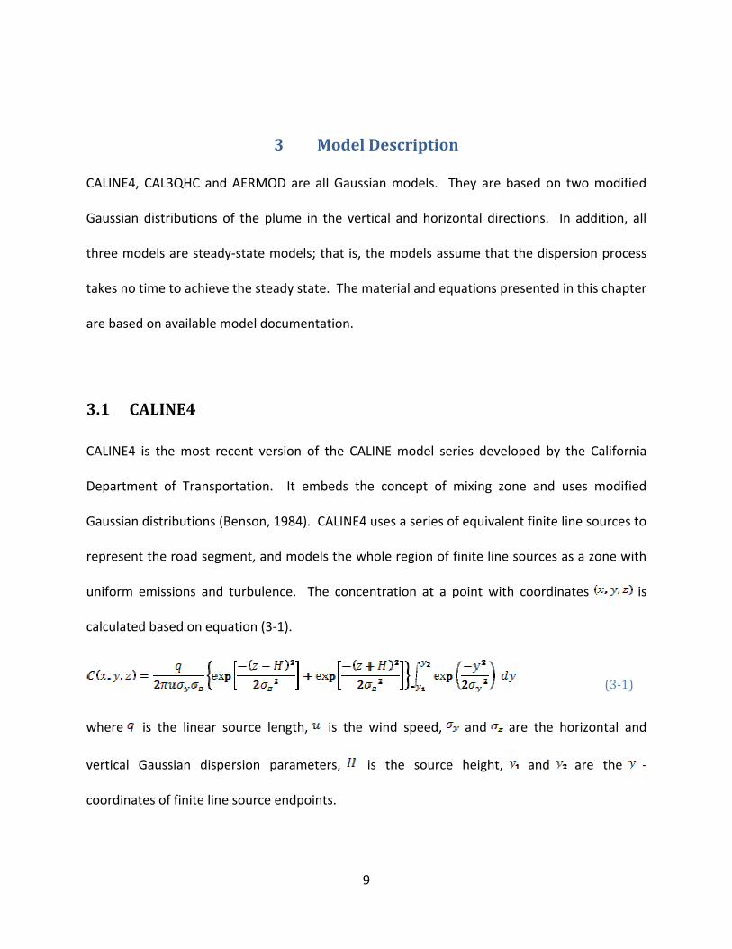
uniform emissions and turbulence. The concentration at a point with coordinates is

calculated based on equation (3‐1).

(3‐1)where is the linear source length, is the wind speed, and are the horizontal and

vertical Gaussian dispersion parameters, is the source height, and are the ‐

coordinates of finite line source endpoints.

10

Among all the variables, is a function of the ‐coordinate of the point where the

concentration is calculated and horizontal wind angle standard deviation; is modified by

incorporating the effects of vehicle‐induced heat.

3.2 CAL3QHC

CAL3QHC is an enhanced version of CALINE3 with an additional algorithm that estimates the

lengths of vehicular queues at signalized intersections (USEPA, 1995). Thus, CAL3QHC can

incorporate the emissions from idling vehicles as well as free‐flow traveling vehicles; although

the idling portion of the model was not evaluated as part of this study (refer to section 4.3).

The dispersion process formulated in CAL3QHC is the same as that in CALINE4 by applying

equation (3‐1). However, CAL3QHC uses atmospheric stability to estimate the horizontal

dispersion parameter ( ), and the vertical dispersion parameter ( ) is not modified by the

vehicle‐induced heat algorithm (Benson, 1992).

3.3 AERMOD

AERMOD incorporates the concept of planetary boundary layer (PBL) (USEPA, 2004a) – the

lowest part of the atmosphere and its characteristics that are directly affected by the earth’s

surface. There are two types of PBL: Stable Boundary Layer (SBL) and Convective Boundary

Layer (CBL). SBL occurs when the earth’s surface is colder than the air above, usually during the

night; and CBL otherwise. Whether the PBL is SBL or CBL, and the parameters of the boundary

layers, are determined by AERMET, a meteorological preprocessor used with AERMOD.

11

In SBL, two independent horizontal and vertical Gaussian distributions are used for modeling

pollutant dispersion, the same as is used in CALINE4 and CAL3QHC. In CBL, the horizontal

distribution is still Gaussian; however, the vertical distribution is a bi‐Gaussian distribution

(Cimorelli et al., 2005) and the concentration is calculated as a weighted average of two

Gaussian distributions; this is the main difference between AERMOD and CALINE4/CAL3QHC.

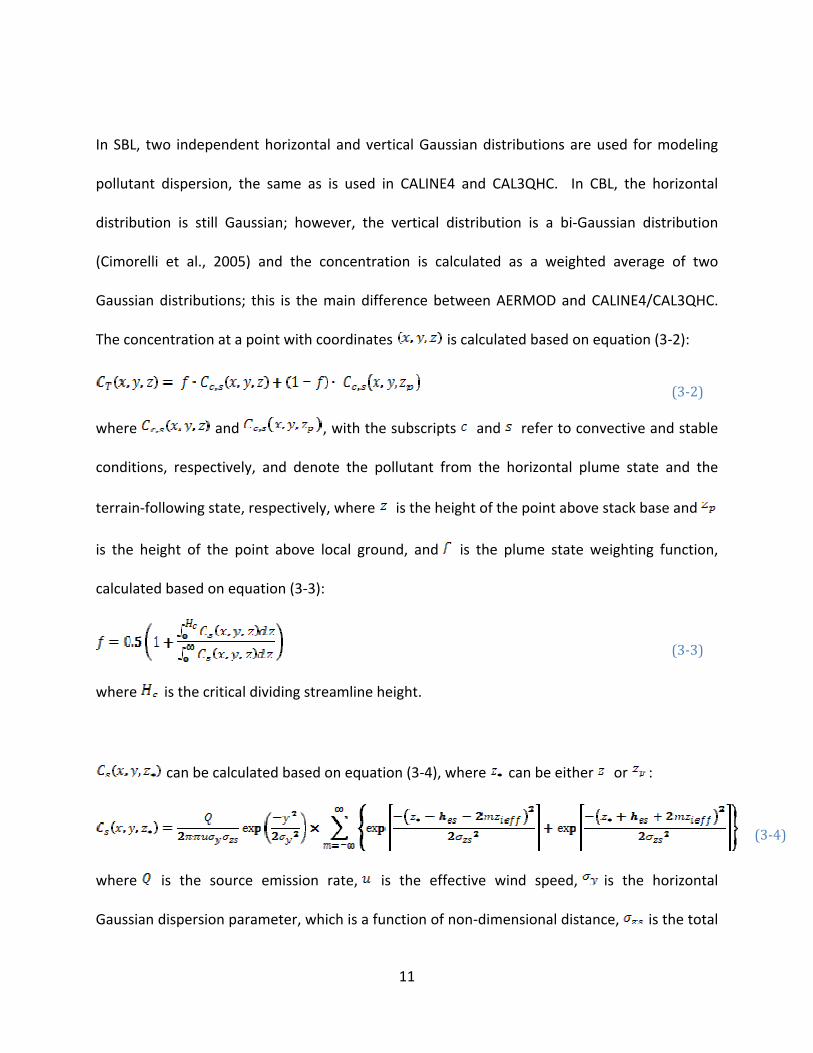
The concentration at a point with coordinates is calculated based on equation (3‐2):

(3‐2)where and , with the subscripts and refer to convective and stable

conditions, respectively, and denote the pollutant from the horizontal plume state and the

terrain‐following state, respectively, where is the height of the point above stack base and

is the height of the point above local ground, and is the plume state weighting function,

calculated based on equation (3‐3):

(3‐3)where is the critical dividing streamline height.

can be calculated based on equation (3‐4), where can be either or :

(3‐4)

where is the source emission rate, is the effective wind speed, is the horizontal

Gaussian dispersion parameter, which is a function of non‐dimensional distance, is the total

12

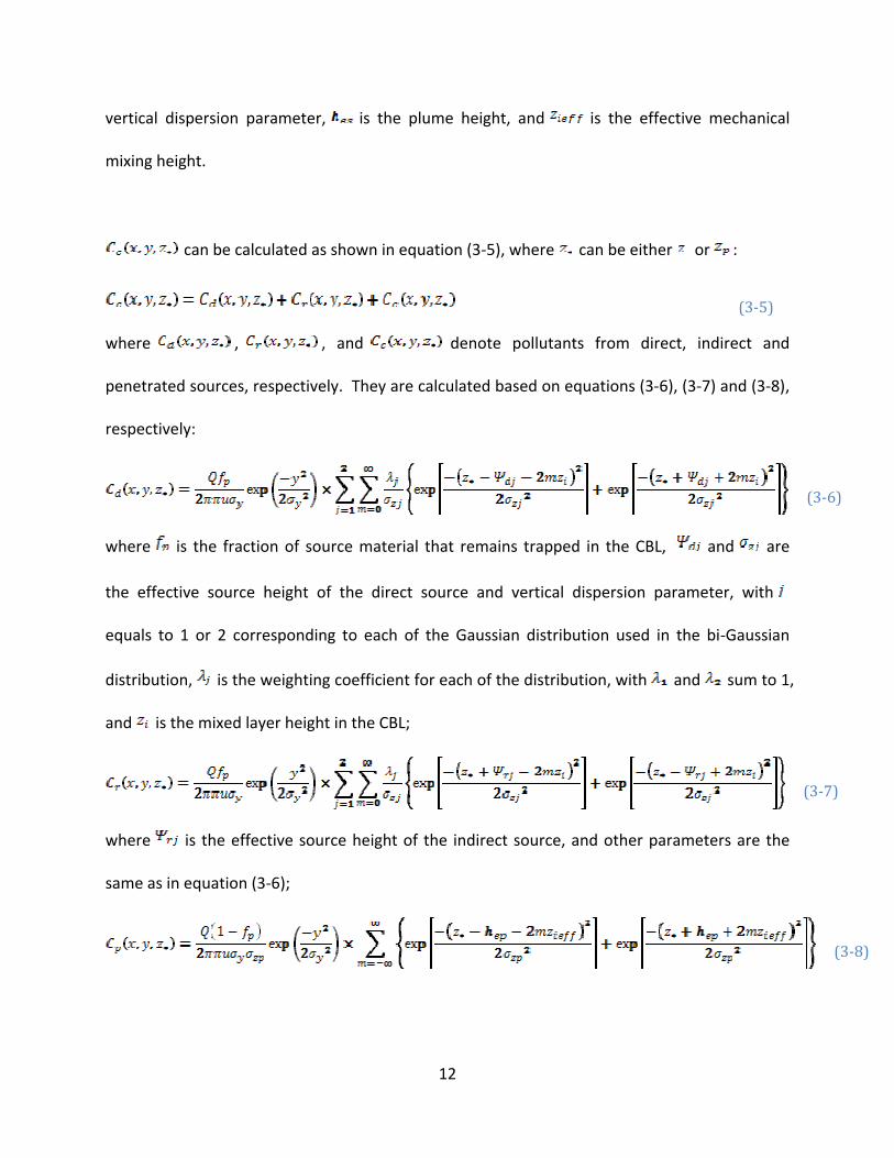
vertical dispersion parameter, is the plume height, and is the effective mechanical

mixing height.

can be calculated as shown in equation (3‐5), where can be either or :

(3‐5)where , , and denote pollutants from direct, indirect and

penetrated sources, respectively. They are calculated based on equations (3‐6), (3‐7) and (3‐8),

respectively:

(3‐6)

where is the fraction of source material that remains trapped in the CBL, and are

the effective source height of the direct source and vertical dispersion parameter, with

equals to 1 or 2 corresponding to each of the Gaussian distribution used in the bi‐Gaussian

distribution, is the weighting coefficient for each of the distribution, with and sum to 1,

and is the mixed layer height in the CBL;

(3‐7)

where is the effective source height of the indirect source, and other parameters are the

same as in equation (3‐6);

(3‐8)

13

where is the vertical dispersion coefficient, is the source height of the penetrated

source, and other parameters the same as in equations (3‐4) and (3‐6).

3.4 Data Requirements

To estimate near‐road PM2.5 concentrations, all three models need vehicle‐related data,

meteorological information and data such as link geometry and receptor locations (see Table 3‐

1). Vehicle‐related data mainly include traffic volumes and vehicle emission factors. They are

used as direct inputs in CALINE4 and CAL3QHC, and they are used to calculate source emission

rates together with source type and geometry information in AERMOD. CAL3QHC has a queue

algorithm as an optional function, which requires additional traffic data.

CALINE4 and CAL3QHC have almost the same requirements for meteorological data, while

AERMOD requires much more detailed meteorological information. For example, AERMOD

requires upper air sounding data including atmospheric pressure, dry bulb temperature, dew‐

point temperature, and wind direction and wind speed at several levels above sea level. Ideally,

when ample meteorological data are available, AERMOD may replicate atmospheric conditions

better than CALINE4 or CAL3QHC. However, AERMOD also increases the complexity of model

runs and parameter specifications due to relatively intensive data needs.

14

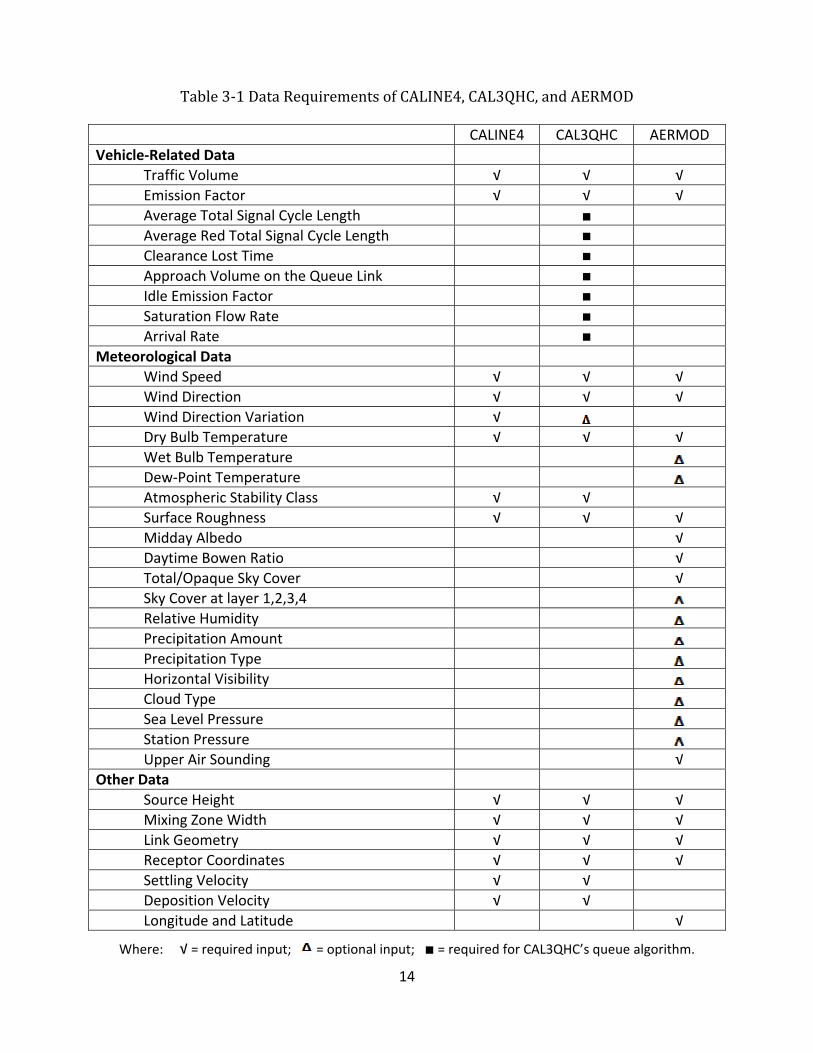
Table 3‐1 Data Requirements of CALINE4, CAL3QHC, and AERMOD

Where: √ = required input; = optional input; ■ = required for CAL3QHC’s queue algorithm.

CALINE4 CAL3QHC AERMOD Vehicle‐Related Data

Traffic Volume √ √ √ Emission Factor √ √ √ Average Total Signal Cycle Length ■ Average Red Total Signal Cycle Length ■ Clearance Lost Time ■ Approach Volume on the Queue Link ■ Idle Emission Factor ■ Saturation Flow Rate ■ Arrival Rate ■

Meteorological Data Wind Speed √ √ √ Wind Direction √ √ √ Wind Direction Variation √ Dry Bulb Temperature √ √ √ Wet Bulb Temperature Dew‐Point Temperature Atmospheric Stability Class √ √ Surface Roughness √ √ √ Midday Albedo √ Daytime Bowen Ratio √ Total/Opaque Sky Cover √ Sky Cover at layer 1,2,3,4 Relative Humidity Precipitation Amount Precipitation Type Horizontal Visibility Cloud Type Sea Level Pressure Station Pressure Upper Air Sounding √

Other Data Source Height √ √ √ Mixing Zone Width √ √ √ Link Geometry √ √ √ Receptor Coordinates √ √ √ Settling Velocity √ √ Deposition Velocity √ √ Longitude and Latitude √

15

4 Case Study – Background and Model Setup

4.1 Study Area

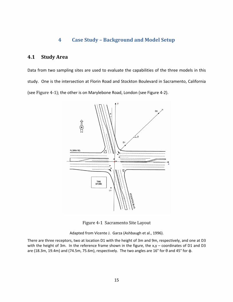
Data from two sampling sites are used to evaluate the capabilities of the three models in this

study. One is the intersection at Florin Road and Stockton Boulevard in Sacramento, California

(see Figure 4‐1); the other is on Marylebone Road, London (see Figure 4‐2).

Figure 4‐1 Sacramento Site Layout

Adapted from Vicente J. Garza (Ashbaugh et al., 1996). There are three receptors, two at location D1 with the height of 3m and 9m, respectively, and one at D3 with the height of 3m. In the reference frame shown in the figure, the x,y – coordinates of D1 and D3 are (18.3m, 19.4m) and (74.5m, 75.6m), respectively. The two angles are 16° for θ and 45° for φ.

16

Florin Road has seven lanes and its width is 26m. Stockton Boulevard has six lanes and its width

is 22m. Both links extended 150m (Ashbaugh et al., 1996) from the center of the intersection

and are considered in the model analyses, i.e., two links of 300m. By convention, if there is no

immediate barrier at sides of the road, the region within 3m at each side of the road is also

considered as the emission source (Benson, 1984, pp.160). Therefore, two rectangles are

considered as sources in this situation. The area of the Florin Road rectangle is 300m times

32m, with the coordinates of the four corners being (‐150m, ‐16m), (‐150m, 16m), (150m, 16m)

and (150m, ‐16m). The area of the Stockton Boulevard rectangle is 300m times 28m, with the

coordinates of the four corners (‐27.9m, 148.0m), (‐54.8m, 140.3m), (27.9m, ‐148.0m) and

(55.8m, ‐140.3m) (see reference x‐y axis frame shown in Figure 4‐1).

17

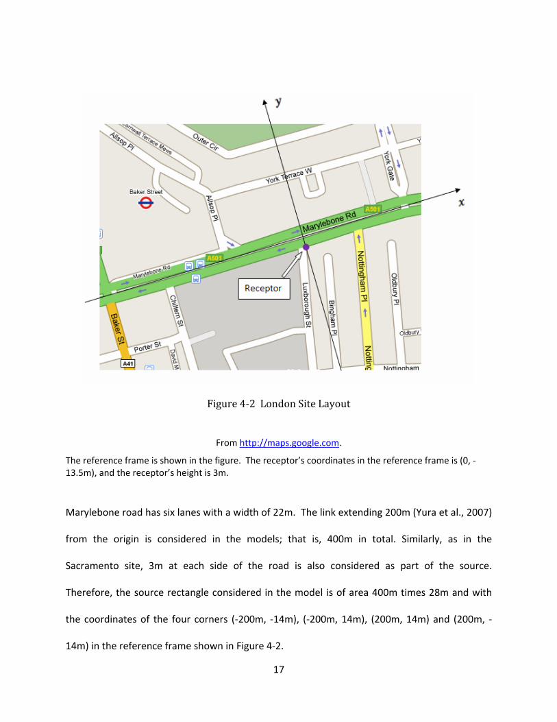
Figure 4‐2 London Site Layout

From http://maps.google.com.

The reference frame is shown in the figure. The receptor’s coordinates in the reference frame is (0, ‐13.5m), and the receptor’s height is 3m.

Marylebone road has six lanes with a width of 22m. The link extending 200m (Yura et al., 2007)

from the origin is considered in the models; that is, 400m in total. Similarly, as in the

Sacramento site, 3m at each side of the road is also considered as part of the source.

Therefore, the source rectangle considered in the model is of area 400m times 28m and with

the coordinates of the four corners (‐200m, ‐14m), (‐200m, 14m), (200m, 14m) and (200m, ‐

14m) in the reference frame shown in Figure 4‐2.

18

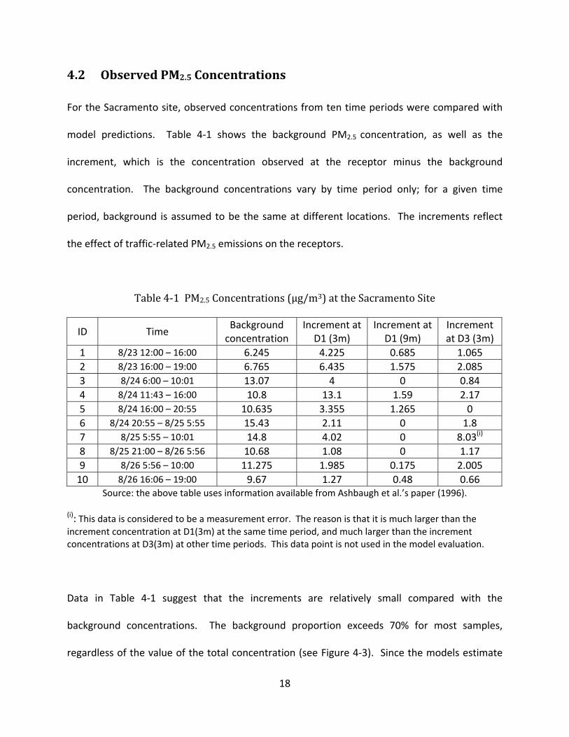
4.2 Observed PM2.5 Concentrations

For the Sacramento site, observed concentrations from ten time periods were compared with

model predictions. Table 4‐1 shows the background PM2.5 concentration, as well as the

increment, which is the concentration observed at the receptor minus the background

concentration. The background concentrations vary by time period only; for a given time

period, background is assumed to be the same at different locations. The increments reflect

the effect of traffic‐related PM2.5 emissions on the receptors.

Table 4‐1 PM2.5 Concentrations (µg/m3) at the Sacramento Site ID Time

Background concentration

Increment at D1 (3m)

Increment at D1 (9m)

Increment at D3 (3m)

1 8/23 12:00 – 16:00 6.245 4.225 0.685 1.065 2 8/23 16:00 – 19:00 6.765 6.435 1.575 2.085 3 8/24 6:00 – 10:01 13.07 4 0 0.84 4 8/24 11:43 – 16:00 10.8 13.1 1.59 2.17 5 8/24 16:00 – 20:55 10.635 3.355 1.265 0 6 8/24 20:55 – 8/25 5:55 15.43 2.11 0 1.8 7 8/25 5:55 – 10:01 14.8 4.02 0 8.03(i) 8 8/25 21:00 – 8/26 5:56 10.68 1.08 0 1.17 9 8/26 5:56 – 10:00 11.275 1.985 0.175 2.005

10 8/26 16:06 – 19:00 9.67 1.27 0.48 0.66 Source: the above table uses information available from Ashbaugh et al.’s paper (1996).

(i): This data is considered to be a measurement error. The reason is that it is much larger than the increment concentration at D1(3m) at the same time period, and much larger than the increment concentrations at D3(3m) at other time periods. This data point is not used in the model evaluation.

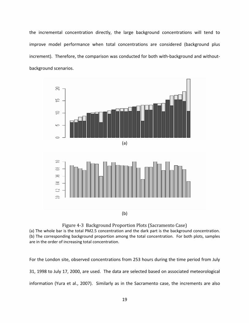
Data in Table 4‐1 suggest that the increments are relatively small compared with the

background concentrations. The background proportion exceeds 70% for most samples,

regardless of the value of the total concentration (see Figure 4‐3). Since the models estimate

19

the incremental concentration directly, the large background concentrations will tend to

improve model performance when total concentrations are considered (background plus

increment). Therefore, the comparison was conducted for both with‐background and without‐

background scenarios.

(a)

(b) Figure 4‐3 Background Proportion Plots (Sacramento Case)

(a) The whole bar is the total PM2.5 concentration and the dark part is the background concentration. (b) The corresponding background proportion among the total concentration. For both plots, samples are in the order of increasing total concentration.

For the London site, observed concentrations from 253 hours during the time period from July

31, 1998 to July 17, 2000, are used. The data are selected based on associated meteorological

information (Yura et al., 2007). Similarly as in the Sacramento case, the increments are also

20

relatively small when compared with the background concentrations. Therefore, as with the

Sacramento case study, concentrations with and without background are considered in the

model comparisons.

4.3 Model Inputs

Because detailed intersection information (e.g., signal data, idling emissions, and traffic delays)

is unavailable for both sites, the queuing algorithm embedded in the CAL3QHC model was not

used. In addition, AERMOD was not used for the London site, because upper air sounding data

and sky cover information were lacking for the monitoring events.

The surface roughness is set to be 100cm for both sites since they are in urban areas. The

midday Albedo and daytime Bowen ratio required for AERMOD are set to be 0.16 and 2.0,

respectively, according to AERMOD’s User Guideline (USEPA, 2004c). Two important

parameters are discussed below.

4.3.1 Emission Factor (EF)

Two methods were used for quantifying emission factors. In the Sacramento case, a steady‐

state box model was used. The model assumes a virtual box over the road segment and the

pollutant concentration is uniform inside the box. The emission factor is calculated as shown in

equation (4‐1):

21

(4‐1)where is the wind speed (m/s), is the height of the mixing box (m), is the measured

pollutant concentration (µg/m3), is the wind direction (degrees), is the number of vehicles

per hour, and the calculated emission factor is of the unit of gram per vehicle kilometer

traveled (g/VKT) (Ashbaugh et al., 1996). The box model is used in the Sacramento case so that

the calculated emission factors reflect both free‐flow and idling vehicle emissions.

In the London site, the emission factor is calculated as a weighted average over different

vehicle categories as shown in equation (4‐2). The emission factors of light‐duty vehicles and

heavy‐duty vehicles are shown in Table 4‐2:

(4‐2)where the subscripts and denote ‘light‐duty vehicle’ and ‘heavy‐duty vehicle’,

respectively, and is the vehicle number.

Table 4‐2 Emission factors of PM2.5 (g/VKT) Year 1998 1999 2000

Light‐duty vehicle 0.0268 0.0260 0.0225 Heavy‐duty vehicle 0.418 0.358 0.279

Source: (Yura et al., 2007).

22

4.3.2 Deposition and Settling Velocities

PM2.5 can be removed from the atmosphere by dry deposition, precipitation scavenging, and/or

chemical reactions. In both case studies, models are used on days without precipitation and we

also do not consider the chemical reactions of PM2.5; only dry deposition is considered.

Dry deposition is mainly due to gravitation, turbulent diffusion and Brownian motion (Hanna et

al., 1982, pp 67‐71). By Stokes’ law, the terminal settling speed ( ), which is due to gravitation,

can be calculated based on equation (4‐3):

(4‐3) where is the particle radii, is particle density, and is dynamic viscosity of air

( ). In the two case studies, the concentration of PM2.5 is estimated, so

the particle radii is no more than 1.25 µm, also the particle densities are no more than 60

µg/m3 in both case studies, so the calculated terminal settling speed is no more than

, which is very small and is negligible. The dry deposition by turbulent

diffusion and Brownian motion are also negligible because of the low particle densities.

Therefore, the deposition velocity and settling velocity are set to be 0 as model inputs.

23

5 Case Study – Results and Analysis

Model estimations from CALINE4, CAL3QHC and AERMOD at the Sacramento site, and from

CALINE4 and CAL3QHC at the London site, were compared with measured concentrations. In

order to see how the models performed, screen plots and statistical tests were used. For the

sake of convenience, let (where represents the model: 1 – CALINE4, 2 – CAL3QHC, and 3 –

AERMOD; and is the sample ID, ) denote the difference between the model‐

predicted concentrations and the observed concentrations.

5.1 Screen Plots and Descriptive Statistics

5.1.1 Factor-of-Two Plots

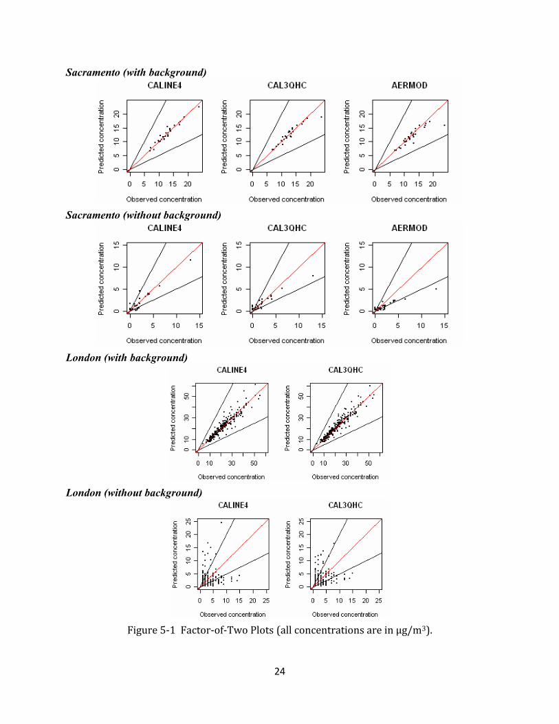
The “Factor‐of‐two” plot is a classical method to examine model performance. Typically, if 80%

of the points fall inside the factor‐of‐two envelope, the model results are considered good in

predicting true values (Yura et al., 2007, pp.8752).

Figure 5‐1 and Table 5‐1 show that all points are inside the factor‐of‐two envelope for both

Sacramento and London sites when the background concentrations are included. However,

when the background concentrations are not included, approximately half of the points are

outside the factor‐of‐two envelope, suggesting that model results with CALINE4 and CAL3QHC

do not match observed increments well, especially for the London site.

24

Sacramento (with background)

Sacramento (without background)

London (with background)

London (without background)

Figure 5‐1 Factor‐of‐Two Plots (all concentrations are in µg/m3).

25

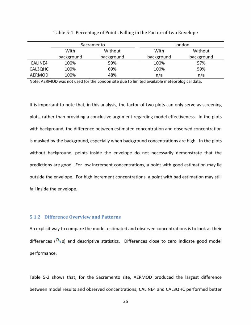
Table 5‐1 Percentage of Points Falling in the Factor‐of‐two Envelope Sacramento London

With

background Without

background With

background Without

background CALINE4 100% 59% 100% 57% CAL3QHC 100% 69% 100% 59% AERMOD 100% 48% n/a n/a Note: AERMOD was not used for the London site due to limited available meteorological data.

It is important to note that, in this analysis, the factor‐of‐two plots can only serve as screening

plots, rather than providing a conclusive argument regarding model effectiveness. In the plots

with background, the difference between estimated concentration and observed concentration

is masked by the background, especially when background concentrations are high. In the plots

without background, points inside the envelope do not necessarily demonstrate that the

predictions are good. For low increment concentrations, a point with good estimation may lie

outside the envelope. For high increment concentrations, a point with bad estimation may still

fall inside the envelope.

5.1.2 Difference Overview and Patterns

An explicit way to compare the model‐estimated and observed concentrations is to look at their

differences ( s) and descriptive statistics. Differences close to zero indicate good model

performance.

Table 5‐2 shows that, for the Sacramento site, AERMOD produced the largest difference

between model results and observed concentrations; CALINE4 and CAL3QHC performed better

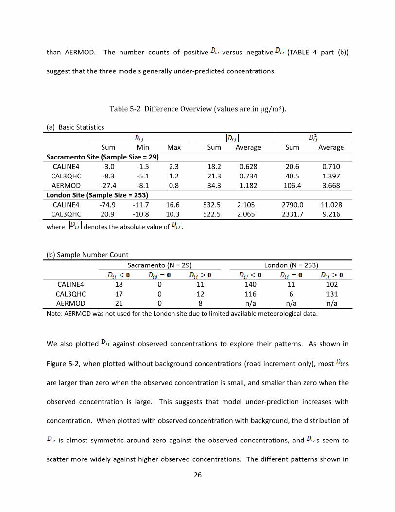
26

than AERMOD. The number counts of positive versus negative (TABLE 4 part (b))

suggest that the three models generally under‐predicted concentrations.

Table 5‐2 Difference Overview (values are in µg/m3). (a) Basic Statistics

Sum Min Max Sum Average Sum Average

Sacramento Site (Sample Size = 29) CALINE4 ‐3.0 ‐1.5 2.3 18.2 0.628 20.6 0.710 CAL3QHC ‐8.3 ‐5.1 1.2 21.3 0.734 40.5 1.397 AERMOD ‐27.4 ‐8.1 0.8 34.3 1.182 106.4 3.668

London Site (Sample Size = 253) CALINE4 ‐74.9 ‐11.7 16.6 532.5 2.105 2790.0 11.028 CAL3QHC 20.9 ‐10.8 10.3 522.5 2.065 2331.7 9.216

where denotes the absolute value of . (b) Sample Number Count

Sacramento (N = 29) London (N = 253)

CALINE4 18 0 11 140 11 102 CAL3QHC 17 0 12 116 6 131 AERMOD 21 0 8 n/a n/a n/a

Note: AERMOD was not used for the London site due to limited available meteorological data.

We also plotted against observed concentrations to explore their patterns. As shown in

Figure 5‐2, when plotted without background concentrations (road increment only), most s

are larger than zero when the observed concentration is small, and smaller than zero when the

observed concentration is large. This suggests that model under‐prediction increases with

concentration. When plotted with observed concentration with background, the distribution of

is almost symmetric around zero against the observed concentrations, and s seem to

scatter more widely against higher observed concentrations. The different patterns shown in

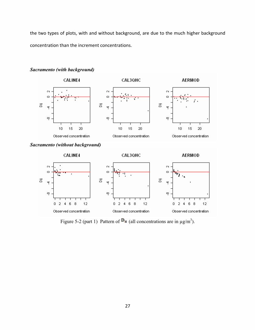
27

the two types of plots, with and without background, are due to the much higher background

concentration than the increment concentrations.

Sacramento (with background)

Sacramento (without background)

Figure 5-2 (part 1) Pattern of (all concentrations are in µg/m3).

28

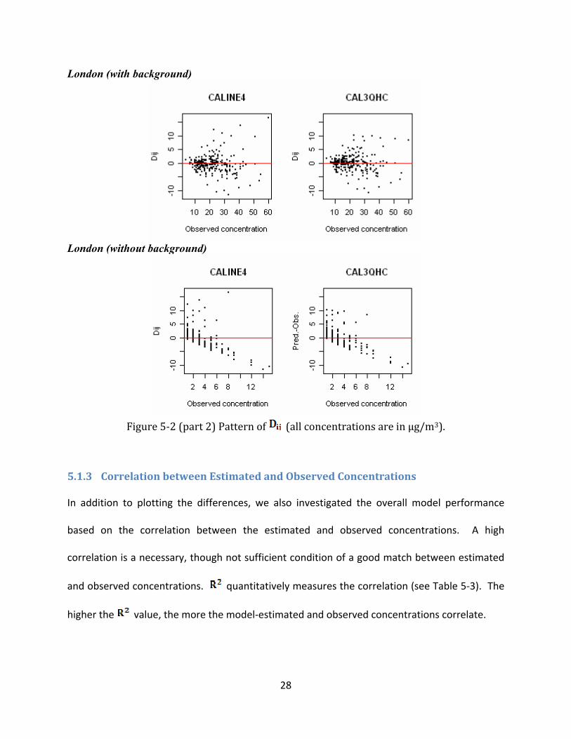
London (with background)

London (without background)

Figure 5‐2 (part 2) Pattern of (all concentrations are in µg/m3).

5.1.3 Correlation between Estimated and Observed Concentrations

In addition to plotting the differences, we also investigated the overall model performance

based on the correlation between the estimated and observed concentrations. A high

correlation is a necessary, though not sufficient condition of a good match between estimated

and observed concentrations. quantitatively measures the correlation (see Table 5‐3). The

higher the value, the more the model‐estimated and observed concentrations correlate.

29

Table 5‐3 R2 correlating model‐predicted and observed concentrations. Sacramento London

With

background Without

background With

background Without

background CALINE4 0.9454 0.8952 0.9009 0.0277 CAL3QHC 0.9044 0.8973 0.9134 0.0329 AERMOD 0.7905 0.8513 n/a n/a Note: AERMOD was not used for the London site due to limited available meteorological data.

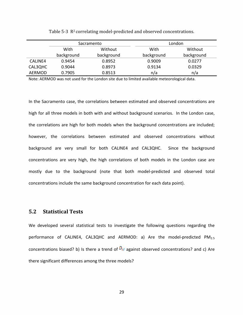
In the Sacramento case, the correlations between estimated and observed concentrations are

high for all three models in both with and without background scenarios. In the London case,

the correlations are high for both models when the background concentrations are included;

however, the correlations between estimated and observed concentrations without

background are very small for both CALINE4 and CAL3QHC. Since the background

concentrations are very high, the high correlations of both models in the London case are

mostly due to the background (note that both model‐predicted and observed total

concentrations include the same background concentration for each data point).

5.2 Statistical Tests

We developed several statistical tests to investigate the following questions regarding the

performance of CALINE4, CAL3QHC and AERMOD: a) Are the model‐predicted PM2.5

concentrations biased? b) Is there a trend of against observed concentrations? and c) Are

there significant differences among the three models?

30

5.2.1 Test of Prediction Bias

We used the one‐sample t‐test to examine the hypothesis that the predicted concentrations

provided by the three models are not biased. In order to perform the test, an assumption is

made for that (N is the sample size) are samples from a population with one

distribution. As long as N is larger than 29, the central limit theorem can be applied and the

one‐sample t‐test can be conducted. Both test statistic and p‐value are calculated. A criterion

of 0.05 for p‐value is used; that is, if the p‐value is smaller than 0.05, then we reject the

hypothesis (i.e., the model is biased). In this particular case, we can also determine whether

the model is under or over‐predicting based on the sign of the test statistic. If the hypothesis is

rejected, then a negative test statistic indicates under‐predicting, while a positive test statistic

suggests over‐predicting.

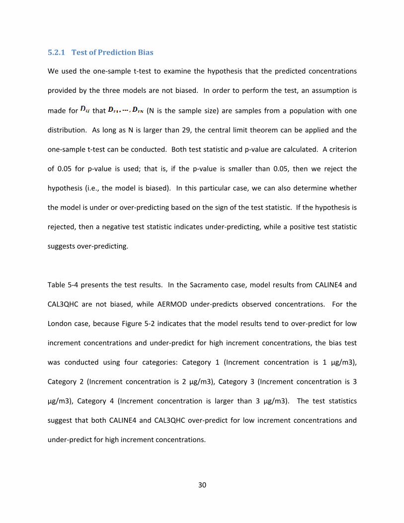
Table 5‐4 presents the test results. In the Sacramento case, model results from CALINE4 and

CAL3QHC are not biased, while AERMOD under‐predicts observed concentrations. For the

London case, because Figure 5‐2 indicates that the model results tend to over‐predict for low

increment concentrations and under‐predict for high increment concentrations, the bias test

was conducted using four categories: Category 1 (Increment concentration is 1 µg/m3),

Category 2 (Increment concentration is 2 µg/m3), Category 3 (Increment concentration is 3

µg/m3), Category 4 (Increment concentration is larger than 3 µg/m3). The test statistics

suggest that both CALINE4 and CAL3QHC over‐predict for low increment concentrations and

under‐predict for high increment concentrations.

31

Table 5‐4 Test Results for Prediction Bias. (a) Sacramento Case (N = 29)

‐value Conclusion CALINE4 ‐0.6643 0.512 Unbiased CAL3QHC ‐1.3281 0.195 Unbiased AERMOD ‐3.0004 0.0056 Under‐Prediction (b) London Case

Category 1 (N = 74) Category 2 (N = 58) ‐value Conclusion ‐value Conclusion

CALINE4 5.353 <0.0001 Over‐Prediction 1.354 0.181 Unbiased CAL3QHC 7.236 <0.0001 Over‐Prediction 2.998 0.004 Over‐Prediction

Category 3 (N = 53) Category 4 (N = 68) CALINE4 ‐0.302 0.764 Unbiased ‐5.192 <0.0001 Under‐Prediction CAL3QHC 0.761 0.450 Unbiased ‐5.461 <0.0001 Under‐Prediction Category 1 (Increment concentration is 1 µg/m3), Category 2 (Increment concentration is 2 µg/m3), Category 3 (Increment concentration is 3 µg/m3), Category 4 (Increment concentration is larger than 3 µg/m3).

5.2.2 Test of Prediction Trend

We conducted an alternate statistical test to explore the statistical significance of the trend that

model under‐prediction increases with increased concentration (i.e., decrease with

increasing increment concentrations, as shown in Figure 5‐2). The hypothesis is that the slope

of the regression between and the observed concentration is zero. If the test shows that

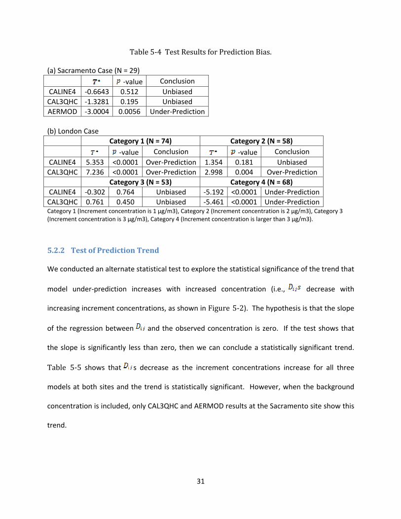
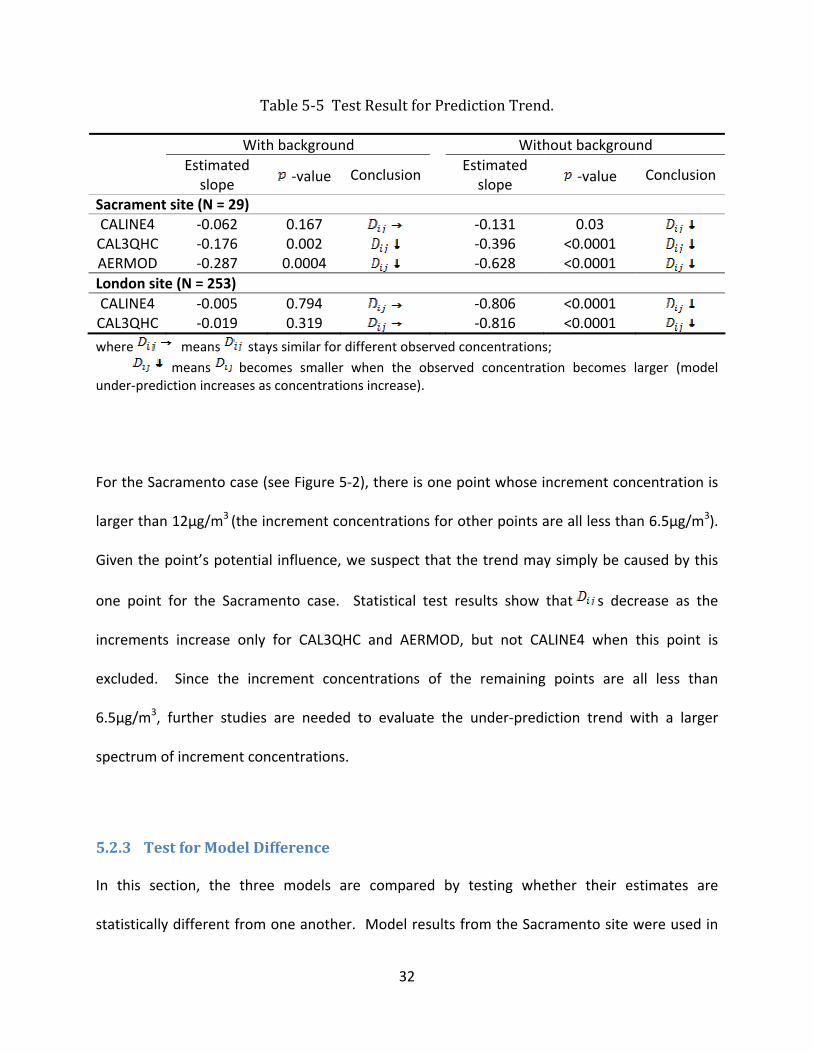
the slope is significantly less than zero, then we can conclude a statistically significant trend. Table 5‐5 shows that s decrease as the increment concentrations increase for all three

models at both sites and the trend is statistically significant. However, when the background

concentration is included, only CAL3QHC and AERMOD results at the Sacramento site show this

trend.

32

Table 5‐5 Test Result for Prediction Trend. With background Without background

Estimated slope ‐value Conclusion

Estimated slope ‐value Conclusion

Sacrament site (N = 29) CALINE4 ‐0.062 0.167 ‐0.131 0.03 CAL3QHC ‐0.176 0.002 ‐0.396 <0.0001 AERMOD ‐0.287 0.0004 ‐0.628 <0.0001 London site (N = 253) CALINE4 ‐0.005 0.794 ‐0.806 <0.0001 CAL3QHC ‐0.019 0.319 ‐0.816 <0.0001 where means stays similar for different observed concentrations; means becomes smaller when the observed concentration becomes larger (model under‐prediction increases as concentrations increase).

For the Sacramento case (see Figure 5‐2), there is one point whose increment concentration is

larger than 12µg/m3 (the increment concentrations for other points are all less than 6.5µg/m3).

Given the point’s potential influence, we suspect that the trend may simply be caused by this

one point for the Sacramento case. Statistical test results show that s decrease as the

increments increase only for CAL3QHC and AERMOD, but not CALINE4 when this point is

excluded. Since the increment concentrations of the remaining points are all less than

6.5µg/m3, further studies are needed to evaluate the under‐prediction trend with a larger

spectrum of increment concentrations.

5.2.3 Test for Model Difference

In this section, the three models are compared by testing whether their estimates are

statistically different from one another. Model results from the Sacramento site were used in

33

this test and a one‐factor ANOVA model was constructed. The ANOVA model specified s as

the sample results and included one factor with three levels representing the three models

(level 1 ‐ CALINE4, level 2 ‐ CAL3QHC, and level 3 ‐ AERMOD). The sample size for each factor

level is 29.

A hypothesis that the three models are not different from each other can be tested through a

simultaneous 95% confidence interval for the three combinations of the differences between

means of the three factor levels, , , and , where , and are the

means of factor level 1, 2 and 3, respectively. Using the Bonferroni method, we can get

confidence intervals between means of factor levels:

: [‐0.642, 1.008]

: [0.015, 1.665]

: [‐0.168, 1.482]

Since both bounds of the interval of are positive, the test suggests that predicted

concentrations from AERMOD are significantly smaller than those provided by CALINE4 at the

Sacramento site. This is consistent with the evidence in section 5.2.1 that AERMOD under‐

predicts PM2.5 concentrations. The interval of is almost symmetric around 0, which

indicates that CALINE4 and CAL3QHC produce concentration estimates that are not statistically

different from each other.

34

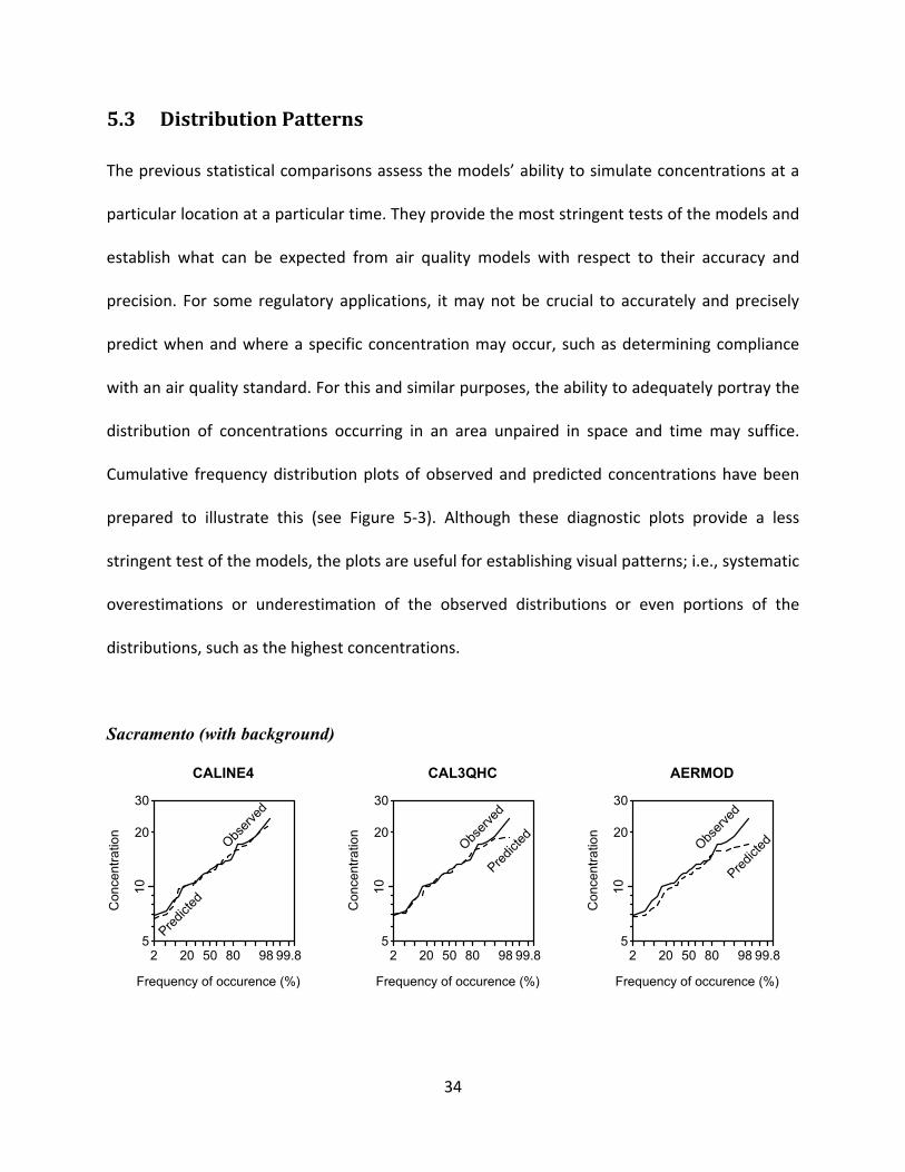
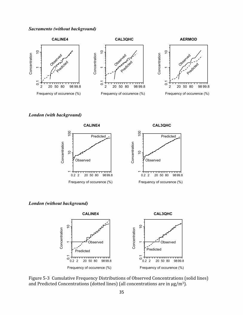
5.3 Distribution Patterns

The previous statistical comparisons assess the models’ ability to simulate concentrations at a

particular location at a particular time. They provide the most stringent tests of the models and

establish what can be expected from air quality models with respect to their accuracy and

precision. For some regulatory applications, it may not be crucial to accurately and precisely

predict when and where a specific concentration may occur, such as determining compliance

with an air quality standard. For this and similar purposes, the ability to adequately portray the

distribution of concentrations occurring in an area unpaired in space and time may suffice.

Cumulative frequency distribution plots of observed and predicted concentrations have been

prepared to illustrate this (see Figure 5‐3). Although these diagnostic plots provide a less

stringent test of the models, the plots are useful for establishing visual patterns; i.e., systematic

overestimations or underestimation of the observed distributions or even portions of the

distributions, such as the highest concentrations.

Sacramento (with background)

2 20 50 80 98 99.8

Frequency of occurence (%)

10

20

30

5

Con

cent

ratio

n

CALINE4

Observ

ed

Predict

ed

2 20 50 80 98 99.8

Frequency of occurence (%)

10

20

30

5

Con

cent

ratio

n

CAL3QHC

Observ

ed

Predict

ed

2 20 50 80 98 99.8

Frequency of occurence (%)

10

20

30

5

Con

cent

ratio

n

AERMOD

Observ

ed

Predict

ed

35

Sacramento (without background)

2 20 50 80 98 99.8

Frequency of occurence (%)

0.1

110

Con

cent

ratio

n

CALINE4

Observ

ed

Predict

ed

2 20 50 80 98 99.8

Frequency of occurence (%)

0.1

110

Con

cent

ratio

n

CAL3QHC

Observ

ed

Predict

ed

2 20 50 80 98 99.8

Frequency of occurence (%)

0.1

110

Con

cent

ratio

n

AERMOD

Observ

ed

Predict

ed

London (with background)

0.2 2 20 50 80 9899.8

Frequency of occurence (%)

110

100

Con

cent

ratio

n

CALINE4

Predicted

Observed

0.2 2 20 50 80 9899.8

Frequency of occurence (%)

110

100

Con

cent

ratio

n

CAL3QHC

Predicted

Observed

London (without background)

0.2 2 20 50 80 9899.8

Frequency of occurence (%)

0.1

110

Con

cent

ratio

n

CALINE4

Predicted

Observed

0.2 2 20 50 80 9899.8

Frequency of occurence (%)

0.1

110

Con

cent

ratio

n

CAL3QHC

Predicted

Observed

Figure 5‐3 Cumulative Frequency Distributions of Observed Concentrations (solid lines) and Predicted Concentrations (dotted lines) (all concentrations are in µg/m3).

36

6 Discussion and Conclusion

In this study, when comparing predicted and observed concentrations, scenarios with and

without background are considered. Screen plots and statistical tests show that different

results may be concluded from the two scenarios.

In the Sacramento case, model results paired in space and time from CALINE4 and CAL3QHC

match the observed concentrations moderately well, while AERMOD under‐predicts PM2.5

concentrations, based on a prediction bias test (section 5.2.1) and confidence intervals of the

difference between means (section 5.2.3). All three models show a trend of under‐predicting

the observed values as the increment concentrations increase (section 5.2.2). When the data

point with an increment concentration of 12µg/m3 is excluded (all remaining data points are of

increment concentrations less than 6.5µg/m3), statistical test results show that s decrease as

the increments increase only for CAL3QHC and AERMOD, but not for CALINE4. Therefore,

further studies are needed to investigate how well the models perform across a larger

spectrum of road‐increment PM2.5 concentrations.

In the London case, model results paired in space and time from CALINE4 and CAL3QHC do not

match the observed concentrations (increments, without background). When the increment

concentrations are small, both models over‐predicted; for high increment concentrations, both

models under‐predicted. Both models showed a trend of predicting smaller than monitored

values as the increment concentrations increased. In addition, when the backgrounds are

37

excluded, the predicted concentrations behave as randomly chosen numbers against the

observed concentration. The values also show little correlation between model results and

measured concentrations when the backgrounds are excluded. There are two possible reasons

for this bad match. First, the receptor at the London site is very close to the road segment. It is

highly affected by instant nearby traffic and meteorological conditions. However, both models

assume that the point for which the concentration is estimated achieves a steady state. This

assumption is therefore not satisfied for the receptor location at the London site. Second, the

street canyon effect may play an important role in PM dispersion at the London site. Since the

study site includes numerous high buildings, the street canyon effect results in complex

meteorology near the receptor. The comparison of London’s results therefore indicates that

CALINE4 and CAL3QHC are not suitable for estimating concentrations at places where stable

state is not achieved.

Our comparative assessment suggests that AERMOD under‐estimates near‐road PM2.5

concentrations at the Sacramento site. This is consistent with two previous studies that have

shown under‐predicted PM10 concentrations in AERMOD (Kesarkar et al., 2007; Zhang et al.,

2008). Prior works, together with these findings, suggest that AERMOD may be inappropriate

for estimating PM concentrations near roads. The evidence that AERMOD appears to under‐

predict concentrations, combined with the fact that more meteorological data and more user

effort is required to run AERMOD, suggest that project‐level analysts may want to run either

CALINE4 or CAL3QHC as a first choice.

38

Note also, that theoretically, AERMOD can mimic real atmospheric conditions better; however,

it requires more meteorological data to run, some of which can be difficult to obtain. (In the

London case, AERMOD was not run because of limited available meteorological data.)

Moreover, running AERMOD requires more user effort than the other two models due to the

complexity of the model.

CAL3QHC has an optional queue algorithm. Using this algorithm may better simulate vehicle

movements in signalized road segments. However, signal‐related parameters and idle emission

factors are needed in order to make use of the queue algorithm. In many cases, it is not easy to

specify these parameters.

Another implication from this study is that factor‐of‐two plots are a limited resource for model

evaluation. Factor‐of‐two plots have been a traditional test of model performance, and several

previous studies have assessed model performance based solely or largely on the percentage of

data points falling inside the factor‐of‐two envelope. As shown by this study, factor‐of‐two

plots assist in screening‐level assessments but lack the statistical detail offered by other tests.

Both the CALINE4 and CAL3QHC models accurately simulate the distribution of observed

concentrations at the Sacramento and London sites. In the less rigorous comparison of

predicted and observed concentrations unpaired in space and time, quite an improvement in

model performances are indicated for the London site, with a slight advantage exhibited by the

CAL3QHC model. Modelers should keep in mind, however, that this represents a compromised

39

application case, where it is not important to determine when and where a specific

concentration may occur. AERMOD tended to under‐predict observed concentrations

throughout most of the distribution as reflected in the statistical comparisons.

40

References

Abdul‐Wahab, S. A. (2004). An application and evaluation of the CAL3QHC model for predicting carbon monoxide concentrations from motor vehicles near a roadway intersection in Muscat, Oman. Environmental Management 34, 372‐382.

Adar, S. D., Gold, D. R., Coull, B. A., Schwartz, J., Stone, P. H., and Suh, H. (2007). Focused Exposures to Airborne Traffic Particles and Heart Rate Variability in the Elderly. Epidemiology 18, 95‐103.

Ashbaugh, L. L., Flocchini, R. G., Chang, D., Carvacho, O. F., James, T. A., and Matsumura, R. T. (1996). Final Report: Traffic Generated PM10 "Hot Spots". Caltrans Contract No. 53V606 A2.

Benson, P. E. (1984). CALINE4 ‐ A dispersion model for predicting air pollutant concentrations near roadways. FHWA/CA/TL‐84/15.

Benson, P. E. (1992). A REVIEW OF THE DEVELOPMENT AND APPLICATION OF THE CALINE3 AND CALINE4 MODELS Atmospheric Environment Part B‐Urban Atmosphere 26, 379‐390

Bowker, G. E., Baldauf, R., Isakov, V., Khlystov, A., and Petersen, W. (2007). The effects of roadside structures on the transport and dispersion of ultrafine particles from highways. Atmospheric Environment 41, 8128‐8139.

Broderick, B. M., Budd, U., and Misstear, B. D. (2005). Validation of CALINE4 modelling for carbon monoxide concentrations under free‐flowing and congested traffic conditions in Ireland. International Journal of Environment and Pollution 24, 104‐113.

Broderick, B. M., and O'Donoghue, R. T. (2007). Spatial variation of roadside C2‐C6 hydrocarbon concentrations during low wind speeds: Validation of CALINE4 and COPERT III modelling. Transportation Research Part D 12, 537‐547.

Brugge, D., Durant, J. L., and Rioux, C. (2007). Near‐Highway Pollutants in Motor Vehicle Exhaust: A Review of Epidemiologic Evidence of Cardiac and Pulmonary Health Risks. Environmental Health 6.

Carr, E. L., Johnson, R. G., and Ireson, R. G. (2002). User's Guide to HYROAD ‐ The Hybrid Roadway Intersection Model SYSAPP‐02‐073d.

Cimorelli, A. J., Perry, S. G., Venkatram, A., Weil, J. C., Paine, R. J., Wilson, R. B., Lee, R. F., Peters, W. D., and Brode, R. W. (2005). AERMOD: A Dispersion Model for Industrial Source Applications. Part I: General Model Formulation and Boundary Layer Characterization. Journal of Applied Meteorology 44, 682‐693.

Davidson, C. I., Phalen, R. F., and Solomon, P. A. (2005). Airborne Particulate Matter and Human Health: A Review. Aerosol Science and Technology 39, 737‐749.

41

Englert, N. (2004). Fine Particles and Human Health ‐ A Review of Epidemiological Studies. Toxicology Letters 149, 235‐242.

Faulkner, W. B., Powell, J. J., Lange, J. M., Shaw, B. W., Lacey, R. E., and Parnell, C. B. (2007). Comparison of dispersion models for ammonia emissions from a a ground‐level area source. American Society of Agricultural and Biological Engineers 50, 2189‐2197.

Gokhale, S., and Raokhade, N. (2008). Performance evaluation of air quality models for predicting PM10 and PM2.5 concentrations at urban traffic intersection during winter period. Science of the Total Environment 394, 9‐24.

Gramotnev, G., Brown, R., Ristovski, Z., Hitchins, J., and Morawska, L. (2003). Determination of average emission factors for vehicles on a busy road. Atmospheric Environment 37, 465‐474.

Hanna, S. R., Briggs, G. A., and Hosker, R. P. (1982). Handbook on Atmospheric Diffusion. Technical Information Center U. S. Department of Energy.

Hanna, S. R., Paine, R., Heinold, D., Kintigh, E., and Baker, D. (2006). Uncertainties in air toxics calculated by the dispersion models AERMOD and ISCST3 in the Houston ship channel area. Journal of Applied Meteorology and Climatology 46, 1372‐1382.

Holmes, N. S., and Morawska, L. (2006). A Review of Dispersion Modeling and Its Application to the Dispersion of Particles: An Overview of Different Dispersion Models Avaiable. Atmospheric Environment 40, 5902‐5928

Jampana, S. S., Kumar, A., and Varadarajan, C. (2004). Application of the United States Environmental Protection Agency's AERMOD Model to an Industrial Area. Environmental Progress 23, 12‐18.

Jerrett, M., and Finkelstein, M. (2005). Geographies of Risk in Studies Linking Chronic Air Pollution Exposure to Health Outcomes Journal of toxicology and environmental health, Part A 68, 1207‐1242.

Jones, G., Gonzalez‐Flesca, N., Sokhi, R. S., Mcdonald, T., and MA, M. (1998). Measurement and Interpretation of Concentrations of Urban Atmospheric Organic Compounds. Environmental Monitoring and Assessment 52, 107‐121.

Kappos, A. D., Bruckmann, P., Eikmann, T., Englert, N., Heinrich, U., Hoppe, P., Koch, E., Krause, G. H. M., Kreyling, W. G., Rauchfuss, K., Rombout, P., Schulz‐Klemp, V., Thiel, W. R., and Wichmann, H. E. (2004). Health Effects of Particles in Ambient Air. International Journal of Hygiene and Environmental Health 207, 399‐407.

Kenty, K. L., Poor, N. D., Kronmiller, K. G., McClenny, W., King, C., Atkeson, T., and Campbell, S. W. (2007). Application of CALINE4 to roadside NO/NO2 transformations. Atmospheric Environment 41, 4270‐4280.

Kesarkar, A. P., Dalvi, M., Kaginalkar, A., and Ojha, A. (2007). Coupling of the Weather Research and Forecasting Model with AERMOD for Pollutant Dispersion Modeling. A Case Study for PM10 Dispersion over Pune, India. Atmospheric Environment 41, 1976‐1988.

42

Kho, F. W. L., Law, P. L., Ibrahim, S. H., and Sentian, J. (2007). Carbon monoxide levels along roadway. Int. J. Environ. Sci. Tech. 4, 27‐34.

Kim, J. J., Smorodinsky, S., Lipsett, M., Singer, B. C., Hodgson, A. T., and Ostro, B. (2004). Traffic‐Related Air Pollution Near Busy Roads. American Journal of Respiratory and Critical Care Medicine 170, 520‐526.

Kok, T. M. C. M. d., Driece, h. A. L., Hogervorst, J. G. F., and Briede, J. J. (2006). Toxicological Assessment of Ambient and Traffic‐Related Particulate Matter: A Review of Recent Studies. Mutation Research 613, 103‐122.

Kumar, A., Dixit, S., Varadarajan, C., Vijayan, A., and Masuraha, A. (2006). Evaluation of the AERMOD dispersion model as a function of atmospheric stability for an urban area. Environmental Progress 25, 141‐151.

Levitin, J., Harkonen, J., Kukkonen, J., and Nikmo, J. (2005). Evaluation of the CALINE4 and CAR‐FMI models against measurements near a major road Atmospheric Environment 39, 4439‐4452

Loranger, S., Zayed, J., and Kennedy, G. (1995). Contribution of Methylcyclopentadienyl Manganese Tricarbonyl (MMT) to Atmospheric Mn Concentration Near Expressway: Dispersion Modeling Estimations. Atmospheric Environment 29, 591‐599.

Marmur, A., and Mamane, Y. (2003). Comparison and evaluation of several mobile‐source and line‐source models in Israel Transportation Research Part D‐Transport and Environment 8, 249‐265

Moseholm, L., Silva, J., and Larson, T. (1996). Forecasting Carbon Monoxide Concentrations Near a Sheltered Intersection Using Video Traffic Surveillance and Neural Networks. Transportation Research Part D 1, 15‐28.

Orloff, K. G., Kaplan, B., and Kowalski, P. (2006). Hydrogen Cyanide in Ambient Air Near a Gold Heap Leach Field: Measured vs. Modeled Concentrations. Atmospheric Environment 40, 3022‐3029.

Ryan, P. H., LeMasters, G. K., Biswas, P., Levin, L., Hu, S., Lindsey, M., Bernstein, D. I., Lockey, J., Villareal, M., Hershey, G. K. K., and Grinshpun, S. A. (2007). A Comparison of Proximity and Land Use Regression Traffic Exposure Models and Wheezing in Infants. Environmental Health Perspectives 115, 278‐284.

Schlesinger, R. B. (2007). The Health Impact of Common Inorganic Components of Fine Particulate Matter (PM2.5) in Ambient Air: A Critical Review. Inhalation Toxicology 19, 811‐832.

Seigneur, C., Lohman, K., and Vijayaraghavan, K. (2006). Modeling Atmospheric Mercury Deposition in the Vicinity of Power Plants. Journal of Air and Waste Management Association 56, 743‐751.

Stein, A. F., Isakov, V., Godowitch, J., and Draxler, R. R. (2007). A hybrid modeling approach to resolve pollutant concentrations in an urban area. Atmospheric Environment 41, 9410‐9426.

43

Tonne, C., Melly, S., Mittleman, M., Coull, B., Goldberg, R., and Schwartz, J. (2007). A Case‐Control Analysis of Exposure to Traffic and Acute Myocardial Infarction. Environmental Health Perspectives 115, 53‐57.

Touma, J. S., Isakov, V., Cimorelli, A. J., Brode, R. W., and Anderson, B. (2007). Using prognostic model‐generated meteorological output in the AERMOD dispersion model: an illustrative application in Philadelphia, PA. Journal of Air and Waste Management Association 57, 586‐595.

USEPA (1995). User's Guide to CAL3QHC Version 2.0: A Modeling Methodology for Predicting Pollutant Concentrations Near Roadway Intersections. EPA‐454/R‐92‐006.

USEPA (2004a). AERMOD: Description of Model Formulation. EPA‐454/R‐03‐004.

USEPA (2004b). Particulate Matter Research Program: Five Years of Progress. EPA 600/R‐04/058.

USEPA (2004c). User's Guide for the AERMOD Meteorological Preprocessor (AERMET). EPA‐454/B‐03‐002.

USEPA (2006). National Ambient Air Quality Standards for Particulate Matter; Final Rule. Federal Register 71, 61144‐61233.

USEPA (Accessed July 10, 2008). Technology Transfer Network Support Center for Regulatory Atmospheric Modeling. http://www.epa.gov/scram001/dispersion_prefrec.htm.

Vardoulakis, S., Valiantis, M., Milner, J., and Apsimon, H. (2007). Operational air pollution modeling in the UK ‐ Street canyon applications and challenges. Atmospheric Environment 41, 4622‐4637.

Vineis, P., Hoek, G.; Krzyzanowski, M.; Vigna‐Taglianti, F.; Veglia, F.; Airoldi, L.; Autrup, H.; Dunning, A.; Garte, S.; Hainaut, P.; Malaveille, C.; Matullo, G.; Overvad, K.; Raaschou‐Nielsen, O.; Clavel‐Chapelon, F.; Linseisen, J.; Boeing, H.; Trichopoulou, A.; Palli, D.; Peluso, M.; Krogh, V.; Tumino, R.; Panico, S.; Bueno‐De‐Mesquita, H. B.; Peeters, P. H.; Lund, E. E.; Gonzalez, C. A.; Martinez, C.; Dorronsoro, M.; Barricarte, A.; Cirera, L.; Quiros, J. R.; Berglund, G.; Forsberg, B.; Day, N. E.; Key, T. J.; Saracci, R.; Kaaks, R.; Riboli, E. (2006). Air Pollution and Risk of Lung Cancer in a Prospective Study in Europe. International Journal of Cancer 119, 169‐174.

Vliet, P. v., Knape, M., Hartog, J. d., Janssen, N., Harssema, H., and Brunekreef, B. (1997). Motor Vehicle Exhaust and Chronic Respiratory Symptoms in Children Living Near freeways. Environmental Research 74, 122‐132.

Yura, E. A., Kear, T., and Niemeier, D. (2007). Using CALINE dispersion to assess vehicular PM2.5 emissions. Atmospheric Environment 41, 8747‐8757.

Zhang, Q., Wei, Y., Tian, W., and Yang, K. (2008). GIS‐based emission inventories of urban scale: A case study of Hangzhou, China. Atmospheric Environment, doi:10.1016/j.atmosenv.2008.02.012.

Zhou, H., and Sperling, D. (2001). Traffic emission pollution sampling and analysis on urban streets with high‐rising buildings. Transportation Research Part D 6, 269‐281.

44

Appendix A: Documentation of Steps to Complete Model Runs

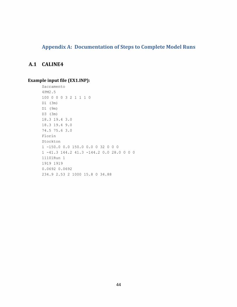
A.1 CALINE4

Example input file (EX1.INP): Sacramento 4PM2.5 100 0 0 0 3 2 1 1 1 0 D1 (3m) D1 (9m) D3 (3m) 18.3 19.4 3.0 18.3 19.4 9.0 74.5 75.6 3.0 Florin Stockton 1 -150.0 0.0 150.0 0.0 0 32 0 0 0 1 -41.3 144.2 41.3 -144.2 0.0 28.0 0 0 0 11101Run 1 1919 1919 0.0692 0.0692 234.9 2.53 2 1000 15.8 0 34.88

45

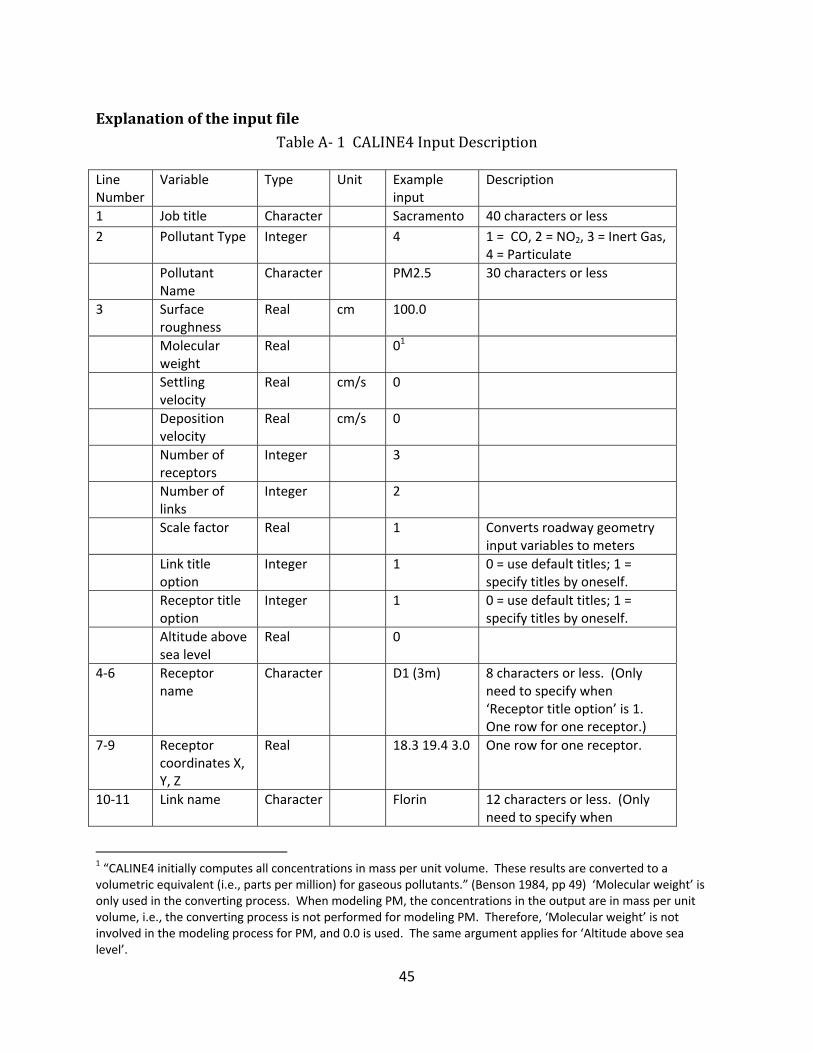
Explanation of the input file Table A‐ 1 CALINE4 Input Description Line Number

Variable Type Unit Example input

Description

1 Job title Character Sacramento 40 characters or less 2 Pollutant Type Integer 4 1 = CO, 2 = NO2, 3 = Inert Gas,

4 = Particulate Pollutant

Name Character PM2.5 30 characters or less

3 Surface roughness

Real cm 100.0

Molecular weight

Real 01

Settling velocity

Real cm/s 0

Deposition velocity

Real cm/s 0

Number of receptors

Integer 3

Number of links

Integer 2

Scale factor Real 1 Converts roadway geometry input variables to meters

Link title option

Integer 1 0 = use default titles; 1 = specify titles by oneself.

Receptor title option

Integer 1 0 = use default titles; 1 = specify titles by oneself.

Altitude above sea level

Real 0

4‐6 Receptor name

Character D1 (3m) 8 characters or less. (Only need to specify when ‘Receptor title option’ is 1. One row for one receptor.)

7‐9 Receptor coordinates X, Y, Z

Real 18.3 19.4 3.0 One row for one receptor.

10‐11 Link name Character Florin 12 characters or less. (Only need to specify when

1 “CALINE4 initially computes all concentrations in mass per unit volume. These results are converted to a volumetric equivalent (i.e., parts per million) for gaseous pollutants.” (Benson 1984, pp 49) ‘Molecular weight’ is only used in the converting process. When modeling PM, the concentrations in the output are in mass per unit volume, i.e., the converting process is not performed for modeling PM. Therefore, ‘Molecular weight’ is not involved in the modeling process for PM, and 0.0 is used. The same argument applies for ‘Altitude above sea level’.

46

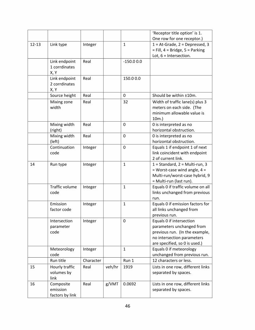
‘Receptor title option’ is 1. One row for one receptor.)

12‐13 Link type Integer 1 1 = At‐Grade, 2 = Depressed, 3 = Fill, 4 = Bridge, 5 = Parking Lot, 6 = Intersection.

Link endpoint 1 corrdinates X, Y

Real ‐150.0 0.0

Link endpoint 2 corrdinates X, Y

Real 150.0 0.0

Source height Real 0 Should be within ±10m. Mixing zone

width Real 32 Width of traffic lane(s) plus 3

meters on each side. (The minimum allowable value is 10m.)

Mixing width (right)

Real 0 0 is interpreted as no horizontal obstruction.

Mixing width (left)

Real 0 0 is interpreted as no horizontal obstruction.

Continuation code

Integer 0 Equals 1 if endpoint 1 of next link coincident with endpoint 2 of current link.

14 Run type Integer 1 1 = Standard, 2 = Multi‐run, 3 = Worst‐case wind angle, 4 = Multi‐run/worst‐case hybrid, 9 = Multi‐run (last run).

Traffic volume code

Integer 1 Equals 0 if traffic volume on all links unchanged from previous run.

Emission factor code

Integer 1 Equals 0 if emission factors for all links unchanged from previous run.

Intersection parameter code

Integer 0 Equals 0 if intersection parameters unchanged from previous run. (In the example, no intersection parameters are specified, so 0 is used.)

Meteorology code

Integer 1 Equals 0 if meteorology unchanged from previous run.

Run title Character Run 1 12 characters or less. 15 Hourly traffic

volumes by link

Real veh/hr 1919 Lists in one row, different links separated by spaces.

16 Composite emission factors by link

Real g/VMT 0.0692 Lists in one row, different links separated by spaces.

47

17 Wind direction Real degree 234.9 The direction the wind is blowing from, measured clockwise in degrees from the north. (This parameter is not used in calculation if “Worst‐Case” is selected.)

Wind speed Real m/s 2.53 Atmospheric

stability class Integer 2 Values 1 through 7 correspond

to the standard definitions for stability class A through G.

Mixing height Real m 1000 “Mixing height algorithm is primarily meant for study of special case nocturnal inversion, and may be bypass by assigning a value of 1000 meters or greater.” (Benson, 1984)(pp.100)

Wind direction standard deviation

Real degree 15.8

Ambient concentration

Real ppm 0 “The program automatically sums the contributions from each link to each receptor. After this has been completed for all receptors, an ambient value is added.” (Benson, 1984) (pp.32) Therefore, the ambient concentration is not involved in the calculation of increment.

Temperature Real °C 34.88 Source: The description of input variables uses information from the technical report documentation of

CALINE4 (Benson, 1984).

To execute the program, at the DOS prompt, go the directory with the executable program

(caline4_50.exe) and the input file, type:

caline4_50 <input file name> output file name

For example: caline4_50 <EX1.INP> EX1.OUT

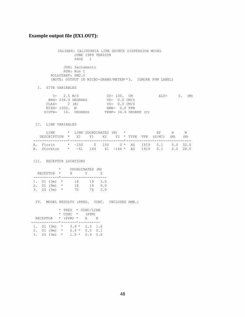
48

Example output file (EX1.OUT): CALINE4: CALIFORNIA LINE SOURCE DISPERSION MODEL JUNE 1989 VERSION PAGE 1 JOB: Sacramento RUN: Run 1 POLLUTANT: PM2.5 (NOTE: OUTPUT IN MICRO-GRAMS/METER**3. IGNORE PPM LABEL) I. SITE VARIABLES U= 2.5 M/S Z0= 100. CM ALT= 0. (M) BRG= 234.9 DEGREES VD= 0.0 CM/S CLAS= 2 (B) VS= 0.0 CM/S MIXH= 1000. M AMB= 0.0 PPM SIGTH= 16. DEGREES TEMP= 34.9 DEGREE (C) II. LINK VARIABLES LINK * LINK COORDINATES (M) * EF H W DESCRIPTION * X1 Y1 X2 Y2 * TYPE VPH (G/MI) (M) (M) ----------------*-------------------------*------------------------------ A. Florin * -150 0 150 0 * AG 1919 0.1 0.0 32.0 B. Stockton * -41 144 41 -144 * AG 1919 0.1 0.0 28.0 III. RECEPTOR LOCATIONS * COORDINATES (M) RECEPTOR * X Y Z ------------*--------------------- 1. D1 (3m) * 18 19 3.0 2. D1 (9m) * 18 19 9.0 3. D3 (3m) * 75 76 3.0 IV. MODEL RESULTS (PRED. CONC. INCLUDES AMB.) * PRED * CONC/LINK * CONC * (PPM) RECEPTOR * (PPM) * A B -------------*-------*---------- 1. D1 (3m) * 3.9 * 2.3 1.6 2. D1 (9m) * 0.4 * 0.3 0.1 3. D3 (3m) * 1.5 * 0.9 0.6

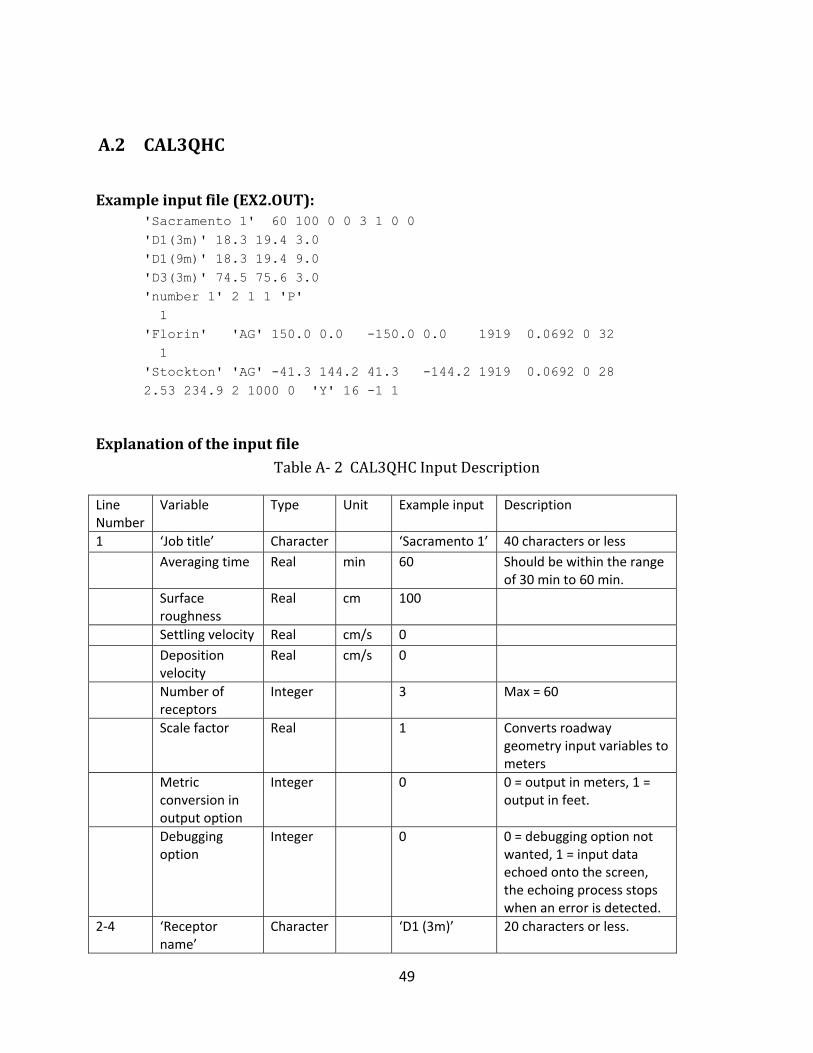
49

A.2 CAL3QHC

Example input file (EX2.OUT): 'Sacramento 1' 60 100 0 0 3 1 0 0 'D1(3m)' 18.3 19.4 3.0 'D1(9m)' 18.3 19.4 9.0 'D3(3m)' 74.5 75.6 3.0 'number 1' 2 1 1 'P' 1 'Florin' 'AG' 150.0 0.0 -150.0 0.0 1919 0.0692 0 32 1 'Stockton' 'AG' -41.3 144.2 41.3 -144.2 1919 0.0692 0 28 2.53 234.9 2 1000 0 'Y' 16 -1 1

Explanation of the input file Table A‐ 2 CAL3QHC Input Description Line Number

Variable Type Unit Example input Description

1 ‘Job title’ Character ‘Sacramento 1’ 40 characters or less Averaging time Real min 60 Should be within the range

of 30 min to 60 min. Surface

roughness Real cm 100

Settling velocity Real cm/s 0 Deposition

velocity Real cm/s 0

Number of receptors

Integer 3 Max = 60

Scale factor Real 1 Converts roadway geometry input variables to meters

Metric conversion in output option

Integer 0 0 = output in meters, 1 = output in feet.

Debugging option

Integer 0 0 = debugging option not wanted, 1 = input data echoed onto the screen, the echoing process stops when an error is detected.

2‐4 ‘Receptor name’

Character ‘D1 (3m)’ 20 characters or less.

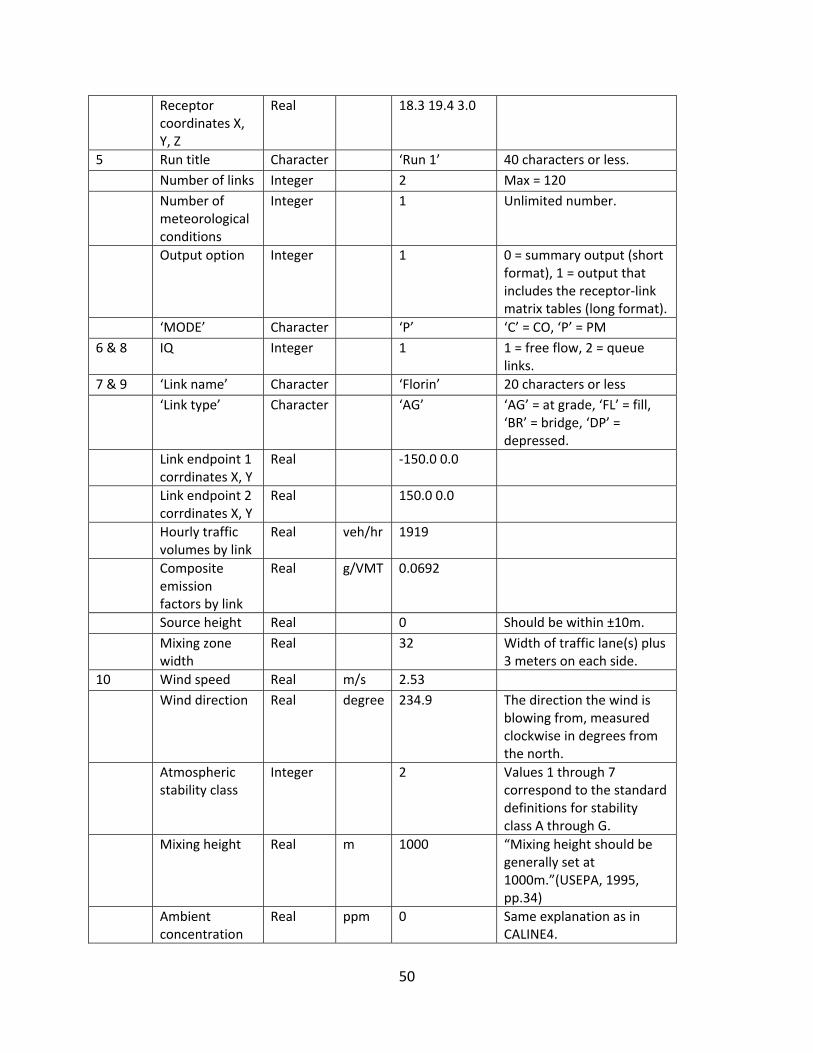
50

Receptor coordinates X, Y, Z

Real 18.3 19.4 3.0

5 Run title Character ‘Run 1’ 40 characters or less. Number of links Integer 2 Max = 120 Number of

meteorological conditions

Integer 1 Unlimited number.

Output option Integer 1 0 = summary output (short format), 1 = output that includes the receptor‐link matrix tables (long format).

‘MODE’ Character ‘P’ ‘C’ = CO, ‘P’ = PM 6 & 8 IQ Integer 1 1 = free flow, 2 = queue

links. 7 & 9 ‘Link name’ Character ‘Florin’ 20 characters or less ‘Link type’ Character ‘AG’ ‘AG’ = at grade, ‘FL’ = fill,

‘BR’ = bridge, ‘DP’ = depressed.

Link endpoint 1 corrdinates X, Y

Real ‐150.0 0.0

Link endpoint 2 corrdinates X, Y

Real 150.0 0.0

Hourly traffic volumes by link

Real veh/hr 1919

Composite emission factors by link

Real g/VMT 0.0692

Source height Real 0 Should be within ±10m. Mixing zone

width Real 32 Width of traffic lane(s) plus

3 meters on each side. 10 Wind speed Real m/s 2.53 Wind direction Real degree 234.9 The direction the wind is

blowing from, measured clockwise in degrees from the north.

Atmospheric stability class

Integer 2 Values 1 through 7 correspond to the standard definitions for stability class A through G.

Mixing height Real m 1000 “Mixing height should be generally set at 1000m.”(USEPA, 1995, pp.34)

Ambient concentration

Real ppm 0 Same explanation as in CALINE4.

51

‘Wind direction variation’

Character ‘Y’ ‘Y’ = allow wind direction to vary, ‘N’ = use only the specified wind direction.

Wind direction increment angle

Integer 16

First increment multiplier

Integer ‐1

Last increment multiplier

Integer 1

These three variables are not used in the case that ‘N’ is specified for ‘Wind direction variation’; however, these three variables have to be specified in order for the program to run. If ‘Y’ is specified for ‘Wind direction variation’, concentration under wind direction from first increment to last increment will be displayed in the output.

Source: The description of input variables uses information from the User’s Guide to CAL3QHC (USEPA,

1995).

To execute the program, at the DOS prompt, go the directory with the executable program

(CAL3QHC.exe) and the input file, type:

CAL3QHC input file name output file name

For example: CAL3QHC EX2.INP EX2.OUT

Example output file (EX2.OUT):

CAL3QHC: LINE SOURCE DISPERSION MODEL - VERSION 2.0 Dated 95221 PAGE 1 JOB: Sacramento 1 RUN: Run 1 DATE : 6/23/ 8 TIME : 1:20:38 The MODE flag has been set to P for calculating PM averages. SITE & METEOROLOGICAL VARIABLES ------------------------------- VS = 0.0 CM/S VD = 0.0 CM/S Z0 = 100. CM U = 2.5 M/S CLAS = 2 (B) ATIM = 60. MINUTES MIXH = 1000.M AMB = 0.0 ug/m**3 LINK VARIABLES -------------- LINK DESCRIPTION * LINK COORDINATES (M) * LENGTH BRG TYPE VPH EF H W V/C QUEUE

52

* X1 Y1 X2 Y2 * (M) (DEG) (G/MI) (M) (M) (VEH) ------------------------*---------------------------------*---------------------------------------------------------- 1. Florin * 150.0 0.0 -150.0 0.0 * 300. 270. AG 1919. 0.1 0.0 32.0 2. Stockton * -41.3 144.2 41.3 -144.2 * 300. 164. AG 1919. 0.1 0.0 28.0 PAGE 2 JOB: Sacramento 1 RUN: Run 1 DATE : 6/23/ 8 TIME : 1:20:38 RECEPTOR LOCATIONS ------------------ * COORDINATES (M) * RECEPTOR * X Y Z * -------------------------*------------------------------------------* 1. D1(3m) * 18.3 19.4 3.0 * 2. D1(9m) * 18.3 19.4 9.0 * 3. D3(3m) * 74.5 75.6 3.0 * MODEL RESULTS ------------- REMARKS : In search of the angle corresponding to the maximum concentration, only the first angle, of the angles with same maximum concentrations, is indicated as maximum. WIND ANGLE RANGE: 219.-251. WIND * CONCENTRATION ANGLE * (ug/m**3) (DEGR) * REC1 REC2 REC3 ------------*-------------------------- 219. * 3. 1. 1. 235. * 3. 1. 1. 251. * 3. 1. 1. ------------*--------------------------- MAX * 3. 1. 1. DEGR. * 234 218 218 THE HIGHEST CONCENTRATION OF 3. ug/m**3 OCCURRED AT RECEPTOR REC1 . PAGE 3 JOB: Sacramento 1 RUN: Run 1 DATE : 6/23/ 8 TIME : 1:20:38 RECEPTOR - LINK MATRIX FOR THE ANGLE PRODUCING THE MAXIMUM CONCENTRATION FOR EACH RECEPTOR

53

* PM/LNK(ug/m**3) * ANGLE (DEGREES) * REC1 REC2 REC3 LINK # * 234 218 218 ------------*---------------------------- 1 * 1.4 0.4 0.5 2 * 1.3 0.4 0.4

We can get the predicted PM2.5 concentration in ‘PAGE 3’ of the output file.

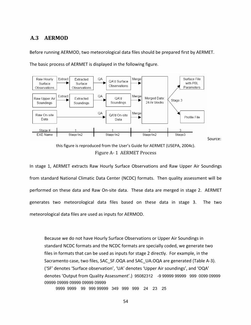
54

A.3 AERMOD

Before running AERMOD, two meteorological data files should be prepared first by AERMET.

The basic process of AERMET is displayed in the following figure.

Source:

this figure is reproduced from the User’s Guide for AERMET (USEPA, 2004c). Figure A‐ 1 AERMET Process

In stage 1, AERMET extracts Raw Hourly Surface Observations and Raw Upper Air Soundings

from standard National Climatic Data Center (NCDC) formats. Then quality assessment will be

performed on these data and Raw On‐site data. These data are merged in stage 2. AERMET

generates two meteorological data files based on these data in stage 3. The two

meteorological data files are used as inputs for AERMOD.

Because we do not have Hourly Surface Observations or Upper Air Soundings in

standard NCDC formats and the NCDC formats are specially coded, we generate two

files in formats that can be used as inputs for stage 2 directly. For example, in the

Sacramento case, two files, SAC_SF.OQA and SAC_UA.OQA are generated (Table A‐3).

(‘SF’ denotes ‘Surface observation’, ‘UA’ denotes ‘Upper Air soundings’, and ‘OQA’

denotes ‘Output from Quality Assessment’.) 95082312 -9 99999 99999 999 0099 09999 09999 09999 09999 09999 09999 9999 9999 99 999 99999 349 999 999 24 23 25

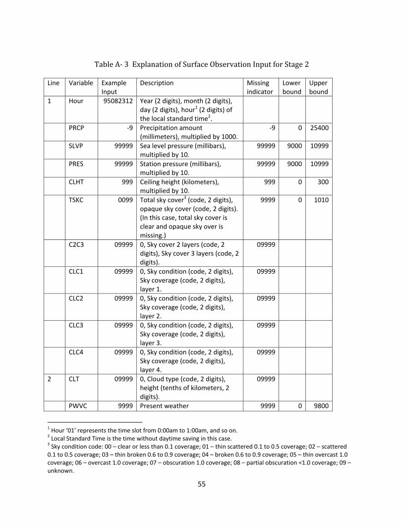
55

Table A‐ 3 Explanation of Surface Observation Input for Stage 2 Line Variable Example

Input Description Missing

indicator Lower bound

Upper bound

1 Hour 95082312 Year (2 digits), month (2 digits), day (2 digits), hour1 (2 digits) of the local standard time2.

PRCP ‐9 Precipitation amount (millimeters), multiplied by 1000.

‐9 0 25400

SLVP 99999 Sea level pressure (millibars), multiplied by 10.

99999 9000 10999

PRES 99999 Station pressure (millibars), multiplied by 10.

99999 9000 10999

CLHT 999 Ceiling height (kilometers), multiplied by 10.

999 0 300

TSKC 0099 Total sky cover3 (code, 2 digits), opaque sky cover (code, 2 digits). (In this case, total sky cover is clear and opaque sky over is missing.)

9999 0 1010

C2C3 09999 0, Sky cover 2 layers (code, 2 digits), Sky cover 3 layers (code, 2 digits).

09999

CLC1 09999 0, Sky condition (code, 2 digits), Sky coverage (code, 2 digits), layer 1.

09999

CLC2 09999 0, Sky condition (code, 2 digits), Sky coverage (code, 2 digits), layer 2.

09999

CLC3 09999 0, Sky condition (code, 2 digits), Sky coverage (code, 2 digits), layer 3.

09999

CLC4 09999 0, Sky condition (code, 2 digits), Sky coverage (code, 2 digits), layer 4.

09999

2 CLT 09999 0, Cloud type (code, 2 digits), height (tenths of kilometers, 2 digits).

09999

PWVC 9999 Present weather 9999 0 9800

1 Hour ‘01’ represents the time slot from 0:00am to 1:00am, and so on. 2 Local Standard Time is the time without daytime saving in this case. 3 Sky condition code: 00 – clear or less than 0.1 coverage; 01 – thin scattered 0.1 to 0.5 coverage; 02 – scattered 0.1 to 0.5 coverage; 03 – thin broken 0.6 to 0.9 coverage; 04 – broken 0.6 to 0.9 coverage; 05 – thin overcast 1.0 coverage; 06 – overcast 1.0 coverage; 07 – obscuration 1.0 coverage; 08 – partial obscuration <1.0 coverage; 09 – unknown.

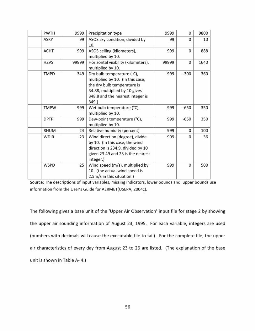
56

PWTH 9999 Precipitation type 9999 0 9800

ASKY 99 ASOS sky condition, divided by 10.

99 0 10

ACHT 999 ASOS ceiling (kilometers), multiplied by 10.

999 0 888

HZVS 99999 Horizontal visibility (kilometers), multiplied by 10.

99999 0 1640

TMPD 349 Dry bulb temperature (oC), multiplied by 10. (In this case, the dry bulb temperature is 34.88, multiplied by 10 gives 348.8 and the nearest integer is 349.)

999 ‐300 360

TMPW 999 Wet bulb temperature (oC), multiplied by 10.

999 ‐650 350

DPTP 999 Dew‐point temperature (oC), multiplied by 10.

999 ‐650 350

RHUM 24 Relative humidity (percent) 999 0 100

WDIR 23 Wind direction (degree), divide by 10. (In this case, the wind direction is 234.9, divided by 10 given 23.49 and 23 is the nearest integer.)

999 0 36

WSPD 25 Wind speed (m/s), multiplied by 10. (the actual wind speed is 2.5m/s in this situation.)

999 0 500

Source: The descriptions of input variables, missing indicators, lower bounds and upper bounds use

information from the User’s Guide for AERMET(USEPA, 2004c).

The following gives a base unit of the ‘Upper Air Observation’ input file for stage 2 by showing

the upper air sounding information of August 23, 1995. For each variable, integers are used

(numbers with decimals will cause the executable file to fail). For the complete file, the upper

air characteristics of every day from August 23 to 26 are listed. (The explanation of the base

unit is shown in Table A‐ 4.)

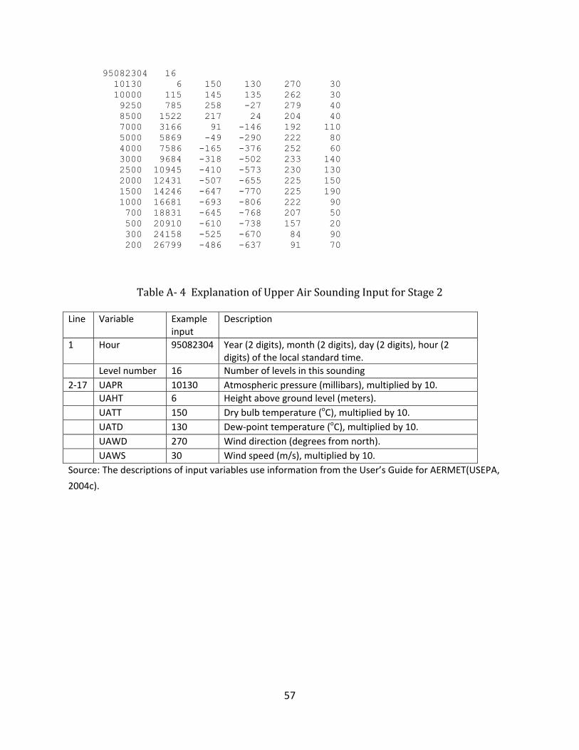
57

95082304 16 10130 6 150 130 270 30 10000 115 145 135 262 30 9250 785 258 -27 279 40 8500 1522 217 24 204 40 7000 3166 91 -146 192 110 5000 5869 -49 -290 222 80 4000 7586 -165 -376 252 60 3000 9684 -318 -502 233 140 2500 10945 -410 -573 230 130 2000 12431 -507 -655 225 150 1500 14246 -647 -770 225 190 1000 16681 -693 -806 222 90 700 18831 -645 -768 207 50 500 20910 -610 -738 157 20 300 24158 -525 -670 84 90 200 26799 -486 -637 91 70

Table A‐ 4 Explanation of Upper Air Sounding Input for Stage 2 Line Variable Example

input Description

1 Hour 95082304 Year (2 digits), month (2 digits), day (2 digits), hour (2 digits) of the local standard time.

Level number 16 Number of levels in this sounding 2‐17 UAPR 10130 Atmospheric pressure (millibars), multiplied by 10. UAHT 6 Height above ground level (meters). UATT 150 Dry bulb temperature (oC), multiplied by 10. UATD 130 Dew‐point temperature (oC), multiplied by 10. UAWD 270 Wind direction (degrees from north). UAWS 30 Wind speed (m/s), multiplied by 10. Source: The descriptions of input variables use information from the User’s Guide for AERMET(USEPA,

2004c).

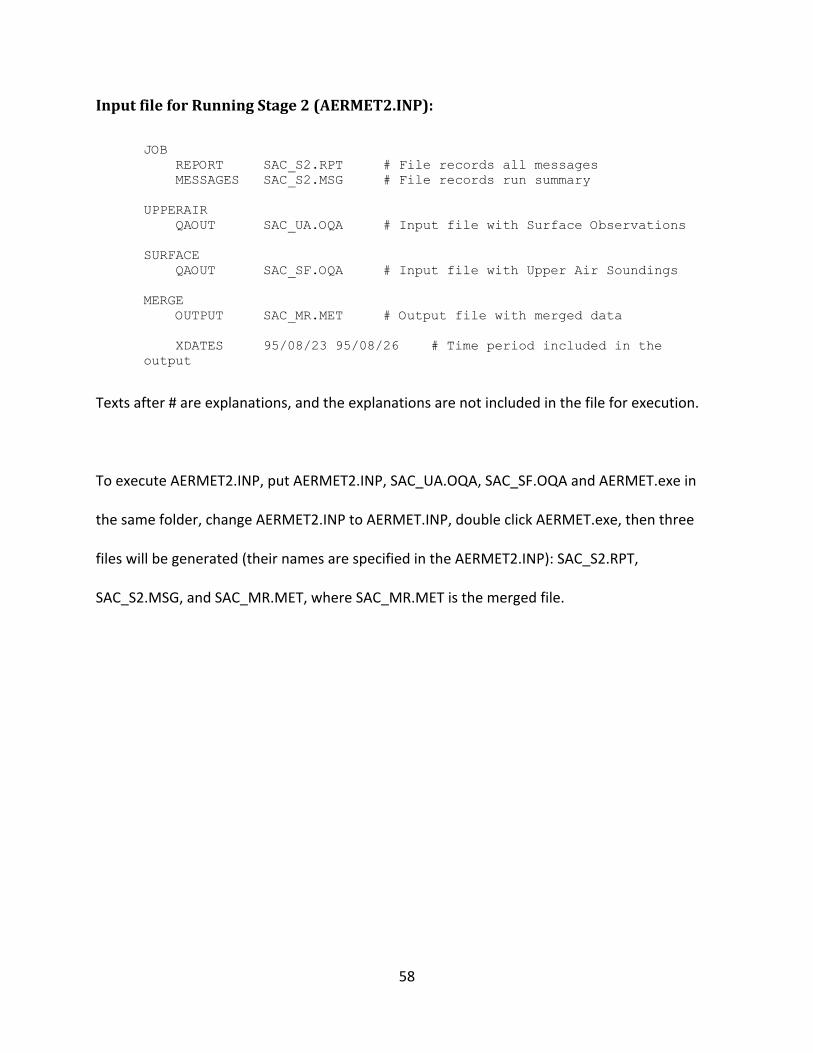
58

Input file for Running Stage 2 (AERMET2.INP):

JOB REPORT SAC_S2.RPT # File records all messages MESSAGES SAC_S2.MSG # File records run summary UPPERAIR QAOUT SAC_UA.OQA # Input file with Surface Observations SURFACE QAOUT SAC_SF.OQA # Input file with Upper Air Soundings MERGE OUTPUT SAC_MR.MET # Output file with merged data XDATES 95/08/23 95/08/26 # Time period included in the output

Texts after # are explanations, and the explanations are not included in the file for execution.

To execute AERMET2.INP, put AERMET2.INP, SAC_UA.OQA, SAC_SF.OQA and AERMET.exe in

the same folder, change AERMET2.INP to AERMET.INP, double click AERMET.exe, then three

files will be generated (their names are specified in the AERMET2.INP): SAC_S2.RPT,

SAC_S2.MSG, and SAC_MR.MET, where SAC_MR.MET is the merged file.

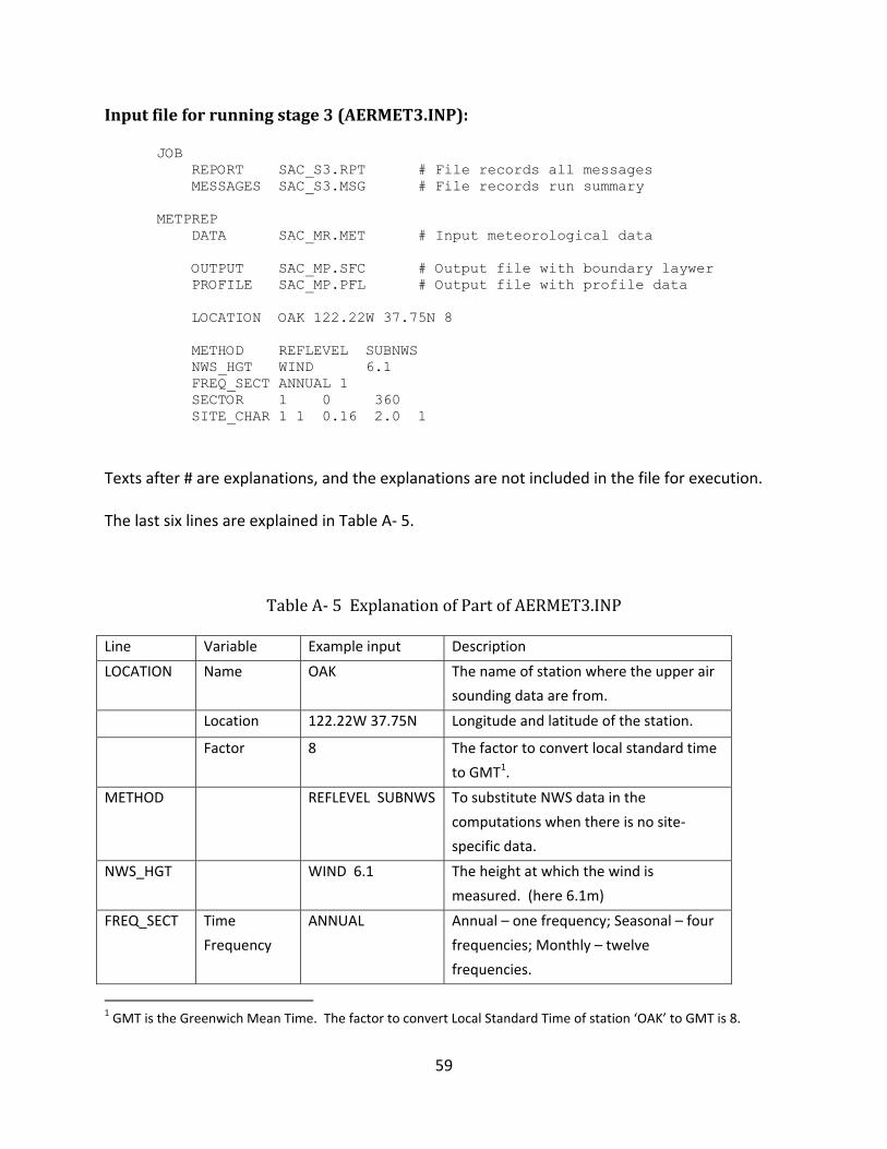
59

Input file for running stage 3 (AERMET3.INP):

JOB REPORT SAC_S3.RPT # File records all messages MESSAGES SAC_S3.MSG # File records run summary METPREP DATA SAC_MR.MET # Input meteorological data OUTPUT SAC_MP.SFC # Output file with boundary laywer PROFILE SAC_MP.PFL # Output file with profile data LOCATION OAK 122.22W 37.75N 8 METHOD REFLEVEL SUBNWS NWS_HGT WIND 6.1 FREQ_SECT ANNUAL 1 SECTOR 1 0 360 SITE_CHAR 1 1 0.16 2.0 1

Texts after # are explanations, and the explanations are not included in the file for execution.

The last six lines are explained in Table A‐ 5.

Table A‐ 5 Explanation of Part of AERMET3.INP Line Variable Example input Description

LOCATION Name OAK The name of station where the upper air

sounding data are from.

Location 122.22W 37.75N Longitude and latitude of the station.

Factor 8 The factor to convert local standard time

to GMT1.

METHOD REFLEVEL SUBNWS To substitute NWS data in the

computations when there is no site‐

specific data.

NWS_HGT WIND 6.1 The height at which the wind is

measured. (here 6.1m)

FREQ_SECT Time

Frequency ANNUAL Annual – one frequency; Seasonal – four

frequencies; Monthly – twelve

frequencies.

1 GMT is the Greenwich Mean Time. The factor to convert Local Standard Time of station ‘OAK’ to GMT is 8.

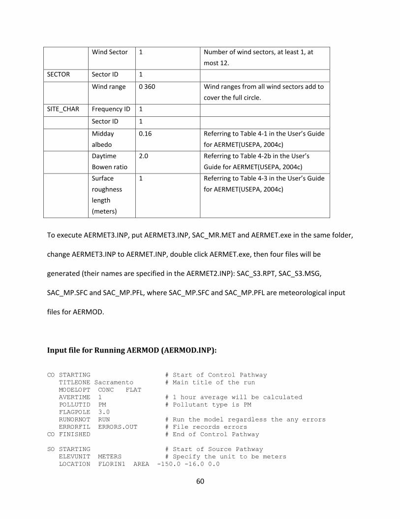
60

Wind Sector 1 Number of wind sectors, at least 1, at

most 12.

SECTOR Sector ID 1

Wind range 0 360 Wind ranges from all wind sectors add to

cover the full circle.

SITE_CHAR Frequency ID 1

Sector ID 1

Midday

albedo 0.16 Referring to Table 4‐1 in the User’s Guide

for AERMET(USEPA, 2004c)

Daytime

Bowen ratio 2.0 Referring to Table 4‐2b in the User’s

Guide for AERMET(USEPA, 2004c)

Surface

roughness

length

(meters)

1 Referring to Table 4‐3 in the User’s Guide

for AERMET(USEPA, 2004c)

To execute AERMET3.INP, put AERMET3.INP, SAC_MR.MET and AERMET.exe in the same folder,

change AERMET3.INP to AERMET.INP, double click AERMET.exe, then four files will be

generated (their names are specified in the AERMET2.INP): SAC_S3.RPT, SAC_S3.MSG,

SAC_MP.SFC and SAC_MP.PFL, where SAC_MP.SFC and SAC_MP.PFL are meteorological input

files for AERMOD.

Input file for Running AERMOD (AERMOD.INP):

CO STARTING # Start of Control Pathway TITLEONE Sacramento # Main title of the run MODELOPT CONC FLAT AVERTIME 1 # 1 hour average will be calculated POLLUTID PM # Pollutant type is PM FLAGPOLE 3.0 RUNORNOT RUN # Run the model regardless the any errors ERRORFIL ERRORS.OUT # File records errors CO FINISHED # End of Control Pathway SO STARTING # Start of Source Pathway ELEVUNIT METERS # Specify the unit to be meters LOCATION FLORIN1 AREA -150.0 -16.0 0.0

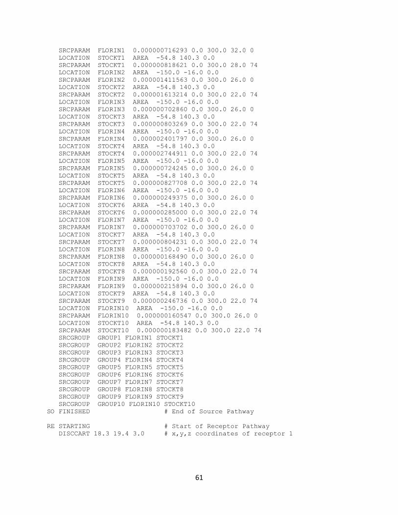
61

SRCPARAM FLORIN1 0.000000716293 0.0 300.0 32.0 0 LOCATION STOCKT1 AREA -54.8 140.3 0.0 SRCPARAM STOCKT1 0.000000818621 0.0 300.0 28.0 74 LOCATION FLORIN2 AREA -150.0 -16.0 0.0 SRCPARAM FLORIN2 0.000001411563 0.0 300.0 26.0 0 LOCATION STOCKT2 AREA -54.8 140.3 0.0 SRCPARAM STOCKT2 0.000001613214 0.0 300.0 22.0 74 LOCATION FLORIN3 AREA -150.0 -16.0 0.0 SRCPARAM FLORIN3 0.000000702860 0.0 300.0 26.0 0 LOCATION STOCKT3 AREA -54.8 140.3 0.0 SRCPARAM STOCKT3 0.000000803269 0.0 300.0 22.0 74 LOCATION FLORIN4 AREA -150.0 -16.0 0.0 SRCPARAM FLORIN4 0.000002401797 0.0 300.0 26.0 0 LOCATION STOCKT4 AREA -54.8 140.3 0.0 SRCPARAM STOCKT4 0.000002744911 0.0 300.0 22.0 74 LOCATION FLORIN5 AREA -150.0 -16.0 0.0 SRCPARAM FLORIN5 0.000000724245 0.0 300.0 26.0 0 LOCATION STOCKT5 AREA -54.8 140.3 0.0 SRCPARAM STOCKT5 0.000000827708 0.0 300.0 22.0 74 LOCATION FLORIN6 AREA -150.0 -16.0 0.0 SRCPARAM FLORIN6 0.000000249375 0.0 300.0 26.0 0 LOCATION STOCKT6 AREA -54.8 140.3 0.0 SRCPARAM STOCKT6 0.000000285000 0.0 300.0 22.0 74 LOCATION FLORIN7 AREA -150.0 -16.0 0.0 SRCPARAM FLORIN7 0.000000703702 0.0 300.0 26.0 0 LOCATION STOCKT7 AREA -54.8 140.3 0.0 SRCPARAM STOCKT7 0.000000804231 0.0 300.0 22.0 74 LOCATION FLORIN8 AREA -150.0 -16.0 0.0 SRCPARAM FLORIN8 0.000000168490 0.0 300.0 26.0 0 LOCATION STOCKT8 AREA -54.8 140.3 0.0 SRCPARAM STOCKT8 0.000000192560 0.0 300.0 22.0 74 LOCATION FLORIN9 AREA -150.0 -16.0 0.0 SRCPARAM FLORIN9 0.000000215894 0.0 300.0 26.0 0 LOCATION STOCKT9 AREA -54.8 140.3 0.0 SRCPARAM STOCKT9 0.000000246736 0.0 300.0 22.0 74 LOCATION FLORIN10 AREA -150.0 -16.0 0.0 SRCPARAM FLORIN10 0.000000160547 0.0 300.0 26.0 0 LOCATION STOCKT10 AREA -54.8 140.3 0.0 SRCPARAM STOCKT10 0.000000183482 0.0 300.0 22.0 74 SRCGROUP GROUP1 FLORIN1 STOCKT1 SRCGROUP GROUP2 FLORIN2 STOCKT2 SRCGROUP GROUP3 FLORIN3 STOCKT3 SRCGROUP GROUP4 FLORIN4 STOCKT4 SRCGROUP GROUP5 FLORIN5 STOCKT5 SRCGROUP GROUP6 FLORIN6 STOCKT6 SRCGROUP GROUP7 FLORIN7 STOCKT7 SRCGROUP GROUP8 FLORIN8 STOCKT8 SRCGROUP GROUP9 FLORIN9 STOCKT9 SRCGROUP GROUP10 FLORIN10 STOCKT10 SO FINISHED # End of Source Pathway RE STARTING # Start of Receptor Pathway DISCCART 18.3 19.4 3.0 # x,y,z coordinates of receptor 1

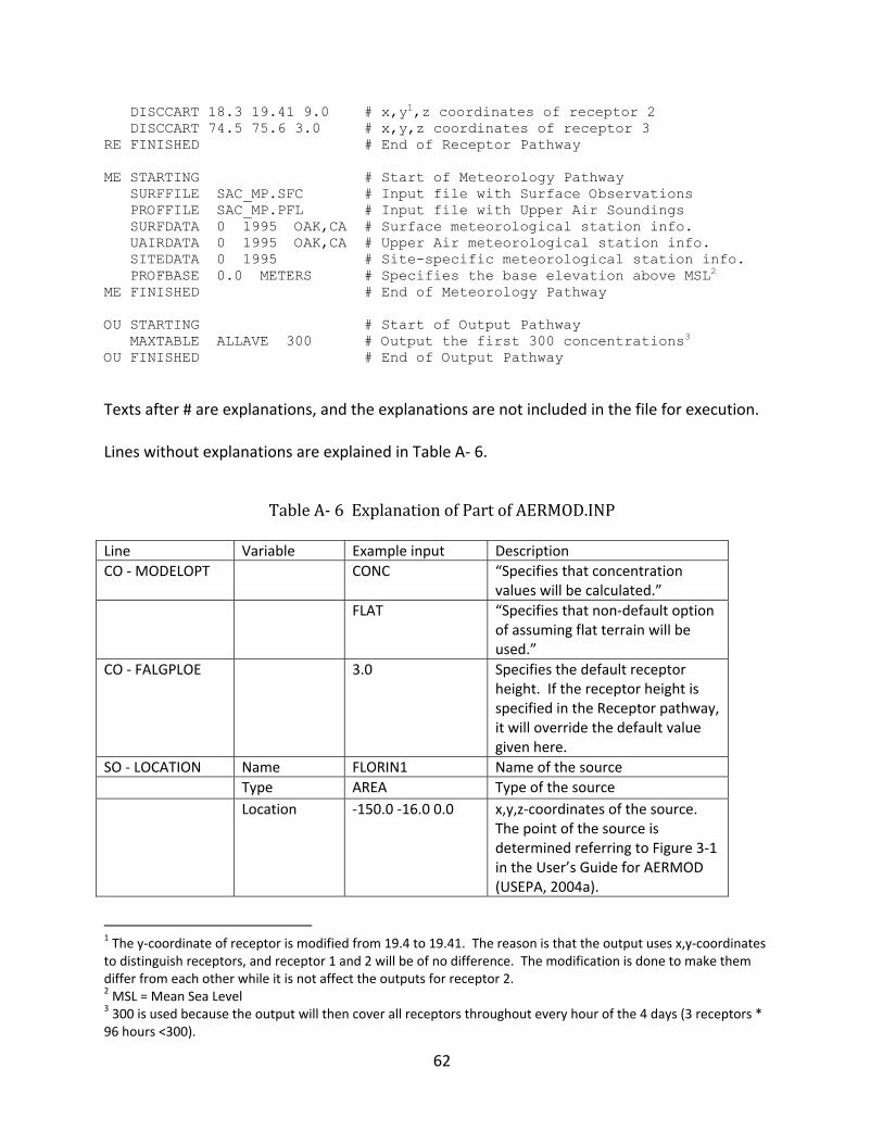
62

DISCCART 18.3 19.41 9.0 # x,y1,z coordinates of receptor 2 DISCCART 74.5 75.6 3.0 # x,y,z coordinates of receptor 3 RE FINISHED # End of Receptor Pathway ME STARTING # Start of Meteorology Pathway SURFFILE SAC_MP.SFC # Input file with Surface Observations PROFFILE SAC_MP.PFL # Input file with Upper Air Soundings SURFDATA 0 1995 OAK,CA # Surface meteorological station info. UAIRDATA 0 1995 OAK,CA # Upper Air meteorological station info. SITEDATA 0 1995 # Site-specific meteorological station info. PROFBASE 0.0 METERS # Specifies the base elevation above MSL2 ME FINISHED # End of Meteorology Pathway OU STARTING # Start of Output Pathway MAXTABLE ALLAVE 300 # Output the first 300 concentrations3 OU FINISHED # End of Output Pathway Texts after # are explanations, and the explanations are not included in the file for execution.

Lines without explanations are explained in Table A‐ 6.

Table A‐ 6 Explanation of Part of AERMOD.INP Line Variable Example input Description CO ‐ MODELOPT CONC “Specifies that concentration

values will be calculated.” FLAT “Specifies that non‐default option

of assuming flat terrain will be used.”

CO ‐ FALGPLOE 3.0 Specifies the default receptor height. If the receptor height is specified in the Receptor pathway, it will override the default value given here.

SO ‐ LOCATION Name FLORIN1 Name of the source Type AREA Type of the source Location ‐150.0 ‐16.0 0.0 x,y,z‐coordinates of the source.

The point of the source is determined referring to Figure 3‐1 in the User’s Guide for AERMOD (USEPA, 2004a).

1 The y‐coordinate of receptor is modified from 19.4 to 19.41. The reason is that the output uses x,y‐coordinates to distinguish receptors, and receptor 1 and 2 will be of no difference. The modification is done to make them differ from each other while it is not affect the outputs for receptor 2. 2 MSL = Mean Sea Level 3 300 is used because the output will then cover all receptors throughout every hour of the 4 days (3 receptors * 96 hours <300).

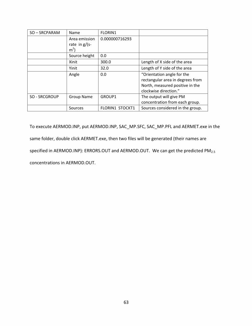
63

SO – SRCPARAM Name FLORIN1 Area emission

rate in g/(s‐ m2)

0.000000716293

Source height 0.0 Xinit 300.0 Length of X side of the area Yinit 32.0 Length of Y side of the area Angle 0.0 “Orientation angle for the

rectangular area in degrees from North, measured positive in the clockwise direction.”

SO ‐ SRCGROUP Group Name GROUP1 The output will give PM concentration from each group.

Sources FLORIN1 STOCKT1 Sources considered in the group.

To execute AERMOD.INP, put AERMOD.INP, SAC_MP.SFC, SAC_MP.PFL and AERMET.exe in the

same folder, double click AERMET.exe, then two files will be generated (their names are

specified in AERMOD.INP): ERRORS.OUT and AERMOD.OUT. We can get the predicted PM2.5

concentrations in AERMOD.OUT.

64

Appendix B: Abbreviations

AERMET = AERmod’s METeorological data preprocessor (a meteorological data preprocessor

for AERMOD)

AERMOD = American Meteorological Society (Ams) and U.S. Environmental Protection Agency

(Epa) Regulatory MODel

CAL3QHC = CALINE3 with Queuing and Hot‐spot Calculations

CALINE3 = California LINE source dispersion model version 3

CALINE4 = California LINE source dispersion model version 4

CBL = Convective Boundary Layer

EPA = Environmental Protection Agency

GMT = Greenwich Mean Time

MSL = Mean Sea Level

PM = Particulate Matter

PM2.5 = Particulate Matter less than 2.5 µm

PM10 = Particulate Matter less than 10 µm

PBL = Planetary Boundary Layer

SBL = Stable Boundary Layer