Modeling the Arsenic Biosensor System - 2006.igem.org

Modeling the Arsenic Biosensor System

Yizhi Cai‡, Bryony Davidson§, Hongwu Ma‡, Chris French¶

From the ‡School of Informatics, §School of Engineering, ¶School of Biology

University of Edinburgh

Abstract This paper reports the modeling

progress of an arsenic biosensor system, which is

the iGEM project accomplished in the University

of Edinburgh 2006. The arsenic biosensor system

sought to address the fatal water pollution

problem occurring in many poor countries/areas

like Bangladesh by producing a calibratable pH

changes in response to a range of arsenic

concentrations. A computational model which

contains 3 operons, 19 reactions and 17 species

has been constructed to shed light on the wet-lab

experimental design. By analyzing the sensitivity

of each parameter/species, we identified their

relative importance in the system which gives the

theoretical guide when measuring the variable in

wet-lab. The next step research is to refine the

model by comparing it with the biological output.

Key words Modeling, Arsenic Biosensor, Edinburgh iGEM 2006

Methodology

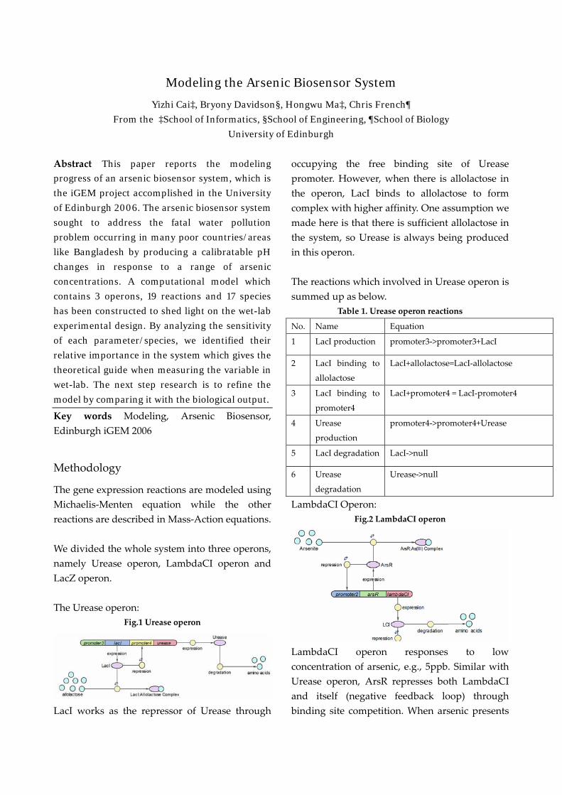
The gene expression reactions are modeled using Michaelis‐Menten equation while the other reactions are described in Mass‐Action equations. We divided the whole system into three operons, namely Urease operon, LambdaCI operon and LacZ operon. The Urease operon:

Fig.1 Urease operon

LacI works as the repressor of Urease through

occupying the free binding site of Urease promoter. However, when there is allolactose in the operon, LacI binds to allolactose to form complex with higher affinity. One assumption we made here is that there is sufficient allolactose in the system, so Urease is always being produced in this operon. The reactions which involved in Urease operon is summed up as below.

Table 1. Urease operon reactions

No. Name Equation

1 LacI production promoter3‐>promoter3+LacI

2 LacI binding to

allolactose

LacI+allolactose=LacI‐allolactose

3 LacI binding to

promoter4

LacI+promoter4 = LacI‐promoter4

4 Urease

production

promoter4‐>promoter4+Urease

5 LacI degradation LacI‐>null

6 Urease

degradation

Urease‐>null

LambdaCI Operon: Fig.2 LambdaCI operon

LambdaCI operon responses to low concentration of arsenic, e.g., 5ppb. Similar with Urease operon, ArsR represses both LambdaCI and itself (negative feedback loop) through binding site competition. When arsenic presents

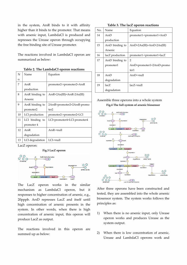
in the system, ArsR binds to it with affinity higher than it binds to the promoter. That means with arsenic input, LambdaCI is produced and represses the Urease operon through occupying the free binding site of Urease promoter. The reactions involved in LambdaCI operon are summarized as below:

Table 2. The LambdaCI operon reactions N

o.

Name Equation

7 ArsR

production

promoter2‐>promoter2+ArsR

8 ArsR binding to

Arsenic

ArsR+2As(III)=ArsR‐2As(III)

9 ArsR binding to

promoter2

2ArsR+promoter2=2ArsR‐promo

ter2

10 LCI production promoter2‐>promoter2+LCI

11 LCI binding to

promoter 4

LCI+promoter4=LCI‐promoter4

12 ArsR

degradation

ArsR‐>null

13 LCI degradation LCI‐>null

LacZ operon: Fig.3 LacZ operon

The LacZ operon works in the similar mechanism as LambdaCI operon, but it responses to higher concentration of arsenic, e.g., 20pppb. ArsD represses LacZ and itself until high concentration of arsenic presents in the system. In other words, when there is high concentration of arsenic input, this operon will produce LacZ as output. The reactions involved in this operon are summed up as below:

Table 3. The lacZ operon reactions No. Name Equation

14 ArsD

production

promoter1‐>promoter1+ArsD

15 ArsD binding to

Arsenic

ArsD+2As(III)=ArsD‐2As(III)

16 lacZ production promoter1‐>promoter1+lacZ

17 ArsD binding to

promoter1

2

ArsD+promoter1=2ArsD‐promo

ter1

18 ArsD

degradation

ArsD‐>null

19 lacZ

degradation

lacZ‐>null

Assemble three operons into a whole system

Fig.4 The full system of arsenic biosensor

After three operons have been constructed and tested, they are assembled into the whole arsenic biosensor system. The system works follows the principles as: 1) When there is no arsenic input, only Urease

operon works and produces Urease as the system output.

2) When there is low concentration of arsenic,

Urease and LambdaCI operons work and

produce Urease and LambdaCI. Because LambdaCI represses the production of Urease, the concentration of Urease is lower than no arsenic condition.

3) When the concentration of arsenic rises to

high level, all three operons work together. LacZ is produced together with Urease.

The complete reaction set is given with the initial condition bellow: Table 4. Reaction Set1

No. Name Equation Rate Law Parameters

1 LacI production promoter3‐>promoter3+LacI Michaelis‐Menten V12m=0.5, K12m=40

2 LacI binding to

allolactose

LacI+allolactose=LacI‐allolactose Mass Action K9=10000, K‐9=0.1

3 LacI binding to

promoter4

LacI+promoter4 = LacI‐promoter4 Mass Action K10=1000, K‐10=0.5

4 Urease production promoter4‐>promoter4+Urease Michaelis‐Menten V19m=10, K19m=40

5 LacI degradation LacI‐>null Mass Action K11=0.1

6 Urease degradation Urease‐>null Mass Action K18=0.1

7 ArsR production promoter2‐>promoter2+ArsR Michaelis‐Menten V8m=10, K8m=25

8 ArsR binding to

Arsenic (III)

ArsR+2As(III)=ArsR‐2As(III) Mass Action K5=1000, K‐5=0.65

9 ArsR binding to

promoter2

2ArsR+promoter2=2ArsR‐promoter2 Mass Action K6=10000, K‐6=0.65

10 LCI production promoter2‐>promoter2+LCI Michaelis‐Menten V17m=10, K17m=25

11 LCI binding to

promoter 4

LCI+promoter4=LCI‐promoter4 Mass Action K15=10000, K‐15=0.5

12 ArsR degradation ArsR‐>null Mass Action K7=0.05

13 LCI degradation LCI‐>null Mass Action K16=0.1

14 ArsD production promoter1‐>promoter1+ArsD Michaelis‐Menten V4m=0.5, K4m=75

15 ArsD binding to

Arsenic (III)

ArsD+2As(III)=ArsD‐2As(III) Mass Action K1=1000 K‐1=0.65

16 lacZ production promoter1‐>promoter1+lacZ Michaelis‐Menten V14m=25, K14m=10

17 ArsD binding to

promoter1

2 ArsD+promoter1=2ArsD‐promoter1 Mass Action K2=10000, K‐2=0.65

18 ArsD degradation ArsD‐>null Mass Action K3=0.05

19 lacZ degradation lacZ‐>null Mass Action K13=0.1

Table 5. Initial Concentration

No. Species Initial Concentration (nMol)

ArsD 25

As(III) 40

2ArsD‐promoter1 25

promoter1 5

ArsR 25

2ArsR‐promoter2 25

1 The units for first, second and third order rate constants are expressed in units of second‐1, nMol‐1×second‐1 and nMol‐2×second‐1 respectively.

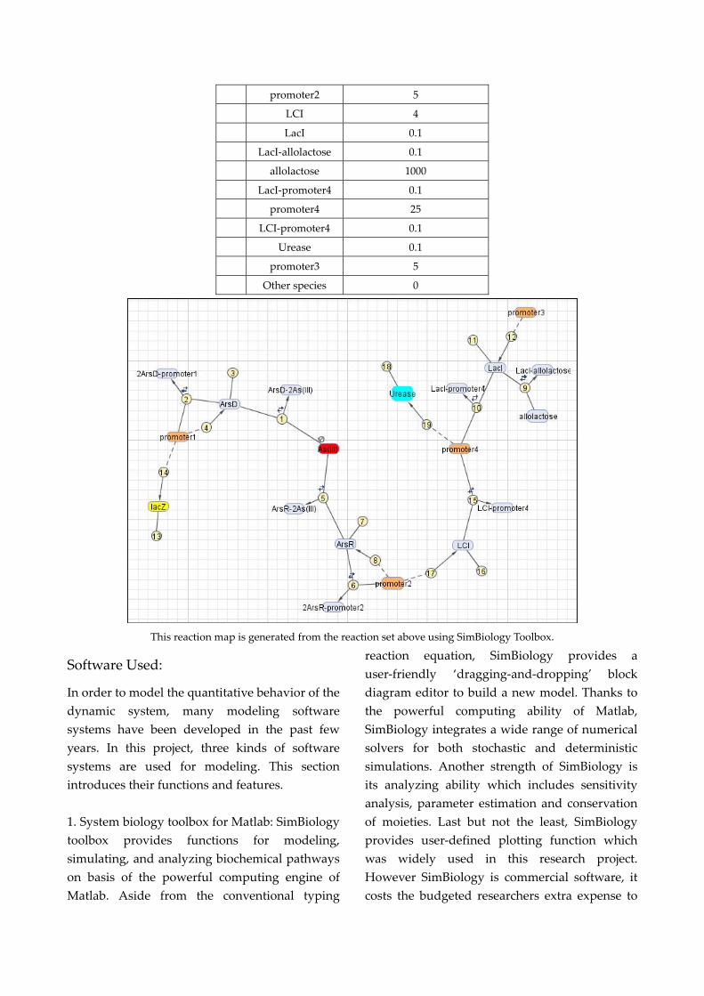
promoter2 5

LCI 4

LacI 0.1

LacI‐allolactose 0.1

allolactose 1000

LacI‐promoter4 0.1

promoter4 25

LCI‐promoter4 0.1

Urease 0.1

promoter3 5

Other species 0

This reaction map is generated from the reaction set above using SimBiology Toolbox.

Software Used:

In order to model the quantitative behavior of the dynamic system, many modeling software systems have been developed in the past few years. In this project, three kinds of software systems are used for modeling. This section introduces their functions and features. 1. System biology toolbox for Matlab: SimBiology toolbox provides functions for modeling, simulating, and analyzing biochemical pathways on basis of the powerful computing engine of Matlab. Aside from the conventional typing

reaction equation, SimBiology provides a user‐friendly ‘dragging‐and‐dropping’ block diagram editor to build a new model. Thanks to the powerful computing ability of Matlab, SimBiology integrates a wide range of numerical solvers for both stochastic and deterministic simulations. Another strength of SimBiology is its analyzing ability which includes sensitivity analysis, parameter estimation and conservation of moieties. Last but not the least, SimBiology provides user‐defined plotting function which was widely used in this research project. However SimBiology is commercial software, it costs the budgeted researchers extra expense to

purchase the license for this toolbox. Also, there is no GUI for sensitivity analysis and parameters scan functions, so users should obtain the skill of programming with Matlab. 2. BIOCHAM: BIOCHAM stands for biochemical abstract machine which is a formal modeling environment for system biology. Because of its rule‐based language and temporal logic based language, BIOCHAM can offer an automatically reasoning tool for querying the temporal properties of the system under all its possible behaviors. It is very useful for constructing models especially when numerical data is unavailable. BIOCHAM also provides a state‐of‐the‐art symbolic model checker for handling the complexity of large highly non‐deterministic models. Furthermore, it provides simulation results via its graphical interface. One disadvantage of BIOCHAM is that because it is initially developed under UNIX, it uses command line rather than GUI to build new models, requiring users to write scripts by hand. Another problem was that when transplanting the program from UNIX to Windows, the model checker of NuSMV does not work well. So this project used BIOCHAM in Fedora 5 rather than Windows XP. 3. COPASI: COPASI is freeware developed with collaboration of VBI and EMLR. It provides almost the same functions as SimBiology, though not quite powerful. But compared with SimBiology, it provides a friendly user interface for model analysis, such as parameter estimation, and parameter scan. But there is no parameters/species sensitivity analysis function in COPASI, and also it is not very stable in use, crashing without any responses. To sum up, each software has its own pros and cons. A good strategy is to apply them for different purposes, for example, using SimBiology to analyze the sensitivity of the

model, and using COPASI to scan the most sensitive parameters. When logical queries are needed, BIOCHAM should be the first choice. SimBiology is suitable for generating professional plots, however due to the license requirement, COPASI can be the alternative choice to to run simulations and export the results to such plotting software as SigmaPlot.

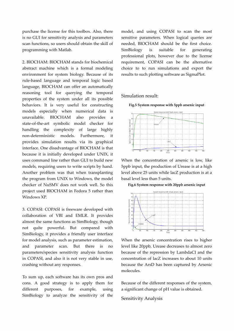
Simulation result:

Fig.5 System response with 5ppb arsenic input

When the concentration of arsenic is low, like 5ppb input, the production of Urease is at a high level above 25 units while lacZ production is at a basal level less than 5 units.

Fig.6 System response with 20ppb arsenic input

When the arsenic concentration rises to higher level like 20ppb, Urease decreases to almost zero because of the repression by LambdaCI and the concentration of lacZ increases to about 10 units because the ArsD has been captured by Arsenic molecules. Because of the different responses of the system, a significant change of pH value is obtained.

Sensitivity Analysis

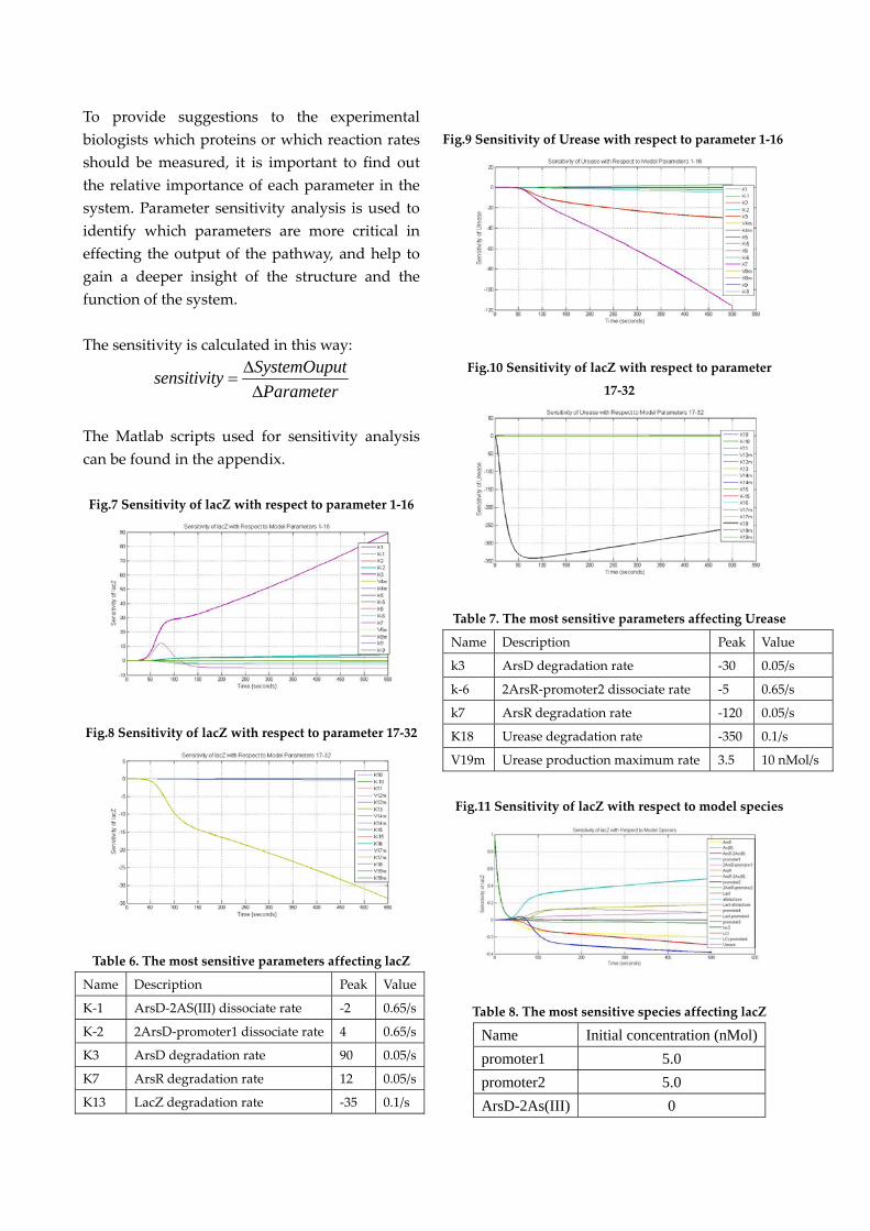
To provide suggestions to the experimental biologists which proteins or which reaction rates should be measured, it is important to find out the relative importance of each parameter in the system. Parameter sensitivity analysis is used to identify which parameters are more critical in effecting the output of the pathway, and help to gain a deeper insight of the structure and the function of the system. The sensitivity is calculated in this way:

SystemOuputsensitivityParameter

Δ=

Δ

The Matlab scripts used for sensitivity analysis can be found in the appendix. Fig.7 Sensitivity of lacZ with respect to parameter 1‐16

Fig.8 Sensitivity of lacZ with respect to parameter 17‐32

Table 6. The most sensitive parameters affecting lacZ

Name Description Peak Value

K‐1 ArsD‐2AS(III) dissociate rate ‐2 0.65/s

K‐2 2ArsD‐promoter1 dissociate rate 4 0.65/s

K3 ArsD degradation rate 90 0.05/s

K7 ArsR degradation rate 12 0.05/s

K13 LacZ degradation rate ‐35 0.1/s

Fig.9 Sensitivity of Urease with respect to parameter 1‐16

Fig.10 Sensitivity of lacZ with respect to parameter

17‐32

Table 7. The most sensitive parameters affecting Urease

Name Description Peak Value

k3 ArsD degradation rate ‐30 0.05/s

k‐6 2ArsR‐promoter2 dissociate rate ‐5 0.65/s

k7 ArsR degradation rate ‐120 0.05/s

K18 Urease degradation rate ‐350 0.1/s

V19m Urease production maximum rate 3.5 10 nMol/s

Fig.11 Sensitivity of lacZ with respect to model species

Table 8. The most sensitive species affecting lacZ

Name Initial concentration (nMol)promoter1 5.0 promoter2 5.0 ArsD-2As(III) 0

ArsD 25 ArsR 25

Fig.12 Sensitivity of lacZ with respect to model species

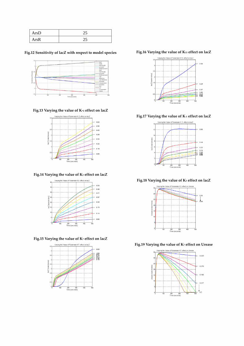
Fig.13 Varying the value of K‐2 effect on lacZ

Fig.14 Varying the value of K3 effect on lacZ



Fig.17 Varying the value of K‐1 effect on lacZ


Fig.19 Varying the value of K7 effect on Urease

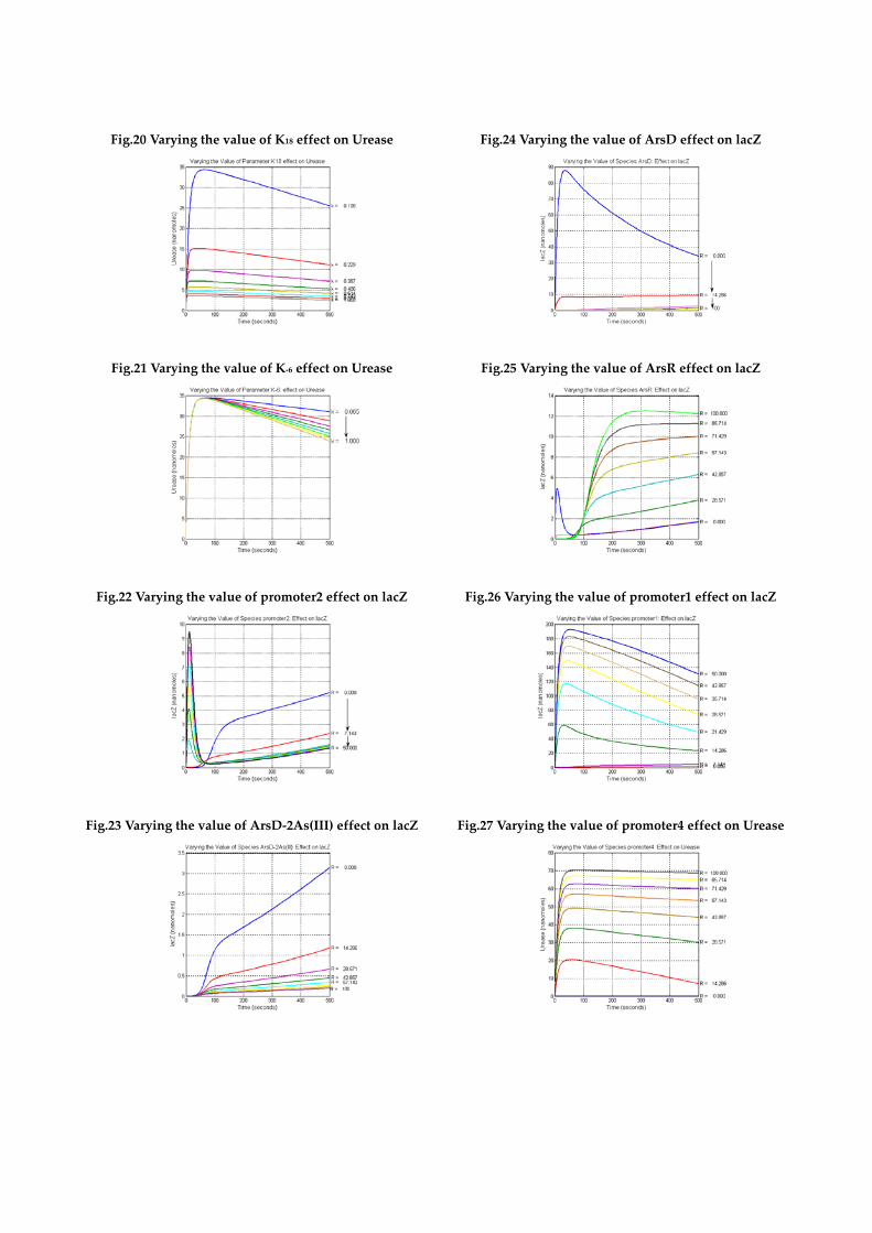
Fig.20 Varying the value of K18 effect on Urease

Fig.21 Varying the value of K‐6 effect on Urease

Fig.22 Varying the value of promoter2 effect on lacZ

Fig.23 Varying the value of ArsD‐2As(III) effect on lacZ

Fig.24 Varying the value of ArsD effect on lacZ

Fig.25 Varying the value of ArsR effect on lacZ

Fig.26 Varying the value of promoter1 effect on lacZ

Fig.27 Varying the value of promoter4 effect on Urease

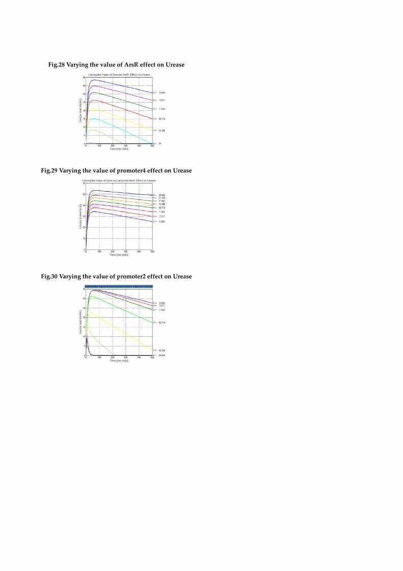
Fig.28 Varying the value of ArsR effect on Urease



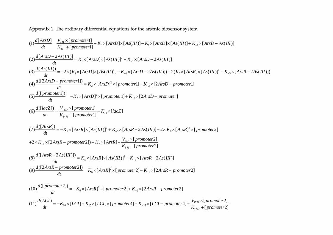
Appendix 1. The ordinary differential equations for the arsenic biosensor system

43 1 1

4

[ ] [ 1](1) [ ] [ ( )] [ ] [ ( )] [ ( )][ 1]

M

M

d ArsD V promoter K ArsD As III K ArsD As III K ArsD As IIIdt K promoter −

×= − × × − × × + × −

+

21 1

[ 2 ( )](2) [ ] [ ( )] [ 2 ( )]d ArsD As III K ArsD As III K ArsD As IIIdt −−

= × × − × −

2 21 1 5 5

( ( ))(3) 2 ( [ ] [ ( ) ] [ 2 ( )]) 2( [ ] [ ( )] [ 2 ( )])d Ar III K ArsD As III K ArsD As III K ArsR As III K ArsR As IIIdt − −= − × × × − × − − × × − × −

22 2

([2 1])(4) [ ] [ 1] [2 1]d ArsD promoter K ArsD promoter K ArsD promoterdt −−

= × × − × −

22 2

([ 1])(5) [ ] [ 1] [2 ]d promoter K ArsD promoter K ArsD promoterdt −= − × × + × −

1413

14

([ ]) [ 1](6) [ ][ 1]

M

M

d lacZ V promoter K lacZdt K promoter

×= − ×

+

2 25 5 6

86 7

8

([ ])(7) [ ] [ ( )] [ 2 ( )] 2 [ ] [ 2]

[ 2]2 [2 2]) [ ][ 2]

M

M

d ArsR K ArsR As III K ArsR As III K ArsR promoterdt

V promoterK ArsR promoter K ArsRK promoter

−

−

= − × × + × − − × × ×

×+ × × − − × +

+

25 5

([ 2 ( )])(8) [ ] [ ( )] [ 2 ( )]d ArsR As III K ArsR As III K ArsR As IIIdt −−

= × × − × −

26 6

([2 2])(9) [ ] [ 2] [2 2]d ArsR promoter K ArsR promoter K ArsR promoterdt −−

= × × − × −

26 6

([ 2])(10) [ ] [ 2] [2 2]d promoter K ArsR promoter K ArsR promoterdt −= − × × + × −

1716 15 15

17

( ) [ 2](11) [ ] [ ] [ 4] [ 4][ 2]

M

M

d LCI V promoterK LCI K LCI promoter K LCI promoterdt K promoter−

×= − × − × × + × − +

+

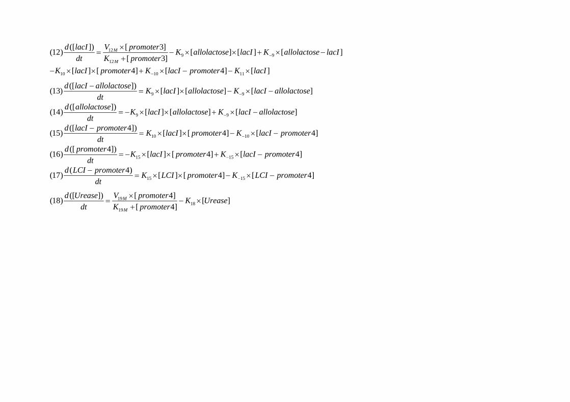
129 9

12

10 10 11

([ ]) [ 3](12) [ ] [ ] [ ][ 3]

[ ] [ 4] [ 4] [ ]

M

M

d lacI V promoter K allolactose lacI K allolactose lacIdt K promoter

K lacI promoter K lacI promoter K lacI

−

−

×= − × × + × −

+− × × + × − − ×

9 9([ ])(13) [ ] [ ] [ ]d lacI allolactose K lacI allolactose K lacI allolactose

dt −−

= × × − × −

9 9([ ])(14) [ ] [ ] [ ]d allolactose K lacI allolactose K lacI allolactose

dt −= − × × + × −

10 10([ 4])(15) [ ] [ 4] [ 4]d lacI promoter K lacI promoter K lacI promoter

dt −−

= × × − × −

15 15([ 4])(16) [ ] [ 4] [ 4]d promoter K lacI promoter K lacI promoter

dt −= − × × + × −

15 15( 4)(17) [ ] [ 4] [ 4]d LCI promoter K LCI promoter K LCI promoter

dt −−

= × × − × −

1918

19

([ ]) [ 4](18) [ ][ 4]

M

M

d Urease V promoter K Ureasedt K promoter

×= − ×

+

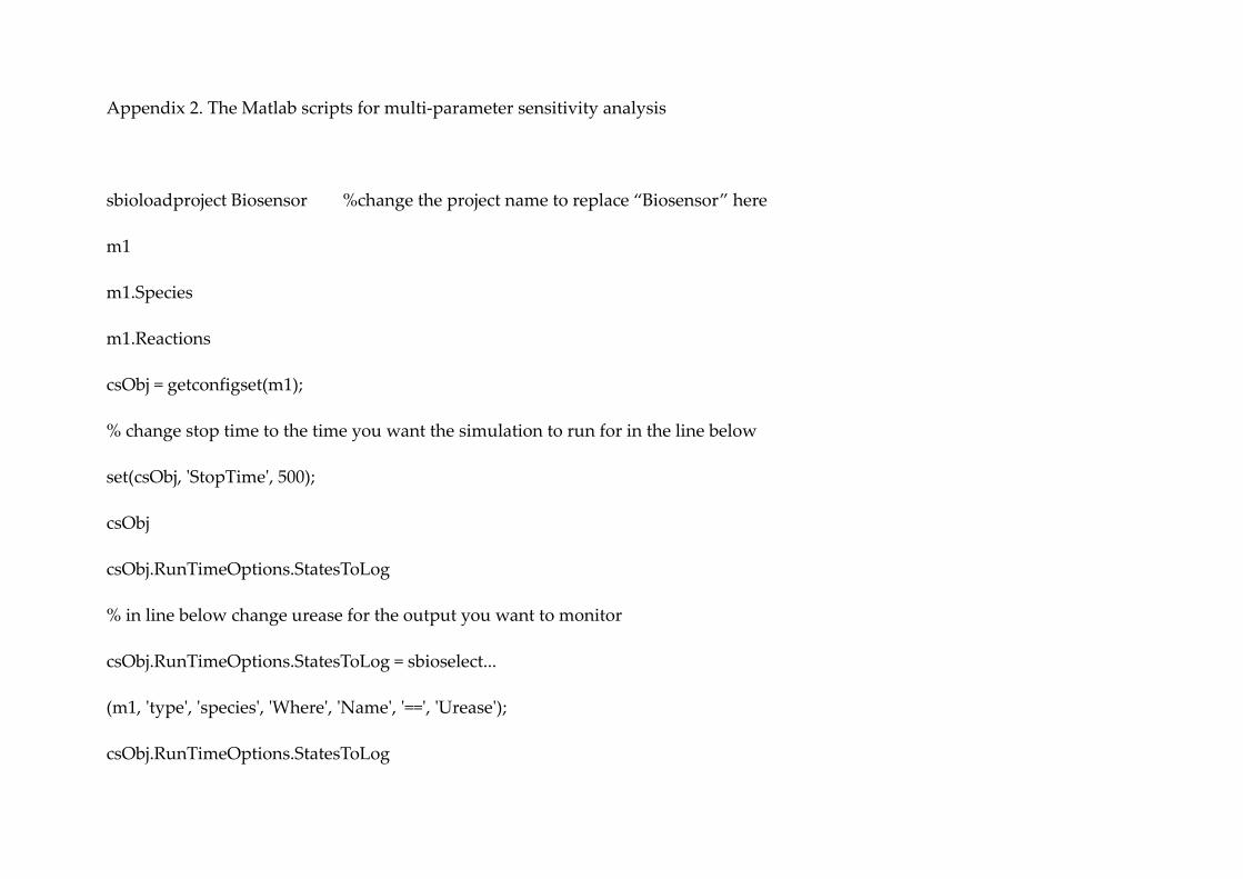
Appendix 2. The Matlab scripts for multi‐parameter sensitivity analysis

sbioloadproject Biosensor %change the project name to replace “Biosensor” here

m1

m1.Species

m1.Reactions

csObj = getconfigset(m1);

% change stop time to the time you want the simulation to run for in the line below

set(csObj, ʹStopTimeʹ, 500);

csObj

csObj.RunTimeOptions.StatesToLog

% in line below change urease for the output you want to monitor

csObj.RunTimeOptions.StatesToLog = sbioselect...

(m1, ʹtypeʹ, ʹspeciesʹ, ʹWhereʹ, ʹNameʹ, ʹ==ʹ, ʹUreaseʹ);


set(csObj.SolverOptions, ʹSensitivityAnalysisʹ, true);

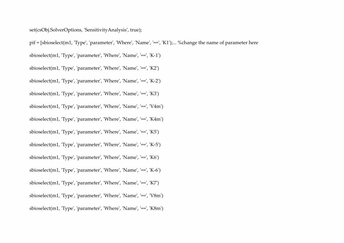
pif = [sbioselect(m1, ʹTypeʹ, ʹparameterʹ, ʹWhereʹ, ʹNameʹ, ʹ==ʹ, ʹK1ʹ);... %change the name of parameter here

sbioselect(m1, ʹTypeʹ, ʹparameterʹ, ʹWhereʹ, ʹNameʹ, ʹ==ʹ, ʹK‐1ʹ)

sbioselect(m1, ʹTypeʹ, ʹparameterʹ, ʹWhereʹ, ʹNameʹ, ʹ==ʹ, ʹK2ʹ)



sbioselect(m1, ʹTypeʹ, ʹparameterʹ, ʹWhereʹ, ʹNameʹ, ʹ==ʹ, ʹV4mʹ)

sbioselect(m1, ʹTypeʹ, ʹparameterʹ, ʹWhereʹ, ʹNameʹ, ʹ==ʹ, ʹK4mʹ)






sbioselect(m1, ʹTypeʹ, ʹparameterʹ, ʹWhereʹ, ʹNameʹ, ʹ==ʹ, ʹV8mʹ)

sbioselect(m1, ʹTypeʹ, ʹparameterʹ, ʹWhereʹ, ʹNameʹ, ʹ==ʹ, ʹK8mʹ)


sbioselect(m1, ʹTypeʹ, ʹparameterʹ, ʹWhereʹ, ʹNameʹ, ʹ==ʹ, ʹK‐9ʹ)];

set(csObj.SensitivityAnalysisOptions, ʹParameterInputFactorsʹ, pif);

set(csObj.SensitivityAnalysisOptions, ʹNormalizationʹ, ʹNoneʹ);

warning(ʹoffʹ, ʹMATLAB:divideByZeroʹ);

tsObj = sbiosimulate(m1);

[T, R, snames, ifacs] = sbiogetsensmatrix(tsObj);

size(R)

R2 = squeeze(R);

figure;

plot(T,R2);

% in lines below change the labels to suit the graph you want to draw

title(ʹSensitivity of Urease with Respect to Model Parameters 1‐16ʹ);

xlabel(ʹTime (seconds)ʹ);

ylabel(ʹSensitivity of Ureaseʹ);

Appendix 3. The Matlab script for Multi‐species sensitivity analysis

sbioloadproject Biosensor

m1

m1.Species

m1.Reactions




csObj






set(csObj.SolverOptions, ʹSensitivityAnalysisʹ, true);

sif = [sbioselect(m1, ʹTypeʹ, ʹspeciesʹ, ʹWhereʹ, ʹNameʹ, ʹ==ʹ, ʹArsDʹ);...

sbioselect(m1, ʹTypeʹ, ʹspeciesʹ, ʹWhereʹ, ʹNameʹ, ʹ==ʹ, ʹAs(III)ʹ);...

sbioselect(m1, ʹTypeʹ, ʹspeciesʹ, ʹWhereʹ, ʹNameʹ, ʹ==ʹ, ʹArsD‐2As(III)ʹ);...

sbioselect(m1, ʹTypeʹ, ʹspeciesʹ, ʹWhereʹ, ʹNameʹ, ʹ==ʹ, ʹpromoter1ʹ);...

sbioselect(m1, ʹTypeʹ, ʹspeciesʹ, ʹWhereʹ, ʹNameʹ, ʹ==ʹ, ʹ2ArsD‐promoter1ʹ);...

sbioselect(m1, ʹTypeʹ, ʹspeciesʹ, ʹWhereʹ, ʹNameʹ, ʹ==ʹ, ʹArsRʹ);...

sbioselect(m1, ʹTypeʹ, ʹspeciesʹ, ʹWhereʹ, ʹNameʹ, ʹ==ʹ, ʹArsR‐2As(III)ʹ);...


sbioselect(m1, ʹTypeʹ, ʹspeciesʹ, ʹWhereʹ, ʹNameʹ, ʹ==ʹ, ʹ2ArsR‐promoter2ʹ);...

sbioselect(m1, ʹTypeʹ, ʹspeciesʹ, ʹWhereʹ, ʹNameʹ, ʹ==ʹ, ʹLacIʹ);...

sbioselect(m1, ʹTypeʹ, ʹspeciesʹ, ʹWhereʹ, ʹNameʹ, ʹ==ʹ, ʹallolactoseʹ);...

sbioselect(m1, ʹTypeʹ, ʹspeciesʹ, ʹWhereʹ, ʹNameʹ, ʹ==ʹ, ʹLacI‐allolactoseʹ);...


sbioselect(m1, ʹTypeʹ, ʹspeciesʹ, ʹWhereʹ, ʹNameʹ, ʹ==ʹ, ʹLacI‐promoter4ʹ);...


sbioselect(m1, ʹTypeʹ, ʹspeciesʹ, ʹWhereʹ, ʹNameʹ, ʹ==ʹ, ʹlacZʹ);...

sbioselect(m1, ʹTypeʹ, ʹspeciesʹ, ʹWhereʹ, ʹNameʹ, ʹ==ʹ, ʹLCIʹ);...

sbioselect(m1, ʹTypeʹ, ʹspeciesʹ, ʹWhereʹ, ʹNameʹ, ʹ==ʹ, ʹLCI‐promoter4ʹ);...

sbioselect(m1, ʹTypeʹ, ʹspeciesʹ, ʹWhereʹ, ʹNameʹ, ʹ==ʹ, ʹUreaseʹ)

];

set(csObj.SensitivityAnalysisOptions, ʹSpeciesInputFactorsʹ, sif);


warning(ʹoffʹ, ʹMATLAB:divideByZeroʹ);

tsObj = sbiosimulate(m1);

[T, R, snames, ifacs] = sbiogetsensmatrix(tsObj);

size(R)

R2 = squeeze(R);

figure;

plot(T,R2);

% in lines below change the labels to suit the graph you want to draw

title(ʹSensitivity of Urease with Respect to Model Speciesʹ);

xlabel(ʹTime (seconds)ʹ);

ylabel(ʹSensitivity of Ureaseʹ);

Appendix 4. The Matlab lab script for parameter scan

sbioloadproject Tuning

m1

m1.Species

m1.Reactions




csObj




(m1, ʹtypeʹ, ʹspeciesʹ, ʹWhereʹ, ʹNameʹ, ʹ==ʹ, ʹpromoter1ʹ);

set(csObj.SolverOptions, ʹSensitivityAnalysisʹ, false);


h1 = figure;

ax1 = gca(h1);

% in next line change Vm4 to the name of the parameter you want to scan

p = sbioselect(m1, ʹTypeʹ, ʹparameterʹ, ʹNameʹ, ʹK2ʹ);

% in next line the first number is the lower limit and the second number the upper limit

% of your range and the last number is the number of scans in that range

s = linspace(1000, 100000, 8);

for k = s

set(p, ʹValueʹ, k);

[T,x,names] = sbiosimulate(m1);

str = sprintf( ʹ k = %8.3fʹ,k);

plot(ax1,T,x(:,1));

figure(h1);

hold on;

text(T(end),x(end,1),str);

end

axis([ax1], ʹsquareʹ);

% Change these lines to suit your data

title(ax1, ʹVarying the Value of Parameter K18 effect on Ureaseʹ);

xlabel(ax1, ʹTime (seconds)ʹ);

ylabel(ax1, ʹUrease (nanomoles)ʹ);

Appendix 5. The Matlab Script for species scan

sbioloadproject Biosensor

m1

m1.Species

m1.Reactions




csObj





set(csObj.SolverOptions, ʹSensitivityAnalysisʹ, false);


h1 = figure;

ax1 = gca(h1);

% in next line change Vm4 to the name of the parameter you want to scan

p = sbioselect(m1, ʹTypeʹ, ʹspeciesʹ, ʹNameʹ, ʹpromoter1ʹ);

% in next line the first number is the lower limit and the second number the upper limit

% of your range and the last number is the number of scans in that range

s = linspace(0, 50, 8);

for spR = s

set(p, ʹInitialAmountʹ, spR);

[T,x,names] = sbiosimulate(m1);

str = sprintf( ʹ R = %8.3fʹ,spR);

plot(ax1,T,x(:,1));

figure(h1);

hold on;

text(T(end),x(end,1),str);

end

axis([ax1], ʹsquareʹ);

% Change these lines to suit your data

title(ax1, ʹVarying the Value of Species promoter1: Effect on Ureaseʹ);

xlabel(ax1, ʹTime (seconds)ʹ);

ylabel(ax1, ʹUrease (nanomoles)ʹ);

Documents

Modeling the Arsenic Biosensor System - 2006.igem.org