Modeling stochastic perception error in the mean-excess traffic equilibrium model

Transportation Research Part B 45 (2011) 1619–1640

Contents lists available at ScienceDirect

Transportation Research Part B

journal homepage: www.elsevier .com/ locate/ t rb

Modeling stochastic perception error in the mean-excess trafficequilibrium model q

Anthony Chen a,⇑, Zhong Zhou b, William H.K. Lam c

a Department of Civil and Environmental Engineering, Utah State University, Logan, UT 84322-4110, USAb Citilabs, 1211 Miccosukee Road, Tallahassee, FL 32308, USAc Department of Civil and Structural Engineering, Hong Kong Polytechnic University, Hung Hom, Kowloon, Hong Kong

a r t i c l e i n f o

Article history:Received 4 September 2010Received in revised form 28 May 2011Accepted 28 May 2011

Keywords:Travel time reliabilityTravel time budgetMean-excess travel timePerception errorStochastic user equilibriumVariational inequality

0191-2615/$ - see front matter Published by Elseviedoi:10.1016/j.trb.2011.05.028

q This paper was presented at the 18th Internatio⇑ Corresponding author. Tel.: +1 435 797 7109; fa

E-mail address: [email protected] (A. Chen

a b s t r a c t

In this paper, we extend the a-reliable mean-excess traffic equilibrium (METE) model ofChen and Zhou (Transportation Research Part B 44(4), 2010, 493–513) by explicitly model-ing the stochastic perception errors within the travelers’ route choice decision processes. Inthe METE model, each traveler not only considers a travel time budget for ensuring on-timearrival at a confidence level a, but also accounts for the impact of encountering worsetravel times in the (1 � a) quantile of the distribution tail. Furthermore, due to the imper-fect knowledge of the travel time variability particularly in congested networks withoutadvanced traveler information systems, the travelers’ route choice decisions are basedon the perceived travel time distribution rather than the actual travel time distribution.In order to compute the perceived mean-excess travel time, an approximation methodbased on moment analysis is developed. It involves using the conditional moment gener-ation function to derive the perceived link travel time, the Cornish–Fisher AsymptoticExpansion to estimate the perceived travel time budget, and the Acerbi and TascheApproximation to estimate the perceived mean-excess travel time. The proposed stochasticmean-excess traffic equilibrium (SMETE) model is formulated as a variational inequality(VI) problem, and solved by a route-based solution algorithm with the use of the modifiedalternating direction method. Numerical examples are also provided to illustrate theapplication of the proposed SMETE model and solution method.

Published by Elsevier Ltd.

1. Introduction

Traffic equilibrium problem is one of the most critical and fundamental problems in transportation. Given the traveldemands between origin–destination (O–D) pairs (i.e., travelers), and travel cost function for each link of the transportationnetwork, the traffic equilibrium problem determines the equilibrium traffic flow pattern and various performance measuresof the network. Route choice model is inherently embedded in the traffic equilibrium problem to model individual routechoice decisions between various O–D pairs, while congestion is explicitly considered through the travel cost functions.Recently, travel time variability has emerged as an important topic due to its significant impacts on travelers’ route choicebehavior as observed by many empirical studies (Abdel-Aty et al., 1995; Small et al., 1999; Brownstone et al., 2003; Liu et al.,2004; de Palma and Picard, 2005; Fosgerau and Karlström, 2010; Fosgerau and Engelson, 2011). These studies revealed thattravelers indeed consider travel time variability as a risk in their route choice decisions since they do not know exactly when

r Ltd.

nal Symposium of Transportation and Traffic Theory, Hong Kong (Chen and Zhou, 2009).x: +1 435 797 1185.

).

http://dx.doi.org/10.1016/j.trb.2011.05.028

mailto:[email protected]

http://dx.doi.org/10.1016/j.trb.2011.05.028

http://www.sciencedirect.com/science/journal/01912615

http://www.elsevier.com/locate/trb

1620 A. Chen et al. / Transportation Research Part B 45 (2011) 1619–1640

they will arrive at the destination. Thus, they are interested in not only travel time saving but also risk reduction whenmaking their route choice. However, the traditional user equilibrium (UE) neglects travel time variability in the route choicedecision process. It adopts the expected travel time as the sole criterion for making route choice. Thus, it implicitly assumesall travelers to be risk-neutral. Moreover, it is well recognized that travelers may not have perfect knowledge about the roadtraffic condition particularly in congested network without advanced traveler information system (ATIS). Therefore, it isreasonable to incorporate the travelers’ perception error into the route choice decision process. However, similar to theUE model, the traditional stochastic user equilibrium (SUE) models (e.g., logit-based SUE model by Fisk (1980), C-logitSUE model by Cascetta et al. (1996) and Zhou et al. (2010), general SUE model by Daganzo (1982) and Sheffi and Powell(1982)) also neglect the effect of travel time variability in the route choice decision process. It adopts the expected perceivedtravel time as the sole criterion for making route choice; and hence, it also implicitly assumes all travelers are risk-neutral.

Typically, travel time variability can be represented by two different aspects: reliability aspect and unreliability aspect.The reliability aspect represents the acceptable travel time (or travel time budget), which is normally defined as the averagetravel time plus the acceptable additional time (or buffer time) needed to ensure the likelihood of on-time arrivals. The studyconducted by the Federal Highway Administration (2006) documented that travelers, especially commuters, do add a ‘‘buffertime’’ or ‘‘safety margin’’ to their expected travel time to ensure more frequent on-time arrivals when planning a trip. On theother hand, the unreliability aspect of travel time variability represents the late trips whose travel times are excessivelyhigher than the acceptable travel time. Based on the empirical data collected on the Netherlands freeways, travel timedistributions are not only very wide but also heavily skewed with a long tail (van Lint et al., 2008). The implication of thesepositively skewed travel time distributions has a significant impact on travelers’ route choice decisions. For example, it hasbeen shown that about 5% of the ‘‘unlucky drivers’’ incur almost five times as much delay as the 50% of the ‘‘fortunate drivers’’on the densely used freeway corridors in the Netherlands. In the United States, the cost of unexpected delay for truck freightis estimated to be 50–250% higher than the expected delay cost (FHWA, 2006). Recently, Franklin and Karlstrom (2009)estimated the ‘‘mean lateness’’ factor in the departure time choice model, and used it to conduct a benefit-cost analysisfor the roadway projects in Stockholm, Sweden. These empirical studies show that travel time distribution is not only heavilyskewed with a long fat tail, but also the consequences of these late trips may be much more serious than those of modestdelays, and can have a significant impact on both travelers and freight shippers and carriers. Therefore, to address thetravelers’ route choice behavior under an uncertain environment, both reliability and unreliability aspects of travel timevariability need to be considered simultaneously.

To consider the reliability aspect of travel time variability, the concept of travel time budget (TTB) has been adopted in theliterature. TTB is defined as the average travel time plus an extra time (or buffer time) such that the probability of completingthe trip within the TTB is no less than a predefined reliability threshold a. Uchida and Iida (1993) used the notion of effectivetravel time (i.e., mean travel time + safety margin) to model network uncertainty in the traffic assignment model. The safetymargin is defined as a function of travel time variability, which serves as a measure of risk averseness in their risk-basedtraffic assignment models. Lo et al. (2006) proposed a probabilistic user equilibrium (PUE) model to account for the effectsof within budget time reliability (WBTR) due to degradable links with predefined link capacity distributions. By assumingtravel time variability is induced by the travel demand fluctuation instead of capacity degradation, Shao et al. (2006a)proposed a demand driven travel time reliability-based user equilibrium (DRUE) model. Later, Lam et al. (2008) and Shaoet al. (2008) further extended this approach to model the impacts of adverse weather conditions on a road network withuncertainties in demand and supply.

On the other hand, to account for the unreliability aspect of travel time variability (i.e., unacceptable travel times), theconcept of schedule delay (SD) is adopted. It is defined as the difference between the chosen time of arrival and the officialwork start time (Small, 1982), used in conjunction with a disutility function to model the travel choice decision (Nolandet al., 1998; Noland, 1999). Watling (2006) proposed a late arrival penalized user equilibrium (LAPUE) model by incorporat-ing a schedule delay term to the disutility function to penalize late arrival for a fixed departure time. Siu et al. (2007) showedthat there is a relationship between the risk aversion coefficient of the TTB model and the SD cost.

However, note that both reliability-based and unreliability-based traffic equilibrium models above only consider one as-pect of travel time variability (i.e., either the reliability aspect using the concept of TTB or the unreliability aspect using theconcept of SD). To adequately describe travelers’ route choice decision process under travel time variability, both reliabilityand unreliability aspects should be explicitly considered. Recently, Chen and Zhou (2010) proposed a a-reliable mean-excesstraffic equilibrium (METE) model, where each traveler attempts to minimize his/her mean-excess travel time (METT), whichis defined as the conditional expectation of the travel time exceeding the TTB (see Fig. 1). As a route choice criterion, METTcan be regarded as a combination of the ‘‘buffer time’’ measure that ensures the reliability of on-time arrival, and the ‘‘tardytime’’ measure that represents the unreliability impacts of excessively late trips (Cambridge Systematics et al., 2003). Itincorporates both reliability and unreliability aspects of travel time variability to simultaneously address both questionsof ‘‘how much time do I need to allow?’’ and ‘‘how bad should I expect from the worse cases?’’ Therefore, travelers’ route choicebehavior can be considered in a more accurate and complete manner in a network equilibrium framework to reflect their riskpreferences under an uncertain environment.

To account for both reliability aspect of travel time variability and travelers’ perception error, Siu and Lo (2006) extendedthe PUE model to the stochastic travel time budget equilibrium (STTBE) model that considers two types of uncertainty intravelers’ daily commutes, i.e., uncertainty in the actual travel time due to random link degradations and perception errorvariations in the TTB due to imperfect information. Shao et al. (2006b) also extended the DRUE model to the reliability-based

0 5 10 15 20 25 30

Prob

abili

ty D

ensi

ty

0

0.1

0.2

0.3

0.4

0.5

0.6

0.7

0.8

0.9

1

Route Travel Time

Tra

vel T

ime

Rel

iabi

lity

Cumulative Probability

Probability Density

Confidence Level

Travel TimeBudget

Mean Excess Travel Time

Fig. 1. Illustration of the travel time budget and mean-excess travel time (Chen and Zhou, 2010).

Deterministic Perception Errors

Reliability -based Route Choice

Flow Dependent Network Congestion

Traffic Flow

TravelerNetwork

Perceived Travel Time Budget (PTTB)

Actual Travel Time Distribution

Travel Time Budget (TTB)

Fig. 2. Framework of reliability-based traffic equilibrium models with deterministic perception error.

A. Chen et al. / Transportation Research Part B 45 (2011) 1619–1640 1621

stochastic user equilibrium (RSUE) model that incorporates the randomness of link travel time from the daily demandvariation and travelers’ perception error on the TTB. Similar to the traditional logit-based SUE models (Dial, 1971; Fisk,1980; Cascetta et al., 1996; Zhou et al., 2010), they assumed the commonly adopted Gumbel variate as the random errorterm. Then, this random error term is added to the TTB to construct the perceived travel time budget (PTTB) as shown inFig. 2. According to Mirchandani and Soroush (1987), this kind of perception error is regarded as ‘‘deterministic’’, becauseit is independent of the stochastic travel time (i.e., actual travel time distribution).

Though a commonly adopted logit form can be acquired by this approach, it may not reflect the travelers’ perception ofthe random travel time appropriately. Under travel time variation, as discussed by Mirchandani and Soroush (1987), it ismore rational to assume that the traveler’s perception error is also dependent on the random travel time, i.e., the travelers’route choice decisions are based rather on the perceived travel time distribution than on the actual travel time distribution.Several recent empirical studies investigated methods to collect travelers’ perception on travel time variability, andconcluded that the perception of travel time unreliability plays an important role in making route choice decisions underuncertainty. Tseng et al. (2009) conducted a face-to-face in-depth interview to assess how travelers perceive travel timeunreliability. Peer et al. (2010) compared the perceived travel time distribution stated by the travelers in a survey to the

StochasticPerception Error

Route Choice Based on Both Reliability and Unreliability

Flow Dependent Network Congestion

Traffic Flow

Traveler

Network

Perceived Mean-excess Travel Time (PMETT)

Perceived Travel Time Distribution

Actual Travel Time Distribution

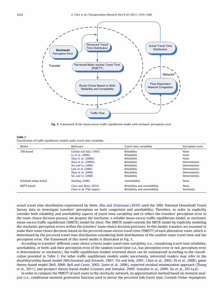
Fig. 3. Framework of the mean-excess traffic equilibrium model with stochastic perception error.

Table 1Classification of traffic equilibrium models under travel time variability.

Model Reference Travel time variability Perception error

TTB-based Uchida and Iida (1993) Reliability NoneLo et al. (2006) Reliability NoneShao et al. (2006a) Reliability NoneShao et al. (2006b) Reliability DeterministicSiu and Lo (2006) Reliability DeterministicLam et al. (2008) Reliability DeterministicShao et al. (2008) Reliability DeterministicSiu and Lo (2008) Reliability Deterministic

Schedule delay-based Watling (2006) Unreliability None

METT-based Chen and Zhou (2010) Reliability and unreliability NoneChen et al. (This paper) Reliability and unreliability Stochastic


actual travel time distribution experienced by them. Zhu and Srinivasan (2010) used the 2001 National Household TravelSurvey data to investigate travelers’ perception on both congestion and unreliability. Therefore, in order to explicitlyconsider both reliability and unreliability aspects of travel time variability and to reflect the travelers’ perception error inthe route choice decision process, we propose the stochastic a-reliable mean-excess traffic equilibrium model, or stochasticmean-excess traffic equilibrium (SMETE) model for short. The SMETE model extends the METE model by explicitly modelingthe stochastic perception errors within the travelers’ route choice decision processes. In this model, travelers are assumed tomake their route choice decisions based on the perceived mean-excess travel time (PMETT) of each alternative route, which isdetermined by the perceived travel time distribution considering both distributions of the random route travel time and theperception error. The framework of this novel model is illustrated in Fig. 3.

According to travelers’ different route choice criteria under travel time variability (i.e., considering travel time reliability,unreliability, or both) and their perception error of the random travel time (i.e., has perception error or not, perception erroris deterministic or stochastic), the traffic equilibrium models reviewed above can be summarized according to the classifi-cation provided in Table 1. For other traffic equilibrium models under uncertainty, interested readers may refer to thedisutility/utility-based model (Mirchandani and Soroush, 1987; Yin and Ieda, 2001; Chen et al., 2002; Di et al., 2008), gametheory-based model (Bell, 2000; Bell and Cassir, 2002; Szeto et al., 2006), expected residual minimization approach (Zhanget al., 2011), and prospect theory-based model (Connors and Sumalee, 2009; Sumalee et al., 2009; Xu et al., 2011a,b).

In order to compute the PMETT of each route in the stochastic network, an approximation method based on moment anal-ysis (i.e., conditional moment generation function used to derive the perceived link travel time, Cornish–Fisher Asymptotic


Expansion to estimate the PTTB, and Acerbi and Tasche Approximation to estimate the PMETT based on the PTTB) is devel-oped in this paper. This is the first attempt to integrate the traveler’s perception error, travel time reliability and unreliabilityinto a unified network equilibrium framework. It provides a more complete manner for considering travelers’ route choicedecisions to reflect their risk preferences under an uncertain environment and the potential applicability for solving practicalproblems.

The remainder of the paper is organized as follows. In Section 2, the concept of PMETT in a stochastic network withperception errors is introduced. Model formulation and solution properties are also provided. In Section 3, a route-based traf-fic assignment algorithm based on the modified alternating direction method is provided to determine the equilibrium flowpattern. In Section 4, two numerical examples are presented to demonstrate the characteristics of the proposed SMETEmodel and its comparison to other related stochastic user equilibrium models. Finally, conclusions are drawn and recom-mendations for future research are given in Section 5.

2. Model and formulation

This section describes the stochastic mean-excess traffic equilibrium (SMETE) model for determining the equilibriumflow pattern under stochastic travel times and perception errors. Assumptions are provided first, followed by the definitionsof mean-excess travel time and perceived mean-excess travel time, derivation of the perceived mean-excess route travel time,the SMETT conditions, the variational inequality formulation, and its qualitative properties.

2.1. Assumptions

Consider a strongly connected network [N, A], where N and A denote the sets of nodes and links, respectively. Let R and Sdenote the subsets of N for which travel demand qrs is generated from origin r 2 R to destination s 2 S, and let f rs

p denote theflow on route p 2 Prs, where Prs is a set of routes from origin r to destination s. Let Ta represent the random travel time on linka 2 A, which is parameterized by link flow Va. Consequently, the travel time on route p 2 Prs between origin r and destinations is also a random variable that can be expressed as

Trsp ¼

Xa2A

Tadrspa; 8 p 2 Prs; r 2 R; s 2 S; ð1Þ

where D ¼ ½drspa� denotes the route–link incidence matrix, drs

pa ¼ 1 if route p from origin r to destination s uses link a, and 0,otherwise.

In this study, travelers, especially commuters, are assumed to have the ability to learn the travel time variability throughtheir past experiences. Then, they incorporate this knowledge into their daily route choice decisions to reach a habitualequilibrium (Lo and Tung, 2003; Lo et al., 2006). However, due to the imperfect knowledge about the network condition,travelers’ perception errors have to be incorporated into their route choice decision process. Therefore, under an uncertainenvironment, it is reasonable to assume that travelers make their route choice decisions based on the perceived travel timedistribution rather than the actual one. This can be illustrated in Fig. 4, which shows a hypothetical travel time distributionand the corresponding travel time distribution perceived by travelers. Due to the differences between the actual travel timedistribution (depicted in the dotted line) and the perceived travel time distribution (depicted in the solid line), the travelers’route choice decisions could be quite different.

In the following, we give specific assumptions on the perception error used to develop the stochastic mean-excess trafficequilibrium model with probabilistic travel times and perception errors:

Travel Time Distribution

Perceived Travel Time Distribution

Travel Time

Dis

tribu

tion

Den

sity

Fig. 4. Actual travel time distribution and perceived travel time distribution.


Assumption 1. The perception error distribution of an individual traveler for a segment of road with a unit travel time isN(l, r2), where N(l, r2) denotes a normal distribution with mean l and variance r2.

Assumption 2. Traveler’s perception errors are independent for non-overlapping route segments.

Assumption 3. Travelers’ perception errors are mutually independent over the population of travelers.

Note that, in our assumptions above, the parameters l and r2 of the normal distribution N(l, r2) are predefined anddeterministic. This is distinct from the assumptions proposed by Mirchandani and Soroush (1987), where the parametersl and r2 are also random variables with given distributions. Though the random parameters l and r2 have the advantageto represent characteristics that vary from one individual to another or from day to day of the same individual, it requires themodel to be appropriately aggregated. Such aggregation adds complexity to the model and may significantly increase thecomputational efforts. For example, the Monte Carlo simulation, which is known to be a time-consuming procedure, hasbeen adopted by the seminal work of Mirchandani and Soroush (1987) to account for the randomly distributed parameters(l and r2) in the estimation of perceived route disutility. Recently, Xu et al. (2011b) also used the normal distribution tomodel the perceived travel time distribution in the cumulative prospect theory-based route choice model.

In this study, we assume all travelers come from a single group and have similar attributes. This kind of aggregationsimplification has been widely adopted in various travel demand models, such as mode choice, destination choice, and routechoice models (see, e.g., Sheffi, 1985; Oppenheim, 1995). Therefore, based on the assumptions in this study, computationallyintensive simulation can be avoided, and efficient moment-based analysis of the perceived travel time distribution and newroute choice criterion can be derived.

According to Assumptions 1–3, the traveler’s perception error on route p and link a can be denoted as ersp jTrs

pand eajTa

,which are conditional on the stochastic route/link travel time Trs

p and Ta, respectively. Then, the perceived travel timeeT rsp ðeT aÞ can be rationally assumed as the actual travel time Trs

p (Ta) plus the perception error ersp jTrs

pðeajTa

Þ, and the followingequation is satisfied
eT rs
p ¼Trsp þ ers

p jTrsp; 8p 2 Prs; r 2 R; s 2 S; ð2Þ

¼Xa2A

Ta þ eajTa

� �drs

pa; ð3Þ

¼Xa2A

eT adrspa; ð4Þ

From the above equations, it can be seen that travelers’ perceived travel time is in fact dependent on the actual travel time. Inother words, the perceived distribution of the travel time is conditioned on the actual distribution of the stochastic travel time.This distinguishes our approach from the logit-based SUE approach adopted in the recently developed reliability-based trafficequilibrium models (Siu and Lo, 2006; Shao et al., 2006b), where the perception error term is independent of the stochastictravel time, because it was assumed to be an independently and identically distributed (IID) Gumbel variate. In the next sec-tion, we will see how the travelers hedge against travel time variability and make their route choice decisions to reach a long-term habitual equilibrium state while recognizing the perception of actual travel time distribution is subject to error.

2.2. Route choice criterion under an uncertain environment

According to Mirchandani and Soroush (1987), travelers making route choice decisions under an uncertain environmentcan be categorized into three groups according to their attitudes toward risk (i.e., risk-prone, risk-neutral, and risk-averse). Inthe traditional UE and SUE models, travelers are assumed to be risk-neutral since they make their route choice decisionssolely based on the expected (perceived) travel time. However, recent empirical studies (Brownstone et al., 2003; Liuet al., 2004; de Palma and Picard, 2005) revealed that most travelers are actually risk-averse. They are willing to pay apremium to avoid congestion and minimize the associated risk.

By considering the travel time reliability requirement, travelers are searching for a route such that the corresponding TTBallows for on-time arrival with a predefined confidence level a (Lo et al., 2006; Shao et al., 2006a). Meanwhile, they are alsoconsidering the impacts of excessively late arrival (i.e., the unreliable aspect of travel time variability) and its explicit link tothe travelers’ preferred arrival time in the route choice decision process (Watling, 2006). Therefore, it is reasonable for trav-elers to choose a route such that the travel time reliability requirement (i.e., acceptable travel time defined by TTB) isensured most of the time and the expected unreliability impact (i.e., unacceptable travel time exceeding TTB) is minimized.This trade-off between the reliable and unreliable aspects of travel time variability in travelers’ route choice decision processwas represented by the mean-excess route travel time defined by Chen and Zhou (2010) as follows:

Definition 1. The mean-excess travel time grsp ðaÞ for route p 2 Prs between origin r and destination s with a predefined

confidence level a is equal to the conditional expectation of the travel time exceeding the corresponding route TTB nrsp ðaÞ, i.e.,

grsp ðaÞ ¼ E Trs

p jTrsp P nrs

p ðaÞh i

; 8p 2 Prs; r 2 R; s 2 S; ð5Þ


where E[�] is the expectation operator, and nrsp ðaÞ is the travel time budget on route p from origin r to destination s defined by

the travel time reliability chance constraint at a confidence level a in Eq. (6):

nrsp ðaÞ ¼ min njPrðTrs

p 6 nÞP an o

; ð6Þ

¼ E Trsp

� �þ crs

p ðaÞ; 8p 2 Prs; r 2 R; s 2 S; ð7Þ

where crsp ðaÞ is the extra time added to the mean travel time as a ‘buffer time’ to ensure more frequent on-time arrivals at the

destination under the travel time reliability requirement at a confidence level a. Note that Eq. (7) is exactly the definition ofthe TTB defined by Chen and Ji (2005), Lo et al. (2006), and Shao et al. (2006a).

To incorporate the travelers’ perception error, similar to Definition 1 above, we can define the perceived mean-excesstravel time ~grs

p ðaÞ as follows:

Definition 2. The perceived mean-excess travel time ~grsp ðaÞ for route p 2 Prs between origin r and destination s with a

predefined confidence level a is equal to the conditional expectation of the perceived travel time exceeding thecorresponding perceived route travel time budget ~nrs

p ðaÞ, i.e.,

~grsp ðaÞ ¼ E eT rs

p jeT rsp P ~nrs

p ðaÞh i

; 8p 2 Prs; r 2 R; s 2 S; ð8Þ

where eT rsp is the perceived travel time on route p between origin r and destination s, and ~nrs

p ðaÞ is the perceived travel timebudget (PTTB), defined by

~nrsp ðaÞ ¼ minf~njPrðeT rs

p 6~nÞP ag; ð9Þ

¼ E eT rsp

� �þ ~crs

p ðaÞ; 8p 2 Prs; r 2 R; s 2 S; ð10Þ

where ~crsp ðaÞ is the perceived ‘‘buffer time’’ added to the perceived mean travel time to ensure the predefined travel time

reliability at a confidence level a.According to the definition above, it can be seen that if the perceived route travel time distribution f ðeT rs

p Þ is known (to berelaxed later using the approximation scheme developed in this paper), the perceived mean-excess travel time ~grs

p ðaÞ can berepresented as:

~grsp ðaÞ ¼

11� a

ZeT rs

p P~nrsp ðaÞ

eT rsp f ðeT rs

p ÞdðeT rsp Þ: ð11Þ

Moreover, Eq. (11) can be restated as:

~grsp ðaÞ ¼ ~nrs

p ðaÞ þ E eT rsp � ~nrs

p ðaÞjeT rsp P ~nrs

p ðaÞh i

: ð12Þ

Therefore, the PMETT can be decomposed into two individual components. The first component is exactly the PTTB of routep, which reflects the perceived reliability aspect of travel time variability (or acceptable risk) allowed by the travelers at aconfidence level a. The second component can be regarded as a kind of ‘‘perceived expected excess delay’’ for choosingthe current route to reflect the perceived unreliability aspect of travel time variability (i.e., perceived trip time exceedingthe acceptable travel time defined by PTTB or unacceptable risk). Clearly, the PMETT incorporates both reliable and unreli-able aspects of the travel time variability and perception error into the route choice decision process to address the questionsof ‘‘how much time do I need to allow?’’ and ‘‘how bad should I expect from the worse cases?’’ when making a route choicedecision.

2.3. Perceived mean-excess route travel time

In the literature, several possible travel time distributions have been suggested to describe the travel time variation underan uncertain environment. For example, exponential and uniform travel time distributions were adopted in Noland andSmall (1995) for studying the morning commuting problem. A family of distributions known as the ‘‘Johnson curves’’ wasstudied by Clark and Watling (2005) to model the total network travel time under random demand. Gamma-type distribu-tions were tested by Fan and Nie (2006) in the stochastic optimal routing problem. Lognormal distribution was considered inZhou and Chen (2008) to model demand uncertainty in the traffic equilibrium problem. Normal distribution was also used byLo et al. (2006), Siu and Lo (2006), and Shao et al. (2006a,b) to derive the mean and variance of link travel time introduced byeither link capacity degradation or demand fluctuation. A mixture of normal distribution was also suggested in Watling(2006) to allow for a more flexible control over the right-hand tail and better fit of the data. In this study, the SMETE modeland its VI formulation are proposed in a generic sense, that is, flexible travel time probability density functions are allowed.They provide a simple, convenient representation of risk, which fits quite well to the way that travelers assess their triptimes and risks, and make their route choice decisions accordingly.

To determine the PMETT of a route, the cumulative distribution function (CDF) is required. However, in real applications,this information is generally unknown. Even the link travel time distributions are given, it may still be difficult to derive the


route travel time distribution without further assumptions. This becomes even more complicated when the travelers’perception error is incorporated and the perceived travel time distribution needs to be derived. To overcome this difficulty,an approximation scheme based on moment analysis is adopted in this study to estimate the PMETT without the need toknow the explicit form of the perceived route CDF. This approximation scheme involves three steps: (1) derivation of theperceived link and route travel times using the conditional moment generation function and the concept of cumulants,(2) derivation of the PTTB using the Cornish–Fisher Asymptotic Expansion, and (3) derivation of the PMETT using Acerbiand Tasche Approximation.

2.3.1. Step 1: Derivation of the perceived link and route travel timesFrom Assumption 1, the perception error of an individual traveler for a segment of a road with a unit travel time, denoted

by e|T=1, follows N(l, r2). Moreover, according to Assumption 2, the travel time on link a is the sum of independent unit traveltimes. Therefore, the conditional perception error for link a with deterministic travel time t0

a is normally distributed as:

eajTa¼t0a� N l 1þ 1þ � � � þ 1|fflfflfflfflfflfflfflfflfflfflfflffl{zfflfflfflfflfflfflfflfflfflfflfflffl}

¼t0a

0B@1CA; r2 1þ 1þ � � � þ 1|fflfflfflfflfflfflfflfflfflfflfflffl{zfflfflfflfflfflfflfflfflfflfflfflffl}

¼t0a

0B@1CA

264375 ¼ Nðlt0

a ; r2t0aÞ ð13Þ

with conditional moment generating function (MGF)

Mea jTa¼t0aðsÞ ¼ exp lt0

asþ r2t0as2

2

� �¼ exp st0

a lþ r2s2

� � ; ð14Þ

where s is a real number.From the conditional MGF above, we can derive the first to fourth cumulants jð1Þa ;jð2Þa ;jð3Þa and jð4Þa of the perceived link

travel time distribution, respectively (see Appendix A for the derivations). In this study, we assume the perceived link traveltimes are independent (i.e., a typical assumption made in the analytical transportation network reliability literature, see Loand Tung, 2003; Lo et al., 2006; Zhou and Chen, 2008; Chen and Zhou, 2010; Ng and Waller, 2010) to simplify the derivationfrom the cumulants of perceived link travel times to the cumulants of perceived route travel times. Therefore, from theadditive property of the cumulants, we have

jrsp

� �ðiÞ¼Xa2A

jðiÞa drspa; 8p 2 Prs; r 2 R; s 2 S; i ¼ 1;2;3;4: ð15Þ

Note that, in reality, the link travel times may not be truly independent due to the network topology or the sources ofvariations. The source of link travel times correlation can be classified into two types: network topology and route propaga-tion (aggregation from link travel time to route travel time). As to the modeling of link correlation, some recent studies canbe adopted. For the route propagation-related correlation, we may use the covariance of link flows (e.g., stemmed from atravel demand distribution) and a polynomial link performance function to obtain the first four moments of actual/perceivedlink travel times. Then, a multinomial expansion may be used to obtain the first four moments of perceived route travel times(see, e.g., Clark and Watling, 2005; Lam et al., 2008). Also, the convolution method (e.g., Nie, 2011) is another alternative thatcan deal with the route propagation-related correlation. In addition, the concept of copula (Nelsen, 1999; Cherubini et al.,2004) can be used to handle the correlation due to network topology. Therefore, how to relax this assumption would beof interest for further study.

2.3.2. Step 2: Derivation of the PTTBNow, we are able to use the following Cornish–Fisher Asymptotic Expansion (Cornish and Fisher, 1937) to estimate the

PTTB ~nrsp ðaÞ. The Cornish–Fisher Asymptotic Expansion is a well-known and widely used method to approximate the percen-

tile of a random variable from its moments. Depending on the highest order of moments under consideration (e.g., thesecond-order moment), we may have different versions for this expansion. In this study, we use the first four momentsto approximate the percentile of the perceived route travel time (i.e., perceived travel time budget) as follows:

~nrsp ðaÞ � �nrs

p ðaÞ ¼ E½eT rsp � þ wpðaÞ � V ½eT rs

p �; 8p 2 Prs; r 2 R; s 2 S; ð16Þ

where E½eT rsp � and V ½eT rs

p � denote the expected value and standard deviation of the perceived route travel time eT rsp , respectively,

which are obtained from

E½eT rsp � ¼ ðjrs

p Þð1Þ; 8p 2 Prs; r 2 R; s 2 S; ð17Þ

V ½eT rsp � ¼ ðjrs

p Þð2Þ

h i1=2; 8p 2 Prs; r 2 R; s 2 S; ð18Þ

and

wpðaÞ ¼ U�1ðaÞ þ ð1=6Þ ðU�1ðaÞÞ2 � 1h i

Sp þ ð1=24Þ ðU�1ðaÞÞ3 � 3U�1ðaÞh i

Kp � ð1=36Þ 2ðU�1ðaÞÞ3 � 5U�1ðaÞh i

S2p; ð19Þ


where U�1( � ) is the inverse of the standard normal CDF, while Sp and Kp are the theoretical skewness and kurtosis of theperceived route travel time distribution, respectively, which are obtained from

Sp ¼ðjrs

p Þð3Þ

ðjrsp Þð2Þ

h i3=2 ; 8p 2 Prs; r 2 R; s 2 S; ð20Þ

Kp ¼ðjrs

p Þð4Þ

ðjrsp Þð2Þ

h i2 ; 8p 2 Prs; r 2 R; s 2 S: ð21Þ

Note that Eq. (16) is related to the 3rd and 4th moments of the perceived route travel time as shown in Eq. (19). In general,higher order moments will increase the accuracy of estimation. Jaschke (2002) provided several qualitative and quantitativeproperties of the Cornish–Fisher Expansion in the context of Delta–Gamma-Normal approximations to the computation ofVaR. The author concluded that ‘‘in many practical situations, its actual accuracy is more than sufficient, and the Cornish–Fisher-approximation can be computed faster (simpler) than other methods like numerical Fourier inversion’’ despite some qualitativedeficiencies. Their results also showed that ‘‘the higher order approximations have increasing accuracy near the normaldistribution, but become less reliable far from the normal distribution.’’ The error for a 99%-VaR computed with the Cornish–Fisher approximation using up to the fourth cumulant was about 2 � 10�6 times the standard deviation, which is more thansufficient for most real-world problems.

If only the perceived reliability aspect of travel time variability is considered, i.e., the user equilibrium is based on thePTTB, the approach above can be considered as an extension of Shao et al. (2006b) and Siu and Lo (2006). That is, insteadof adding a Gumbel random term as the perception error to the TTB, where the TTB itself is computed based on the actualtravel time distribution and the Gumbel distributed perception error is independent of the stochastic travel time, we com-pute the PTTB according to the perceived travel time distribution, which integrates the distribution of the uncertain traveltime and perception error together.

2.3.3. Step 3: Derivation of the PMETTIn order to consider both reliability and unreliability aspects of travel time variability, and to incorporate the travelers’

perception error, the PMETT is adopted as a route choice criterion in this study. However, it is generally difficult to directlyestimate the PMETT using Eq. (11), because the analytical form of the perceived route travel time distribution f ðeT rs

p Þ is gen-erally unknown. However, the PMETT can be approximated as follows. Let FðeT Þ be the CDF of route perceived travel time eT(to facilitate the presentation, we drop the superscript and subscript). Set Y ¼ FðeT Þ or eT ¼ F�1ðYÞ. We can rewrite ~gðaÞ as

~gðaÞ ¼ 11� a

Z 1

Fð~nðaÞÞF�1ðsÞds

Recall that Fð~nðaÞÞ is the confidence level a whose percentile is ~nðaÞ. Thus, Fð~nðaÞÞ ¼ a, and F�1(s) is the s-percentile, i.e.,F�1ðsÞ ¼ ~nðsÞ. Using Proposition 3.2 in Acerbi and Tasche (2002), the PMETT can be redefined as the following equivalent form:

~grsp ðaÞ ¼

11� a

Z 1

a

~nrsp ðsÞds: ð22Þ

Consequently, we have

~grsp ðaÞ � �grs

p ðaÞ ¼1

1� a

Z 1

a

�nrsp ðsÞds: ð23Þ

Note that the integral in the right-hand side of Eq. (23) can be readily computed by many efficient numerical methods, e.g.,adaptive algorithms under various quadrature rules (Stoer and Bulirsch, 2002). Thus, from the analysis above, we are able toestimate the PMETT without the need to know the explicit form of the perceived route travel time CDF.

2.4. SMETE conditions and variational inequality formulation

By adopting the PMETT as a route choice criterion, the stochastic mean-excess traffic equilibrium (SMETE) conditions canbe described as an extension of the user equilibrium principle (Wardrop, 1952) as follows:

Definition 3. Let ~g denote the PMETT vector ð. . . ; ~grsp ; . . . ÞT , f denote the route-flow vector ð. . . ; f rs

p ; . . . ÞT , and ~prs denote theminimal PMETT between O–D pair (r, s). The stochastic a-reliable mean-excess traffic equilibrium state is reached byallocating the O–D demands to the network such that no traveler can improve his/her perceived mean-excess travel time byunilaterally changing routes. In other words, all used routes between each O–D pair have equal perceived mean-excess travel time,and no unused route has a lower perceived mean-excess travel time, i.e., the following conditions hold:

~grsp ðf �Þ � ~prs

¼ 0 ifðf rsp Þ�> 0

P 0 ifðf rsp Þ� ¼ 0

(; 8 p 2 Prs; r 2 R; s 2 S ð24Þ


Then, the SMETE model can be formulated as a variational inequality problem VI(~g;X) as follows.Find a vector f⁄ 2X, such that

~gðf �ÞTðf � f �ÞP 0; 8f 2 X; ð25Þ
where X represents the feasible route set defined by Eqs. (26)–(28):
qrs ¼Xp2Prs

f rsp ; 8 r 2 R; s 2 S; ð26Þ

va ¼Xr2R

Xs2S

Xp2Prs

f rsp drs

pa; 8 a 2 A; ð27Þ

f rsp P 0; 8 p 2 Prs; r 2 R; s 2 S; ð28Þ

where (26) is the travel demand conservation constraint; (27) is a definitional constraint that sums up all route flows thatpass through a given link a; and (28) is a non-negativity constraint on the route flows.

The following Propositions give the equivalence of the VI formulation and the SMETE model as well as the existence of theequilibrium solutions.

Proposition 1. Assume the perceived mean-excess route travel time function ~gðf Þ is positive, then the solution of the VIproblem (25) is equivalent to the equilibrium solution of the SMETE problem.

Proof. Note that f⁄ is a solution of the VI problem if and only if it is a solution of the following linear program

minf2X

~gðf �ÞT f : ð29Þ

By considering the primal-dual optimality conditions of (29), we have

f rs�p � ð~grs

p ðf �Þ � ~prsÞ ¼ 0; 8 p 2 Prs; r 2 R; s 2 S; ð30Þ~grs

p ðf �Þ � ~prs P 0; 8 p 2 Prs; r 2 R; s 2 S; ð31Þ

Eqs. (26) and (28). It is easy to see the SMETE conditions (24) are satisfied. This completes the proof. h

Proposition 2. Assume the perceived mean-excess route travel time function ~gðf Þ is positive and continuous, then the SMETEproblem has at least one solution.

Proof. According to Proposition 1, we only need to consider the equivalent VI formulation. Note that the feasible set X isnonempty and convex. Furthermore, according to the assumption, the mapping ~gðf Þ is continuous. Thus, the VI problem(25) has at least one solution (Facchinei and Pang, 2003). This completes the proof. h

In this study, the travelers are assumed to be risk-averse and concerned with both reliability and unreliability compo-nents introduced by travel time variability. Consider the relationship of the perceived link and route travel times in Eqs.(2)–(4), the assumptions of the perception error distribution (Assumptions 1–3), and the definition of the PMETT in Eq.(11), it is reasonable to give the positive and continuous assumption of the function ~gðf Þ as in the above propositions.Consequently, the validity of the VI formulation and the existence of the solution are ensured.

However, note that the solution to the SMETE problem is not unique in general. The reason is that the underlying map-ping (i.e., PMETT) in the VI formulation is generally nonadditive (i.e., the route cost is not simply the sum of the costs onthe links that constitute that route). For example, TTB or PTTB can be considered as a combination of the mean and stan-dard deviation (SD) of travel time. As is well known, SD does not hold under the additive property. Thus, the route TTB orPTTB cannot be decomposed into the sum of generalized link costs on this route. This nonadditivity property also appliesto the PMETT of the SMETE model in this paper. As is well known, in order to guarantee the solution uniqueness, the map-ping in the VI problem is required to be strictly monotone. This requirement is typically not satisfied in most traffic equi-librium models under uncertainty (see Lo et al., 2006; Shao et al., 2006a,b, Chen and Zhou, 2010). How to select a‘‘meaningful and reasonable’’ equilibrium solution from the set of equilibrium solutions will be a valuable research direc-tion in the future.

3. Solution algorithm

As mentioned above, the PMETT in the SMETE problem is nonadditive in general. Therefore, a number of well-knownalgorithms developed for the traditional traffic assignment problem, such as the Frank–Wolfe algorithm, cannot be appliedto solve the SMETE problem. In order to deal with the nonadditive route cost structure, a route-based solution algorithm isneeded (Bernstein and Gabriel, 1997; Chen et al., 2001; Gabriel and Bernstein, 1997; Lo and Chen, 2000). By exploring thespecial structure of the SMETE model, a modified alternating direction (MAD) method (Han, 2002) is adopted in this study for


solving the VI problem in Eq. (25). The MAD method is a projection-based algorithm, whose main idea can be brieflysummarized as below.

First, we attach a Lagrangian multiplier vector y to the demand conservation constraints (26). Therefore, the VI problem(25) can be reformulated as the following equivalent VI problem, denoted by VI(F, K).

Find x⁄ 2 K, such that

Fðx�ÞTðx�x�ÞP 0; 8x 2 K; ð32Þ

where

x ¼f

y

� �; FðxÞ ¼

~gðf Þ �KT yKf � q

!;K ¼ Rn

þ � Rk; ð33Þ

where K denotes the OD-route incidence matrix, q denotes the demand vector (. . ., qrs, . . .)T, n represents the total number ofroutes, and k is the total number of O–D pairs.

This transformation makes the MAD method attractive, because a projection on the new feasible region K (which is just anonnegative orthant) is much easier than on the original set X. That is, in each iteration, the MAD algorithm does not need tosolve a time-consuming convex program, but only needs to perform two orthogonal projections onto the nonnegativeorthant and some function evaluations. Furthermore, a self-adaptive stepsize updating scheme is embedded in the algo-rithm, where the stepsize is automatically decided according to the information calculated in the previous iterations (i.e.,route flows and PMETTs). These features make the MAD method efficient and robust. For more detailed steps about theMAD method, we refer to Han (2002) and Zhou et al. (2007)). One note of caution is that the convergence of the MAD methodrequires the monotonicity of the VI(F, K), which may not be satisfied. Therefore, the proposed algorithm should be regardedas a heuristic approach in that case. However, the solution obtained from this algorithm is indeed an optimal solution, be-cause it satisfies the PMETT-based equilibrium condition as well as the conservation constraint.

The remaining complication is how to generate the route set in real applications. Two approaches proposed by Lo andChen (2000) and Chen et al. (2001) can be considered here. The first approach works with a set of predefined routes, whichcould be derived from personal interviews and hence constitutes a set of likely used routes; the second approach is to use aheuristic column generation procedure to generate PMETT routes. Zhou and Chen (submitted for publication) proposed aheuristic algorithm for finding a-reliable mean-excess routes. This approach may also be extended to find routes with theminimum PMETT. In the numerical illustrations, we assume a set of working routes is available. Future work will be explor-ing and developing a more efficient algorithm for finding the minimum PMETT routes and combining it as a columngeneration procedure in the proposed solution algorithm.

4. Illustrative examples

The purpose of this section is to illustrate and appraise the essential ideas of the SMETE model. There are two numericalexamples in this study. The first example is used to illustrate the detailed derivations of PMETT using moment analysis, toanalyze the characteristics of PMETT, and to examine the effects of the perception error on various route choice models (i.e.,the logit-based SUE model by Fisk (1980), the reliability-based SUE model by Shao et al. (2006b) and Siu and Lo (2006), andthe METE model by Chen and Zhou (2010)). The second example is used to analyze the convergence characteristics of theMAD method and the sensitivities of the SMETE model with respect to variations of demand level, confidence level, andperception error.

4.1. A three-parallel route network

As shown in Fig. 5, the first example is a simple network with three parallel routes (here links and routes are identical).There is one O–D pair (1, 2) with 1 unit demand. The link capacities are all assumed to be 1, and the mean and variance of the

1 2

Link 1

Link 2

Link 3

Fig. 5. Three-parallel route network.


link free-flow travel time in minute for the three links are (11, 4), (9, 9), and (10, 6), respectively. The travel time for eachindividual link is assumed to be calculated from the following Bureau of Public Road (BPR) function:

Ta ¼ T0a 1þ 0:15

Va

Ca

� �2 !

; 8 a 2 A; ð34Þ

where Ta; T0a ;Va, and Ca are the travel time, free-flow travel time, flow, and capacity of link a, respectively. Note that the travel

time variability may come from any combination of the variables T0a (random link free-flow travel time), Va (random link flow

induced by day-to-day travel demand variation), and/or Ca (link capacity subject to stochastic degradation). For simplicity,following Mirchandani and Soroush (1987), we assume that the probabilistic link travel time Ta only comes from therandomness of the link free-flow travel time T0

a . Here, we assume the random link free-flow travel time follows the Gammadistribution, i.e., T0

a � Cðs; hÞ, with the following probability density function (PDF):

f ðT0a ; s; hÞ ¼ ðT

0aÞ

s�1 e�T0a=h

hsCðsÞ ; ð35Þ

where s is the shape parameter, h is the scale parameter, and C(s) is the gamma function of s. Gamma distributions are quiteflexible to mimic a broad range of commonly used nonnegative probability distributions, such as Exponential, Weibull, andLognormal distributions, thus convenient for modeling a wide range of random processes. Without loss of generality, weassume the confidence level of all travelers is 90% and the perception error distribution of a unit travel time follows N(0, 0.2).

4.1.1. Estimation of the PMETTFirst, we illustrate the proposed approximation scheme based on moment analysis for estimating the PMETT without the

need to know the explicit form of the perceived route travel time distribution. Without loss of generality, we assume that theinitial flows on links 1–3 are 0.2, 0.2 and 0.6, respectively. If the travelers have perfect knowledge of the network condition,they will be able to perceive the travel time distribution accurately (i.e., no perception error). Therefore, according to Eqs.(5)–(7), it is easy to compute the METT for each individual route:

g121 ð0:9Þ ¼ 14:86;g12

2 ð0:9Þ ¼ 15:05;g123 ð0:9Þ ¼ 15:52: ð36Þ

However, due to the imperfect knowledge of the network condition, the travelers may not be able to perceive the actual tra-vel time distribution exactly (see Fig. 4). Hence, it is necessary to incorporate their perception error into the route choicedecisions. Based on the assumption of Gamma distributed free-flow link travel time in Eq. (35) and the BPR link cost functionin Eq. (34), the first to fourth moments of the link travel time distribution can be computed as follows:

E½T1� ¼ 11:07; E½T2� ¼ 9:05; E½T3� ¼ 10:54; ð37ÞE½ðT1Þ2� ¼ 126:50; E½ðT2Þ2� ¼ 91:08; E½ðT3Þ2� ¼ 117:76; ð38ÞE½ðT1Þ3� ¼ 1492:45; E½ðT2Þ3� ¼ 1007:93; E½ðT3Þ3� ¼ 1390:10; ð39ÞE½ðT1Þ4� ¼ 18153:40; E½ðT2Þ4� ¼ 12167:70; E½ðT3Þ4� ¼ 17288:94: ð40Þ

Then, the first to fourth moments of the perceived travel time distribution can be computed according to Appendix A:

E½eT 1� ¼ 11:07; E½eT 2� ¼ 9:05; E½eT 3� ¼ 10:54; ð41ÞE½ðeT 1Þ2� ¼ 128:72; E½ðeT 2Þ2� ¼ 92:89; E½ðeT 3Þ2� ¼ 119:87; ð42ÞE½ðeT 1Þ3� ¼ 1568:36; E½ðeT 2Þ3� ¼ 1062:58; E½ðeT 3Þ3� ¼ 1460:75; ð43ÞE½ðeT 1Þ4� ¼ 19959:52; E½ðeT 2Þ4� ¼ 13388:14; E½ðeT 3Þ4� ¼ 18971:19: ð44Þ

Consequently, the first to fourth cumulants of the perceived link travel time distribution can be derived as follows:

jð1Þ1 ¼ 11:07; jð1Þ2 ¼ 9:05; jð1Þ3 ¼ 10:54; ð45Þjð2Þ1 ¼ 6:26; jð2Þ2 ¼ 10:92; jð2Þ3 ¼ 8:77; ð46Þjð3Þ1 ¼ 5:39; jð3Þ2 ¼ 23:79; jð3Þ3 ¼ 12:43; ð47Þjð4Þ1 ¼ 7:29; jð4Þ2 ¼ 78:39; jð4Þ3 ¼ 26:91: ð48Þ

Since the routes and links are identical in this example, according to Eq. (15), we have

ðj12p ÞðiÞ ¼ jðiÞa ; 8a ¼ p ¼ 1;2;3; i ¼ 1;2;3;4: ð49Þ

By considering Eqs. (20) and (21), the skewness and kurtosis of the perceived route travel time distribution can be derived as:

S1 ¼ 0:34; S2 ¼ 0:66; S3 ¼ 0:48; ð50ÞK1 ¼ 0:19; K2 ¼ 0:66; K3 ¼ 0:35: ð51Þ


Based on the Cornish–Fisher (1937) Asymptotic Expansion in Eq. (16), the perceived travel time budget (PTTB) can be esti-mated as:

~n121 ð0:9Þ ¼ 14:35; ~n12

2 ð0:9Þ ¼ 13:45; ~n123 ð0:9Þ ¼ 14:45: ð52Þ

Then, by adopting Eq. (23), we can finally obtain the PMETT of each route

~g121 ð0:9Þ ¼ 15:77; ~g12

2 ð0:9Þ ¼ 15:61; ~g123 ð0:9Þ ¼ 16:24: ð53Þ

Compared to the actual METTs in Eq. (36), the PMETTs at a confidence level of 0.9 for the three routes are generally higher.

4.1.2. Analysis of the PMETTSecond, we examine the characteristics of the PMETT. According to the definition of the PMETT, it can be decomposed into

three different components, i.e., the perceived mean travel time (PMTT), the perceived buffer time (PBT), and the perceivedexpected excess delay (PEED). This can be demonstrated more clearly in Fig. 6. Here, the perceived expected excess delay de-scribes the impacts from the unreliability aspect of travel time variability on travelers’ route choice decisions, and the sum-mation of the other two components (PMTT and PBT) gives the PTTB that represents the travel time reliability requirement.From Fig. 6, we can see that travelers on route 3 may experience a higher perceived expected excess delay than those on route1 when the 10% worse cases happen (i.e., (1 � a) quantile of worse travel times in the distribution tail), even though thesetwo routes have similar PTTB. These worse cases may be due to various sources, such as severe incidents, bad weather con-ditions, and special events. Therefore, for travelers who are concerned with not only the travel time reliability, but also theunreliability of encountering worse travel times, they may prefer route 1 over route 3, which has a lower PMETT.

The impacts on travelers’ route choice decision by considering both travel time reliability and unreliability can be furtherillustrated in Fig. 7. It shows the percentage of each component (i.e., PMTT, PBT, and PEED) corresponding to the PMETTs.From Fig. 7, we can see that the unreliability aspect of travel time variability is as significant as the reliability aspect on trav-elers’ route choice decision. Here, the PEEDs (unreliability aspect) occupy 9%, 14%, and 11%, respectively, on the three routes.Furthermore, the results show that the sum of the reliability and unreliability aspects of travel time variability has nearly30–42% impacts on travelers’ route choice decisions under an uncertain environment. Therefore, both reliability andunreliability aspects of travel time variability should be considered in the route choice model.

04

812

16

Route 1

Route 2

Route 3

Minutes

(1.79

PEED + PBT +PMTT )

PMETT3.91

10.54

4.4

9.05

3.28

16.24

15.61

15.77

11.07

2.16

1.42

PTTB

=

Fig. 6. Analysis of the characteristics of PMETT.

21%

70%

9%28%

14%

58%

24%11%

65%

PEED

PBT

PMTT PMTT

PEED

PBT

PEED

PBT

PMTTRoute 3Route 2Route 1

Fig. 7. Proportion of each component in the PMETTs.

Table 2Equilibrium results of the METE and SMETE models.

Model Route # Route flow METT PMETT

METE 1 0.37 15.08 15.992 0.23 15.08 15.653 0.40 15.08 15.80

SMETE 1 0.24 14.90 15.812 0.36 15.25 15.813 0.41 15.09 15.81

Route 1Route 2

Route 3

0

0.2

0.4

0.6

Equi

libriu

m F

low

SUE (8.92)RSUE (12.89)SMETE (15.81)

0.58

0.23 0.24

0.12

0.43

0.36

0.300.34

0.41

Fig. 8. Comparison of the different stochastic user equilibrium models.


4.1.3. Effects of the perception error on various route choice modelsThird, we analyze the effects of the perception error on various route choice models. Initially, we compare the

equilibrium results of the METE and SMETE models. The results are shown in Table 2. The ‘Route Flow’ column gives theequilibrium route flow pattern of each model. The ‘METT’ and ‘PMETT’ columns provide the METT and the PMETT basedon the equilibrium route flow pattern of each model, respectively. For example, the ‘PMETT’ column of the METE modelprovides the PMETT of each route under the equilibrium route flows of the METE model given the same perception errordistribution adopted in the SMETE model. Similarly, the ‘METT’ column of the SMETE model shows the METT of each routeunder the computed equilibrium route flows of the SMETE model given no perception error. To check the validity of theresults, we examine two conditions for each model: travel demand conservation constraints and equilibrium conditions.As expected, both conditions are satisfied: the route flows sum up to the O–D travel demands and the corresponding equi-librium measures (METT for the METE model and PMETT for the SMETE model) of all used routes for each O–D pair are equaland minimal. From Table 2, it is clear that the perception error affects the equilibrium route flow patterns. For example, if theperception error is incorporated, route 1 will have the highest PMETT value under the equilibrium route flows of the METEmodel. Therefore, travelers using route 1 have incentives to switch from route 1 to route 2 or route 3. On the other hand,under the equilibrium state of the SMETE model, if travelers are able to estimate the distribution of the stochastic travel timeaccurately, they will switch from route 2 to other routes in order to acquire a lower METT.

Then, we compare the SMETE model with the traditional logit-based SUE model (Fisk, 1980) and the reliability-based SUEmodel (Siu and Lo, 2006; Shao et al., 2006b). The equilibrium results are shown in Fig. 8, where we use SUE and RSUE torepresent the traditional logit-based SUE model and the reliability-based SUE model, respectively. The values in the legendare the equilibrium measures for each model, e.g., the equilibrium PMETT for the SMETE model is 15.81.

From Fig. 8, we can see that the equilibrium route flow pattern obtained from the SMETE model is significantly differentfrom those obtained by Fisk’s logit-based SUE model and the reliability-based SUE model. In particular, the differences can beexplained by the following reasons: (1) the SMETE model explicitly considers both reliability and unreliability aspects oftravel time variability, while the RSUE model only considers the reliability aspect of travel time variability and the traditionallogit-based SUE model totally ignores the travel time variability. Therefore, the value of the equilibrium measure of the RSUEmodel (i.e., PTTB) is higher than the route travel time of the SUE model due to the extra buffer time added to ensure on-timearrival, and the equilibrium PMETT of the SMETE model is higher than the PTTB of the RSUE model due to its furtherconsideration of the impacts of the unreliable late trips in the distribution tail; (2) the travelers’ perception error in theSMETE model depends on the distribution of the stochastic travel time. However, in the SUE and RSUE models, the percep-tion error is independent of the actual travel time distribution, and is just considered as a separate cost added to theexpected travel time and TTB, respectively. In fact, comparing with the SUE and RSUE models, our model gives much lesstraffic flow on route 2, even it has the lowest mean route travel time. This is reasonable because the risk-averse travelers


would avoid the routes with higher travel time variation even if the expected travel time does not increase much. Therefore,the travelers would rather travel through route 1 and route 3 to get a higher confidence of on-time arrival, and at the sametime, to avoid the possible delays that are potentially much higher than the TTB in the (1 � a) quantile of the distribution tail.

4.2. Nguyen–Dupuis network

In this example, we use the well-known Nguyen–Dupuis (N–D) network (1984) to further demonstrate the SMETE modeland solution algorithm. Specifically, we analyze the convergence characteristics of the MAD algorithm, the impacts ofdemand level, confidence level, and perception error variation on the SMETE model. The N–D network, shown in Fig. 9,contains 13 nodes, 19 directed links, 4 O–D pairs, and 25 routes. The link-route incidence relationship is shown in Table3. In this example, we assume the travel time variability is induced by the lognormal distributed travel demand. The meanvalues of the base travel demands of O–D pairs (1, 2), (1, 3), (4, 2), and (4, 3) are 200, 400, 300, and 100, respectively, and thevariance–mean ratio (VMR) are all equal to 0.5. We adopt the standard BPR function TaðVaÞ ¼ t0

a 1þ 0:15ðVa=CaÞ4h i

as the linkperformance function. The fixed link free-flow travel time t0

a and capacity Ca are listed in Table 4. Because the source ofuncertainty between Sections 4.1 and 4.2 is different, we provide the derivations of the first to fourth moments of the actuallink travel time distribution in Appendix B for completeness.

For simplicity, we further assume all travelers have the same confidence level of 90%. The perception error is normallydistributed with the mean of 0.5 and variance of 0.2. For the stopping criterion, we adopt the equilibrium conditions inEq. (24) (i.e., the percentage route cost difference weighted by route flows as a residual error) to directly measure theconvergence of the MAD algorithm. The tolerance error is set to be 1e�8. The results reported in the next two sectionsare tested on a personal laptop computer with 2.00 G Pentium (R) Dual-Core processor and 1.86G RAM.

1 122

5 6 7 8

11 2

4

9 10

313

1

3 5 7 9

12 14 15

19

1718

6 8 10 114

13 16Origin

Destination

Fig. 9. Nguyen–Dupuis (N–D) network.

Table 3Link-route incidence relationship.

O–D Route Link sequence O–D Route Link sequence

(1, 2) 1 2-18-11 (1, 3) 9 1-6-13-192 1-5-7-9-11 10 1-5-7-10-163 1-5-7-10-15 11 1-5-8-14-164 1-5-8-14-15 12 1-6-12-14-165 1-6-12-14-15 13 2-17-7-10-166 2-17-7-9-11 14 2-17-8-14-167 2-17-7-10-158 2-17-8-14-15

(4, 2) 15 4-12-14-15 (4, 3) 20 4-13-1916 3-5-7-9-11 21 4-12-14-1617 3-5-7-10-15 22 3-6-13-1918 3-5-8-14-15 23 3-5-7-10-1619 3-6-12-14-15 24 3-5-8-14-16

25 3-6-12-14-16

Table 4Link characteristics.

Link From To Free-flow travel time Capacity Link From To Free-flow travel time Capacity

1 1 5 7 800 11 8 2 9 5502 1 12 9 400 12 9 10 10 5503 4 5 9 200 13 9 13 9 6004 4 9 12 800 14 10 11 6 7005 5 6 3 350 15 11 2 9 5006 5 9 9 400 16 11 3 8 3007 6 7 5 800 17 12 6 7 2008 6 10 13 250 18 12 8 14 4009 7 8 5 250 19 13 3 11 600

10 7 11 9 300

0 10 20 30 40 50 60 70 80 90 1000

0.02

0.04

0.06

0.08

0.1

0.12

Iterations

Res

idua

l Err

or

Fig. 10. Convergence curve of the MAD algorithm.

0 10 20 30 40 50 60 70 80 90 1000

50

100

150

200

Iterations

Rou

te F

low

Flow on route 1=181.8160

Flow on route 2=18.1840Routes 3-8

Fig. 11. Evolution of the route flows for O–D pair (1, 2) during the iteration process.


4.2.1. Convergence characteristic of the MAD algorithmThe convergence characteristic of the MAD algorithm is shown in Fig. 10. As can be seen, the residual error drops sharply

in the early iterations and stabilizes after the 30th iteration. The superior performance of the MAD method is attributed tothe self-adaptive step size strategy. The step size automatically adjusts itself according to the route flows and PMETTs in theprevious iterations.

To further demonstrate the convergence characteristics of the MAD algorithm, without loss of generality, we investigatethe evolution of the route flows and PMETTs connecting O–D pair (1, 2) during the iteration process in Figs. 11 and 12,respectively. These figures demonstrate the same convergence characteristics in equilibrating the route flows to reach anequilibrium solution. At equilibrium, the used routes (route 1 and route 2) have the same minimum PMETT 53.4658, whilethe unused routes (routes 3–8) have higher PMETTs. Also note that the flows on the two used routes sum up to the totaltravel demand between O–D pair (1, 2), i.e., f 1;2

1 þ f 1;22 ¼ 181:816þ 18:184 ¼ 200 ¼ q1;2.

In order to examine the impact of the stopping error on the computational effort, we test the tolerance error from 1e�1 to1e�10 with an interval of one order of magnitude. The number of iterations and CPU time required to converge to therequired accuracy are shown in Fig. 13. From this figure, we can see that both iteration and CPU time increase linearly withrespect to the order of magnitude of the tolerance error. This implies the computational effort of the MAD algorithm ismodest for solving the SMETE model.

10 20 30 40 50 60 70 80 90 10045

50

55

60

65

70

75

80

IterationsP

ME

TT

Route 1

Route 2PMETT=53.4658

Routes 3 - 8

Fig. 12. Evolution of the route METTs for O–D pair (1, 2) during the iteration process.

1 2 3 4 5 6 7 8 9 100

40

80

120

160

200

Error(1e-)

Iter

atio

ns

1 2 3 4 5 6 7 8 9 100

2

4

6

8

10

CP

U T

ime

(sec

)

Iterations

CPU Time

Fig. 13. Computational efforts for different tolerance error levels.

0.50.6

0.70.8

0.90.95

0.40.8

1.21.6

2.050

52

54

56

58

60

Confidence Level (CL)Demand Level (DL)

PM

ET

T

52

54

56

58

60

DL=2.0,CL=0.5,PMETT=56.99 DL=1.6,CL=0.8,

PMETT=54.96

DL=2.0,CL=0.95,PMETT=60.46

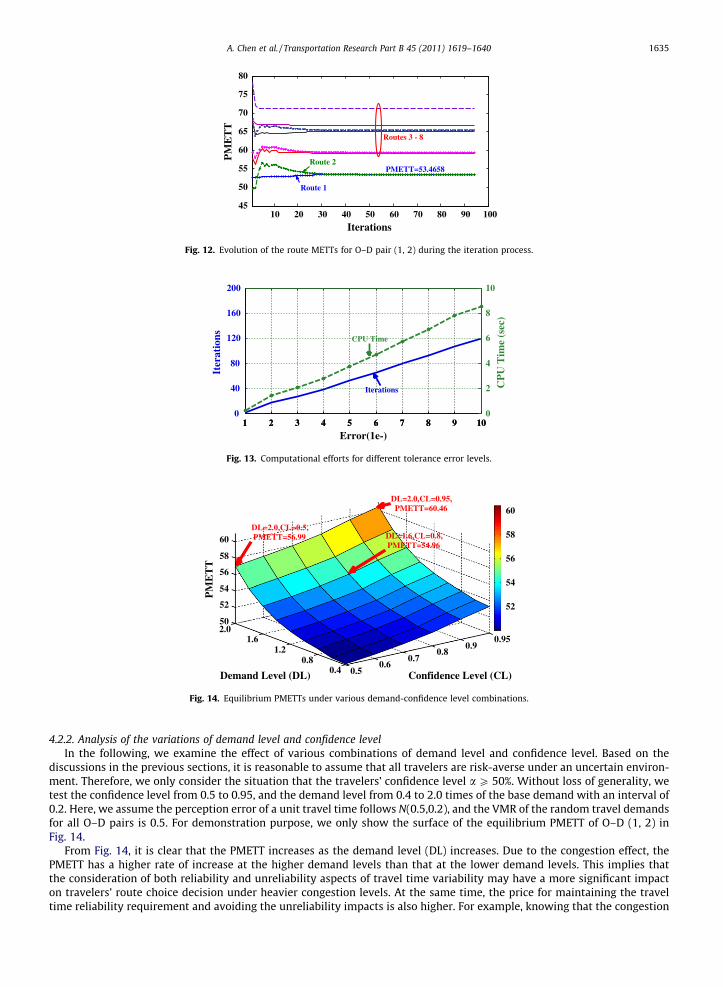
Fig. 14. Equilibrium PMETTs under various demand-confidence level combinations.


4.2.2. Analysis of the variations of demand level and confidence levelIn the following, we examine the effect of various combinations of demand level and confidence level. Based on the

discussions in the previous sections, it is reasonable to assume that all travelers are risk-averse under an uncertain environ-ment. Therefore, we only consider the situation that the travelers’ confidence level a P 50%. Without loss of generality, wetest the confidence level from 0.5 to 0.95, and the demand level from 0.4 to 2.0 times of the base demand with an interval of0.2. Here, we assume the perception error of a unit travel time follows N(0.5,0.2), and the VMR of the random travel demandsfor all O–D pairs is 0.5. For demonstration purpose, we only show the surface of the equilibrium PMETT of O–D (1, 2) inFig. 14.

From Fig. 14, it is clear that the PMETT increases as the demand level (DL) increases. Due to the congestion effect, thePMETT has a higher rate of increase at the higher demand levels than that at the lower demand levels. This implies thatthe consideration of both reliability and unreliability aspects of travel time variability may have a more significant impacton travelers’ route choice decision under heavier congestion levels. At the same time, the price for maintaining the traveltime reliability requirement and avoiding the unreliability impacts is also higher. For example, knowing that the congestion

34 36 38 40 42 44 460.5

0.6

0.7

0.8

0.9

1

PMETT

Con

fide

nce

Lev

el (

α )

µ=0

σ2=0.2

σ2=0.5

σ2=0.8

37.14 39.75 41.63

(a) μ = 0

42 44 46 48 50 520.5

0.6

0.7

0.8

0.9

1

PMETT

Con

fide

nce

Lev

el (

α )

µ=0.2

σ2=0.2

σ2=0.5

σ2=0.8

43.67 46.28 48.16

(b) μ = 0.2

50 52 54 56 58 60 620.5

0.6

0.7

0.8

0.9

1

PMETT

Con

fide

nce

Lev

el (

α )

µ=0.5

σ2=0.2

σ2=0.5

σ2=0.8

53.47 56.08 57.96

(c) μ = 0.5

Fig. 15. Equilibrium PMETTs under various parameter values of the perception error distribution.


is severe, travelers have to depart earlier to ensure more frequent on-time arrival and to minimize the associated risk ofencountering excessively high delay. Furthermore, we can see that the equilibrium PMETT is increasing while the confidencelevel increases. This is to be expected since travelers need to budget extra time in order to satisfy a higher travel time reli-ability requirement given by the increasing a value.

4.2.3. Analysis of the variations of perception errorFinally, we investigate the impact of the parameters of perception error distribution N(l, r2). Here, the expected O–D

demands are fixed at the base case, the VMR is 0.5, and the confidence level is 90%. l and r2 are varied as follows: (a)l = 0, 0.2, and 0.5, (b) r2 = 0.2, 0.5, and 0.8. Again, only the equilibrium PMETT of O–D (1, 2) under different l and r2 of


the perception error distribution is shown in Fig. 15. From this figure, we can see that the PMETT increases as l and r2

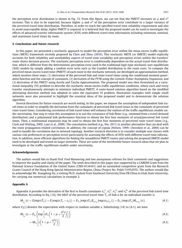
increase. This is also to be expected, because higher l and r2 of the perception error contribute to a larger variance ofthe perceived travel time distribution. Therefore, in order to reach the specified travel time reliability requirement and alsoto avoid unacceptable delay, higher PMETT is required. It is believed that the proposed model can be used to investigate theeffects of advanced traveler information system (ATIS) with different travel time information including minimum, nominal,and maximum travel times by route.

5. Conclusions and future research

In this paper, we presented a stochastic approach to model the perception error within the mean excess traffic equilib-rium (METE) framework recently proposed by Chen and Zhou (2010). This stochastic METE (or SMETE) model explicitlyaccounts for both reliability and unreliability aspects of travel time variability and perception errors within the travelers’route choice decision process. The stochastic perception error is conditionally dependent on the actual travel time distribu-tion, which is different from the deterministic perception error used in the traditional logit-type stochastic user equilibrium(SUE) models by simply adding a random error term such as the Gumbel distribution to the route costs. To compute theperceived mean-excess travel time (PMETT) of each route in the stochastic network, we developed an approximation method,which involves three steps: (1) derivation of the perceived link and route travel times using the conditional moment gener-ation function and the concept of cumulants, (2) derivation of the PTTB using the Cornish–Fisher Asymptotic Expansion, and(3) derivation of the PMETT using Acerbi and Tasche Approximation. The proposed model was then formulated as a varia-tional inequality (VI) problem to describe the stochastic mean-excess traffic equilibrium conditions, where each and everytraveler simultaneously attempts to minimize individual PMETT. A route-based solution algorithm based on the modifiedalternating direction method was adopted to solve the equivalent VI problem. Illustration examples with simple smallnetworks were also presented to highlight the essential ideas of the proposed model and to demonstrate the solutionalgorithm.

Several directions for future research are worth noting. In this paper, we impose the assumption of independent link tra-vel times in order to simplify the derivation from the cumulants of perceived link travel times to the cumulants of perceivedroute travel times. Considering correlation of link travel times will enhance the realism of the traffic equilibrium models un-der uncertainty. One way to relax this assumption is to use the covariance of link flows (e.g., stemmed from a travel demanddistribution) and a polynomial link performance function to obtain the first four moments of actual/perceived link traveltimes. Then, a multinomial expansion may be used to obtain the first four moments of perceived route travel times (e.g.,Clark and Watling, 2005; Lam et al., 2008). The convolution method (e.g., Nie, 2011) is another alternative that can deal withthe route propagation-related correlation. In addition, the concept of copula (Nelsen, 1999; Cherubini et al., 2004) can beused to handle the correlation due to network topology. Another research direction is to consider multiple user classes withvarious risk preferences or perception errors particularly for assessing the effects of ATIS with different travel time informa-tion. In addition, more efficient algorithms for finding the nonadditive PMETT routes and solving the proposed SMETE modelneed to be developed and tested on larger networks. These are some of the worthwhile future research ideas that we plan toinvestigate in the traffic equilibrium models under uncertainty.

Acknowledgements

The authors would like to thank Prof. Fred Mannering and two anonymous referees for their comments and suggestionsto improve the quality and clarity of the paper. The work described in this paper was supported by a CAREER Grant from theNational Science Foundation of the United States (CMS-0134161) and an earmarked competitive grant from the ResearchGrants Council of the Hong Kong Special Administrative Region, China (Project No. PolyU 5195/07E). The authors would liketo acknowledge Mr. Xiangdong Xu, a visiting Ph.D. student from Southeast University from PR China to Utah State University,for carrying out numerical calculations in example 2.

Appendix A

Appendix A provides the derivation of the first to fourth cumulants jð1Þa ;jð2Þa ;jð3Þa and jð4Þa of the perceived link travel timedistribution. According to Eq. (14), the MGF of the perceived travel time eT a of link a for an individual traveler is

MeT aðsÞ ¼ E½expðseT aÞ� ¼ Efexp½sðTa þ eaÞ�g ¼ ETafexpðsTaÞEea jTa

½expðseajTaÞ�g ¼ ETafexpðsTaÞMea jTa

ðsÞg: ðA:1Þ

where Ex[�] denotes the expectation with respect to random variable x. Substituting (14) to (A.1), we have

MeT aðsÞ ¼ ETa exp sTa 1þ lþ r2s

2

� � � �: ðA:2Þ

¼ MTa s 1þ lþ r2s2

� � : ðA:3Þ


Thus, by taking the first derivative of the MGF above and evaluating at s = 0, we can easily acquire the first moment (i.e.,mean) of the perceived travel time distribution

E½eT a� ¼ ð1þ lÞE½Ta�; ðA:4Þ

where E(Ta) is the mean of the random travel time Ta. Similarly, the second to fourth moments of the perceived travel timedistribution can be derived from the corresponding order of derivative evaluated at s = 0:

E½ðeT aÞ2� ¼ ð1þ lÞ2E½ðTaÞ2� þ r2E½Ta�; ðA:5ÞE½ðeT aÞ3� ¼ ð1þ lÞ3E½ðTaÞ3� þ 3ð1þ lÞr2E½ðTaÞ2�; ðA:6ÞE½ðeT aÞ4� ¼ ð1þ lÞ4E½ðTaÞ4� þ 6ð1þ lÞ2r2E½ðTaÞ3� þ 3r4E½ðTaÞ2�: ðA:7Þ

Consequently, the second to fourth central moments of the perceived travel time distribution can be represented as follows:

kð2Þa ¼ E½ðeT a � EðeT aÞÞ2� ¼ E½ðeT aÞ2� � ðE½eT a�Þ2; ðA:8Þkð3Þa ¼ E½ðeT a � EðeT aÞÞ3� ¼ 2E3ðeT aÞ � 3EðeT aÞE½ðeT aÞ2� þ E½ðeT aÞ3�; ðA:9Þkð4Þa ¼ E½ðeT a � EðeT aÞÞ4� ¼ �3E4ðeT aÞ þ 6E2ðeT aÞE½ðeT aÞ2� � 4EðeT aÞE½ðeT aÞ3� þ E½ðeT aÞ4�: ðA:10Þ

Let jð1Þa ;jð2Þa ;jð3Þa and jð4Þa represent the first to fourth cumulants of the perceived link travel time distribution, respectively. Itis well known that the cumulants can be derived from the (central) moments as follows:

jð1Þa ¼ E½eT a�;jð2Þa ¼ kð2Þa ;jð3Þa ¼ kð3Þa ;jð4Þa ¼ kð4Þa � 3ðkð2Þa Þ2: ðA:11Þ

Appendix B

Appendix B provides the derivation of the first to fourth moments of the actual link travel time distribution based on thestandard BPR function with the log-normally distributed travel demand. Using the binomial expansion, we can derive the nthpower of the actual link travel time as well as its expected value:

ðTaÞn ¼ t0a

� �n1þ a

Va

Ca

� �b" #n

¼ t0a

� �nXn

i¼0

n!

i! � ðn� iÞ!ai

ðCaÞb�iðVaÞb�i; ðB:1Þ

E½ðTaÞn� ¼ E ðt0aÞ

nXn

i¼0

n!


ðCaÞb�iðVaÞb�i

" #¼ ðt0

aÞnXn

i¼0

n!


ðCaÞb�i� E½ðVaÞb�i�: ðB:2Þ

In order to calculate the nth moment of the actual link travel time E[(Ta)n], we need to determine the generic sth moment ofthe random link flow as follows:

E½ðVaÞs� ¼ exp s � lva

� �þ s2

2rv

a

� �2

; ðB:3Þ

where lva and rv

a are the log-normally distributed parameters of the random link flow, i.e., Va � LNðlva ; rv

a Þ. By substitutingEq. (B.3) into Eq. (B.2), the nth moment of the actual link travel time distribution is

E½ðTaÞn� ¼ t0a

� �nXn

i¼0

n!


ðCaÞb�i� E½ðVaÞb�i� ¼ t0

a

� �nXn

i¼0

n!


ðCaÞb�i� exp b � i � lv

a

� �þ ðb � iÞ

2

2ðrv

a Þ2

" #: ðB:4Þ

Then, the first to fourth moments of the actual link travel time distribution can be derived as

E½ðTaÞ1� ¼ t0a

� �� ð1þM1Þ; ðB:5Þ


� �2 � ð1þ 2M1 þM2Þ; ðB:6Þ


� �3ð1þ 3M1 þ 3M2 þM3Þ; ðB:7Þ


� �4 � ð1þ 4M1 þ 6M2 þ 4M3 þM4Þ: ðB:8Þ


where

M1 ¼aðCaÞb

exp b � lva

� �þ ðbÞ

2

2rv

a

� �2

" #; ðB:9Þ

M2 ¼a2

ðCaÞ2bexp 2b � lv

a

� �þ ð2bÞ2

2rv

a

� �2

" #; ðB:10Þ

M3 ¼a3

ðCaÞ3b� exp 3b � lv

a

� �þ ð3bÞ2

2rv

a

� �2

" #; ðB:11Þ

M4 ¼a4

ðCaÞ4bexp 4b � lv

a

� �þ ð4bÞ2

2rv

a

� �2

" #: ðB:12Þ

References

Abdel-Aty, M., Kitamura, R., Jovanis, P., 1995. Exploring route choice behavior using geographical information system-based alternative paths andhypothetical travel time information input. Transportation Research Record 1493, 74–80.

Acerbi, C., Tasche, D., 2002. On the coherence of expected shortfall. Journal of Banking and Finance 26 (7), 1487–1503.Bell, M.G.H., 2000. A game theory approach to measuring the performance reliability of transport networks. Transportation Research Part B 34 (6), 533–554.Bell, M.G.H., Cassir, C., 2002. Risk-averse user equilibrium traffic assignment: an application of game theory. Transportation Research Part B 36 (8), 671–681.Bernstein, D., Gabriel, S.A., 1997. Solving the nonadditive traffic equilibrium problem. In: Proceedings of the Network Optimization Conference, New York,

pp. 72–102.Brownstone, D., Ghosh, A., Golob, T.F., Kazimi, C., Amelsfort, D.V., 2003. Drivers’ willingness-to-pay to reduce travel time: evidence from the San Diego I-15

congestion pricing project. Transportation Research Part A 37 (4), 373–387.Cambridge Systematics, Inc., Texas Transportation Institute, University of Washington, Dowling Associates, 2003. Providing a Highway System with Reliable

Travel Times. NCHRP Report No. 20-58[3], Transportation Research Board, National Research Council, USA.Cascetta, E., Nuzzolo, A., Russo, F., Vitetta, A., 1996. A modified logit route choice model overcoming path overlapping problems: specification and some

calibration results for interurban networks. In: Lesort, J.B. (Ed.), Proceedings of the International Symposium on Transportation and Traffic Theory, Lyon,France, pp. 697–711.

Chen, A., Ji, Z., 2005. Path finding under uncertainty. Journal of Advanced Transportation 39 (1), 19–37.Chen, A., Zhou, Z., 2009. Chapter 7: a stochastic a-reliable mean-excess traffic equilibrium model with stochastic travel times and perception errors. In:

Proceedings of the 18th International Symposium of Transportation and Traffic Theory, Springer.Chen, A., Zhou, Z., 2010. The a-reliable mean-excess traffic equilibrium model with stochastic travel times. Transportation Research Part B 44 (4), 493–513.Chen, A., Lo, H.K., Yang, H., 2001. A self-adaptive projection and contraction algorithm for the traffic assignment problem with path-specific costs. European

Journal of Operational Research 135 (1), 27–41.Chen, A., Ji, Z., Recker, W., 2002. Travel time reliability with risk sensitive travelers. Transportation Research Record 1783, 27–33.Cherubini, U., Luciano, E., Vecchiato, W., 2004. Copula Methods in Finance. John Wiley and Sons, Hoboken, NJ.Clark, S.D., Watling, D., 2005. Modelling network travel time reliability under stochastic demand. Transportation Research Part B 39 (2), 119–140.Connors, R.D., Sumalee, A., 2009. A network equilibrium model with travellers’ perception of stochastic travel times. Transportation Research Part B 43 (6),

614–624.Cornish, E.A., Fisher, R.A., 1937. Moments and cumulants in the specification of distributions. Extrait de la Revue de l’Institute International de Statistique 4,

1–14 (reprinted in Fisher, R.A., 1950. Contributions to Mathematical Statistics. Wiley, New York).Daganzo, C.F., 1982. Unconstrained extremal formulation of some transportation equilibrium problems. Transportation Science 16 (3), 332–360.de Palma, A., Picard, N., 2005. Route choice decision under travel time uncertainty. Transportation Research Part A 39 (4), 295–324.Di, S., Pan, C., Ran, B., 2008. Stochastic multiclass traffic assignment with consideration of risk-taking behaviors. Transportation Research Record 2085, 111–

123.Dial, R.B., 1971. A probabilistic multipath traffic assignment algorithm which obviates path enumeration. Transportation Research 5 (2), 83–111.Facchinei, F., Pang, J.-S., 2003. Finite-Dimensional Variational Inequalities and Complementarity Problems. Springer-Verlag, New York.Fan, Y.Y., Nie, Y., 2006. Optimal routing for maximizing the travel time reliability. Networks and Spatial Economics 6 (3/4), 333–344.Federal Highway Administration (FHWA), 2006. Travel time reliability: making it there on time, all the time. Report No. 70.Fisk, C., 1980. Some developments in equilibrium traffic assignment. Transportation Research Part B 14 (3), 243–255.Fosgerau, M., Engelson, L., 2011. The value of travel time variance. Transportation Research Part B 45 (1), 1–8.Fosgerau, M., Karlström, A., 2010. The value of reliability. Transportation Research Part B 44 (1), 38–49.Franklin, J.P., Karlstrom, A., 2009. Travel time reliability for Stockholm roadways: modeling the mean lateness factor. Transportation Research Board 2009

Annual Meeting CD-ROM.Gabriel, S.A., Bernstein, D., 1997. The traffic equilibrium problem with nonadditive path costs. Transportation Science 31 (4), 337–348.Han, D., 2002. A modified alternating direction method for variational inequality problems. Applied Mathematics and Optimization 45 (1), 63–74.Jaschke, R.S., 2002. The Cornish–Fisher expansion in the context of Delta–Gamma-normal approximations. Journal of Risk 4 (4), 33–52.Lam, W.H.K., Shao, H., Sumalee, A., 2008. Modeling impacts of adverse weather conditions on a road network with uncertainties in demand and supply.

Transportation Research Part B 42 (10), 890–910.Liu, H., Recker, W., Chen, A., 2004. Uncovering the contribution of travel time reliability to dynamic route choice using real-time loop data. Transportation

Research Part A 38 (6), 435–453.Lo, H.K., Chen, A., 2000. Traffic equilibrium problem with route-specific costs: formulation and algorithms. Transportation Research Part B 34 (6), 493–513.Lo, H.K., Tung, Y.K., 2003. Network with degradable links: capacity analysis and design. Transportation Research Part B 37 (4), 345–363.Lo, H.K., Luo, X.W., Siu, B.W.Y., 2006. Degradable transport network: travel time budget of travelers with heterogeneous risk aversion. Transportation

Research Part B 40 (9), 792–806.Mirchandani, P., Soroush, H., 1987. Generalized traffic equilibrium with probabilistic travel times and perceptions. Transportation Science 21 (3), 133–152.Nelsen, R., 1999. An Introduction to Copulas. Springer, New York.Ng, M.W., Waller, S.T., 2010. A computationally efficient methodology to characterize travel time reliability using the fast Fourier transform. Transportation

Research Part B 44 (10), 1202–1219.Nguyen, S., Dupuis, C., 1984. An efficient method for computing traffic equilibria in networks with asymmetric transportation costs. Transportation Science

18 (2), 185–202.Nie, Y., 2011. On the multi-class percentile user equilibrium traffic equilibrium problem. Presented at the 90th Annual Meeting of Transportation Research

Board.


Noland, R.B., 1999. Information in a two-route network with recurrent and non-recurrent congestion. In: Behavioural and Network Impacts of DriverInformation Systems. Ashgate, Aldershot, UK.

Noland, R., Small, K.A., 1995. Travel time uncertainty, departure time choice, and the cost of morning commutes. Transportation Research Record 1493,150–158.

Noland, R.B., Small, K.A., Koskenoja, P.M., Chu, X., 1998. Simulating travel reliability. Regional Science & Urban Economics 28 (5), 535–564.Oppenheim, N., 1995. Urban Travel Demand Modeling. John Wiley & Sons, New York.Peer, S., Koopmans, C., Verhoef, E., 2010. The perception of travel time variability. Presented at the 4th International Symposium on Transportation Network

Reliability.Shao, H., Lam, W.H.K., Meng, Q., Tam, M.L., 2006a. Demand-driven traffic assignment problem based on travel time reliability. Transportation Research

Record 1985, 220–230.Shao, H., Lam, W.H.K., Tam, M.L., 2006b. A reliability-based stochastic traffic assignment model for network with multiple user classes under uncertainty in

demand. Network and Spatial Economics 6 (3/4), 173–204.Shao, H., Lam, W.H.K., Tam, M.L., Yuan, X.M., 2008. Modeling rain effects on risk-taking behaviors of multi-user classes in road network with uncertainty.

Journal of Advanced Transportation 42 (3), 265–290.Sheffi, Y., 1985. Urban Transportation Networks: Equilibrium Analysis with Mathematical Programming Methods. Prentice-Hall, Incorporated, Englewood

Cliffs, NJ.Sheffi, Y., Powell, W., 1982. An algorithm for the equilibrium assignment problem with random link times. Networks 12 (2), 191–207.Siu, B.W.Y., Lo, H.K., 2006. Doubly uncertain transport network: degradable link capacity and perception variations in traffic conditions. Transportation

Research Record 1964, 59–69.Siu, B.W.Y., Lo, H.K., 2008. Travel time budget in doubly uncertain transport network: degradable capacity and stochastic demand. European Journal of

Operational Research 191 (1), 166–181.Siu, B.W.Y., Lo, H.K., 2007. Travel time budget and schedule delay costs under uncertainty. In: Proceedings of the Third International Symposium on

Transportation Network Reliability (INSTR), The Netherlands.Small, K.A., 1982. The scheduling of consumer activities: work trips. The American Economic Review 73 (3), 467–479.Small, K.A., Noland, R., Chu, X., Lewis, D., 1999. Valuation of travel-time savings and predictability in congested conditions for highway user-cost estimation.

NCHRP Report No. 431, Transportation Research Board, National Research Council, USA.Stoer, J., Bulirsch, R., 2002. Introduction to Numerical Analysis, third ed. Springer, New York.Sumalee, A., Connors, R.D., Luathep, P., 2009. Chapter 2: network equilibrium under cumulative prospect theory and endogenous stochastic demand and

supply. In: Proceedings of the 18th International Symposium of Transportation and Traffic Theory, Springer.Szeto, W.Y., O’Brien, L., O’Mahony, M., 2006. Risk-averse traffic assignment with elastic demands: NCP formulation and solution method for assessing

performance reliability. Networks and Spatial Economics 6 (3/4), 313–332.Tseng, Y.S., Verhoef, E., de Jong, G., Kouwenhoven, M., van der Hoorn, T., 2009. A pilot study into the perception of unreliability of travel times using in-depth

interviews. Journal of Choice Modelling 2 (1), 8–28.Uchida, T., Iida, Y., 1993. Risk assignment: a new traffic assignment model considering the risk travel time variation. In: Proceedings of the 12th

International Symposium on Transportation and Traffic Theory, Amsterdam, pp. 89–105.van Lint, J.W.C., van Zuylen, H.J., Tu, H., 2008. Travel time unreliability on freeways: why measures based on variance tell only half the story. Transportation

Research Part A 42 (1), 258–277.Wardrop, J., 1952. Some theoretical aspects of road traffic research. Proceedings of the Institute of Civil Engineering, Part II 1, 325–378.Watling, D., 2006. User equilibrium traffic network assignment with stochastic travel times and late arrival penalty. European Journal of Operational

Research 175 (3), 1539–1556.Xu, H., Lou, Y., Yin, Y., Zhou, J., 2011a. A prospect-based user equilibrium model with endogenous reference points and its application in congestion pricing.

Transportation Research Part B 45 (2), 311–328.Xu, H., Zhou, J., Xu, W., 2011b. A decision-making rule for modeling travelers’ route choice behavior based on cumulative prospect theory. Transportation

Research Part C 19 (2), 218–228.Yin, Y., Ieda, H., 2001. Assessing performance reliability of road networks under non-recurrent congestion. Transportation Research Record 1771, 148–155.Zhang, C., Chen, X., Sumalee, A., 2011. Robust Wardrop’s user equilibrium assignment under stochastic demand and supply: expected residual minimization

approach. Transportation Research Part B 45 (3), 534–552.Zhou, Z., Chen, A., 2008. Comparative analysis of three user equilibrium models under stochastic demand. Journal of Advanced Transportation 42 (3), 239–

263.Zhou, Z., Chen, A., submitted for publication. The a-reliable mean-excess path finding model in stochastic networks. European Journal of Operational

Research.Zhou, Z., Chen, A., Han, D., 2007. An extended alternating direction method for variational inequalities with linear equality and inequality constraints.

Applied Mathematics and Computation 184 (2), 769–782.Zhou, Z., Chen, A., Behkor, S., 2010. C-logit stochastic user equilibrium model: formulations and solution algorithm. Transportmetrica. doi:10.1080/

18128600903489629.Zhu, X., Srinivasan, S., 2010. How severe are the problems of congestion and unreliability? An empirical analysis of traveler perceptions. Presented at the 4th

International Symposium on Transportation Network Reliability.

http://dx.doi.org/10.1080/18128600903489629

http://dx.doi.org/10.1080/18128600903489629

Documents

Modeling stochastic perception error in the mean-excess traffic equilibrium model