Multi-Level Monte Carlo Metamodeling

Imry Rosenbaum and Jeremy StaumDepartment of Industrial Engineering and Management Sciences

Northwestern University

November 23, 2015

Abstract

Approximating the function that maps the input parameters of the simulation model to the ex-pectation of the simulation output is an important and challenging problem in stochastic simulationmetamodeling. Because an expectation is an integral, this function approximation problem can be seenas parametric integration—approximating the function that maps a parameter vector to the integral ofan integrand that depends on the parameter vector. S. Heinrich and co-authors have proved that themulti-level Monte Carlo (MLMC) method improves the computational complexity of parametric integra-tion, under some conditions. We prove similar results under different conditions that are more applicableto stochastic simulation metamodeling problems in operations research. We also propose a practicalMLMC procedure for stochastic simulation metamodeling with user-driven error tolerance. In our simu-lation experiments, this procedure was up to hundreds of thousands of times faster than standard MonteCarlo.

1 Introduction

Simulation models are used extensively to analyze complex stochastic systems. The performance of a stochas-tic system, according to the model, is a function of the model’s input parameters. For example, the expectednumber of jobs present at some future time in a queueing system is a function of arrival rates and servicerates. In applications such as risk analysis or system design, we want to know the performance of the systemfor many possible inputs. That is, we want to know the response surface µ, the function that maps each inputparameter vector θ in a domain Θ to system performance µ(θ). We cannot run the simulation model for allpossible values of its inputs, so we use simulation metamodeling to approximate the response surface usinga limited number of simulation runs (Kleijnen and Sargent, 1997; Barton, 1998). Because the expectationof the simulation output is an integral over a probability space, stochastic simulation metamodeling can beseen as parametric integration—approximating the function that maps a parameter vector to the integralof an integrand that depends on the parameter vector. The computational complexity theory of parametricintegration shows that, although parametric integration is computationally expensive, the multi-level MonteCarlo (MLMC) method can provide a better rate of convergence than standard Monte Carlo, under someconditions (Heinrich and Sindambiwe, 1999; Heinrich, 2000, 2001; Daun and Heinrich, 2013, 2014). One of thecontributions of the present article is simply to point out that MLMC can be applied to stochastic simulationmetamodeling and demonstrate that this can result in very large improvements to computational efficiency.We also make two further contributions in applying MLMC to stochastic simulation metamodeling.

One of these contributions is to analyze MLMC under a set of assumptions that are better suited to stochas-tic simulation metamodeling in operations research than those used so far in the literature on parametricintegration. In operations research, the simulation output often fails to be a differentiable function of theinput parameters. For example, the max function often appears in models of queueing, inventory, logistics,and financial systems. Such behavior is allowed in the Sobolev space framework of Heinrich (2000, 2001), butthe results in those papers do not yield the conclusions we desire for stochastic simulation metamodeling in

1

operations research. As we explain in Appendix B, those results require unnecessary assumptions, and rely-ing on them would cause difficulties in metamodeling problems with more than one parameter. These resultsinvolve assumptions that higher-order moments of simulation output exist and that there is a bound on thenumber of random variates used in a single replication. They do not directly provide bounds on integratedmean squared error, which is a standard criterion for error in stochastic simulation metamodeling. Ouranalysis avoids these drawbacks. Moreover, we have avoided the difficulties of this Sobolev space frameworkby providing a less abstract analysis, using concepts that are more common in the operations research liter-ature on stochastic simulation. We believe that our new results will have a practical value and our simplerderivations will have an expository value to the operations research community. Our primary assumption isLipschitz continuity of the simulation output. This assumption has also been used to justify infinitesimalperturbation analysis estimators of the gradient of the response surface (Glasserman, 2004). Giles (2008)used Lipschitz continuity in analyzing MLMC for simulation of stochastic differential equations (SDEs). Weshow that this assumption is also useful in analyzing MLMC for stochastic simulation metamodeling.

Our other contribution is to provide a practical MLMC procedure for stochastic simulation metamodelingwith a user-specified target precision, and to demonstrate its efficacy in computational experiments. Heinrichand Sindambiwe (1999) proposed a fixed-budget MLMC procedure for parametric integration. Our MLMCprocedure has a user-specified target precision. It is based on the MLMC procedure of Giles (2008) forsimulating SDEs. Applying his ideas to stochastic simulation metamodeling required further development,because the output of a simulation metamodeling procedure is a function, whereas the output of Giles’s SDEsimulation procedure is a scalar.

The outline of this article is as follows. Section 2 motivates the MLMC method and presents its basicideas. Section 3 contains the mathematical framework, assumptions, and analyses of error and computa-tional complexity. Section 4 introduces our practical MLMC procedure, and Section 5 contains simulationexperiments that demonstrate how well it performs. In Section 6, we discuss some directions for futureresearch. The issue of which metamodeling schemes should to use with MLMC is addressed in Appendix A.Appendix B contains a detailed comparison of our assumptions and results to those of previous articles onMLMC for parametric integration.

2 Multi-Level Monte Carlo Metamodeling

MLMC is not a substitute for a metamodeling scheme; it is a way of using a metamodeling scheme, by whichwe mean the combination of an experiment design and a function approximation method.

2.1 Motivation

The standard Monte Carlo method for stochastic simulation metamodeling is simply to run a simulationexperiment and apply a function approximation method, as follows. The design of the simulation experimentinvolves choosing the values of the input parameter vector at which to run the simulation. These N vectorsare called the design points and denoted θ1, . . . , θN . Let Y (θi) denote the average simulation output overall the replications run at design point θi. Some function approximation method is then used to build ametamodel from the experiment’s inputs θ1, . . . , θN and outputs Y (θ1), . . . , Y (θN ). For example, regressionand kriging are noteworthy as function approximation methods used in simulation metamodeling (Kleijnen,2008). The hope is that the response surface µ will be well approximated by the metamodel µ if theexperiment design provides enough information, the noise in simulation output is not too large, and anappropriate function approximation method is used. When considering estimation of the value µ(θ) of theresponse surface µ at a single point θ, we call θ the prediction point and µ(θ) the prediction.

The standard Monte Carlo method can be a computationally expensive way to get a metamodel thatis accurate globally. Under our assumptions, formally stated in Sections 3.1–3.3, we bound the bias and

2

variance in a prediction of the form

µ(θ) =

N∑i=1

wi(θ)Y (θi) (1)

and show how increasing computational effort reduces a bound on mean squared error. The bias can bereduced by increasing the number of design points so that they fill space more densely, allowing the estimatorto place more weight on simulation output generated at design points located in a smaller neighborhood Nθof the prediction point θ. The prediction’s variance can be reduced by increasing the number of independentreplications that are simulated at design points in Nθ. Now consider once more the problem of building aglobally accurate metamodel, i.e., attaining sufficiently low mean squared error at every prediction point inthe domain Θ. Because neighborhoods like Nθ are small, there exists a large subset of Nθ : θ ∈ Θ withthe property that all the neighborhoods in it are disjoint from each other. Thus, to get a globally accuratemetamodel, standard Monte Carlo requires many replications to be run in each of many disjoint neighbor-hoods. The need to have many replications (to attack variance) in each of many disjoint neighborhoods (toattack bias) is the source of the great computational expense of producing a globally accurate metamodel instochastic simulation with standard Monte Carlo.

The essential idea of MLMC is to design a simulation experiment in which bias and variance can beattacked separately, yielding an improvement in computational efficiency. An MLMC simulation experimentinvolves multiple levels, and function approximation is done at each level. The finest level, which has themost design points and the fewest replications at each design point, yields a metamodel with low bias andhigh variance. Its bias is the bias of the MLMC metamodel. The coarser levels have fewer design points, butmore replications at each design point. The coarser levels serve, like control variates, to reduce the varianceof the MLMC metamodel.

2.2 The Multi-Level Monte Carlo Method

Following the general explanation of MLMC by Giles (2013), we explain MLMC for metamodeling in termsof control variates with unknown means, beginning by supposing that there are just two levels. Then MLMCuses two sets of design points: a coarse set T0 of N0 design points, and a fine set T1 in which the number ofdesign points is N1 > N0. Let µ`(θ,M,$) denote the prediction at θ of a metamodel built from a simulationexperiment that runs M replications of the simulation using random number stream $ at every designpoint in T`. MLMC runs a small number M1 of replications on T1, yielding a high-variance fine estimatorµ1(θ,M1, $

1). Suppose that the point sets are nested: T0 ⊂ T1. Then a high-variance coarse estimatorµ0

(θ,M1, $

1)

is computed using the simulation output from those design points that are in both T0 and T1.

Remark 1 In MLMC, it is not required that the point sets be nested so that a coarser point set is asubset of a finer point set. However, if they are nested, a computational savings results for MLMC. Thenumber of replications simulated to compute µ1(θ,M1, $

1) and µ0(θ,M1, $1) is M1N1 if T0 ⊂ T1, and it

would be M1(N0 +N1) if these point sets were disjoint.

Because of the correlation between these two estimators, the coarse estimator could be used as a controlvariate for the fine estimator, if the mean of the coarse estimator were known. Although the mean isunknown, control variates with unknown mean can decrease variance if the unknown mean is cheap toestimate (Emsermann and Simon, 2002; Pasupathy et al., 2012). In the setting of MLMC, the coarseestimator is relatively cheap to simulate because N0 < N1. Let µ`(θ) denote the expectation of the predictionat θ of a metamodel built using T` as the set of design points. MLMC estimates the mean µ0(θ) byµ0(θ,M0, $

0), which is a low-variance coarse estimator with a large number M0 > M1 of replicationsgenerated using a random number stream $0 that is independent of the random number stream $1 usedpreviously. The MLMC estimator of µ(θ) is

µ1(θ,M1, $1)−

(µ0(θ,M1, $

1)− µ0(θ,M0, $0)), (2)

where the high-variance fine estimator µ1(θ,M1, $1) is viewed as fundamental, the correlated high-variance

coarse estimator µ0(θ,M1, $1) is its control variate with unknown mean, and the independent low-variance

3

coarse estimator µ0(θ,M0, $0) is an estimator for the mean of the control variate. The bias of the MLMC

estimator is the same as the bias of the fine-level estimator µ1(θ,M1, $1), because the coarse-level estimators

µ0(θ,M1, $1) and µ0(θ,M0, $

0) have the same expectation, µ0(θ). For purposes of analyzing variance, werewrite the MLMC estimator as the sum of two independent terms, a baseline estimator and a refinementestimator:

µ0(θ,M0, $0) +

(µ1(θ,M1, $

1)− µ0(θ,M1, $1)). (3)

The baseline estimator has low variance because M0 is large, but it may have unacceptably large biasbecause it uses only a coarse estimator, which has mean µ0(θ). The refinement estimator, which has meanµ1(θ)−µ0(θ), is intended to reduce bias. It has low variance because of the high correlation between its twoterms, a fine estimator and a coarse estimator generated using common random numbers (CRN).

Remark 2 It may seem odd to use CRN across design points in stochastic simulation metamodeling.Using CRN instead of independent sampling across design points can increase the mean squared error ofmetamodeling schemes that perform smoothing, such as stochastic kriging (Chen et al., 2012). It wouldindeed be acceptable to use independent sampling in the baseline estimator. However, it is essential toMLMC to use CRN somehow to reduce the variance of the refinement estimator, i.e., to generate correlationbetween the fine estimator and a control variate with unknown mean.

Next we show in detail how and why it can be better to use the MLMC estimator than to use the fine-levelestimator alone. They have the same bias, but under the right circumstances, the MLMC estimator canachieve lower variance given the same computational budget C, measured in total number of replicationssimulated. For the sake of simplicity in this analysis, based on Equation (1), suppose that

µ`(θ,M,$) =

N∑i=1

w`i (θ)Y (θ`i , $), (4)

where the point set T` = θ`1, . . . , θ`N` and Y (θ`i , $) is the average simulation output over M replications run

at design point θ`i using random number stream $. Then there exist constants u1(θ), v0(θ), and v1(θ) suchthat the fine estimator’s variance Var [µ1(θ,M,$)] = u1(θ)/M , and in MLMC, the baseline estimator’s vari-ance Var

[µ0(θ,M0, $

0)]

= v0(θ)/M0 and the refinement estimator’s variance Var[µ1(θ,M1, $

1)− µ0(θ,M1, $1)]

=v1(θ)/M1. If we were to use the fine estimator alone, the budget would allow for M = C/N1 replica-tions per design point, yielding Var [µ1(θ,M,$)] = u1(θ)N1/C. For MLMC, the computational cost isM0N0 for the baseline estimator and M1N1 for the refinement estimator (Remark 1). The MLMC vari-ance is v0(θ)/M0 + v1(θ)/M1. It is minimized subject to the budget constraint M0N0 + M1N1 = C byM0 = C

√v0(θ)/N0/(

√v0(θ)N0+

√v1(θ)N1) andM1 = C

√v1(θ)/N1/(

√v0(θ)N0+

√v1(θ)N1) (Giles, 2013).

The resulting MLMC variance is (√v0(θ)N0 +

√v1(θ)N1)2/C. To simplify, suppose that u1(θ) = v0(θ), i.e.,

the variance is the same for the coarse and fine estimators. Then v1(θ) = v0(θ)(1 − ρ2) where ρ is thecorrelation between µ1(θ,M1, $

1) and µ0(θ,M1, $1) induced by CRN. With this simplification, the variance

of the fine estimator alone is v0(θ)N1/C, and the variance of MLMC is (v0(θ)N1/C)(√N0/N1 +

√1− ρ2)2.

This illustrates how this two-level version of MLMC reduces variance when the coarse estimator has a lowratio N0/N1 of its computational cost to that of the fine estimator, yet it has a high correlation ρ with thefine estimator.

From the variance reduction factor (√N0/N1 +

√1− ρ2)2, we can see why MLMC benefits from having

more than just two levels. We want the correlation ρ to be large to make the coarse estimator effective as acontrol variate, which makes the refinement estimator’s variance per replication small. This suggests makingN0 close to N1 so that the coarse estimator and fine estimators are similar. We want N0 to be much smallerthan N1 to make the unknown mean of the coarse estimator cheap to estimate, i.e., to make the baselineestimator’s cost per replication small. This tension can be resolved by allowing for more than one level ofrefinement. The sequence of point sets T0, . . . , TL is such that N0 is small, but N`−1 and N` are similar for` = 1, . . . , L.

4

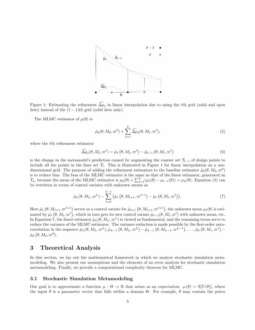
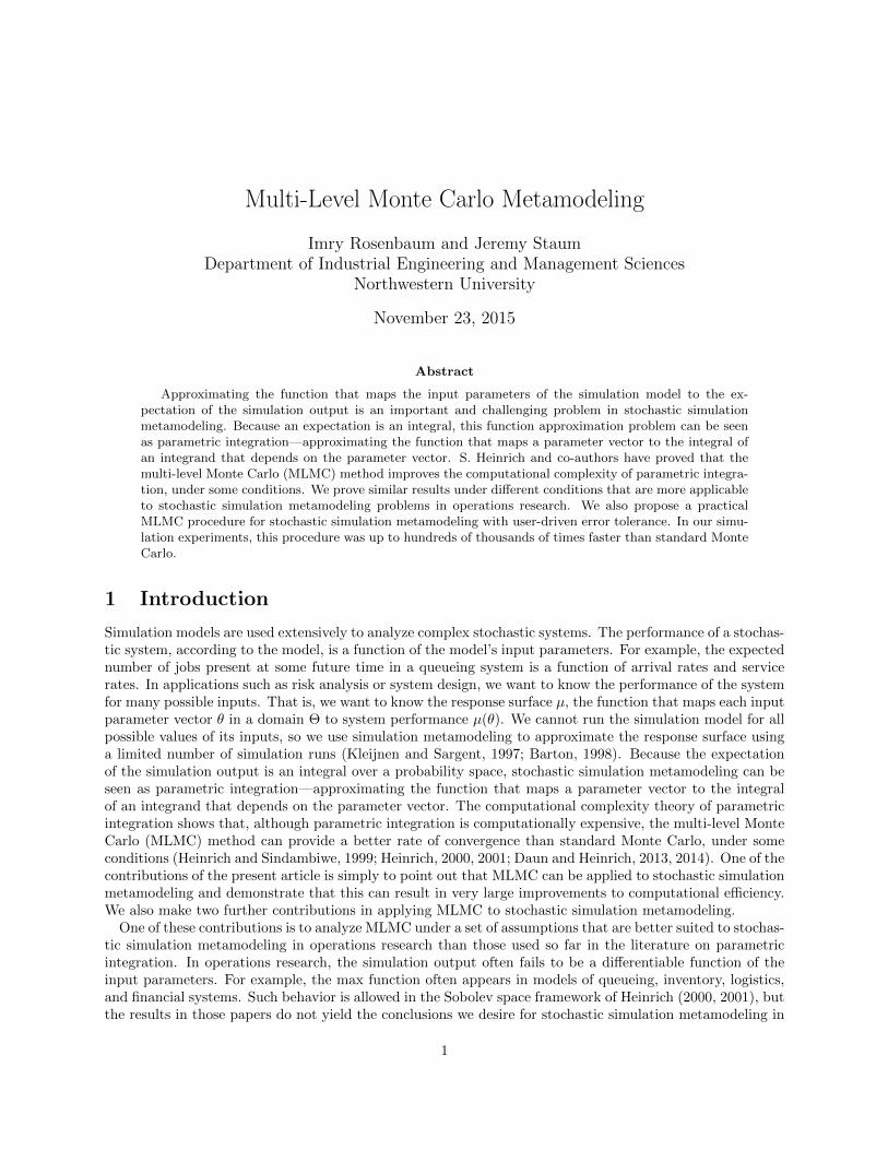
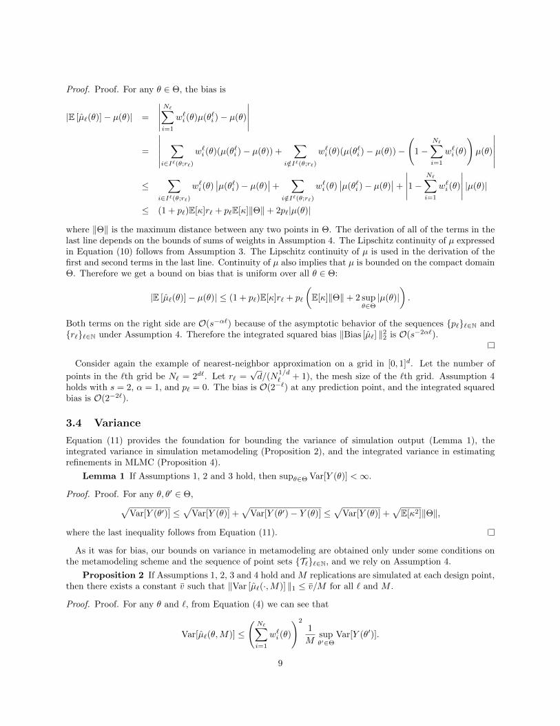
Figure 1: Estimating the refinement ∆µ` in linear interpolation due to using the `th grid (solid and opendots) instead of the (`− 1)th grid (solid dots only).

The MLMC estimator of µ(θ) is

µ0(θ,M0, $0) +

L∑`=1

∆µ`(θ,M`, $`), (5)

where the `th refinement estimator

∆µ`(θ,M`, $`) = µ`

(θ,M`, $

`)− µ`−1

(θ,M`, $

`)

(6)

is the change in the metamodel’s prediction caused by augmenting the coarser set T`−1 of design points toinclude all the points in the finer set T`. This is illustrated in Figure 1 for linear interpolation on a one-dimensional grid. The purpose of adding the refinement estimators to the baseline estimator µ0(θ,M0, $

0)is to reduce bias. The bias of the MLMC estimator is the same as that of the finest estimator, generated onTL, because the mean of the MLMC estimator is µ0(θ) +

∑L`=1(µ`(θ)− µ`−1(θ)) = µL(θ). Equation (5) can

be rewritten in terms of control variates with unknown means as

µL(θ,ML, $L)−

L−1∑`=0

(µ`(θ,M`+1, $

`+1)− µ`

(θ,M`, $

`)). (7)

Here µ`(θ,M`+1, $

`+1)

serves as a control variate for µ`+1

(θ,M`+1, $

`+1), the unknown mean µ`(θ) is esti-

mated by µ`(θ,M`, $

`), which in turn gets its own control variate µ`−1(θ,M`, $

`) with unknown mean, etc.In Equation 7, the finest estimator µL(θ,ML, $

L) is viewed as fundamental, and the remaining terms serve toreduce the variance of the MLMC estimator. The variance reduction is made possible by the first-order auto-correlation in the sequence µL(θ,ML, $

L), µL−1

(θ,ML, $

L)− µL−1

(θ,ML−1, $

L−1), . . . , µ0

(θ,M1, $

1)−

µ0

(θ,M0, $

0).

3 Theoretical Analysis

In this section, we lay out the mathematical framework in which we analyze stochastic simulation meta-modeling. We also present our assumptions and the elements of an error analysis for stochastic simulationmetamodeling. Finally, we provide a computational complexity theorem for MLMC.

3.1 Stochastic Simulation Metamodeling

Our goal is to approximate a function µ : Θ → R that arises as an expectation: µ (θ) = E[Y (θ)], wherethe input θ is a parameter vector that falls within a domain Θ. For example, θ may contain the prices

5

that we set for each of the products our company sells, Y (θ) may be our profit in selling the products atthese prices, and then µ(θ) would be the expected profit. As another example, θ may contain the priceand volatility of a stock and the strike price of an Asian option on the stock, Y (θ) may be the discountedpayoff of an Asian option on such a stock and with such a strike price, and then µ(θ) would be the presentvalue of the Asian option. These examples are discussed in detail in Section 5. In stochastic simulationmetamodeling, we approximate the response surface µ by a metamodel µ. The metamodel is built afterrunning a simulation experiment in which the simulation is run at design points θ1, . . . , θN . At each designpoint θi, we expend computational effort Mi. We assume that Mi is a number of independent replications,each yielding a realization of Y (θ). MLMC is also potentially applicable to steady-state simulations in whichthe computational effort Mi represents run length. Because the variance and bias of the simulation outputbehave differently as computational effort increases in steady-state simulation, we leave this topic for futureresearch.

Our error criterion for assessing the quality of a stochastic simulation metamodeling procedure is meanintegrated squared error:

MISE = E[‖µ− µ‖22

]= E

[∫Θ

(µ(θ)− µ(θ))2

dθ

]=

∫Θ

E[(µ(θ)− µ(θ))

2]

dθ

=

∫Θ

Var [µ(θ)] dθ +

∫Θ

(E [µ(θ)]− µ(θ))2

dθ = ‖Var [µ] ‖1 + ‖Bias [µ] ‖22. (8)

MISE equals integrated mean squared error because the order of integration over Θ and expectation can beinterchanged by Tonelli’s theorem.

To control the MISE of µ, we need to control bias and variance across the domain Θ. To do this, we relyon Assumption 1 about the domain, Assumptions 2 and 3 about the behavior of the simulation output Y (θ)as a function of the input θ, and Assumption 4 about the metamodeling scheme.

Assumption 1 The parameter domain Θ is a compact subset of Rd for some d ∈ N.

3.2 Simulation Output

To formulate our next assumptions, we describe the simulation output Y as a random field. That is, thesimulation output is a measurable function Y : Θ×Ω→ R, where (Ω,F ,P) is a probability space; Lebesguemeasure is the measure on Θ. For any input θ ∈ Θ, the simulation output is a random variable denotedY (θ). The response surface µ is the mean function of the random field: µ(θ) = E[Y (θ)] =

∫Y (θ, ω) dP(ω).

For Monte Carlo, we want finite variance.

Assumption 2 For each θ ∈ Θ, the variance of the simulation output Y (θ) is finite.

Assumption 3 is that the simulation output Y is almost surely Lipschitz continuous, and the coefficient ofLipschitz continuity has finite second moment. The same assumption has also been used to analyze infinites-imal perturbation analysis (also called “pathwise”) Monte Carlo estimators of the gradient of the responsesurface. For example, Glasserman (2004, § 7.2) uses some assumptions, on a more detailed framework inwhich the simulation output Y (θ) arises as a function of underlying random variates generated by the sim-ulation, that are sufficient for Assumption 3 to hold. Using those assumptions, he derives results similar toEquations (10) and (11) below.

Assumption 3 There exists a random variable κ such that E[κ2] is finite and

|Y (θ1, ω)− Y (θ2, ω)| ≤ κ (ω) ‖θ1 − θ2‖ , for all θ1, θ2 ∈ Θ

holds almost surely.

For example, consider simulation output that is exponentially distributed with mean θ ∈ Θ = [0, θmax].This can be described as a random field Y given by Y (θ, ω) = −θ(lnω) for ω ∈ Ω = (0, 1), with theprobability measure P being uniform on Ω. Assumption 3 holds with coefficient κ(ω) = − ln(ω), which hasE[κ2] = 2.

6

We identify a scenario ω ∈ Ω with a sequence of random numbers used in simulation. The function Y (·, ω)is a realization of the random field Y and describes how the simulation output changes as a function ofthe input θ while the random numbers used in the simulation stay the same. In MLMC, it is essentialto use common random numbers in running the simulation with different inputs (Remark 2). The samerandom number stream is used to run the simulation at multiple design points, and it contains independentsubstreams, which are used to generate independent replications of the simulation (L’Ecuyer et al. 2002).Our notation is that the random number stream $ =

ωjj∈N, where the substream ωj generates the jth

replication. The average simulation output from M independent replications run with input θ and randomnumber stream $ is

Y (θ,M,$) =1

M

M∑j=1

Y(θ, ωj

). (9)

We need to consider different random number streams $0, $1, . . . because distinct levels in MLMC aresimulated independently, i.e., with different random number streams. Equation (9) shows that the averagesimulation output forms a random field Y : Θ×N×Ω∞ → R. That is, for any input θ ∈ Θ and positive numberM of replications, Y (θ,M) is a random variable; for any random number stream $ ∈ Ω∞, the functionY (·, ·, $) describes how the average simulation output would change if we changed the input and the numberof replications while using the same random number stream. To make the substreams independent, theprobability space built on Ω∞ involves product measure and the σ-field generated by the set of all cylinders,as is standard (Billingsley, 1995, §2).

Two crucial inequalities follow from Assumption 3. In Section 3.3, we use the Lipschitz continuity of theresponse surface,

|µ(θ + h)− µ(θ)| = |E [Y (θ + h)]− E [Y (θ)]| ≤ E [|Y (θ + h)− Y (θ)|] ≤ E [κ] ‖h‖, (10)

to bound the bias in metamodeling. The bound on the variance of the change in simulation output betweennearby points,

Var [Y (θ + h)− Y (θ)] ≤ E[(Y (θ + h)− Y (θ))

2]

= E[κ2]‖h‖2, (11)

yields a bound on the variance in metamodeling in Section 3.4.

3.3 Bias

Equation (10) can support a bound on the bias in metamodeling. The bias in metamodeling depends onthe metamodeling scheme and the set of design points θ1, . . . , θN at which the simulation is run. A keyfeature of the experiment design is the mesh size of the set of design points,

∆ = maxθ∈Θ

mini=1,...,N

‖θi − θ‖. (12)

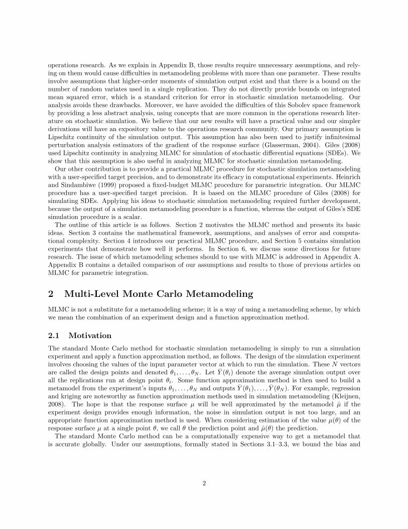
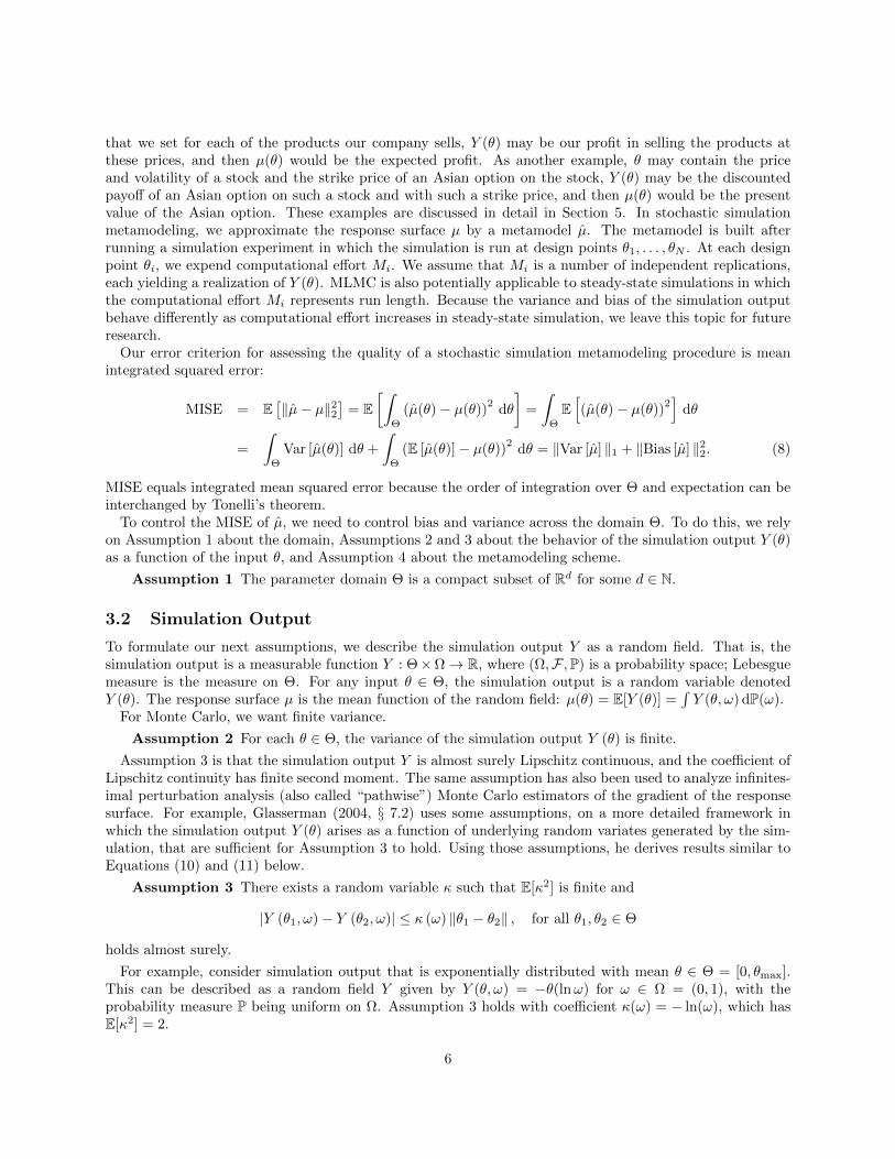
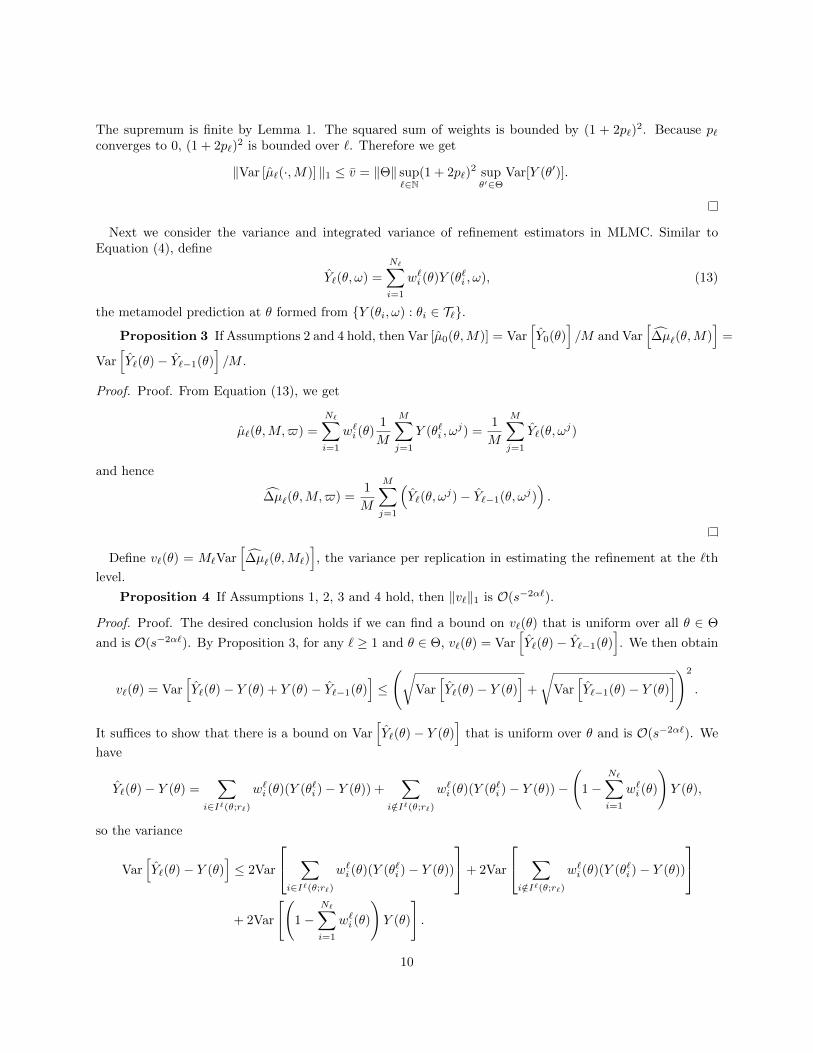
First, let us consider a very simple metamodeling scheme and experiment design: nearest neighbor approxi-mation on a grid. The prediction of the value of the response surface at the prediction point θ is the simulationoutput observed at the design point nearest to θ, i.e., µ (θ) = Y (θi(θ)), where i(θ) = arg mini=1,...,N ‖θi− θ‖.Figure 2 illustrates this metamodeling scheme in an example where the simulation output Y (θ) is an ex-ponential random variable with intensity θ. The bias in this metamodeling scheme is µ(θi(θ)) − µ(θ). Toapply Equation (10), we need to bound the distance from the prediction point to the nearest design point.This is determined by the experiment design. Let Θ, the domain in which the prediction point can belocated, be the hypercube [0, 1]d. Let the experiment design be a grid of N = kd points, each of the form(i1/(k+1), . . . , id/(k+1)), where each i1, . . . , id is an integer between 1 and k. The mesh size of the grid withN points is ∆(N) =

√d/(k + 1) < d1/2N−1/d. From Equation (10), it follows that the bias E[µ(θ)] − µ(θ)

of nearest neighbor approximation with this grid design is bounded by E [κ] d1/2N−1/d, uniformly for allθ ∈ [0, 1]d.

7

Figure 2: Nearest neighbor approximation, where the parameter θ is the intensity of an exponential randomvariable.

For the more general analysis of the way in which the bias in metamodeling depends on the experimentdesign and metamodeling scheme, an asymptotic analysis suffices to support the computational complexityanalysis in Section 3.5. Consider a sequence of experiment designs indexed by `, in which the number ofdesign points N` → ∞. The notation for the point set in the `th experiment design is θ`1, . . . , θ

`N`

. Theexperiment design also includes the number of replications to simulate at each design point, but this is notessential to address while analyzing bias. Let µ` represent the metamodel built from the `th experiment. Asa general matter, what we need is to show that Equation (10) supports a conclusion that ‖Bias [µ`] ‖22, theintegrated squared bias term in Equation (8), is O(s−2α`) for some constants s and α.

The following assumption provides one way of doing that. It expresses the idea that the metamodel’sprediction is a weighted sum that places most of the weight on design points near the prediction point, ifthere are many design points.

Assumption 4 For each θ ∈ Θ and `, Equation (4) holds, and each weight w`i (θ) on the simulationoutput from design point θ`i in predicting at θ in the `th experiment design is a non-negative constant,determined by the experiment design and θ. Define I`(θ; r) = i : ‖θ − θ`i‖ ≤ r, the set of design pointsin the `th experiment design that are within distance r of θ. There exist constants s > 1 and α > 0 andsequences p``∈N and r``∈N such that p` and r` are O(s−α`), and for all θ ∈ Θ,

∑i/∈I`(θ;r`)

w`i (θ) ≤ p` and

∣∣∣∣∣∣1−∑

i∈I`(θ;r`)

w`i (θ)

∣∣∣∣∣∣ ≤ p`.That is, little weight is placed on design points that are far from the prediction point, and the total weight

placed on design points that are near the prediction point nearly equals one. Appendix A.1 provides examplesof metamodeling schemes that satisfy Assumption 4, including grids with piecewise linear interpolation, k-nearest-neighbor approximation, Shepard’s method, or kernel smoothing. A scheme that uses experimentdesigns other than grids, such as low-discrepancy sequences (Asmussen and Glynn, 2007), can also satisfyAssumption 4, if the mesh size converges to zero. A function approximation method that does not fitAssumption 4 is linear regression of the simulation outputs Y (θ`1), . . . , Y (θ`N`

) on the inputs θ`1, . . . , θ`N`

.Linear regression puts large amounts of weight on design points far from the prediction point and generatesnegative weights.

Proposition 1 If Assumptions 1, 3 and 4 hold, then ‖Bias [µ`] ‖22 is O(s−2α`).

8

Proof. Proof. For any θ ∈ Θ, the bias is

|E [µ`(θ)]− µ(θ)| =

∣∣∣∣∣N∑i=1

w`i (θ)µ(θ`i )− µ(θ)

∣∣∣∣∣=

∣∣∣∣∣∣∑

i∈I`(θ;r`)

w`i (θ)(µ(θ`i )− µ(θ)) +∑

i/∈I`(θ;r`)

w`i (θ)(µ(θ`i )− µ(θ))−

(1−

N∑i=1

w`i (θ)

)µ(θ)

∣∣∣∣∣∣≤

∑i∈I`(θ;r`)

w`i (θ)∣∣µ(θ`i )− µ(θ)

∣∣+∑

i/∈I`(θ;r`)

w`i (θ)∣∣µ(θ`i )− µ(θ)

∣∣+

∣∣∣∣∣1−N∑i=1

w`i (θ)

∣∣∣∣∣ |µ(θ)|

≤ (1 + p`)E[κ]r` + p`E[κ]‖Θ‖+ 2p`|µ(θ)|

where ‖Θ‖ is the maximum distance between any two points in Θ. The derivation of all of the terms in thelast line depends on the bounds of sums of weights in Assumption 4. The Lipschitz continuity of µ expressedin Equation (10) follows from Assumption 3. The Lipschitz continuity of µ is used in the derivation of thefirst and second terms in the last line. Continuity of µ also implies that µ is bounded on the compact domainΘ. Therefore we get a bound on bias that is uniform over all θ ∈ Θ:

|E [µ`(θ)]− µ(θ)| ≤ (1 + p`)E[κ]r` + p`

(E[κ]‖Θ‖+ 2 sup

θ∈Θ|µ(θ)|

).

Both terms on the right side are O(s−α`) because of the asymptotic behavior of the sequences p``∈N andr``∈N under Assumption 4. Therefore the integrated squared bias ‖Bias [µ`] ‖22 is O(s−2α`).

Consider again the example of nearest-neighbor approximation on a grid in [0, 1]d. Let the number of

points in the `th grid be N` = 2d`. Let r` =√d/(N

1/d` + 1), the mesh size of the `th grid. Assumption 4

holds with s = 2, α = 1, and p` = 0. The bias is O(2−`) at any prediction point, and the integrated squaredbias is O(2−2`).

3.4 Variance

Equation (11) provides the foundation for bounding the variance of simulation output (Lemma 1), theintegrated variance in simulation metamodeling (Proposition 2), and the integrated variance in estimatingrefinements in MLMC (Proposition 4).

Lemma 1 If Assumptions 1, 2 and 3 hold, then supθ∈Θ Var[Y (θ)] <∞.

Proof. Proof. For any θ, θ′ ∈ Θ,√Var[Y (θ′)] ≤

√Var[Y (θ)] +

√Var[Y (θ′)− Y (θ)] ≤

√Var[Y (θ)] +

√E[κ2]‖Θ‖,

where the last inequality follows from Equation (11).

As it was for bias, our bounds on variance in metamodeling are obtained only under some conditions onthe metamodeling scheme and the sequence of point sets T``∈N, and we rely on Assumption 4.

Proposition 2 If Assumptions 1, 2, 3 and 4 hold and M replications are simulated at each design point,then there exists a constant v such that ‖Var [µ`(·,M)] ‖1 ≤ v/M for all ` and M .

Proof. Proof. For any θ and `, from Equation (4) we can see that

Var[µ`(θ,M)] ≤

(N∑i=1

w`i (θ)

)2

1

Msupθ′∈Θ

Var[Y (θ′)].

9

The supremum is finite by Lemma 1. The squared sum of weights is bounded by (1 + 2p`)2. Because p`

converges to 0, (1 + 2p`)2 is bounded over `. Therefore we get

‖Var [µ`(·,M)] ‖1 ≤ v = ‖Θ‖ sup`∈N

(1 + 2p`)2 supθ′∈Θ

Var[Y (θ′)].

Next we consider the variance and integrated variance of refinement estimators in MLMC. Similar toEquation (4), define

Y`(θ, ω) =

N∑i=1

w`i (θ)Y (θ`i , ω), (13)

the metamodel prediction at θ formed from Y (θi, ω) : θi ∈ T`.

Proposition 3 If Assumptions 2 and 4 hold, then Var [µ0(θ,M)] = Var[Y0(θ)

]/M and Var

[∆µ`(θ,M)

]=

Var[Y`(θ)− Y`−1(θ)

]/M .

Proof. Proof. From Equation (13), we get

µ`(θ,M,$) =

N∑i=1

w`i (θ)1

M

M∑j=1

Y (θ`i , ωj) =

1

M

M∑j=1

Y`(θ, ωj)

and hence

∆µ`(θ,M,$) =1

M

M∑j=1

(Y`(θ, ω

j)− Y`−1(θ, ωj)).

Define v`(θ) = M`Var[∆µ`(θ,M`)

], the variance per replication in estimating the refinement at the `th

level.

Proposition 4 If Assumptions 1, 2, 3 and 4 hold, then ‖v`‖1 is O(s−2α`).

Proof. Proof. The desired conclusion holds if we can find a bound on v`(θ) that is uniform over all θ ∈ Θ

and is O(s−2α`). By Proposition 3, for any ` ≥ 1 and θ ∈ Θ, v`(θ) = Var[Y`(θ)− Y`−1(θ)

]. We then obtain

v`(θ) = Var[Y`(θ)− Y (θ) + Y (θ)− Y`−1(θ)

]≤

(√Var

[Y`(θ)− Y (θ)

]+

√Var

[Y`−1(θ)− Y (θ)

])2

.

It suffices to show that there is a bound on Var[Y`(θ)− Y (θ)

]that is uniform over θ and is O(s−2α`). We

have

Y`(θ)− Y (θ) =∑

i∈I`(θ;r`)

w`i (θ)(Y (θ`i )− Y (θ)) +∑

i/∈I`(θ;r`)

w`i (θ)(Y (θ`i )− Y (θ))−

(1−

N∑i=1

w`i (θ)

)Y (θ),

so the variance

Var[Y`(θ)− Y (θ)

]≤ 2Var

∑i∈I`(θ;r`)

w`i (θ)(Y (θ`i )− Y (θ))

+ 2Var

∑i/∈I`(θ;r`)

w`i (θ)(Y (θ`i )− Y (θ))

+ 2Var

[(1−

N∑i=1

w`i (θ)

)Y (θ)

].

10

Thus, it suffices to exhibit bounds on the variances of each of these three terms that are uniform in θ andare O(s−2α`). Let us call these three variances

1. the variance due to nearby design points,

2. the variance due to distant design points, and

3. the variance due to weights’ failure to sum to one.

Because of Assumption 3, Equation (11) holds. Assumption 4 provides bounds on the sums of weights.Using these facts, we get bounds on each of these three variances that are uniform in θ:

1. The variance due to nearby design points is bounded by (1+p`)E[κ2]r2` . This is where it is essential that

a common random number stream $` is used to simulate at all design points in the `th level. Becauseof that, we can use Lipschitz continuity to bound |Y (θ`i , ω

j)− Y (θ, ωj)| ≤ κ(ωj)|θ`i − θ|; Equation (11)expresses a corresponding bound on variance.

2. The variance due to distant design points is bounded by p2`E[κ2]‖Θ‖2, where ‖Θ‖ is the maximum

distance between any two points in Θ.

3. The variance due to weights’ failure to sum to one is bounded by 4p2` supθ∈Θ Var[Y (θ)]. The supremum

is finite by Lemma 1.

The bounds are all O(s−2α`) due to the asymptotic behavior of the sequences p``∈N and r``∈N underAssumption 4.

3.5 Computational Complexity

In our setting, MLMC is asymptotically more computationally efficient than standard Monte Carlo in reduc-ing MISE, defined in Equation (8). Theorem 1 gives bounds for the computational complexity of standardMonte Carlo and MLMC under the following conditions:

1. The integrated squared bias in metamodeling with the `th experiment design ‖Bias [µ`] ‖22 ≤ (bs−α`)2.

2. The integrated variance in metamodeling ‖Var [µ`(·,M)] ‖1 ≤ vM−1 for all ` and M .

3. The integrated variance per replication in estimating the refinement at the `th level ‖v`‖1 ≤ σ2s−2α`.

4. The number N` of points in the set T` ≤ csγ`.

Under such conditions, similar but more general theorems about MLMC hold, for other problems such assimulation of SDEs as well as parametric integration (Giles, 2013, 2015).

The specifics of stochastic simulation metamodeling enter in two ways. One is in Propositions 1-4, whichshowed that Conditions 1-3 follow from Assumptions 1-4. The other would be in showing that a specificmetamodeling scheme, in which the experiment design satisfies Condition 4 with given s and γ, satisfiesAssumption 4 for a certain value of α. For example, this was done at the end of Section 3.3 for nearest-neighbor approximation on a grid. Theorem 1 is of general use in proving the benefit of MLMC even whennot all of Assumptions 1-4 hold. For example, Theorem 1 may be applied to a metamodeling scheme thatdoes not satisfy Assumption 4 if it can be shown directly that Conditions 1-4 hold.

In the following theorem, we see that computational complexity does not depend on s at all, or on therates α and γ separately, but only on the ratio φ = γ/2α. As we will see in the next section, the factor sγ

for growth in the number of points matters in practice for our MLMC procedure. However, the ratio φ is allthat matters for computational complexity in an asymptotic sense.

Theorem 1 Under Conditions 1–4, the total number of replications that must be simulated to attaina MISE less than ε2 is O(ε−2(1+φ)) for standard Monte Carlo, whereas for MLMC it is

11

• O(ε−2) if φ < 1,

• O((ε−1(log ε−1))2) if φ = 1, or

• O(ε−2φ) if φ > 1.

Proof. Proof. For standard Monte Carlo with point set TL andM replications per design point, the integratedsquared bias ‖Bias [µL] ‖22 ≤ b2s−2αL, and the integrated variance ‖Var [µL(·,M)] ‖1 ≤ vM−1. Take M =2vε−2 and L = (logs(

√2bε−1))/α. This guarantees MISE ≤ ε2. We have NL ≤ csγL, which is O(ε−γ/α).

The computational cost MNL is O(ε−(2+γ/α)).For MLMC, the proof is the same as the proof of Theorem 1 of Cliffe et al. (2011) or Giles (2013). There

is a difference in the setting: the random output of our simulation metamodeling procedure is a function andwe are concerned with its MISE, whereas Giles deals with the MSE of random scalar output. This differenceis immaterial once we have formulated conditions on integrated squared bias and integrated variance thatfit into the framework of conditions that Giles imposes on bias and variance. The other difference is that wehave set Giles’s rate β for the decay of refinement estimators’ variance equal to 2α, because of the effect ofour Assumption 3 through Equation (11) and Proposition 4.

Theorem 1 can be interpreted as saying that stochastic simulation metamodeling may be hard, if φ > 1,or secretly easy, if φ < 1. “Easy” means that the computational cost to attain MISE of ε2 is O(ε−2), whichis the usual computational complexity of Monte Carlo estimation of the expectation of a random variable.“Hard” means that the computational cost to attain MISE of ε2 is not O(ε−2), but grows more rapidly asε→ 0. Although stochastic simulation metamodeling is always hard if you use standard Monte Carlo, it maybe easy if you use MLMC. It is easy with MLMC if φ < 1, or roughly speaking, if doubling the number ofdesign points causes the squared bias and refinement variance to shrink by a factor of more than 2. If φ > 1,then stochastic simulation metamodeling is hard even with MLMC, but the computational complexity isreduced by a factor of ε−2 compared to standard Monte Carlo.

Remark 3 It is not obvious that it is meaningful to compare O(ε−2(1+φ)) and O(ε−2φ) in this way;Theorem 1 merely describes the asymptotic behavior of upper bounds on computational cost. Thereexist stochastic simulation metamodeling problems for which the bounds are not tight: for example, if thesimulation output Y (θ) is linear in the parameter θ, then piecewise linear interpolation on a grid has nobias. Information-based complexity theory can clarify such situations by showing that the bounds are tightfor the worst-case random field Y among a relevant set of random fields. Such a result is given by Heinrichand Sindambiwe (1999).

For the purpose of illustrating how the dimension d of the domain Θ, the function approximation method,and the sequence of point sets T``∈N combine to tell us what α and γ (and therefore φ = γ/2α) should be,let us reconsider a previous example. The example is nearest-neighbor approximation on a grid in Θ = [0, 1]d,

with the `th grid T` having N` = 2d` points and mesh size√d/(N

1/d` + 1). This gives us s = 2 and γ = d.

We showed before how Assumption 4 holds and implies that α = 1. Therefore φ = d/2. Higher dimensiond can make stochastic simulation metamodeling harder. In the one-dimensional case, the computationalcomplexity is O(ε−3) for standard Monte Carlo and O(ε−2) for MLMC. If d > 2, then the computationalcomplexity is O(ε−(d+2)) for standard Monte Carlo and O(ε−d) for MLMC.

4 A Practical Procedure

Theorem 1 describes the computational complexity of attaining MISE less than a target ε2 using MLMCwithout specifying how to attain it. Giles (2008) and Cliffe et al. (2011) analyze the optimal number L oflevels and number M` of replications to use at each level, but these quantities depend on unknowns such asthe bias and refinement variance at each level. Here we present a practical MLMC procedure for attaining thetarget MISE of ε2. We closely follow the procedure of Giles (2008), modifying it because it deals with Monte

12

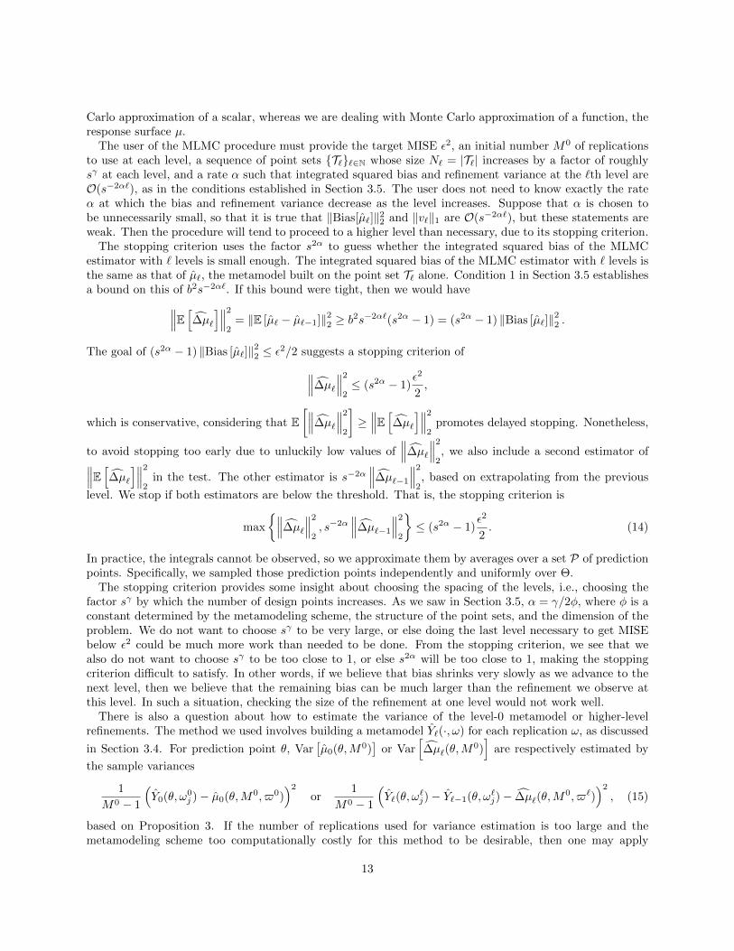
Carlo approximation of a scalar, whereas we are dealing with Monte Carlo approximation of a function, theresponse surface µ.

The user of the MLMC procedure must provide the target MISE ε2, an initial number M0 of replicationsto use at each level, a sequence of point sets T``∈N whose size N` = |T`| increases by a factor of roughlysγ at each level, and a rate α such that integrated squared bias and refinement variance at the `th level areO(s−2α`), as in the conditions established in Section 3.5. The user does not need to know exactly the rateα at which the bias and refinement variance decrease as the level increases. Suppose that α is chosen tobe unnecessarily small, so that it is true that ‖Bias[µ`]‖22 and ‖v`‖1 are O(s−2α`), but these statements areweak. Then the procedure will tend to proceed to a higher level than necessary, due to its stopping criterion.

The stopping criterion uses the factor s2α to guess whether the integrated squared bias of the MLMCestimator with ` levels is small enough. The integrated squared bias of the MLMC estimator with ` levels isthe same as that of µ`, the metamodel built on the point set T` alone. Condition 1 in Section 3.5 establishesa bound on this of b2s−2α`. If this bound were tight, then we would have∥∥∥E [∆µ`]∥∥∥2

2= ‖E [µ` − µ`−1]‖22 ≥ b

2s−2α`(s2α − 1) = (s2α − 1) ‖Bias [µ`]‖22 .

The goal of (s2α − 1) ‖Bias [µ`]‖22 ≤ ε2/2 suggests a stopping criterion of∥∥∥∆µ`

∥∥∥2

2≤ (s2α − 1)

ε2

2,

which is conservative, considering that E[∥∥∥∆µ`

∥∥∥2

2

]≥∥∥∥E [∆µ`]∥∥∥2

2promotes delayed stopping. Nonetheless,

to avoid stopping too early due to unluckily low values of∥∥∥∆µ`

∥∥∥2

2, we also include a second estimator of∥∥∥E [∆µ`]∥∥∥2

2in the test. The other estimator is s−2α

∥∥∥∆µ`−1

∥∥∥2

2, based on extrapolating from the previous

level. We stop if both estimators are below the threshold. That is, the stopping criterion is

max

∥∥∥∆µ`

∥∥∥2

2, s−2α

∥∥∥∆µ`−1

∥∥∥2

2

≤ (s2α − 1)

ε2

2. (14)

In practice, the integrals cannot be observed, so we approximate them by averages over a set P of predictionpoints. Specifically, we sampled those prediction points independently and uniformly over Θ.

The stopping criterion provides some insight about choosing the spacing of the levels, i.e., choosing thefactor sγ by which the number of design points increases. As we saw in Section 3.5, α = γ/2φ, where φ is aconstant determined by the metamodeling scheme, the structure of the point sets, and the dimension of theproblem. We do not want to choose sγ to be very large, or else doing the last level necessary to get MISEbelow ε2 could be much more work than needed to be done. From the stopping criterion, we see that wealso do not want to choose sγ to be too close to 1, or else s2α will be too close to 1, making the stoppingcriterion difficult to satisfy. In other words, if we believe that bias shrinks very slowly as we advance to thenext level, then we believe that the remaining bias can be much larger than the refinement we observe atthis level. In such a situation, checking the size of the refinement at one level would not work well.

There is also a question about how to estimate the variance of the level-0 metamodel or higher-levelrefinements. The method we used involves building a metamodel Y`(·, ω) for each replication ω, as discussed

in Section 3.4. For prediction point θ, Var[µ0(θ,M0)

]or Var

[∆µ`(θ,M

0)]

are respectively estimated by

the sample variances

1

M0 − 1

(Y0(θ, ω0

j )− µ0(θ,M0, $0))2

or1

M0 − 1

(Y`(θ, ω

`j)− Y`−1(θ, ω`j)− ∆µ`(θ,M

0, $`))2

, (15)

based on Proposition 3. If the number of replications used for variance estimation is too large and themetamodeling scheme too computationally costly for this method to be desirable, then one may apply

13

sectioning (Asmussen and Glynn, 2007, § 3.5) so that fewer metamodels need to be built. Other metamodelingschemes, such as stochastic kriging, provide their own variance estimates for a prediction µ`(θ) at thesame time as they make that prediction. In this case, those variance estimates could be used instead ofEquation (15).

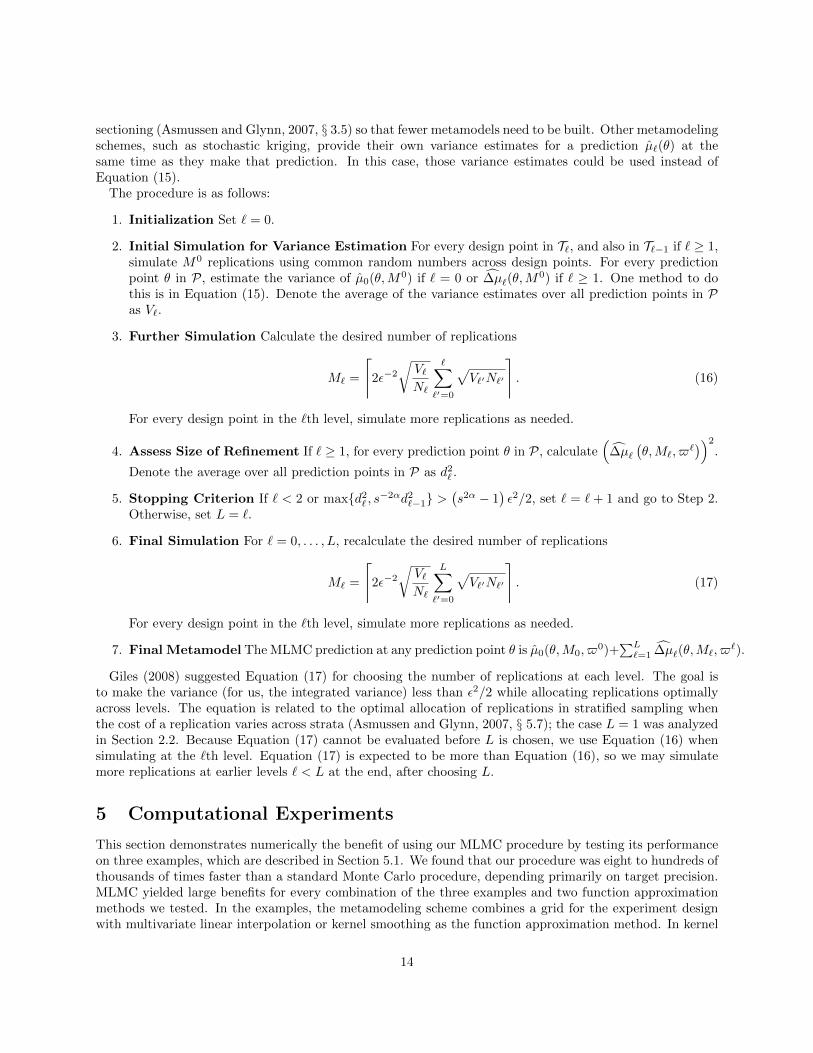
The procedure is as follows:

1. Initialization Set ` = 0.

2. Initial Simulation for Variance Estimation For every design point in T`, and also in T`−1 if ` ≥ 1,simulate M0 replications using common random numbers across design points. For every predictionpoint θ in P, estimate the variance of µ0(θ,M0) if ` = 0 or ∆µ`(θ,M

0) if ` ≥ 1. One method to dothis is in Equation (15). Denote the average of the variance estimates over all prediction points in Pas V`.

3. Further Simulation Calculate the desired number of replications

M` =

⌈2ε−2

√V`N`

∑`′=0

√V`′N`′

⌉. (16)

For every design point in the `th level, simulate more replications as needed.

4. Assess Size of Refinement If ` ≥ 1, for every prediction point θ in P, calculate(

∆µ`(θ,M`, $

`))2

.

Denote the average over all prediction points in P as d2` .

5. Stopping Criterion If ` < 2 or maxd2` , s−2αd2

`−1 >(s2α − 1

)ε2/2, set ` = `+ 1 and go to Step 2.

Otherwise, set L = `.

6. Final Simulation For ` = 0, . . . , L, recalculate the desired number of replications

M` =

⌈2ε−2

√V`N`

L∑`′=0

√V`′N`′

⌉. (17)

For every design point in the `th level, simulate more replications as needed.

7. Final Metamodel The MLMC prediction at any prediction point θ is µ0(θ,M0, $0)+

∑L`=1 ∆µ`(θ,M`, $

`).

Giles (2008) suggested Equation (17) for choosing the number of replications at each level. The goal isto make the variance (for us, the integrated variance) less than ε2/2 while allocating replications optimallyacross levels. The equation is related to the optimal allocation of replications in stratified sampling whenthe cost of a replication varies across strata (Asmussen and Glynn, 2007, § 5.7); the case L = 1 was analyzedin Section 2.2. Because Equation (17) cannot be evaluated before L is chosen, we use Equation (16) whensimulating at the `th level. Equation (17) is expected to be more than Equation (16), so we may simulatemore replications at earlier levels ` < L at the end, after choosing L.

5 Computational Experiments

This section demonstrates numerically the benefit of using our MLMC procedure by testing its performanceon three examples, which are described in Section 5.1. We found that our procedure was eight to hundreds ofthousands of times faster than a standard Monte Carlo procedure, depending primarily on target precision.MLMC yielded large benefits for every combination of the three examples and two function approximationmethods we tested. In the examples, the metamodeling scheme combines a grid for the experiment designwith multivariate linear interpolation or kernel smoothing as the function approximation method. In kernel

14

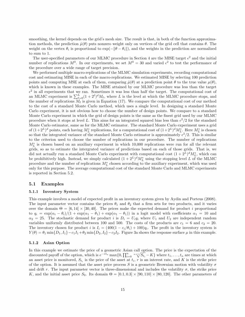
smoothing, the kernel depends on the grid’s mesh size. The result is that, in both of the function approxima-tion methods, the prediction µ(θ) puts nonzero weight only on vertices of the grid cell that contains θ. Theweight on the vertex θi is proportional to exp(−‖θ − θi‖), and the weights in the prediction are normalizedto sum to 1.

The user-specified parameters of our MLMC procedure in Section 4 are the MISE target ε2 and the initialnumber of replications M0. In our experiments, we set M0 = 30 and varied ε2 to test the performance ofthe procedure over a wide range of target precision.

We performed multiple macro-replications of the MLMC simulation experiments, recording computationalcost and estimating MISE in each of the macro-replications. We estimated MISE by selecting 100 predictionpoints and computing MSE at each of them, comparing µ(θ) at a prediction point θ to the true value µ(θ),which is known in these examples. The MISE attained by our MLMC procedure was less than the targetε2 in all experiments that we ran. Sometimes it was less than half the target. The computational cost ofan MLMC experiment is

∑L`=0(1 + 2`)dM`, where L is the level at which the MLMC procedure stops, and

the number of replications M` is given in Equation (17). We compare the computational cost of our methodto the cost of a standard Monte Carlo method, which uses a single level. In designing a standard MonteCarlo experiment, it is not obvious how to choose the number of design points. We compare to a standardMonte Carlo experiment in which the grid of design points is the same as the finest grid used by our MLMCprocedure when it stops at level L. This aims for an integrated squared bias less than ε2/2 for the standardMonte Carlo estimator, same as for the MLMC estimator. The standard Monte Carlo experiment uses a gridof (1+2L)d points, each having M∗L replications, for a computational cost of (1+2L)dM∗L. Here M∗L is chosenso that the integrated variance of the standard Monte Carlo estimator is approximately ε2/2. This is similarto the criterion used to choose the number of replications in our procedure. The number of replicationsM∗L is chosen based on an auxiliary experiment in which 10,000 replications were run for all the relevantgrids, so as to estimate the intergrated variance of predictions based on each of those grids. That is, wedid not actually run a standard Monte Carlo experiment with computational cost (1 + 2L)dM∗L, which canbe prohibitively high. Instead, we simply calculated (1 + 2L)dM∗L using the stopping level L of the MLMCprocedure and the number of replications M∗L chosen according to the auxiliary experiment, which was usedonly for this purpose. The average computational cost of the standard Monte Carlo and MLMC experimentsis reported in Section 5.2.

5.1 Examples

5.1.1 Inventory System

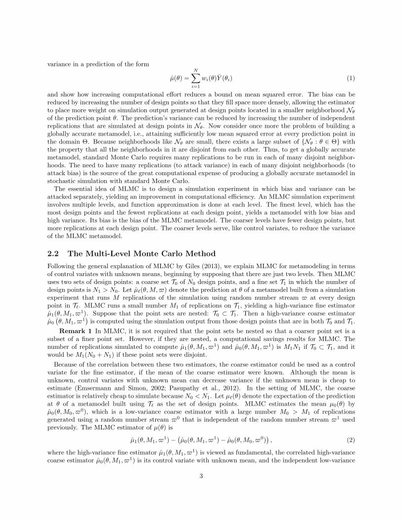
This example involves a model of expected profit in an inventory system given by Aydin and Porteus (2008).The input parameter vector contains the prices θ1 and θ2 that a firm sets for two products, and it variesover the domain Θ = [6, 14] × [30, 40]. The prices make the expected demand for product i proportionalto qi = exp(αi − θi)/(1 + exp(α1 − θ1) + exp(α1 − θ1)) in a logit model with coefficients α1 = 10 andα2 = 25. The stochastic demand for product i is Di = Uiqi where U1 and U2 are independent randomvariables uniformly distributed between 100 and 500. The costs of the products are c1 = 6 and c2 = 20.The inventory chosen for product i is Ii = (400(1 − ci/θi) + 100)qi. The profit in the inventory system isY (θ) = θ1 minD1, I1−c1I1 +θ2 minD2, I2−c2I2. Figure 3a shows the response surface µ in this example.

5.1.2 Asian Option

In this example we estimate the price of a geometric Asian call option. The price is the expectation of thediscounted payoff of the option, which is e−rtn max0,

∏ni=0

n+1√Sti−K where t1, . . . , tn are times at which

an asset price is monitored, Sti is the price of the asset at ti, r is an interest rate, and K is the strike priceof the option. It is assumed that the asset price process S is a geometric Brownian motion with volatility σand drift r. The input parameter vector is three-dimensional and includes the volatility σ, the strike priceK, and the initial asset price S0. Its domain Θ = [0.1, 0.3] × [90, 110] × [80, 120]. The other parameters of

15

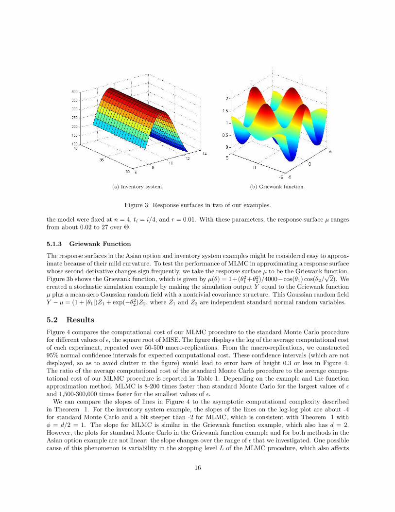
(a) Inventory system. (b) Griewank function.

Figure 3: Response surfaces in two of our examples.

the model were fixed at n = 4, ti = i/4, and r = 0.01. With these parameters, the response surface µ rangesfrom about 0.02 to 27 over Θ.

5.1.3 Griewank Function

The response surfaces in the Asian option and inventory system examples might be considered easy to approx-imate because of their mild curvature. To test the performance of MLMC in approximating a response surfacewhose second derivative changes sign frequently, we take the response surface µ to be the Griewank function.Figure 3b shows the Griewank function, which is given by µ(θ) = 1+(θ2

1 +θ22)/4000−cos(θ1) cos(θ2/

√2). We

created a stochastic simulation example by making the simulation output Y equal to the Griewank functionµ plus a mean-zero Gaussian random field with a nontrivial covariance structure. This Gaussian random fieldY − µ = (1 + |θ1|)Z1 + exp(−θ2

2)Z2, where Z1 and Z2 are independent standard normal random variables.

5.2 Results

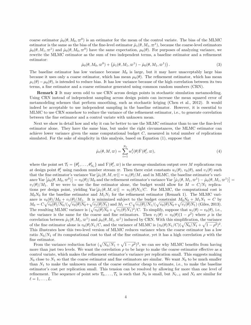
Figure 4 compares the computational cost of our MLMC procedure to the standard Monte Carlo procedurefor different values of ε, the square root of MISE. The figure displays the log of the average computational costof each experiment, repeated over 50-500 macro-replications. From the macro-replications, we constructed95% normal confidence intervals for expected computational cost. These confidence intervals (which are notdisplayed, so as to avoid clutter in the figure) would lead to error bars of height 0.3 or less in Figure 4.The ratio of the average computational cost of the standard Monte Carlo procedure to the average compu-tational cost of our MLMC procedure is reported in Table 1. Depending on the example and the functionapproximation method, MLMC is 8-200 times faster than standard Monte Carlo for the largest values of εand 1,500-300,000 times faster for the smallest values of ε.

We can compare the slopes of lines in Figure 4 to the asymptotic computational complexity describedin Theorem 1. For the inventory system example, the slopes of the lines on the log-log plot are about -4for standard Monte Carlo and a bit steeper than -2 for MLMC, which is consistent with Theorem 1 withφ = d/2 = 1. The slope for MLMC is similar in the Griewank function example, which also has d = 2.However, the plots for standard Monte Carlo in the Griewank function example and for both methods in theAsian option example are not linear: the slope changes over the range of ε that we investigated. One possiblecause of this phenomenon is variability in the stopping level L of the MLMC procedure, which also affects

16

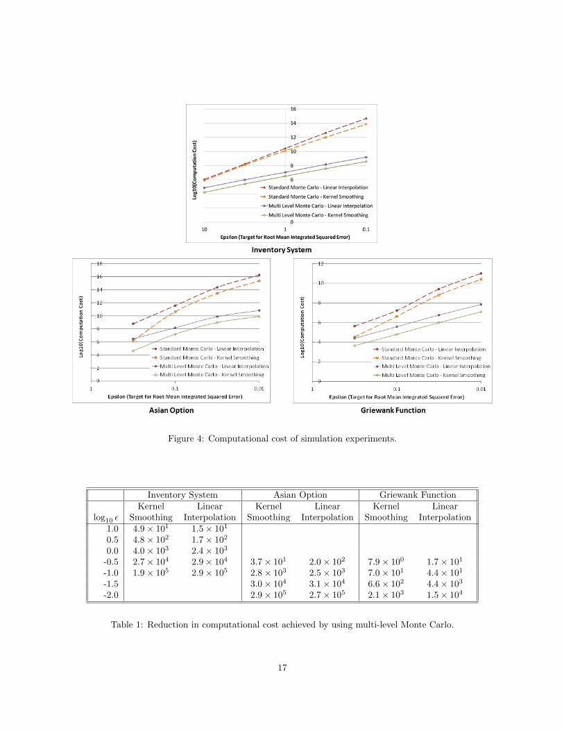
Figure 4: Computational cost of simulation experiments.

Inventory System Asian Option Griewank FunctionKernel Linear Kernel Linear Kernel Linear

log10 ε Smoothing Interpolation Smoothing Interpolation Smoothing Interpolation1.0 4.9× 101 1.5× 101

0.5 4.8× 102 1.7× 102

0.0 4.0× 103 2.4× 103

-0.5 2.7× 104 2.9× 104 3.7× 101 2.0× 102 7.9× 100 1.7× 101

-1.0 1.9× 105 2.9× 105 2.8× 103 2.5× 103 7.0× 101 4.4× 101

-1.5 3.0× 104 3.1× 104 6.6× 102 4.4× 103

-2.0 2.9× 105 2.7× 105 2.1× 103 1.5× 104

Table 1: Reduction in computational cost achieved by using multi-level Monte Carlo.

17

the computational cost of the standard Monte Carlo procedure through the choice of grid. Another possibleexplanation for the difference between the theoretical rates in Theorem 1 and slopes seen in Figure 4 isthat the theorem describes asymptotic growth rates of upper bounds on computational cost. Some valuesof ε in our computational experiments may be too small to see asymptotic behavior, and some functionapproximation methods may perform exceptionally well for some grids and some response surfaces. Forexample, the performance of kernel smoothing is surprisingly good for the largest value of ε for standardMonte Carlo in the Griewank function example and for both standard Monte Carlo and MLMC in the Asianoption example.

6 Future Research

We believe that MLMC is a very valuable tool for stochastic simulation metamodeling and worthy of furtherdevelopment for this application. Here we sketch a few directions for future research in this area.

We provided a simple MLMC procedure for stochastic simulation metamodeling, building on the MLMCprocedure of Giles (2008) for SDE simulation. Recent advances in the design of MLMC procedures forSDE simulation and other applications might be applied to build better MLMC procedures for stochasticsimulation metamodeling. Haji-Ali et al. (2014) explored optimization of the sequence of experiment designs,the stopping criterion for number of levels, and the number of replications. Hoel et al. (2012) developedan adaptive experiment design which, in our setting, might correspond to using a different experimentdesign for each realization of the simulation output, Y (·, ω). Mes et al. (2011) also developed an adaptiveexperiment design featuring multiple levels of coarseness; although their problem was discrete optimizationvia simulation, their work may be relevant to MLMC in stochastic simulation metamodeling.

We showed how MLMC can improve the rate of convergence in stochastic simulation metamodeling whenerror is measured based on the ‖ · ‖2 norm and under conditions including Lipschitz continuity of thesimulation output. Similar results could be derived using different norms and different conditions on thesimulation output or also response surface. We previously derived similar results under the condition ofHolder continuity (Rosenbaum and Staum, 2013), but for operations research applications, it would be muchmore valuable to allow for some discontinuity in the simulation output. We are presently working on thistopic. The ‖ · ‖∞ norm and higher-order smoothness are discussed in the Appendices.

McLeish (2011) provided a general method for eliminating the bias from a Monte Carlo estimator whosebias can be made to converge to zero by increasing computational effort. In the language of MLMC, hismethod involves randomizing the number of replications M` for each level ` in such a way that the numberof levels L is random, M1, . . . ,ML are non-increasing, M` = 0 for ` > L, and E[M`] > 0 for all `. Thismethod can improve the computational complexity of simulating SDEs with time-discretization bias (Rheeand Glynn, 2012, 2013); recently it was also used to approximate expectations taken under the equilibriumdistribution of a positive Harris recurrent Markov chain (Glynn and Rhee, 2014). The same idea should beapplicable to stochastic simulation metamodeling.

Finally, consider simulation metamodeling when a simulation run at a design point θ provides a biasedestimator of µ(θ), such as simulation of SDEs with time-discretization bias or steady-state simulation withinitial-condition bias. Suppose that the bias-elimination technique described in the previous paragraph isapplied to the simulation runs. Then the simulation metamodeling problem is returned to the frameworkconsidered in this article, in which the simulation runs provide unbiased estimators. Alternatively, for somesuch simulation metamodeling problems with biased simulation runs, one might instead try to control twokinds of bias simultaneously: the bias from function approximation, reduced by using many design points,and the bias inherent in simulation runs, reduced by increasing the computational effort per simulation run.Future research may address these questions of experiment design and the effectiveness of such simulationmetamodeling procedures.

18

A Applicability of MLMC

With which metamodeling schemes should MLMC be applied? MLMC improves the computational complex-ity of simulation metamodeling if our assumptions are satisfied. Among them, Assumption 4 is an assumptionabout the metamodeling scheme: the function approximation method and sequence of experiment designs.To satisfy Assumption 4, it is necessary that the function approximation method yield a prediction in theform of Equation (1), and that the sequence of experiment designs have a mesh size, defined in Equation (12),that converges to zero at an appropriate rate. In Appendix A.1, we describe some schemes that satisfy As-sumption 4. Appendix A.2 contains further remarks on function approximation methods that might be usedwith MLMC.

First, we make a general remark about experiment design. For simplicity, we have used grids in ourexamples and computational experiments. However, a grid does not fill high-dimensional space efficiently.In simulation metamodeling, it seems better to use other space-filling experiment designs, such as low-discrepancy point sets (Asmussen and Glynn, 2007) or sparse grids (Barthelmann et al., 2000).

A.1 Some Specific Metamodeling Schemes that Satisfy Assumption 4

Heinrich (2000) mentioned piecewise multivariate linear interpolation as a function approximation methodthat is suitable for MLMC. Consider a d-dimensional grid for which the vector h specifies the width of a gridcell in each of the coordinates; the mesh size is ‖h‖. Let N (θ) be the set of design points neighboring theprediction point θ. If θ is in the interior of a grid cell, then N (θ) is the set of the 2d vertices of this grid cell.Piecewise linear interpolation on a grid can be done with tensor-product piecewise linear B-splines (Hastieet al., 2009), yielding a prediction in the form of Equation (1) with weight

wi(θ) =

d∏j=1

|θj − θij |hj

if θi ∈ N (θ), wi(θ) = 0 if θi /∈ N (θ).

Let h` specify the cell widths in the `th experiment design. If ‖h`‖ is O(s−α`), then Assumption 4 holdswith r` = ‖h`‖ and p` = 0.

Next we consider function approximation methods that work with scattered data, i.e., the experimentdesign need not have a special structure such as a grid. Assume that ∆`, the mesh size of the `th experimentdesign, is O(s−α`).

One simple method is k-nearest-neighbor approximation (Hastie et al., 2009), which puts weight 1/k oneach of the k design points nearest the prediction point and weight 0 on all other design points in Equation (1).Assumption 4 holds with r` = 2k∆` and p` = 0.

As an alternative, let the weight wi(θ) on design point θi depend on the distance ‖θ−θi‖ to the predictionpoint θ. A non-increasing function ψ is used to set the influence ψ(t) given to a design point at distance tfrom the prediction point. The weight for design point θi in Equation (1) is

wi(θ) =ψ(‖θ − θi‖)∑Ni′=1 ψ(‖θ − θi′‖)

.

If ψ is strictly positive, then the prediction is a weighted average involving all of the design points; ifψ(t) = 0 for t exceeding a threshold t, then only nearby design points enter into the weighted average.Shepard’s method (Buhmann, 2003) uses such weights with a function ψ such that ψ(0) = ∞ and ψ(t) isfinite for t > 0. The purpose of this is to ensure µ(θi) = Y (θi), i.e., Shepard’s method is an interpolationmethod. The same formula for weights is used in kernel smoothing (Hastie et al., 2009). If ψ(0) is finite,this causes smoothing, meaning that µ(θi) can depend on simulation output at design points other than θi.Let ψ` be the weighting function used with the `th experiment design. We consider two different cases inwhich Assumption 4 holds for Shepard’s method and kernel smoothing.

1. Suppose that there is a threshold t` > ∆` such that ψ`(t) = 0 for all t > t`, and t` is O(s−α`). ThenAssumption 4 holds with r` = t` and p` = 0.

19

2. Finally, consider a case in which positive weight is given to distant design points. Suppose that thereis a function ψ such that limt→∞ ψ(t) = 0 and a bandwidth h` such that for all t, ψ`(t) = ψ(t/h`).Suppose the mesh size ∆` ≤ c∆s−` and the number N` of points in the `th experiment design satisfiesN` ≤ cNs

d` for some constants c∆ and cN ; this can be achieved by a sequence of grids. Suppose thebandwidth h` = chs

−β` where ch > 0 and β ∈ (0, 1) are constants. Set r` = c∆s−α` for α ∈ (0, β).

This makes r` ≥ ∆`. In the `th experiment design, for any prediction point θ, there is at least onedesign point within distance ∆`, i.e., in I`(θ; ∆`). This design point θi is in I`(θ; r`) and it receivesun-normalized weight ψ`(‖θ−θi‖) ≥ ψ(∆`/h`) ≥ ψ(c∆/ch). Any design point θi′ that is not in I`(θ; r`)receives un-normalized weight ψ`(‖θ − θi′‖) ≤ ψ(r`/h`) ≤ ψ((c∆/ch)s(β−α)`). The total amount ofnormalized weight given to distant design points is

∑i′ /∈I`(θ;r`)

w`i′(θ) =

∑i′ /∈I`(θ;r`) ψ

`(‖θ − θi′‖)∑i′ /∈I`(θ;r`) ψ

`(‖θ − θi′‖) +∑i∈I`(θ;r`) ψ

`(‖θ − θi‖)

≤∑i′ /∈I`(θ;r`) ψ

`(‖θ − θi′‖)∑i∈I`(θ;r`) ψ

`(‖θ − θi‖)≤ N`ψ((c∆/ch)s(β−α)`)

ψ(c∆/ch)= p`,

where this serves to define p`. Suppose that ψ(t) is O(t−(α+d)/(β−α)). Then ψ((c∆/ch)s(β−α)`) isO(s−(α+d)`). Together with N` being O(sd`), this implies that p` is O(s−α`). Thus, Assumption 4holds.

A.2 Function Approximation Methods to Use with MLMC

Before addressing specific methods, we discuss how an approach slightly different from that in this articlecould be helpful in verifying a method’s suitability for MLMC. Theorem 1 is founded on Equation (8), wherewe decomposed MISE into integrated variance plus integrated squared bias. This is similar to the standarddecomposition of MSE into variance plus bias, which Giles (2008) used. A slightly different perspective wastaken by Heinrich, who focused on function approximation methods that are used when the function beingapproximated can be observed without noise. Imagine that we could actually observe µ(θi) at each of thedesign points. Applying the function approximation method described in Equation (1) to these observations,

we would get µ(θ) =∑Ni=1 wi(θ)µ(θi) as the zero-noise prediction of the value of the response surface at the

prediction point θ. Then MISE can be bounded as

E[‖µ(θ)− µ(θ)‖22] ≤ ‖µ(θ)− µ(θ)‖22 + E[‖µ(θ)− µ(θ)‖22], (18)

the sum of the deterministic integrated squared error of approximating the response surface in this scheme,plus the MISE of the noisy metamodel µ(θ) considered as an estimator of the zero-noise metamodel µ(θ). Inthe case of linear prediction as in Equation (1), equality holds and Equation (18) coincides with Equation (8)because E[µ(θ)] = µ(θ). Nonetheless, adopting the perspective of Equation (18) may be advantageous inchecking whether a metamodeling scheme satisfies the conditions for MLMC to improve computationalcomplexity. Instead of trying to analyze the bias of the metamodel given noisy data, one might consult theliterature for error bounds on the deterministic function approximation method. The way to deal with thelast term in Equation (18) is discussed in Appendix B.4.

Consider function approximation methods that fit the form of Equation (1), rewritten as

µ(θ) =

N∑i=1

wi(θ)Y (θi) =

N∑i=1

p∑j=1

Qijϕj(θ)Y (θi) =

p∑j=1

βjϕj(θ), (19)

where ϕ1, . . . , ϕp are basis functions and Q is a matrix such that the weight on the ith design point wi(θ) =∑pj=1Qijϕj(θ) and the coefficient on the jth basis function βj =

∑Ni=1Qij Y (θi). This form applies to

regression, kriging, splines (Hastie et al., 2009), and radial basis functions (Buhmann, 2003), as well as their

20

regularized or smoothing versions. These methods have much in common. Indeed, kriging can be seen as aform of regression, and in some circumstances, the same function approximation can be reached via splines,radial basis functions, or kriging (Myers, 1992).

The phrase “basis functions” indicates that ϕnn∈N forms a basis for a space F of functions; the meta-model µ must be in F . For MLMC to be applicable, there should be a sequence of functions fn in F suchthat the error fn−µ in approximating the response surface µ converges to zero in the desired sense. (In thesetting of this article, it would be that the integrated squared error ‖fn−µ‖22 =

∫Θ

(fn(θ)−µ(θ))2 dθ goes tozero.) For example, quadratic regression is inappropriate as a method to use with MLMC, because we cannotassume that the response surface can be well approximated by a quadratic function of θ. Sobolev spaces seemto be a good choice for F . They are connected with the spline and radial basis function methods for functionapproximation (Fasshauer, 2012). They also accommodate the use of higher-order function approximationmethods to attain better rates of convergence when the function being approximated is smoother.

A limitation of Equation (19) is that it has weights that do not depend on simulation output. In practice,the weights often involve bandwidths, smoothing parameters, or other parameters that are selected using thesimulation output. Addressing that issue might complicate the analysis, but we suspect it that it need not bean obstacle to applying MLMC with these methods even when using a good parameter-selection technique.

Next, consider moving least squares regression (Levin, 1998; Salemi et al., 2012), also called “local regres-sion” (Loader, 1999; Hastie et al., 2009). In this method, Equation (19) applies, except that the coefficients

βj(θ) are allowed to depend on the prediction point θ. This allows moving least squares regression to ap-proximate a larger space of functions than the corresponding form of ordinary regression. For example,continuously differentiable functions are locally linear, and Levin (1998) has a theorem providing the rate ofconvergence for moving least squares linear regression to approximate a continuously differentiable function,with error measured by the ‖ · ‖∞ norm. We conjecture that the same rate would obtain for moving leastsquares linear regression to approximate a Lipschitz-continuous function, with error measured by the ‖ · ‖2norm. For the reason, see Appendix B.3, where we sketch the connection between Lipschitz continuity andHeinrich’s Sobolev space framework.

Finally, neural networks can approximate a large space of functions. The details depend on the architec-ture of the neural network, and the architecture may need to increase in size to allow approximation errorto converge to zero. For example, neural networks can approximate any continuous function on a compact,convex subset of Rd, but the required number of nodes in the network may go to infinity as the approxi-mation error goes to zero. See Kainen et al. (2013) for an overview of results on function approximation byneural networks and associated rates of convergence. Training a neural network can be much more difficultthan computing good coefficients βj in Equation (19). Care should be taken to ensure that the functionapproximation is actually improved by expanding the point set. One might even consider, in Equation (6),using the neural network for µ`−1 as a starting point for building the neural network for µ`.

B Relation to Previous Research

MLMC for parametric integration was analyzed originally by Heinrich and Sindambiwe (1999) and Heinrich(2000, 2001), and recently by Daun and Heinrich (2013, 2014), using different assumptions on the simulationoutput Y : Θ × Ω → R. Among the assumptions of Heinrich and Sindambiwe (1999) and Daun andHeinrich (2013, 2014) is that Y is continuously differentiable on Θ× Ω. Similarly, Y must have continuouspartial derivatives with respect to the parameters in θ for the analysis of Daun and Heinrich (2014) to yielduseful results. As discussed in Section 1, it is common in stochastic simulation metamodeling in operationsresearch for Y to have points of non-differentiability with respect to the parameter θ. This is allowed underthe smoothness assumptions of Heinrich (2000, 2001). However, his assumptions about Θ and Ω, and theintegrability properties of Y on Θ×Ω, create obstacles to the direct application of his results for our purposes.We avoid these difficulties by assuming instead that Θ is compact, as do Heinrich and Sindambiwe (1999) andDaun and Heinrich (2013, 2014). To summarize the position of our work relative to the previous literature:

• Our work has a mixture of some assumptions of Heinrich (2000, 2001), allowing for Y not to be

21

differentiable everywhere with respect to the parameters in θ, and the assumption of Heinrich andSindambiwe (1999) and Daun and Heinrich (2013, 2014) that the domain Θ is compact.

• Our work is more general in that it drops the assumption that Ω is finite-dimensional, which was madein all of the articles mentioned here.

• Our work is less general in neglecting the benefits of higher-order smoothness, e.g., existence of secondderivatives. Whereas we consider only Lipschitz continuity, the previous literature also shows howhigher-order smoothness can improve the computational complexity of MLMC.

In this appendix, we discuss the applicability of the assumptions of Heinrich (2001) in detail, using ournotation rather than his, and explain how his results relate to ours. Lastly, we present a fuller exposition ofHeinrich’s approach to error analysis based on the theory of random fields, and state how it can be used inour setting.

B.1 The Probability Space

Heinrich assumed that the integration in parametric integration is integration over a subset Ω ⊂ Rd2 withrespect to a uniform measure, and approximated integrals of the form

∫ΩY (θ, ω) dω by Monte Carlo sampling

of random variates uniformly distributed on Ω. However, as Heinrich (2001) remarked, it is not necessary tosample uniformly on Ω; importance sampling could be used instead. We believe that it remains within thespirit of Heinrich’s work to observe that, likewise, it is not necessary for the integral to be with respect toa uniform measure in the first place, nor is it necessary for the domain of integration to be a subset of Rd2for some d2. Indeed, d2 does not appear in Heinrich’s computational complexity theorems. Consequently,we have made no assumption about the probability space (Ω,P) in which we have a stochastic model andapproximate expectations by Monte Carlo. We merely assume that this can be done in the usual way, withzero bias and finite variance. In particular, we wish to make it clear that our analysis of MLMC applies tosimulation models in which the number of random variates generated per replication is unbounded (insteadof being bounded by d2).

B.2 The Parameter Domain

Heinrich assumed that the parameter domain Θ ∈ Rd, over which the response surface µ = E[Y ] is to beapproximated, is a bounded open set. Making Θ an open set allows for Y and µ to be unbounded, evenif they are continuous. As an example in operations research, we might think of queueing system behavioron an open set of parameter values for which the system is stable, e.g., in an M/M/1 queue with arrivalrate a and service rate b, taking Θ = (a, b) : 1 < a < b < 2. With an open domain like this, simulationmetamodeling necessarily involves extrapolation. We suppose that in simulation metamodeling in operationsresearch, it is not common to aim for high precision in the predictions from a metamodel outside the rangeof parameter values explored in the experiment design, and where the response surface may be unbounded.Instead, our Assumption 1 is that Θ is a compact set in Rd. Similarly, Heinrich and Sindambiwe (1999) andDaun and Heinrich (2014) assumed that Θ = [0, 1]d.

Equation (10) shows that the response surface µ is Lipschitz continuous. Therefore it is bounded on Θ.Likewise, almost surely, Y (·, ω) is Lipschitz continuous and therefore bounded on Θ. Similarly, if µ is aweighted sum of simulation output, as in our Assumption 4, then µ too is almost surely Lipschitz continuousand therefore bounded on Θ.

Heinrich further assumed that Θ has Lipschitz boundary. This is a standard regularity property to assumefor bounded open subsets of Rd in the theory of Sobolev spaces (Adams, 1975, pp. 66-67), which Heinrichused. The assumption of Lipschitz boundary is not necessary in our simpler setting.

22

B.3 Smoothness and Integrability

Heinrich assumed that for some degree of smoothness r ∈ N and exponent of integrability q ∈ [1,∞]satisfying the Sobolev embedding condition r/d > 1/q, the function Y is in the space W r,0

q (Θ×Ω), a slightlynon-standard Sobolev space to be defined below. See Adams (1975) for the mathematics of Sobolev spaces.

The exponent q governs the norm which is used in quantifying error. For 1 ≤ q < ∞, the norm of theerror is

‖µ− µ‖q =

(∫Θ

|µ(θ)− µ(θ)|q dθ

)1/q

.

For q =∞, ‖µ− µ‖∞ is the greatest lower bound of the set of constants K such that |µ(θ)− µ(θ)| ≤ K foralmost every θ ∈ Θ. Supposing that µ and µ are bounded on Θ (see Section B.2), ‖µ − µ‖∞ is simply themaximum value attained by |µ(θ) − µ(θ)| for any θ ∈ Θ. Thus, q = ∞ is of interest as the worst error ofthe metamodel. Also of interest is q = 2, because ‖µ − µ‖22 is the integrated squared error which goes intoMISE, a standard way to measure quality in stochastic simulation metamodeling. Separate computationalcomplexity theorems cover the cases 1 ≤ q < ∞ and q = ∞, and the computational complexity is worsewhen one wishes to bound ‖µ− µ‖∞ (Heinrich, 2001). We have focused on the case q = 2.

The order of smoothness r relates to how many times the function Y can be weakly differentiated withrespect to parameters in the vector θ ∈ Θ. Weak differentiation is the concept of differentiation used inSobolev spaces. For example, the function f given by f(θ) = max0, θ is not differentiable on [−1, 1], but itis weakly differentiable on [−1, 1]. The functions given by 1θ > 0 and 1θ ≥ 0 are both weak derivativesof f on [−1, 1]. The weak derivative of a function can be thought of as being unique as an equivalence classof all weak derivatives, because the weak derivatives of a single function must be equal almost everywhereand they must equal the ordinary derivative wherever it exists. The weak derivative of f is discontinuous at0, so f is not twice weakly differentiable. With this example in mind, we take r = 1 to be most appropriatefor stochastic simulation metamodeling in operations research, although higher-order smoothness can occur.

To define the Sobolev space W r,0q (Θ × Ω), we must consider weak partial derivatives. Let α represent a

multi-index, a vector of length d+d2 in Heinrich’s setting, such that αi is the number of times to differentiate(weakly) with respect to the ith coordinate. Let |α|θ =

∑di=1 αi be the total number of times to differentiate

with respect to the parameters in θ and |α|ω =∑d2i=d+1 αi be the total number of times to differentiate with

respect to the coordinates of ω; also let |α| = |α|θ + |α|ω. Let DαY represent Y ’s weak partial derivative oforder α; if the partial derivative of order α in the ordinary sense were to exist, it would be written

∂|α|Y

∂θα11 · · · ∂θ

αd

d ∂ωαd+1

1 · · · ∂ωαd+d2

d2

.

The assumption that the function Y is in the space W r,0q (Θ× Ω) means that Y satisfies∫

Θ×Ω

|DαY |q dω dθ <∞

for all α such that 0 ≤ |α|θ ≤ r and |α|ω = 0. To paraphrase Heinrich (2001), this means roughly that withrespect to θ, Y (θ, ω) behaves like a function in the Sobolev space W r

q (Θ), and with respect to ω, it behaveslike a function in the Sobolev space W 0

q (Ω) = Lq(Ω). This gives us a second reason to focus on the caseq = 2: we have no desire to impose an assumption that the simulation output has moments of order higherthan 2.

However, there is an obstacle to applying Heinrich’s results to our desired case of r = 1 and q = 2: theSobolev embedding condition r/d > 1/q fails to hold for dimension d > 1. This turns out to be irrelevantin our setting. The Sobolev embedding condition is used to ensure that functions in a Sobolev spaceW rq on a d-dimensional domain are continuous. Heinrich (2008) addresses the case in which the Sobolev

embedding condition does not hold and the elements of W rq are equivalence classes of functions that may

be discontinuous. In our setting (as shown in Appendix B.2), it follows from our Assumptions 1 and 3 thatY (·, ω) is almost surely a bounded, Lipschitz-continuous function on Θ. It belongs to W 1

∞(Θ) because it and

23

its weak first derivatives are bounded, so have finite ‖ · ‖∞ norm. In a sense, we have q = 2 in the erroranalysis of Theorem 1 of Heinrich (2001) because we are measuring error with the ‖ · ‖2 norm, yet at thesame time we have q =∞ for purposes of verifying the Sobolev embedding condition.

B.4 Error Analysis

In Appendix A.2, we mentioned that Heinrich has a different approach to error analysis. Let µMLMCL represent

the metamodel built by MLMC, defined in Equation (5). Similar to Equation (18), Heinrich’s approach toerror analysis would bound MISE as

E‖µMLMCL − µ‖22 ≤ ‖µ− µ‖22 + E

∥∥µMLMCL − µ

∥∥2

2

where µ is the function approximation produced in the absence of noise. The approach proposed by Heinrich(2001) and followed up by Daun and Heinrich (2013, 2014) is more general than what is stated here. WhatHeinrich refers to as an “X-valued random variable” where X is a Banach space, we call a “random field.” Wefocus on L2 as the Banach space because of our interest in the ‖ · ‖2 norm. A general approach to boundingE‖µMLMC

L − µ‖22 appears in Section 4 of Heinrich (2001), and this is carried out for a specific metamodelingscheme in Daun and Heinrich (2013): see particularly Lemma 1, Proposition 1, and Theorem 1.

The main idea is to consider the function Y (·, ω) defined in Equation (13), produced by applying thefunction approximation method to each realization Y (·, ω) of the random field. This is the crux of theparametric integration viewpoint on stochastic simulation metamodeling. It is also analogous to the ideaof Giles (2008) that a scheme for approximate solution of an SDE can be applied to “a given Brownianpath” on a coarse grid and a fine grid. Even when Y (·, ω) need not be used to compute a metamodel instochastic simulation, still we believe that it remains a fruitful concept for the design and analysis of stochasticsimulation metamodeling procedures. For example, we used it in our procedure’s variance estimators inEquation (15).

Acknowledgments

This article is based upon work supported by the National Science Foundation under Grant No. CMMI-0900354. Portions of this article were published in Rosenbaum and Staum (2013). The authors are verygrateful to Fred Hickernell and Barry Nelson for comments on an earlier version of this article, to StefanHeinrich for discussions, and to the associate editor and referees for comments and corrections that led toimprovements in the article.

References

Adams, Robert A. 1975. Sobolev Spaces. Academic Press.

Asmussen, Søren, Peter W. Glynn. 2007. Stochastic Simulation: Algorithms and Analysis. Springer-Verlag.

Aydin, Goker, Evan L. Porteus. 2008. Joint inventory and pricing decisions for an assortment. OperationsResearch 56(5) 1247–1255.

Barthelmann, Volker, Erich Novak, Klaus Ritter. 2000. High dimensional polynomial interpolation on sparsegrids. Advances in Computational Mathematics 12 273–288.

Barton, Russell R. 1998. Simulation metamodels. D. J. Medeiros, E. F. Watson, J. S. Carson, M. S.Manivannan, eds., Proceedings of the 1998 Winter Simulation Conference. IEEE Press, 167–176.

Billingsley, Patrick. 1995. Probability and Measure. 3rd ed. John Wiley & Sons.

Buhmann, Martin D. 2003. Radial Basis Functions. Cambridge University Press.

24

Chen, Xi, Bruce E. Ankenman, Barry L. Nelson. 2012. The effects of common random numbers on stochastickriging metamodels. ACM Transactions on Modeling and Computer Simulation 22(2) 7.

Cliffe, K., M. Giles, R. Scheichl, A. Teckentrup. 2011. Multilevel Monte Carlo methods and applications toelliptic PDEs with random coefficients. Computing and Visualization in Science 14(1) 3–15.

Daun, Thomas, Stefan Heinrich. 2013. Complexity of Banach space valued and parametric integration. JosefDick, Frances Y. Kuo, Gareth W. Peters, Ian H. Sloan, eds., Monte Carlo and Quasi-Monte Carlo Methods2012 , Springer Proceedings in Mathematics and Statistics, vol. 65. Springer-Verlag, 297–316.

Daun, Thomas, Stefan Heinrich. 2014. Complexity of parametric integration in various smoothness classes.Journal of Complexity 30(6) 750–766.

Emsermann, M., B. Simon. 2002. Improving simulation efficiency with quasi control variates. StochasticModels 18(3) 425–448.

Fasshauer, Gregory E. 2012. Green’s functions: taking another look at kernel approximation, radial basisfunctions, and splines. Marian Neamtu, Larry Schumaker, eds., Approximation Theory XIII: San Antonio2010 . Springer-Verlag, 37–63.

Giles, Michael B. 2008. Multi-level Monte Carlo path simulation. Operations Research 56(3) 607–617.

Giles, Michael B. 2013. Multilevel Monte Carlo methods. Josef Dick, Frances Y. Kuo, Gareth W. Pe-ters, Ian H. Sloan, eds., Monte Carlo and Quasi-Monte Carlo Methods 2012 , Springer Proceedings inMathematics and Statistics, vol. 65. Springer-Verlag, 83–103.

Giles, Michael B. 2015. Multi-level Monte Carlo methods. Acta Numerica 24 259–328.

Glasserman, Paul. 2004. Monte Carlo Methods in Financial Engineering . Springer-Verlag.

Glynn, Peter W., Chang-han Rhee. 2014. Exact estimation for Markov chain equilibrium expectations.Journal of Applied Probability 51A 377–389.

Haji-Ali, Abdul-Lateef, Fabio Nobile, Erik von Schwerin, Raul Tempone. 2014. Optimization of mesh hier-archies in multilevel Monte Carlo samplers.

Hastie, T., R. Tibshirani, J. H. Friedman. 2009. The Elements of Statistical Learning . 2nd ed. Springer-Verlag.

Heinrich, Stefan. 2000. The multilevel method of dependent tests. N. Balakrishnan, V. B. Melas, S. Ermakov,eds., Advances in Stochastic Simulation Methods. Birkhauser, 47–62.

Heinrich, Stefan. 2001. Multilevel Monte Carlo methods. Svetozar Margenov, Jerzy Wasniewski, PlamenYalamov, eds., Large Scale Scientific Computing , Lecture Notes in Computer Science, vol. 2179. Springer-Verlag, 58–67.

Heinrich, Stefan. 2008. Randomized approximation of Sobolev embeddings. Alexander Keller, Stefan Hein-rich, Harald Niederreiter, eds., Monte Carlo and Quasi-Monte Carlo Methods 2006 . Springer-Verlag, 445–459.

Heinrich, Stefan, Eugene Sindambiwe. 1999. Monte Carlo complexity of parametric integration. Journal ofComplexity 15(3) 317 – 341.

Hoel, Hakon, Erik von Schwerin, Anders Szepessy, Raul Tempone. 2012. Adaptive multilevel Monte Carlosimulation. Bjorn Engquist, Olof Runborg, Yen-Hsi R. Tsai, eds., Numerical Analysis of Multiscale Com-putations. Springer-Verlag, 217–234.

25

Kainen, Paul C., Vera Kurkova, Marcello Sanguineti. 2013. Approximating multivariable functions byfeedforward neural nets. Monica Bianchini, Marco Maggini, Lakhmi C. Jain, eds., Handbook on NeuralInformation Processing . Springer-Verlag, 143–181.

Kleijnen, Jack P. C. 2008. Design and Analysis of Simulation Experiments. Springer-Verlag.

Kleijnen, Jack P.C., Robert G. Sargent. 1997. A methodology for fitting and validating metamodels insimulation. European Journal of Operational Research 120 14–29.

L’Ecuyer, Pierre, Richard Simard, E. Jack Chen, W. David Kelton. 2002. An object-oriented random-numberpackage with many long streams and substreams. Operations Research 50(6) 1073–1075.

Levin, David. 1998. The approximation power of moving least squares. Mathematics of Computation 67(224)1517–1531.

Loader, Clive. 1999. Local Regression and Likelihood . Springer-Verlag.

McLeish, Don. 2011. A general method for debiasing a Monte Carlo estimator. Monte Carlo Methods andApplications 17(4) 301–315.

Mes, Martijn R. K., Warren B. Powell, Peter I. Frazier. 2011. Hierarchical knowledge gradient for sequentialsampling. Journal of Machine Learning Research 12 2931–2974.

Myers, Donald E. 1992. Kriging, cokriging, radial basis functions and the role of positive definiteness.Computers & Mathematics with Applications 24 139–148.

Pasupathy, Raghu, Bruce W. Schmeiser, Michael R. Taaffe, Jin Wang. 2012. Control-variate estimationusing estimated control means. IIE Transactions 44(5) 381–385.

Rhee, Chang-han, Peter W. Glynn. 2012. A new approach to unbiased estimation for SDE’s. C. Laroque,J. Himmelspach, R. Pasupathy, O. Rose, A. M. Uhrmacher, eds., Proceedings of the 2012 Winter SimulationConference. IEEE Press, 201–207.

Rhee, Chang-han, Peter W. Glynn. 2013. Unbiased estimation with square root convergence for SDE models.

Rosenbaum, Imry, Jeremy Staum. 2013. Multi level Monte Carlo metamodeling. R. Pasupathy, S.-H. Kim,A. Tolk, R. Hill, M. E. Kuhl, eds., Proceedings of the 2013 Winter Simulation Conference. IEEE Press,509–520.

Salemi, Peter, Barry L. Nelson, Jeremy Staum. 2012. Moving least squares regression for high dimensionalsimulation metamodeling. C. Laroque, J. Himmelspach, R. Pasupathy, O. Rose, A. M. Uhrmacher, eds.,Proceedings of the 2012 Winter Simulation Conference. IEEE Press, 292–303.

26