Modeling Quality-Quantity based Communication

Orr Srour

under the supervision of

Ishai Menache

Agenda

• The problem

• Design motivations

• Our model

• Simulations

• Summary & Conclusions

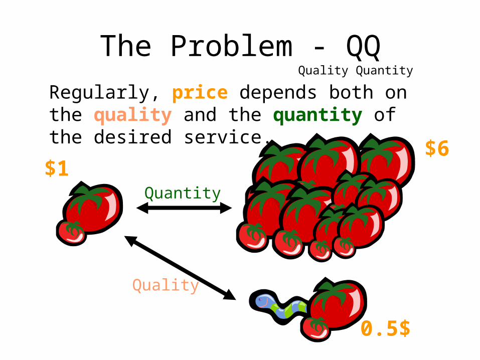
Regularly, price depends both on the quality and the quantity of the desired service.

Quantity

Quality

$1$6

0.5$

The Problem - QQQuality Quantity

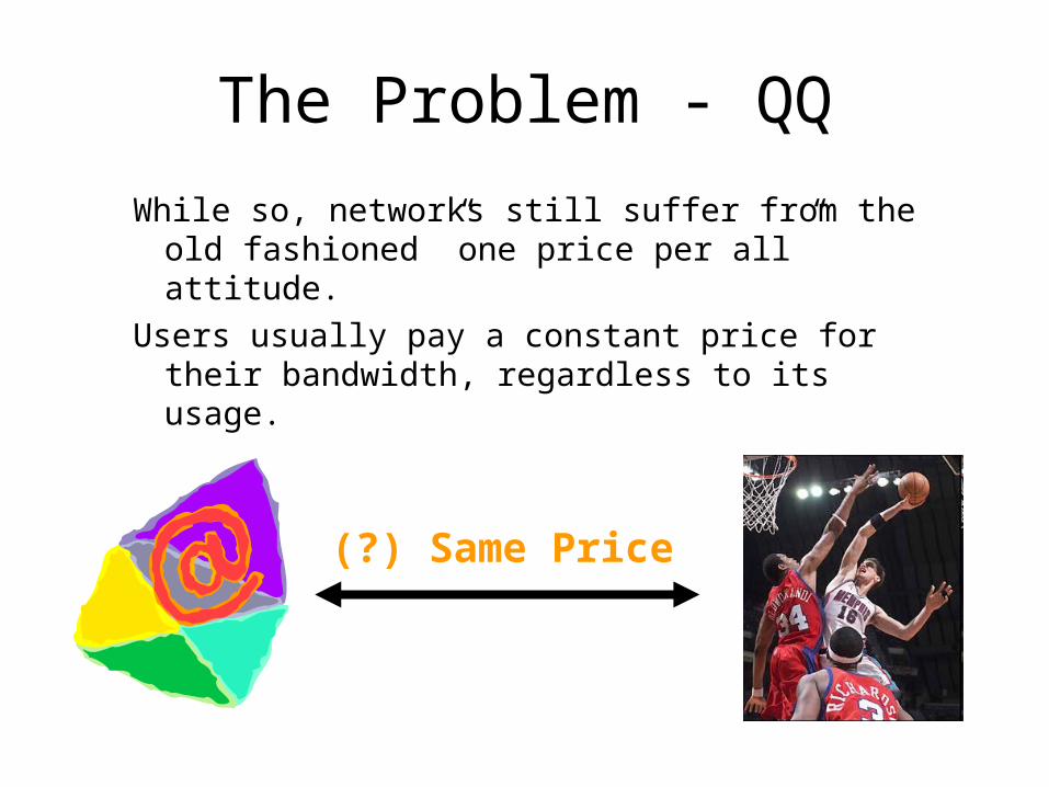
The Problem - QQ

While so, networks still suffer from the old fashioned ”one price per all” attitude.

Users usually pay a constant price for their bandwidth, regardless to its usage.

Same Price)?(

The Problem - QQ

• Many QoS (Quality of Service) protocols have been recently developed in order to solve the problem above.

• We have chosen to use the “Differentiated Services” approach.

Differentiated Services

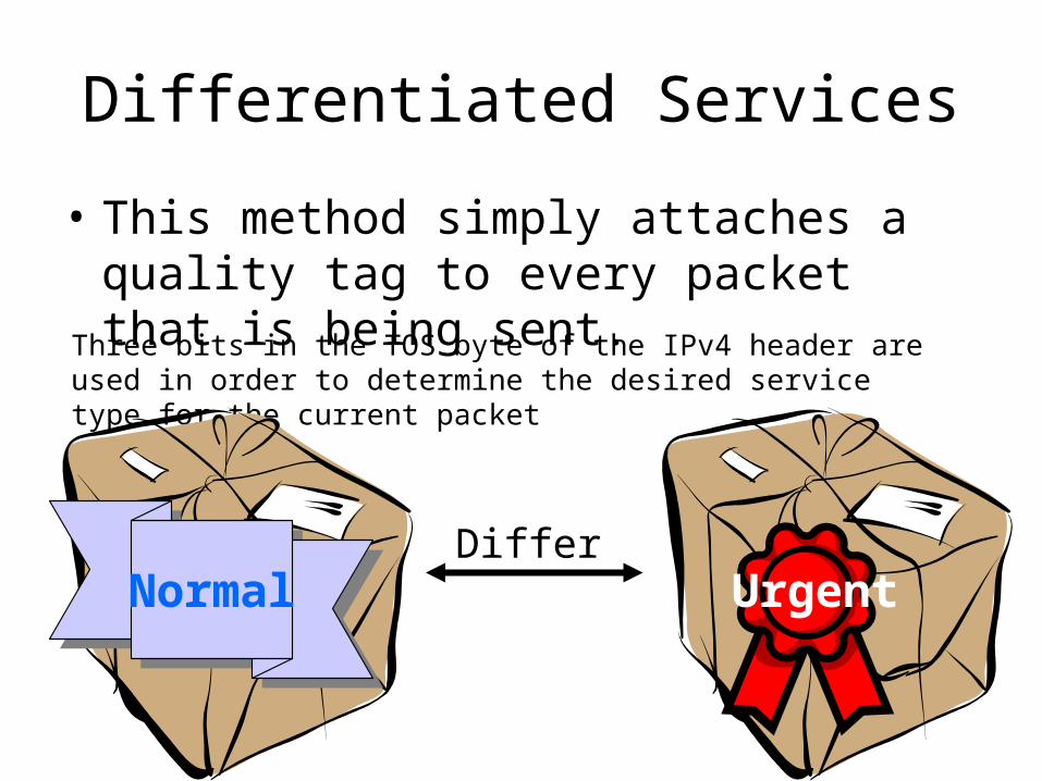
• This method simply attaches a quality tag to every packet that is being sent.

Three bits in the TOS byte of the IPv4 header are used in order to determine the desired service type for the current packet

UrgentDiffer

Normal

The Dynamic Nature

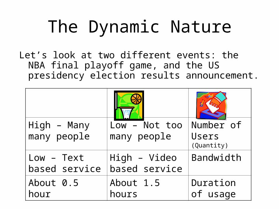
Let’s look at two different events: the NBA final playoff game, and the US presidency election results announcement.

Number of Users (Quantity)

Low – Not too many people

High – Many many people

BandwidthHigh – Video based service

Low – Text based service

Duration of usage

About 1.5 hoursAbout 0.5 hour

The Dynamic Nature

These events were predictable.

What about unpredictable events such as news flashes ?

This kind of events cause a dramatic change in the service requests characteristics.

The Dynamic Nature

Our service supplier should be able to operate under our dynamic world – thus be flexible and rapidly adjustable.

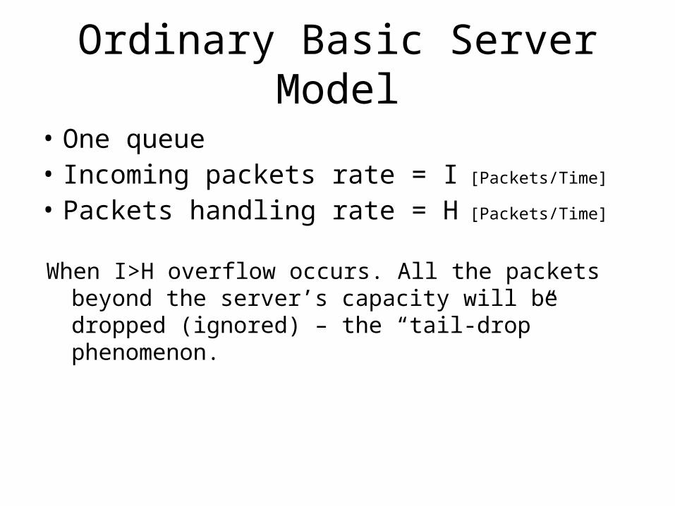
Ordinary Basic Server Model

• One queue• Incoming packets rate = I [Packets/Time]

• Packets handling rate = H [Packets/Time]

When I>H overflow occurs. All the packets beyond the server’s capacity will be dropped (ignored) – the “tail-drop” phenomenon.

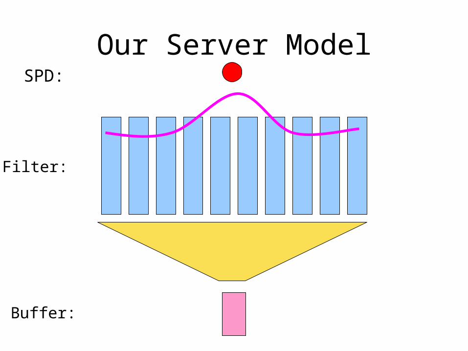
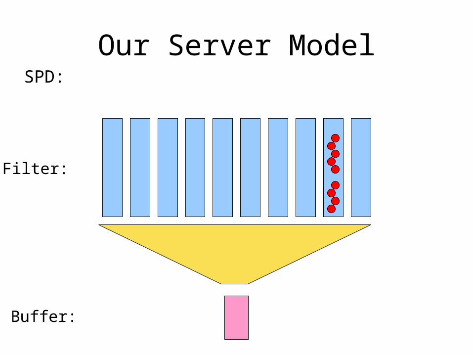
Our Server Model

• Our server will be divided into a filter and a buffer.• The filter will be constructed out of several queues,

each with its own length and packet-loss rate. • We will use 10 queues in our filter. A packet in the 1st

(left most) queue has probability of 0.1 not to be dropped, while a packet in the 10th queue will be handled for sure.

Our Server Model

• Every packet that reaches the server contains some information about where it should be placed (using Differentiated Services). The server is in charge of spreading the packets between the different queues in the filter.

• SPD (Service-based Packet Dropping) is the filtering scheme, used to drop packets according to the queue they are in.

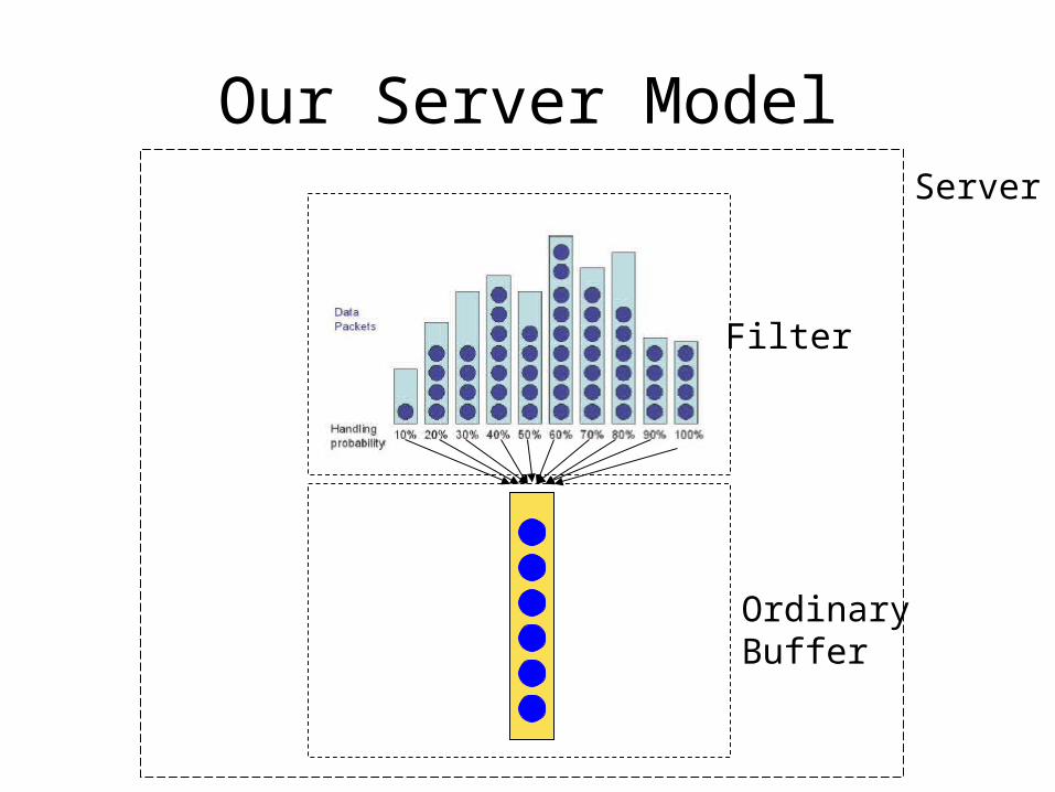
Our Server Model

Filter

OrdinaryBuffer

Server

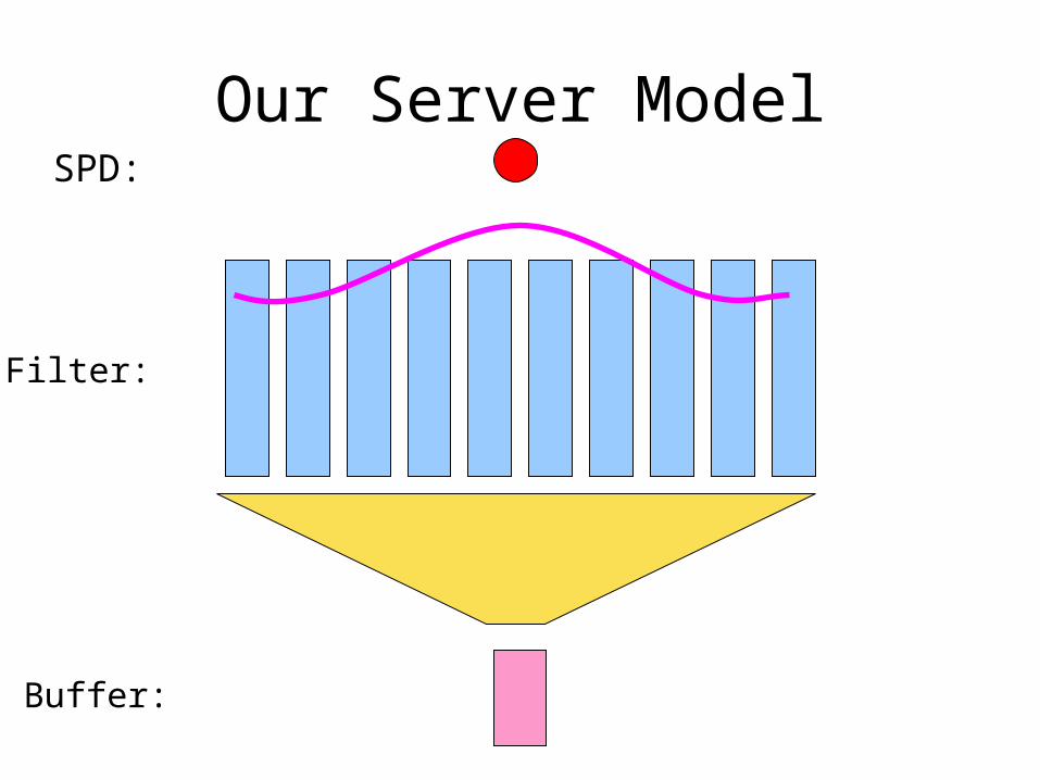
Our Server Model

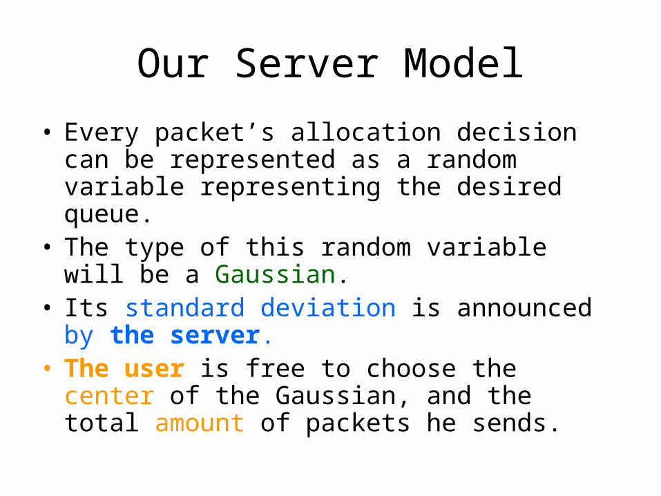
• Every packet’s allocation decision can be represented as a random variable representing the desired queue.

• The type of this random variable will be a Gaussian.

• Its standard deviation is announced by the server.

• The user is free to choose the center of the Gaussian, and the total amount of packets he sends.

A Methodical Break

• Where did this idea come from?

The roots of this project are the physical variables from the world of statistical mechanics.

The work tries to construct the server under certain temperature (1/β) and users with chemical potential (μ).

The users try to achieve equilibrium with their environment (the server), just like any physical system we know.

Some SPD examples

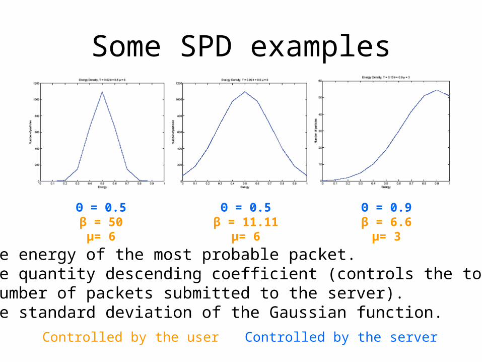
Θ – The energy of the most probable packet. μ – The quantity descending coefficient (controls the total

number of packets submitted to the server).β – The standard deviation of the Gaussian function.

Θ = 0.5β = 50μ= 6

Θ = 0.5β = 11.11

μ= 6

Θ = 0.9β = 6.6

μ= 3

Controlled by the serverControlled by the user

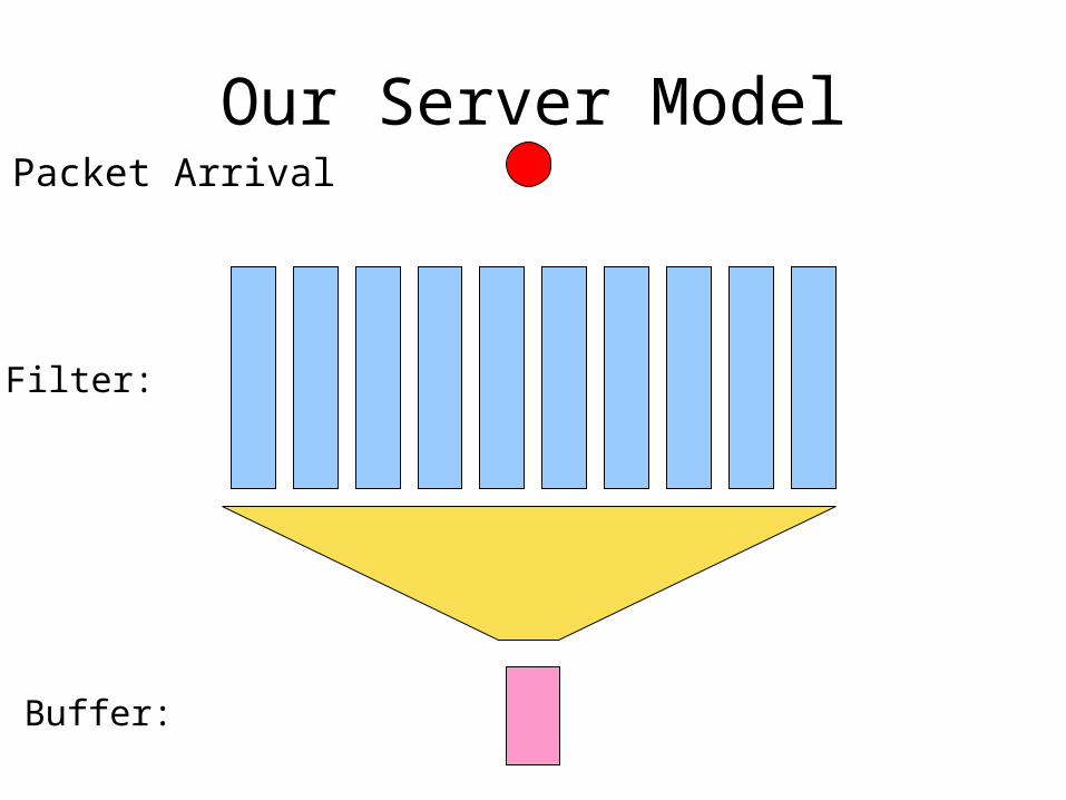
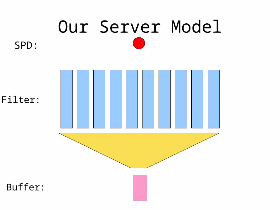
Our Server Model

Filter:

Buffer:

Packet Arrival

Our Server Model

Filter:

Buffer:

SPD:

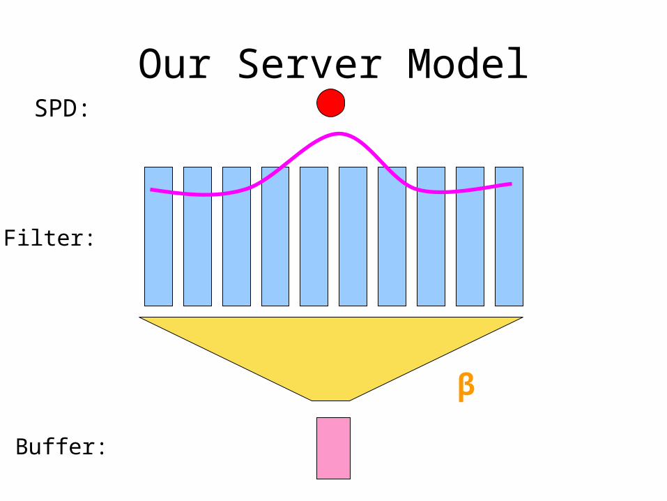
Our Server Model

Filter:

Buffer:

SPD:

β

Our Server Model

Filter:

Buffer:

SPD:

Our Server Model

Filter:

Buffer:

SPD: Θ

Our Server Model

Filter:

Buffer:

SPD:

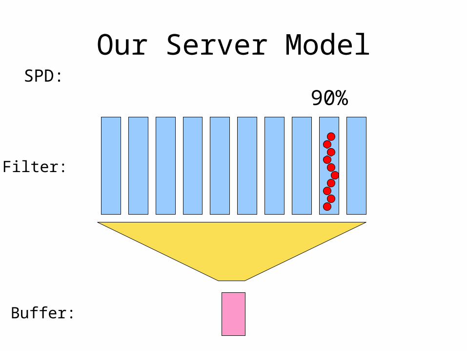
Our Server Model

Filter:

Buffer:

SPD:90%

Our Server Model

Filter:

Buffer:

SPD:

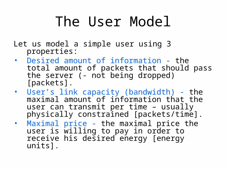
The User Model

Let us model a simple user using 3 properties:• Desired amount of information - the total

amount of packets that should pass the server (- not being dropped) [packets].

• User’s link capacity (bandwidth) - the maximal amount of information that the user can transmit per time – usually physically constrained [packets/time].

• Maximal price - the maximal price the user is willing to pay in order to receive his desired energy [energy units].

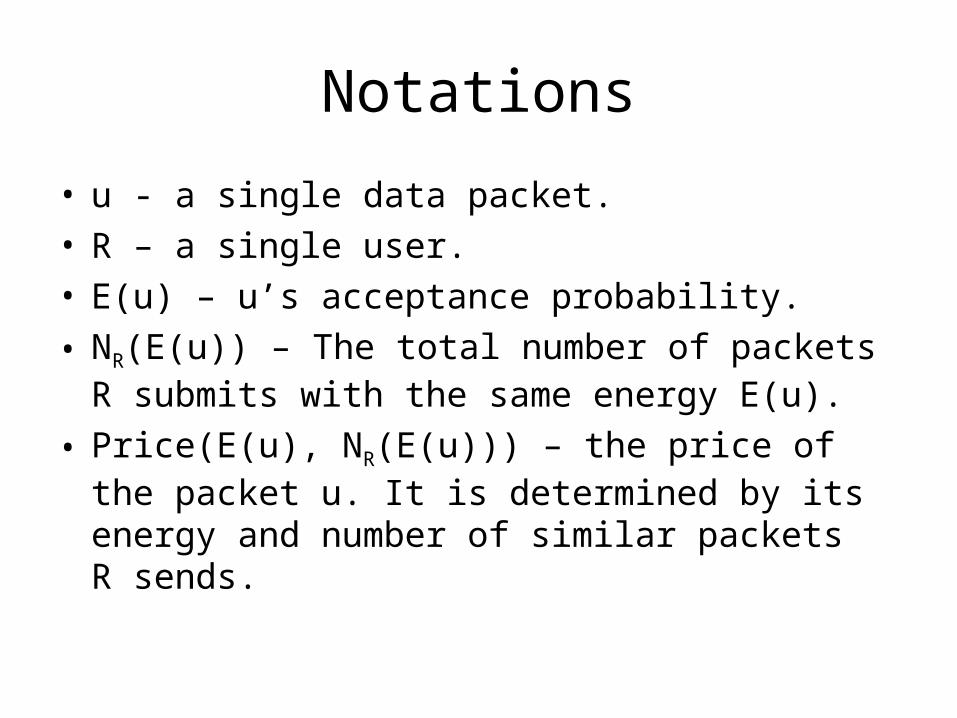
Notations

• u - a single data packet.• R – a single user.• E(u) – u’s acceptance probability.

• NR(E(u)) – The total number of packets R submits with the same energy E(u).

• Price(E(u), NR(E(u))) – the price of the packet u. It is determined by its energy and number of similar packets R sends.

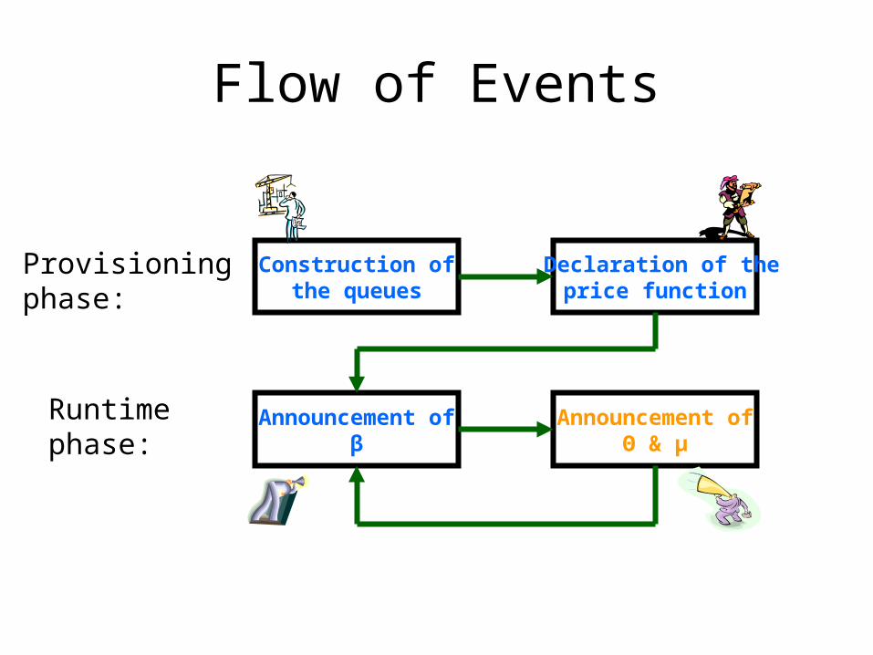
Flow of Events

Declaration of the price function

Construction ofthe queues

Provisioning phase:

Runtime phase:

Announcement ofβ

Announcement ofΘ & μ

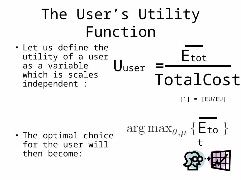
The User’s Utility Function

• Let us define the utility of a user as a variable which is scales independent :

• The optimal choice for the user will then become:

]EU/EU] = [1[

Uuser =Etot

TotalCost

Etot

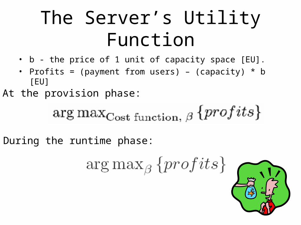
The Server’s Utility Function

• b - the price of 1 unit of capacity space [EU].• Profits = (payment from users) – (capacity) * b [EU]

At the provision phase:

During the runtime phase:

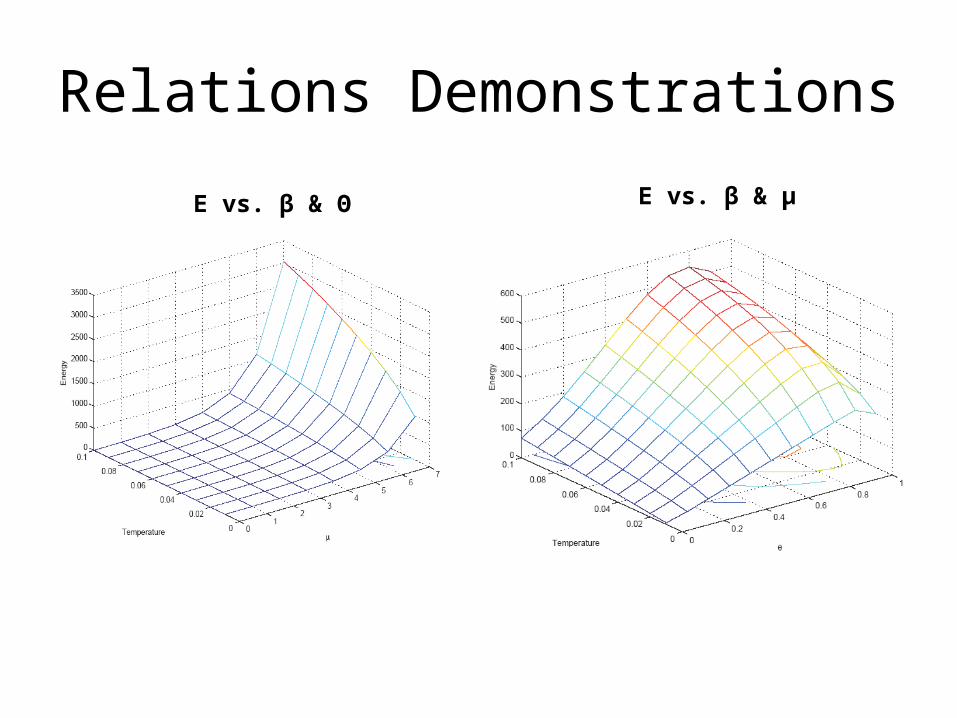
Relations Demonstrations

E vs. β & Θ E vs. β & μ

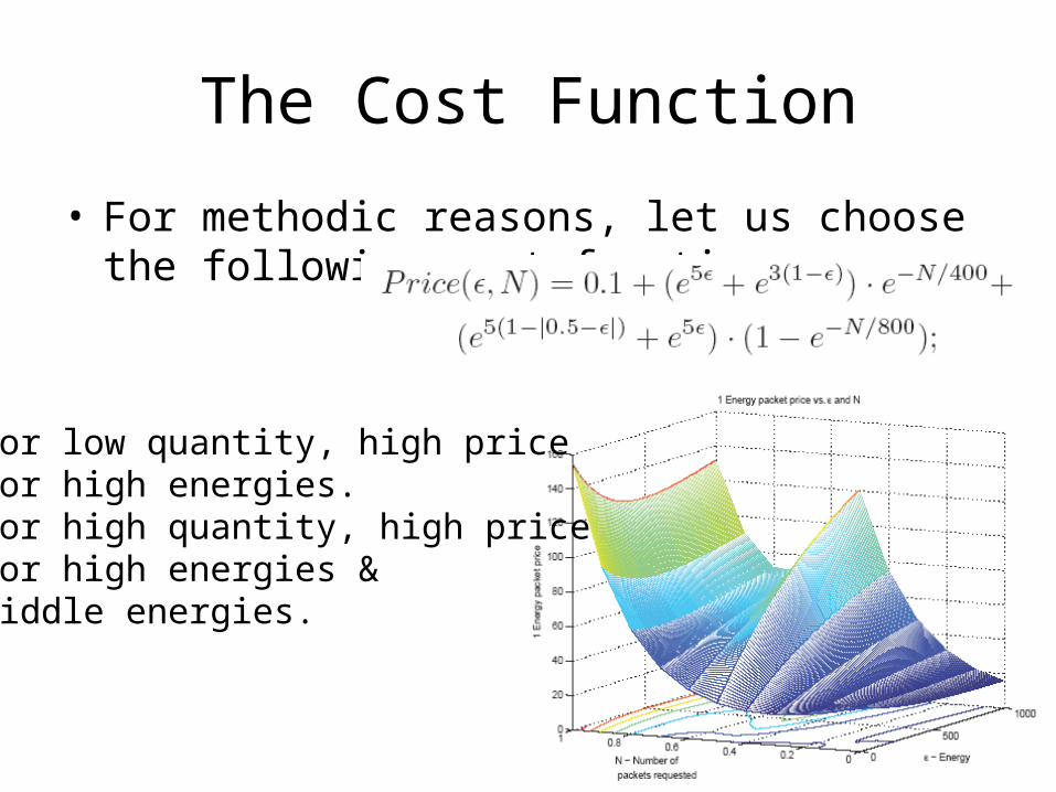
The Cost Function

• For methodic reasons, let us choose the following cost function:

For low quantity, high pricefor high energies. For high quantity, high price for high energies & middle energies.

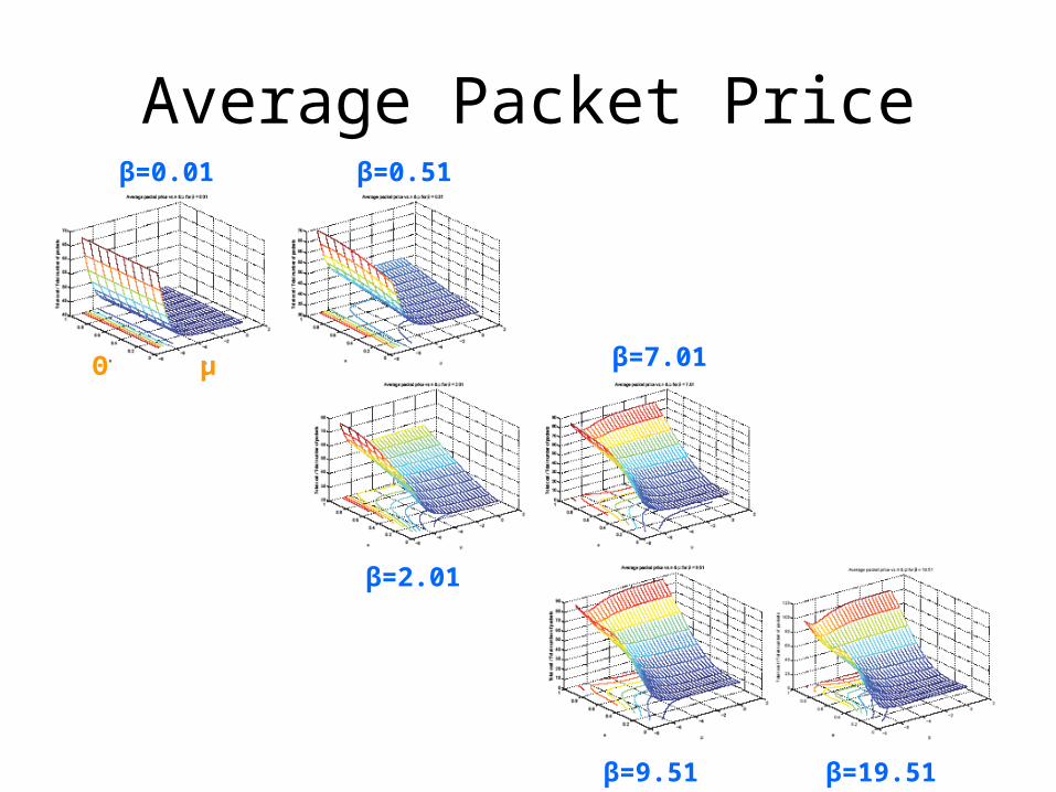
Average Packet Price

Θ μ

β=0.01 β=0.51

β=2.01

β=7.01

β=9.51 β=19.51

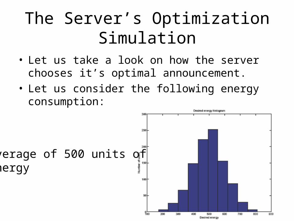
The Server’s Optimization Simulation

• Let us take a look on how the server chooses it’s optimal announcement.

• Let us consider the following energy consumption:

Average of 500 units of energy

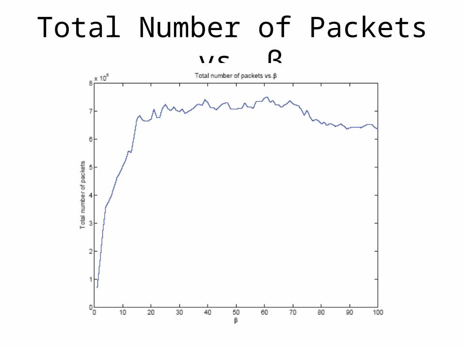
Total Number of Packets vs. β

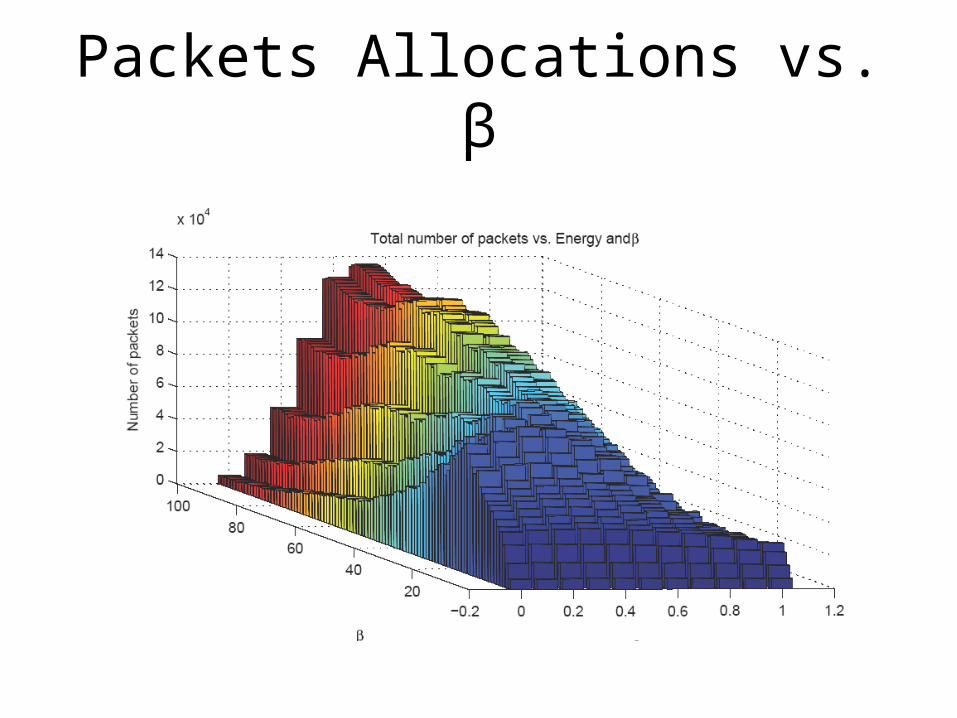
Packets Allocations vs. β

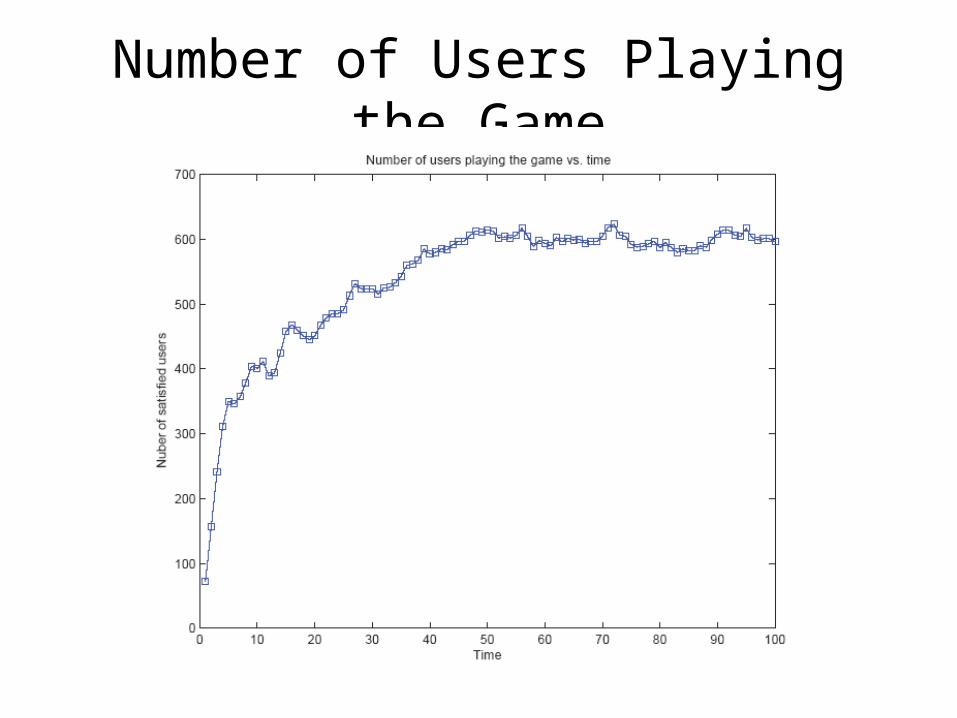
Number of Users Playing the Game

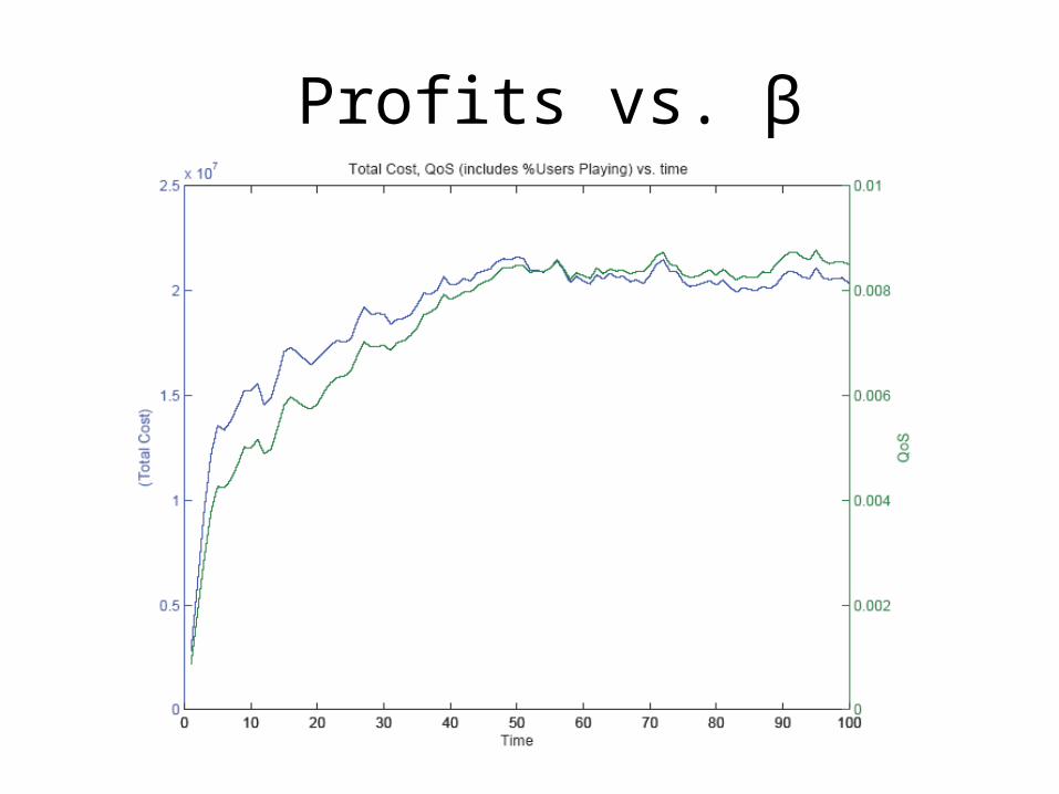
Profits vs. β

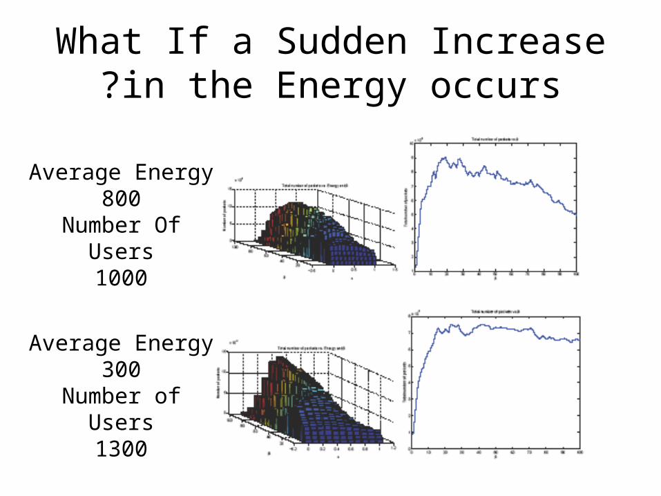
What If a Sudden Increase in the Energy occurs?

Average Energy 800

Number Of Users1000

Average Energy 300

Number of Users1300

What If a Sudden Increase in the Energy occurs?

• Under the right choice of β, the server can handle sudden changes in its demands.

• The right choice here means that the total number of packets the server needs to handle does not vary too much, and thus no physical constraint will affect the server’s operations.

One Day Game

After showing how the server chooses β, let us introduce a simple simulation that will try to estimate the network traffic for "one day”.

Different hours of the day will gain different services desires.

Let us choose the queues of the server to be 10,000 packet places long each.

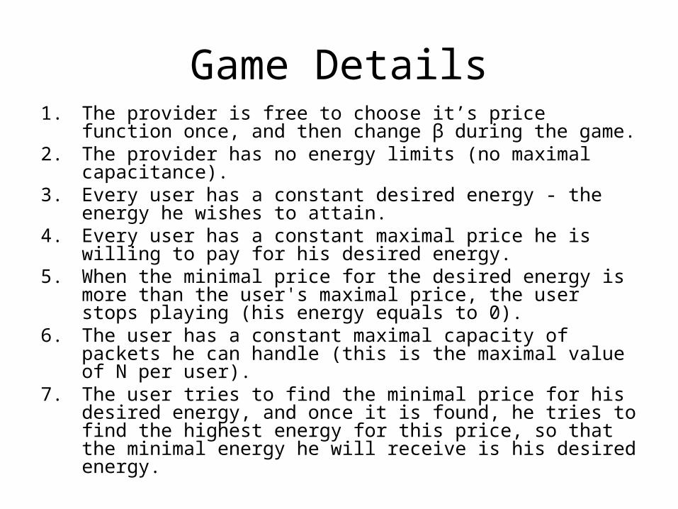
Game Details1. The provider is free to choose it’s price function once, and

then change β during the game.2. The provider has no energy limits (no maximal

capacitance).3. Every user has a constant desired energy - the energy he

wishes to attain.4. Every user has a constant maximal price he is willing to pay

for his desired energy.5. When the minimal price for the desired energy is more than

the user's maximal price, the user stops playing (his energy equals to 0).

6. The user has a constant maximal capacity of packets he can handle (this is the maximal value of N per user).

7. The user tries to find the minimal price for his desired energy, and once it is found, he tries to find the highest energy for this price, so that the minimal energy he will receive is his desired energy.

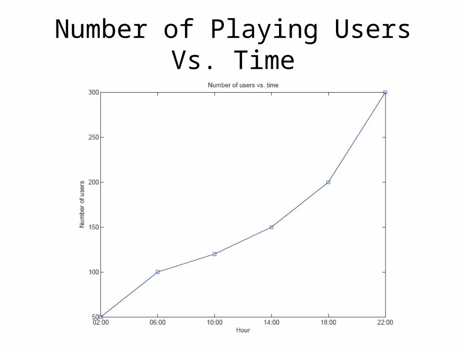
Number of Playing Users Vs. Time

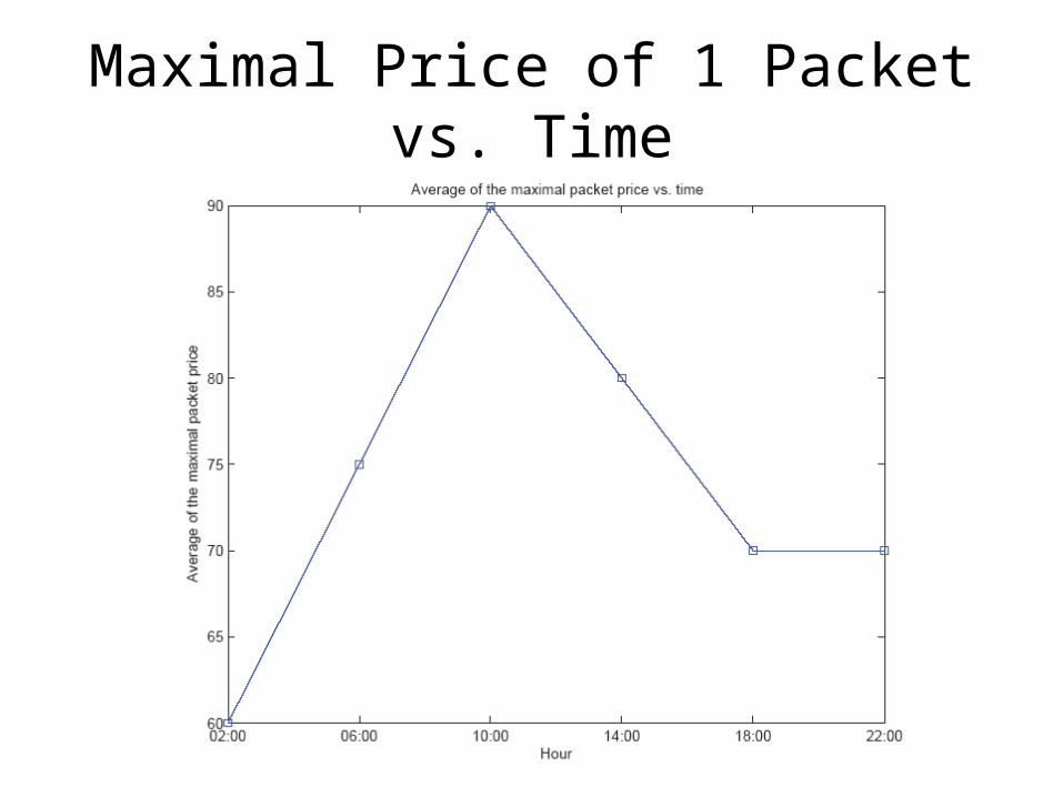
Maximal Price of 1 Packet vs. Time

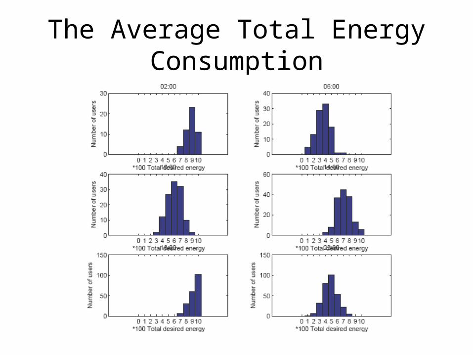
The Average Total Energy Consumption

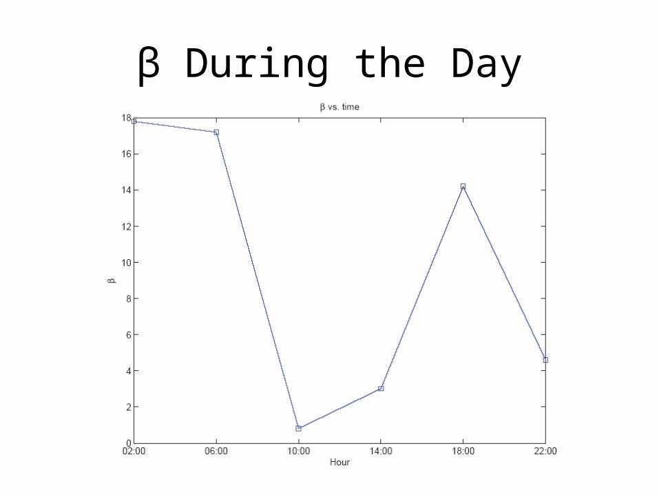
β During the Day

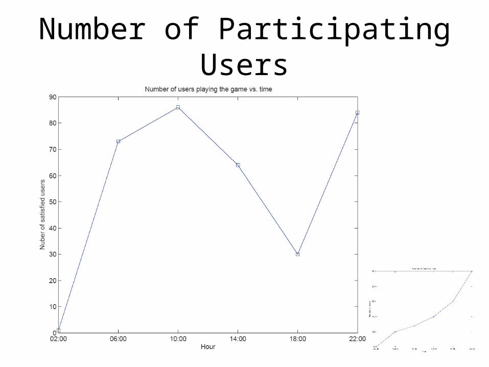
Number of Participating Users

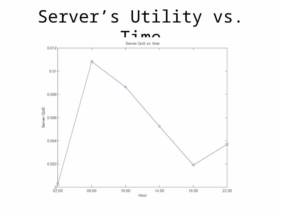
Server’s Utility vs. Time

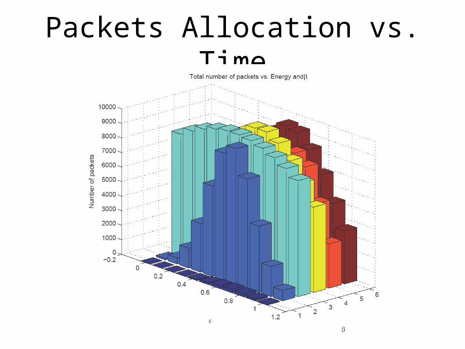
Packets Allocation vs. Time

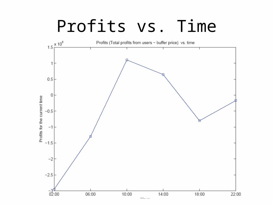
Profits vs. Time

Summary and Conclusions

• In real life, the most general model should allow one user to send multiple requests for services at the same time.

• We observed high correlation between the different variables of the problem. Slight change in the average energy for example, as shown before, can dramatically change the number of users participating the game.

Summary and Conclusions

In spite of the high correlated variables, we were able to answer our server needs:

• Under the right design, a server based on our model can offer multiple services, based upon Quality & Quantity.

• We showed that our server is able to handle sudden changes in the needs of its users.

Finally, The End

• Thank you for listening.