Int. Symp. on Stratified Flows, San Diego, USA, Aug. 29 - Sept. 1, 2016 1

Modeling oxygen depletion within stratified bottom boundary layers of lakes

Aidin Jabbari1, Leon Boegman1, Murray MacKay2, Nader Nakhaei1

1. Environmental Fluid Dynamics Laboratory, Department of Civil Engineering, Queen’s University, Kingston, ON, Canada

0saj@queensu.ca 2. Science and Technology Branch, Environment and Climate Change Canada,

Toronto, ON, Canada Abstract

We have implemented two bottom boundary layer mixing sub-models in a one-dimensional bulk mixed-layer thermodynamic and dissolved oxygen model to diffuse the effects of the sediment oxygen demand from the bottom boundary condition in small lakes. In the first sub-model, bottom mixing is calculated following a mixed layer approach, whereas in the second sub-model the dissolved oxygen flux is computed from Fick’s Law. The second sub-model results in better prediction of dissolved oxygen in two small Canadian Shield lakes, compared to the mixed-layer approach. While appropriate for the upper mixed layer, the bottom mixed-layer model produced excessive near-bed mixing. Bottom mixed layer approaches have been successful in large lakes, suggesting a Reynolds number dependence for mixed-layer development. 1 Introduction

Mixed-layer models are efficient to predict thermal structure in large lakes (e.g., Ivey and Patterson, 1984), when there is strong stratification and a near-isothermal bottom mixed layer (BML) develops during the summer. Interactions between the BML and the overlying flow, which regulates the BML thickness (Valipour et al., 2015), are crucial in controlling the dissolved oxygen (DO) concentration profile through the watercolumn. However, formation of a fully turbulent BML in small lakes is less likely (Boehrer et al., 2008; Fee et al., 1996) and a mixed layer approach might not be appropriate to predict DO profiles close to the bed. In this study, we compare the results from a well-known mixed layer sub-model (Imberger, 1985; Spigel et al., 1986) with those from a Fickian diffusive flux, applied to compute the DO through the watercolumn of two small Canadian Shield Lakes. The oxygen models were calibrated and validated by hind-casting temperature and DO profiles. The validated model will be applied over climate-change relevant timescales, and validated against DO

Int. Symp. on Stratified Flows, San Diego, USA, Aug. 29 - Sept. 1, 2016 2

reconstructions from sediment cores to predict future deep-water temperature and DO concentrations in Canadian Lake Trout lakes as a tool for fishery management.

2 Methods A simple DO sub-model (following Hamilton and Schladow, 1997), has been embedded in the one-dimensional bulk mixed-layer thermodynamic Canadian Small Lake Model (CSLM; MacKay, 2012). This model is currently being incorporated into the Canadian Land Surface Scheme (CLASS), the primary land surface component of Environment and Climate Change Canada’s global and regional climate modeling system. The Mosaic approach (Koster and Suarez, 1992), in which grid cells are divided into lake tiles (1 m2 watercolumns), is used in CSLM to handle complex heterogeneous terrain within a grid cell. Through this approach, hundreds of small lakes can be represented with a few idealized lake tiles.

CSLM has no mixing below the upper mixed layer, and so to diffuse upwards in the watercolumn the effects of the sediment oxygen demand (SOD) from the bottom boundary condition, we have implemented two bottom boundary layer mixing sub-models. In the first

sub-model, bottom mixed layer thickness (ℎ!"#) is calculated following a mixed layer

approach (Imberger, 1985; Spigel et al., 1986) 𝑑(𝑢ℎ!"#) 𝑑𝑡 = 𝑢!∗!, where 𝑢 is the mixed-

layer velocity and 𝑢!∗ is the bottom friction velocity (𝑢!∗ = 0.2𝑢!∗, where 𝑢!∗ is surface friction velocity calculated from near surface wind speed (Ivey and Patterson, 1984). Details of the numerical scheme and parameterizations are provided in MacKay (2012). This approach calculates a fully turbulent BML with a uniform DO that results from stirring, shear and buoyancy production. In the second sub-model, the DO flux is computed from Fick’s Law

𝐽 = −𝐾 𝑑𝐷𝑂 ⁄ 𝑑𝑧. Here, the turbulent diffusivity is considered constant (K=10-7 m2s−1) and is an average from diffusivities measured with a microstructure profiler (Nakhaei et al., 2016). To calibrate and validate the model, we have used two data sets that include 5 years of high-frequency (10 s to 10 min) observations from Eagle Lake (44°40′ N 76°42′ W, maximum depth=30 m, (surface area)1/2 = 250 m) and 30 years of bi-weekly data from Harp Lake (45°38′ N 79°13′ W, maximum depth 34 m, (surface area)1/2 = 843 m). Figure 1 shows the temperature and DO time series from the model with Fickian flux for Harp Lake (July 5th, 1978 to December 31th, 2007) and Eagle Lake (June 22nd, 2011 to July 29th, 2015). Model vertical grid resolution and timestep are 0.5 m and 10 min, respectively, for both lakes.

Below the thermocline, hypolimnetic oxygen demand (HOD; sum of respiration and photosynthesis) and sediment oxygen demand (SOD) play as sinks of DO (Bouffard et al., 2013). Obtained through calibration of the model, HOD is parameterized using constant values of 0.03 gm-3d-1 and 0.08 gm-3d-1 for Harp Lake and Eagle Lake, respectively. SOD is

Int. Symp. on Stratified Flows, San Diego, USA, Aug. 29 - Sept. 1, 2016 3

applied to the first cell above the bed and is calculated using a simple biochemical-based

model (Walker and Snodgrass, 1986) 𝑆𝑂𝐷 = 𝜇! 𝐷𝑂 ⁄ (𝐷𝑂 + 𝐾!)𝛼!"#!!!", where 𝜇!=0.46 gm-

2d-1 is the maximum biochemical sediment oxygen uptake (Bouffard et al., 2013), 𝐾!=1.5 mgL-1 is the half saturation constant for DO (Robson and Hamilton, 2004), 𝛼!"#=1.08 is the sediment temperature multiplier for release rate (Robson and Hamilton, 2004), and T is the temperature in degrees Kelvin.

Figure 1: S i m u l a t e d H a r p L a k e ( a ) temperature (°C) and (b) dissolved Oxygen (mgL-1) and Eagle Lake ( c ) temperature (°C) and (d) dissolved oxygen (mgL-1) profiles.

3 Results Comparison of temperature and DO profiles from the original model with no mixing scheme beyond the upper mixed layer against the observations shows that the model predicts temperature (Figures 2a and 2e) and DO profiles (Figures 2b and 2f) with RMS error (eT and

Int. Symp. on Stratified Flows, San Diego, USA, Aug. 29 - Sept. 1, 2016 4

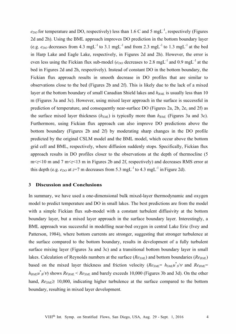
eDO for temperature and DO, respectively) less than 1.6 C and 5 mgL-1, respectively (Figures 2d and 2h). Using the BML approach improves DO prediction in the bottom boundary layer (e.g. eDO decreases from 4.3 mgL-1 to 3.1 mgL-1 and from 2.3 mgL-1 to 1.3 mgL-1 at the bed in Harp Lake and Eagle Lake, respectively, in Figures 2d and 2h). However, the error is even less using the Fickian flux sub-model (eDO decreases to 2.8 mgL-1 and 0.9 mgL-1 at the bed in Figures 2d and 2h, respectively). Instead of constant DO in the bottom boundary, the Fickian flux approach results in smooth decrease in DO profiles that are similar to observations close to the bed (Figures 2b and 2f). This is likely due to the lack of a mixed layer at the bottom boundary of small Canadian Shield lakes and hBML is usually less than 10 m (Figures 3a and 3c). However, using mixed layer approach in the surface is successful in prediction of temperature, and consequently near-surface DO (Figures 2a, 2b, 2e, and 2f) as the surface mixed layer thickness (hSML) is typically more than hBML (Figures 3a and 3c). Furthermore, using Fickian flux approach can also improve DO predictions above the bottom boundary (Figures 2b and 2f) by moderating sharp changes in the DO profile predicted by the original CSLM model and the BML model, which occur above the bottom grid cell and BML, respectively, where diffusion suddenly stops. Specifically, Fickian flux approach results in DO profiles closer to the observations at the depth of thermocline (5 m<z<10 m and 7 m<z<13 m in Figures 2b and 2f, respectively) and decreases RMS error at this depth (e.g. eDO at z=7 m decreases from 5.3 mgL-1 to 4.3 mgL-1 in Figure 2d).

3 Discussion and Conclusions In summary, we have used a one-dimensional bulk mixed-layer thermodynamic and oxygen model to predict temperature and DO in small lakes. The best predictions are from the model with a simple Fickian flux sub-model with a constant turbulent diffusivity at the bottom boundary layer, but a mixed layer approach in the surface boundary layer. Interestingly, a BML approach was successful in modelling near-bed oxygen in central Lake Erie (Ivey and Patterson, 1984), where bottom currents are stronger, suggesting that stronger turbulence at the surface compared to the bottom boundary, results in development of a fully turbulent surface mixing layer (Figures 3a and 3c) and a transitional bottom boundary layer in small lakes. Calculation of Reynolds numbers at the surface (ReSML) and bottom boundaries (ReBML)

based on the mixed layer thickness and friction velocity (ReSML= hSMLu*S/ν and ReBML=

hBMLu*B/ν) shows ReBML < ReSML and barely exceeds 10,000 (Figures 3b and 3d). On the other

hand, ReSML≥ 10,000, indicating higher turbulence at the surface compared to the bottom

boundary, resulting in mixed layer development.

Int. Symp. on Stratified Flows, San Diego, USA, Aug. 29 - Sept. 1, 2016 5

Conversely, in the bottom boundary of Lake Erie, where typically u*B=0.2 cm/s and

hBML≈7 m, (Ivey and Patterson, 1984) ReBML is more than 10,000 and BML approach is

successful. These results suggest a Reynolds number dependence for mixed layer development, where for Reynolds numbers < 10,000 the flow remains transitional and a Fickian diffusion model is appropriate, whereas for Reynolds numbers > 10,000, we expect a fully turbulent boundary layer and a mixed layer model should be used.

Future work will extend these models to investigate relationships between climate and deep-water hypoxia in lake trout lakes. For example, the ReSML approach can be applied to better understand lake turnover and associated re-oxygenation of the hypolimnion in spring and fall. Lakes with small fetch lengths (Molot et al., 1992) and incomplete spring turnover (Boegman et al., 2012) have been shown to not fully mix oxygen to depth, leading to a low hypolimnion oxygen initial condition in spring and consequently more severe summer

hypoxia. This occurs in Eagle Lake (e.g., Figure 1d, spring of 2014), where ReSML≈13,000

(associated with hSML≈3 m) is low compared to ReSML in the previous years (Figure 3d). These

results will be further investigated elsewhere.

Figure 2: Comparison of temperature (°C) (a and e) and dissolved oxygen (mgL-1) (b and f) from observations with various model results and RMS error for temperature (°C) (c and g) and dissolved oxygen (mgL-1) (d and h) for Harp Lake (a, b, c, and d; a and b are for Sep. 15th, 1999) and Eagle Lake (e, f, g, and h; e and f are for Sep. 22nd, 2011). In a, b, e, and f observations are in black. Colors in d and h are consistent with those in b and f; green: model with Fickian flux sub-model, magenta: model using BML approach, and blue: original model without bottom boundary sub-model.

z(m)

0

10

20

30

35

T (C)0 10 20

z(m)

0

10

20

30

observ.

model

DO(mgL−1)

0 5 10

observ.

eT (C)0 1 2

eDO(mgL−1)0 2 4 6

model(Fickianflux)model(BML)model

e

Harp Lake a

Eagle Lake

b

f

c

g

d

h

Int. Symp. on Stratified Flows, San Diego, USA, Aug. 29 - Sept. 1, 2016 6

Figure 3: Surface and bottom mixed layer thicknesses (a and c) and surface and bottom mixed layer Reynolds numbers (b and d) for Harp Lake (a and b) and Eagle Lake (c and d).

References

Boegman, L. Shkvorets, I., and Johnson, F. (2012). Hypoxia and turnover in a small ice covered temperate lake. Proceedings 21st IAHR International Symposium on Ice, Dalian, China, June 11-15, 12 pp.

Boehrer, B. and Schultze, M. (2008). Stratification of lakes. Rev. Geophys., 46, RG2005, doi:10.1029/2006RG000210.

Bouffard, D., Ackerman, J. D., and Boegman, L. (2013). Factors affecting the development and dynamics of hypoxia in a large shallow stratified lake: hourly to seasonal patterns. Water Resour. Res., 49(5), 2380-2394.

Fee, E. J., Hecky, R. E., Kasian, S. E. M., and Cruikshank, D. R. (1996). Effects of lake size, water clarity, and climatic variability on mixing depths in Canadian Shield lakes. Limnol. Oceanogr., 41, doi: 10.4319/lo.1996.41.5.0912.

Hamilton, D. P. and Schladow, S. G. (1997). Prediction of water quality in lakes and reservoirs. Part I—Model description. Ecol. Model., 96(1), 91-110.

Imberger, J. (1985). The diurnal mixed layer1. Limnol. Oceanogr., 30(4), 737-770. Ivey, G. N. and Patterson, J. C. (1984). A model of the vertical mixing in Lake Erie in

summer. Limnol. Oceanogr., 29(3), 553-563. Koster, R. D. and Suarez, M. J. (1992). Modeling the land surface boundary in climate

models as a composite of independent vegetation stands. J. Geophys. Res., 97 (D3), 2697–2715.

0

10

20

30hSM

L,h

BM

L(m

)

1980 1985 1990 1995 2000 20050

1

2

3

4

5

Re S

ML,R

e BM

L

×104

0

10

20

30

hSM

L,h

BM

L(m

)

2012 2013 2014 2015year

0

5

10

Re S

ML,R

e BM

L

×104

ReSML

ReBML

hSML

hBML

a

b

c

d

Int. Symp. on Stratified Flows, San Diego, USA, Aug. 29 - Sept. 1, 2016 7

MacKay, M. D. (2012). A process-oriented small lake scheme for coupled climate modeling applications. J. Hydrometeorol., 13(6), 1911-1924.

Molot, L.A., Dillon, P.J., Clark, B., and Neary, B (1992). Predicting end-of-summer oxygen profiles in stratified lakes. Canadian Journal of Fisheries and Aquatic Science, 49, 2363-2372.

Nakhaei, N, Boegman, L., and Bouffard, D. (2016). Measurement of vertical oxygen flux in lakes from microstructure casts. Proceedings 8th Int. Symp. on Stratified Flows, San Diego, USA, August 29 – September 1, 2016.

Robson, B. J. and Hamilton, D. P. (2004). Three-dimensional modelling of a Microcystis bloom event in the Swan River estuary, Western Australia. Ecol. Model., 174(1), 203-222.

Spigel, R. H., Imberger, J., and Rayner, K. N. (1986). Modeling the diurnal mixed layer. Limnol. Oceanogr., 31(3), 533-556.

Valipour, R., Bouffard, D., and Boegman, L. (2015). Parameterization of bottom mixed layer and logarithmic layer heights in central Lake Erie. J. Great Lakes Res., 41: 707-718.

Walker, R.R. and Snodgrass, W.J. (1986). Model for sediment oxygen demand in lakes. J. Environ. Engineer., 112(1):25-43.